Embed Size (px)
Citation preview

MANUFACTURED GOODS CONSUMPTION, RELATIVE PRICES AND PRODUCTIVITY
Inclusive and Sustainable Industrial Development Working Paper SeriesWP 6 | 2018

DEPARTMENT OF POLICY, RESEARCH AND STATISTICS
WORKING PAPER 06/2018
Manufactured goods consumption, relative prices and
productivity
Margarida Duarte University of Toronto
UNITED NATIONS INDUSTRIAL DEVELOPMENT ORGANIZATION
Vienna, 2018
This is a background paper for UNIDO Industrial Development Report 2018: Demand for
Manufacturing: Driving Inclusive and Sustainable Industrial Development
The designations employed, descriptions and classifications of countries, and the presentation of the
material in this report do not imply the expression of any opinion whatsoever on the part of the Secretariat
of the United Nations Industrial Development Organization (UNIDO) concerning the legal status of any
country, territory, city or area or of its authorities, or concerning the delimitation of its frontiers or
boundaries, or its economic system or degree of development. The views expressed in this paper do not
necessarily reflect the views of the Secretariat of the UNIDO. The responsibility for opinions expressed
rests solely with the authors, and publication does not constitute an endorsement by UNIDO. Although
great care has been taken to maintain the accuracy of information herein, neither UNIDO nor its member
States assume any responsibility for consequences which may arise from the use of the material. Terms
such as “developed”, “industrialized” and “developing” are intended for statistical convenience and do
not necessarily express a judgment. Any indication of, or reference to, a country, institution or other legal
entity does not constitute an endorsement. Information contained herein may be freely quoted or reprinted
but acknowledgement is requested. This report has been produced without formal United Nations editing.
iii
Table of Contents
1 Introduction ........................................................................................................................... 2
2 Changes in consumption patterns with income ........................................................................ 5
3 Data: sources and analysis ...................................................................................................... 7
4 Results ................................................................................................................................... 9
4.1 Consumption of manufactured goods and services ......................................................... 9
4.2 Individual manufactured goods consumption categories .............................................. 11
4.4 Purpose of use and manufactured consumption ............................................................ 14
4.5 Decomposition by industrial classification ................................................................. 14
5 Mapping to productivity ...................................................................................................... 16
6 Conclusion ........................................................................................................................... 21
References ................................................................................................................................... 22
Appendix A. Manufactured consumption categories .................................................................. 24
Appendix B. Relative prices and expenditure shares by deciles ................................................. 26
List of Tables
Table 1 Manufactured goods by purpose of use ....................................................................... 15
Table 2 Industrial classification – relative prices and expenditure shares ................................... 18
Table 3 Development accounting results ................................................................................... 19
Table 4 Manufactured goods and services ................................................................................. 26
Table 5 Food and non-food manufactured goods ...................................................................... 27
Table 6 Durability .................................................................................................................... 28
Table 7 Manufactured goods and services - ICP2005 ................................................................ 29
Table 8 Food and non-food manufactured goods - ICP2005 ...................................................... 30
List of Figures
Figure 1 Consumption of manufactured goods .......................................................... 31
Figure 2 Consumption of services .............................................................................. 32
Figure 3 Consumption of manufactured goods - food ................................................ 33
Figure 4 Consumption of manufactured goods - non-food ........................................ 34
Figure 5 Audiovisual, photographic, and information processing equipment............ 35
Figure 6 Non-food manufactured goods with declining relative price ....................... 36
Figure 7 Durable goods .............................................................................................. 37
Figure 8 Semi-durable goods ...................................................................................... 38
Figure 9 Non-durable goods ....................................................................................... 39
1
Abstract
The patterns of consumption expenditure in manufactured goods across a broad set of countries
that differ in terms of their level of development are studied, using disaggregated expenditure
and price data from the International Comparisons Program. Across broad categories, the share
of consumption expenditure in manufactured goods consumption falls as income per capita rises
and the share of consumption expenditure increases for services. Among the disaggregated
manufactured goods consumption categories, the patterns are quite varied with the relative price
falling for about 60 per cent of the non-food manufactured goods categories and increasing with
income for the remaining categories. The share of expenditure in non-food manufacturing
categories with a falling relative price increases systematically with income, suggesting a high
degree of substitutability across non-food manufactured goods consumption categories with
different degrees of productivity growth. Expenditure and relative price patterns in
manufactured goods consumption across countries are determined by grouping individual
consumption categories of manufactured goods according to different criteria and productivity
implications associated with the decomposition of manufactured goods consumption by
industrial classification are presented. Differences in productivity are evident across countries
for these manufacturing sub-sectors, but are smaller than those between manufacturing and
services. This result largely reflects the fact that the evolution of relative prices with income is
relatively homogeneous for these sub-sectors.
JEL classification: O1, O4, E0.
Keywords: manufacturing, productivity, relative prices
2
1 Introduction
One of the key stylized facts of economic development is the change in economic structure as
economies grow. Kuznets (1973) identified differences in the share of employment across broad
sectors of agriculture, industry and services as one of the key development factors of modern
economic growth. Using more recent and historical data for a large set of countries and long
time periods, Herrendorf et al. (2014) presented the systematic pattern observed across countries
and over time whereby the share of employment in agriculture falls systematically with income
and the share of employment in services increases systematically with income, while the share
of employment in industry assumes a hump-shape pattern with income (it first rises with income
and then falls). The pattern of consumption across different expenditure categories is associated
with structural transformation; for instance, the decreasing importance of agriculture as income
rises is reflected in a fall in the share of consumption expenditure in food categories. Similarly,
the rise in services with income is reflected in an increase in the share of expenditure in services
as countries develop.
In this paper, patterns in the consumption of manufactured goods and its components across a broad
set of countries that differ in terms of level of development are examined. This focus on patterns of
consumption of manufactured goods follows a growing interest in understanding industrialization
patterns across countries.1 Detailed data on individual consumption expenditure by households
from the International Comparisons Programs (ICP) are used to construct measures of
consumption expenditure measured in domestic prices (nominal expenditure), measures of
consumption expenditure in international prices common across all countries (real expenditure),
and relative prices for different consumption aggregates for a large number of countries at a given
point in time.2 Consumption expenditure and relative prices for two broad consumption
categories—manufactured goods and services—and then decompose manufactured goods
consumption further into food and non-food. The share of consumption expenditure in
manufactured goods declines systematically with development whereas the share of services rises
with income. The price of manufactured goods relative to the price of overall consumption falls with
income, whereas the relative price of services rises with income. That is, relative to the price of
overall consumption, manufactured goods tend to be cheaper in wealthier countries than in
1 See, for instance, Rodrick (2015). 2 In the cross-country comparison literature, the distinction between nominal and real variables refers to whether
prices are country-specific (domestic) or common across countries (international) instead of the traditional distinction
between current and constant prices used in time series analyses.
3
poorer ones, and services tend to be more expensive3. Measuring consumption expenditure
across countries using a common set of international prices (and thus devoid of price differences
across countries), we find that real shares of consumption of manufactured goods also decline
systematically with income but less so than nominal shares. That is, after controlling for price
differences across countries, we find less significant differences across income levels in the share
of consumption expenditure allocated to manufactured goods versus services than the
differences implied by nominal data. The share of non-food categories of manufactured goods
(both nominal and real) in manufactured goods consumption rises systematically with income in
sharp contrast to the development of share of expenditure in food.
Expenditure and relative price patterns in manufactured goods consumption across countries are
examined by grouping individual consumption categories of manufactured goods according to
different criteria. The analysis suggests that most categories of non-food manufactured goods
consumption have a price relative to that of consumption that declines with income. In addition, this
group of non-food categories with a declining relative price also registers expenditure shares
(nominal and real) in total non-food manufactured goods consumption that increase systematically
with income while the group of non-food categories with a rising relative price registers declining
expenditure shares. The observations for these two groups based on the development of relative
prices suggest a high degree of substitutability among non-food manufacturing categories with
different degrees of productivity growth (and relative price developments). We also find that
most aggregations of non-food consumption categories show rising nominal and real expenditure
shares with income, for instance, durable consumption goods or the group of categories associated
with the production of machines.
The productivity implications associated with the decomposition of manufactured goods
consumption by industrial classification are then explored. Using a standard accounting
framework with a minimal structure as in Herrendorf and Valentinyi (2012) and Duarte and
Restuccia (2016), productivity implications are derived using real and nominal expenditure (and
hence, relative price) data for the cross-section of countries. We find some differences in
productivity across countries for these manufacturing sub-sectors, but they are less significant than
those between manufacturing and services. This result largely reflects the fact that the development
3 When making conducting cross-country comparisons, the standard practice is to compare relative prices since prices
are expressed in country-specific currency units. A currency exchange rate can be used to convert prices into a
common currency but, as noted by Summers and Heston (1991), the exchange rate is often a distorted price in the
economy, and thus PPP comparisons are preferable.
4
of relative price with income is relatively homogeneous for these sub-sectors.4 Finally, focusing
exclusively on non-food manufactured goods consumption categories, we find that productivity
gaps across countries are slightly more pronounced for manufacturing categories that are broadly
associated with the production of chemicals, minerals and metal products.
These results suggest that the scope (in terms of aggregate productivity implications) of
pursuing disaggregated industrial-level policies in the manufacturing sector is not particularly
large. Perhaps one exception is the group of manufacturing industries associated with the
transformation of agricultural products, which reveals the largest productivity gap across income
levels. However, this gap most likely reflects the low productivity level of poor countries in the
agricultural sector rather than the manufacturing production of food. Overall, aggregate industrial-
level policies or institutional reforms may be more successful in closing the productivity gap in this
sector across countries.
This paper relates to the literature on structural transformation including Baumol (1967),
Echevarria (1997), Kongsamut et al. (2001), Ngai and Pissarides (2007) and Duarte and
Restuccia (2010).5 It is also closely related to the literature on expenditure patterns based on
data, which includes Herrendorf and Valentinyi (2012) and Duarte and Restuccia (2016), who
use cross-country data, and Atkeson and Ogaki (1996), who use micro data from India across
households and over time.
The paper is organized as follows. Section 2 analyses the fundamental drivers of manufactured goods
consumption. Section 3 describes the data used in this study and Section 4 presents the results.
Section 5 explores the connection between the results in Section 4 and productivity. Section 6
concludes.
4 This result is largely robust to alternative criteria for the aggregation of individual manufactured goods consumption
categories that do not rely on the development of relative price itself. 5 See also a comprehensive survey in Herrendorf et al. (2014).
5
2 Changes in consumption patterns with income
The starting point for analysing the sectoral composition of the economy is a standard multi-
sector extension of the one sector growth model. This model is driven by growth in productivity
at the sector level.
Suppose that an infinitely-lived household has preferences over consumption sequences of
different types of goods, in particular, agricultural goods (a), manufactured goods (m), and
services (s), and that these preferences are described by utility function U (Ca,t, Cm,t, Cs,t).
Households are endowed with one unit of working time which they can supply to any sector. The
household’s objective is to maximize its utility by choosing sectoral consumption patterns that
satisfy the constraint that total expenditure equals total labour income.
Let us also assume that the production side of the economy is described by linear production
functions in labour in each sector, Yi = AiLi, for i = {a, m, s}. Here, Li is the sectoral labour
input and Ai represents the sectoral productivity of labour. This model entails very simple
mapping from production to consumption and market clearing in each sector hence simply
requires that Yi = Ci, ∀i ∈ {a, m, s}.
In competitive labour and goods markets, profit maximization implies that the price of each
good is inversely related to labour productivity in the sector, pi = w/Ai, where w is the wage
rate. Note that in this model, relative price movements are driven solely by relative changes in
the corresponding sectoral labour productivities.
The literature on structural transformation typically specifies a utility function U (Ca,t, Cm,t, Cs,t)
that allows for two mechanisms supporting reallocation across sectors: 1) income effects, and 2)
relative price (substitution) effects. The income effects follow from a non-homothetic demand
structure for different consumption goods. Such a demand structure implies that reallocation
across sectors (measured as either changes in employment shares or in sectoral shares of nominal
expenditure in total expenditure) occurs in response to changes in income, even when relative
prices remain constant.6 In the context of this model, this occurs when all Ai’s are growing at
the same rate: relative prices are constant, but income is growing. The literature emphasizes
the role of income effects in understanding resource allocation in both agriculture and services.
For example, a utility function that entails a minimum consumption level of agricultural goods can
6 See Kongsamut, Rebelo , and Xie (2001).
6
capture the observation that when income is low, expenditure in these goods represents a large share
of total consumption expenditure, and as income grows the share of expenditure falls.
The relative price effects follow from differential sectoral growth rates of productivity. The
literature has explored the conditions under which preferences (even in the absence of non-
homotheticities) are associated with changes in employment shares or in sectoral shares of nominal
expenditure in total expenditure in response to differential sectoral growth rates of productivity.7
For example, when the growth rate of labour productivity in manufacturing is higher than in
services (as observed in the data), a constant elasticity of the substitution utility function with
a low degree of substitutability between manufacturing and services implies that labour
reallocates from the manufacturing to the service sector as labour becomes relatively less
productive in services relative to manufacturing.
Models of sectoral reallocation that have been used in the literature have arrived at the broad
conclusion that both income and relative price effects are needed to account for the observed process
of structural transformation across agriculture, manufacturing and services. That is, both
mechanisms are needed to account for the reallocation of, say, labour from agriculture to
manufacturing and services in early stages of development and the reallocation of labour from
agriculture and manufacturing to services for higher levels of income. Herrendorg et al. (2013),
for instance, assess the empirical importance of these two effects using both fixed expenditure data
and value added data and emphasize the input-output structure of the economy in this
quantitative assessment. More recently, Comin et al. (2015) have argued that income effects play
a major role in generating structural change using a multi-sector model of structural
transformation with non-homothetic constant-elasticity-of-substitution preferences. In what
follows, patterns of consumption of different types of manufactured goods are identified at a
point in time across countries with different levels of income. Conceptually, these patterns can
either be driven by income effects, relative price effects or both. To be able to provide a
quantitative assessment of the role of each effect in accounting for the data requires the structure
of a model.
7 See Baumol (1967) and Ngai and Pissarides (2007).
7
3 Data: sources and analysis
In this paper, cross-country patterns of manufactured goods consumption are analysed using
International Comparisons Program (ICP) data. The ICP is a global statistical initiative that
collects national prices of a well-defined basket of goods and services for the majority of countries in
the world. Data collected in 2011 comprise price and nominal expenditure data for 155
expenditure categories that add up to gross domestic product (GDP) for 177 countries. These
detailed data are aggregated into higher levels of aggregation (such as GDP) which are
comparable across countries using the Geary-Khamis (GK) approach. This approach has the
desirable property of maintaining additivity. This feature is essential in this analysis since it allows
aggregating any number of categories and computing the share of real expenditure this aggregate in
the real expenditure of a higher aggregate (such as real GDP).
The ICP dataset provides parity and nominal expenditure data for each category (basic
heading) and each country in 2011. The parity 𝑝𝑝𝑖𝑗 for each basic heading i, i = 1, ..., m in
country j, j = 1, ..., n is expressed in units of currency of country j to the numeraire currency
(USD) and the nominal expenditure data, 𝐸𝑖𝑗, is denominated in units of the currency of country
j. Note that adding expenditure in local currency over all categories yields a nominal GDP for each
country, that is, 𝐺𝐷𝑃𝑗 = ∑ 𝐸𝑖𝑗𝑚𝑖=1 . Let’s now define a notional quantity 𝑞𝑖𝑗 of goods/services i
in country j as 𝑞𝑖𝑗 = 𝐸𝑖𝑗 𝑝𝑝𝑖𝑗⁄ . Note that, unlike 𝐸𝑖𝑗, these notional quantities are measured at
a common set of prices (USD) and are, therefore, comparable across countries. The GK procedure
generates international prices πi for each basic heading and a purchasing power parity (PPP) of
GDP, PPPj , for each country that solve the system:
𝑃𝑃𝑃𝑗 =∑ 𝑝𝑝𝑖𝑗𝑚𝑖=1 𝑞𝑖𝑗∑ 𝜋𝑖𝑗𝑚𝑖=1 𝑞𝑖𝑗
𝜋𝑖 =∑𝑝𝑝𝑖𝑗
𝑃𝑃𝑃𝑗
𝑛
𝑗=1
(𝑞𝑖𝑗
∑ 𝑞𝑖𝑗𝑛𝑖=1
)
The first set of equations defines the PPP of GDP for each country, PPPj , as the ratio of
GDP in domestic prices (notional quantities times domestic prices) to GDP in international prices
(notional quantities times international prices). These PPP’s are measured in local currency j
per international dollar. The second set of equations defines the international price for each
category i as a weighted average of prices for that category across countries. The weight of each
country is its share of notional quantities in category i. Intuitively, the international prices are
defined so that they imply a purchasing power parity over GDP for each country that is
8
consistent with these prices. After computing international prices, the dataset is restricted to
countries with more than 1 million inhabitants, resulting in 142 countries in the dataset.
After computing international prices, any set of categories can be defined and total
expenditure in local prices, total expenditure in international prices and PPP for each country in the
dataset computed. For example, suppose that the set C includes all individual categories i in
personal consumption expenditure. Then, for each country j,
consumption expenditures in local prices (nominal expenditures) is given by 𝐸𝐶𝑗 =
∑ 𝐸𝑖𝑗𝑖∈𝐶 = ∑ 𝑝𝑝𝑖𝑗𝑞𝑖𝑗𝑖∈𝐶 ;
share of consumption expenditures in GDP in local prices (nominal share) is given by
𝑠𝐸𝑖𝑗 = ∑ 𝐸𝑖𝑗𝑖∈𝐶 ∑ 𝐸𝑖𝑗𝑚𝑖⁄ ;
consumption expenditures in international prices (real expenditures) is given by 𝑄𝐶𝑗 =
∑ 𝜋𝑖𝑞𝑖𝑗𝑖∈𝐶 ;
share of consumption expenditures in GDP in international prices (real share) is given
by
𝑠𝑄𝐶𝑗 = ∑ 𝜋𝑖𝑞𝑖𝑗𝑖∈𝐶 ∑ 𝜋𝑖𝑞𝑖𝑗𝑚𝑖⁄ ;
price of consumption relative to the price of GDP" is given by 𝑅𝑃𝐶𝑗 = 𝑃𝑃𝑃𝐶𝑗 𝑃𝑃𝑃𝑗⁄
where 𝑃𝑃𝑃𝐶𝑗 = 𝐸𝐶𝑗 𝑄𝑗⁄ and the PPP of GDP, 𝑃𝑃𝑃𝑗 is defined above.
Note that in the context of ICP data, nominal variables refer to variables in local prices and real
variables (also often referred to as “PPP-adjusted”) and to variables in international prices. Note
that the meaning of the term “real” in the context of cross-section ICP data is analogous to its
meaning in the context of time-series data. In the context of time-series data, a nominal variable Yt
is measured in year-t money units (say, dollars) while a real variable is measured in dollars in a
base year. This change of units allows for the comparison of quantities over time by removing the
price effect across time. In the context of cross-section ICP data, a nominal variable Yj is
measured in country-j prices while a real variable is measured in international prices (common
across countries). This change of units, by removing the price effect across countries, allows the
use of real variables for the comparison of “quantities” across countries.
9
4 Results
In this section, the development of the consumption of manufactured goods and their components
across the sample of countries in the ICP data is documented. The ICP breaks down individual
consumption expenditure by households into categories by following the Classification of
Individual Consumption According to Purpose (COICOP). We focus on the development of both
nominal and real shares, as well as relative prices.
4.1 Consumption of manufactured goods and services
We first decompose consumption expenditure into two broad categories: manufactured goods and
services. The COICOP is attributed to each consumption expenditure category and services are
mapped to all the service categories in COICOP and manufactured goods to the goods
categories (comprising “Durable goods” plus “Semi-durable goods” plus “Non-durable goods”).8
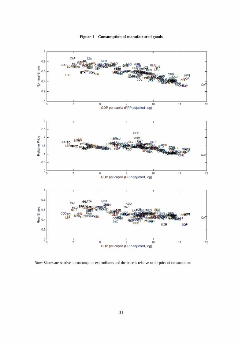
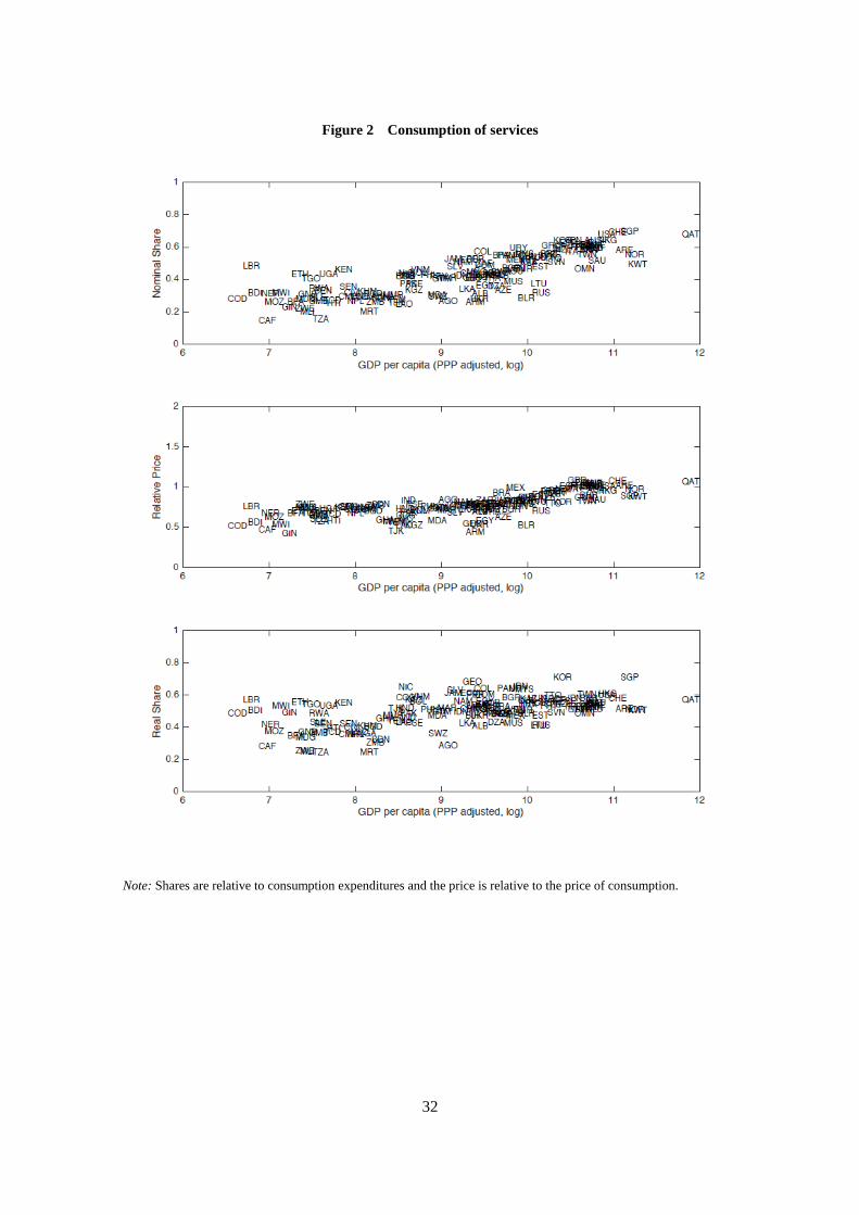
Figures 1 and 2 plot nominal and real shares of manufactured goods consumption and services in
total consumption as well as the price of manufactured goods consumption and that of services
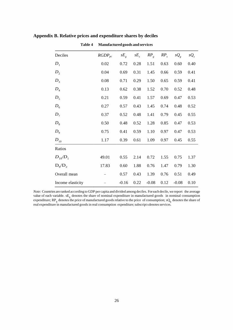
relative to the price of consumption in 2011 for all countries in our sample.9 Table 4 in
Appendix B reports average values of these variables by decile and across all countries as well as
income elasticities.10 The nominal share of manufactured goods consumption declines
systematically with income, while the share of services systematically increases with income. That
is, as countries become wealthier they tend to allocate a larger share of consumption
expenditure to services and a smaller one to manufactured goods. For example, the average
nominal share of manufactured goods in the top decile of countries in the income distribution is
39 per cent, almost half the average share in the bottom decile. The nominal share of consumption
of services in the bottom decile is 28 per cent while the average in the top decile is 61 per cent.
The relative price of manufactured goods consumption declines systematically with income,
particularly in the top half of income distribution.11 In sharp contrast, the relative price of services
8 The following exception to this allocation of categories is made: the four goods categories “Housing, Water,
Electricity, Gas, and Other Fuels” (which are “Water supply”, “Electricity,” “Gas,” and “Other Fuels”) are allocated to
services. 9 All relative prices reported in the paper are relative to the corresponding relative price of the United States. For instance,
the price of manufactured goods consumption relative to the price of consumption in any given country is normalized by the
same relative price in the United States. 10 To construct the table, countries are ranked according to real GDP per capita and divided into deciles. For each decile, the
average value of each variable is reported. The average value of each variable across all countries in the sample (“Overall
mean”) is reported as well. Each income elasticity is given by the slope coefficient from an OLS regression of the log of
each variable on log real GDP per capita across all countries in the sample. 11 The price of consumption relative to that of GDP does not vary systematically with income in this dataset. The income
elasticity of the price of consumption relative to that of GDP on log real GDP per capita, for instance, is not statistically
different from zero at the 5 per cent significance level.
10
rises systematically with income. That is, relative to the price of overall consumption, poorer
countries tend to have higher prices for manufactured goods consumption and lower prices for
services compared to wealthier countries (the top-to-bottom decile ratio is 0.72 for manufactured
goods and 1.55 for services). These facts are well known and have been documented in the
literature, both for cross-sections of countries as well as over time for individual countries.
Measuring expenditure in manufactured goods consumption and services at a common set of
international prices yields real expenditure shares, displayed in the bottom panel of Figures 1 and 2.
Qualitatively, the real shares of manufactured goods and services in consumption develop in the
same way across income as the nominal shares: the real share of manufactured goods consumption
declines with income and the real share of services increases with income. However, the
variation of the real shares across income levels is smaller than the variation of nominal shares.
That is, the shift away from manufactured goods towards services as countries become richer is
less pronounced in terms of “quantities” than in terms of nominal expenditure.12
The decomposition of consumption into manufactured goods consumption and services assigns
all goods categories to manufactured goods consumption. It should be noted, however, that it is
important to distinguish between food and non-food manufactured goods since expenditure
shares and the relative prices of these two categories of manufactured goods develop very
differently with income. The standard procedure is applied of mapping food to categories in
“Food and Non-Alcoholic Beverages” and non-food comprising all remaining categories in
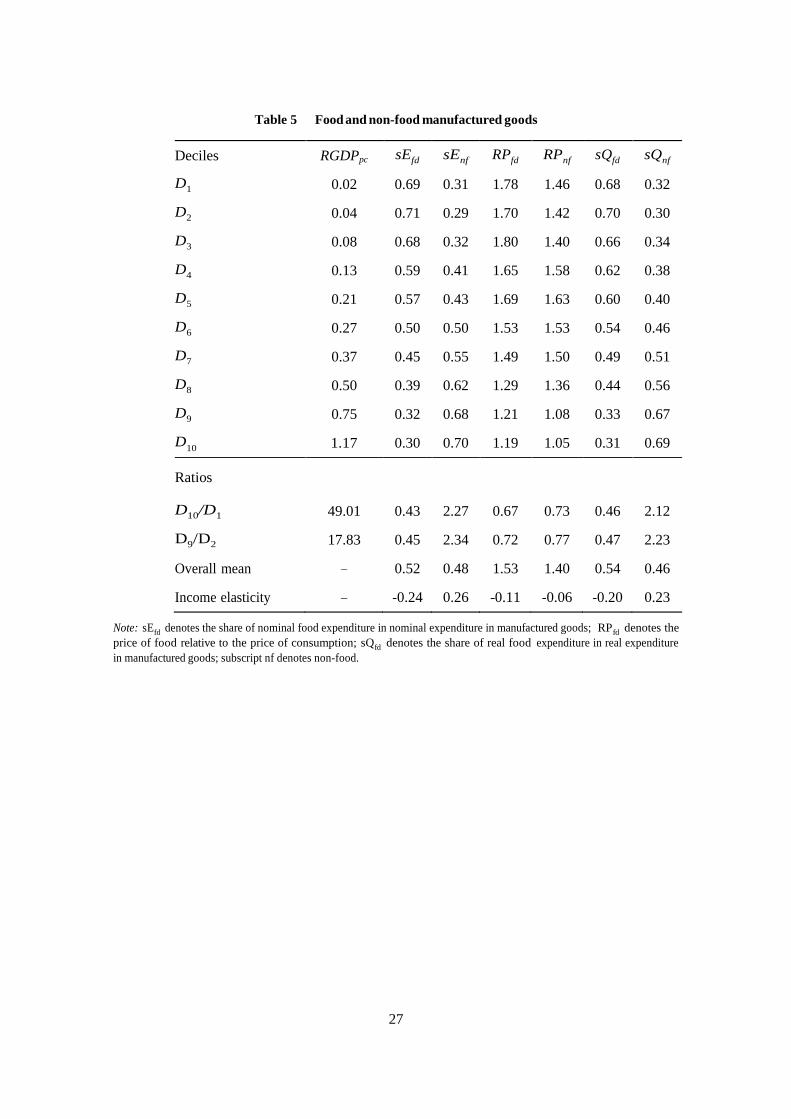
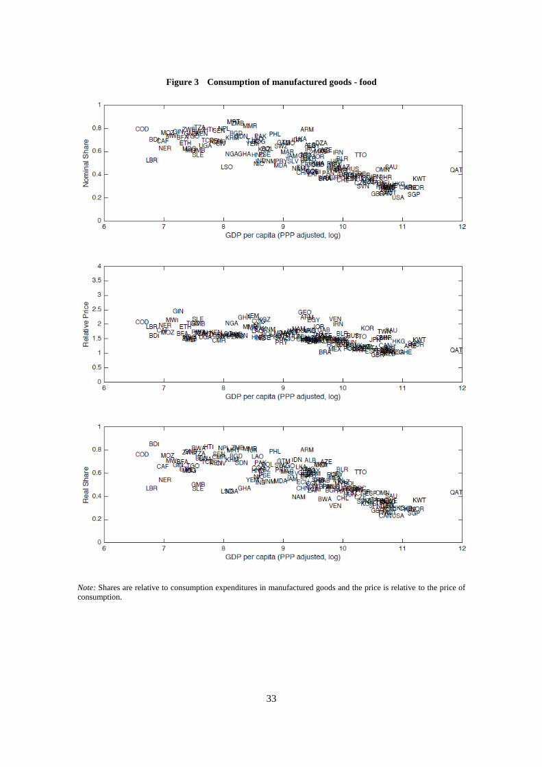
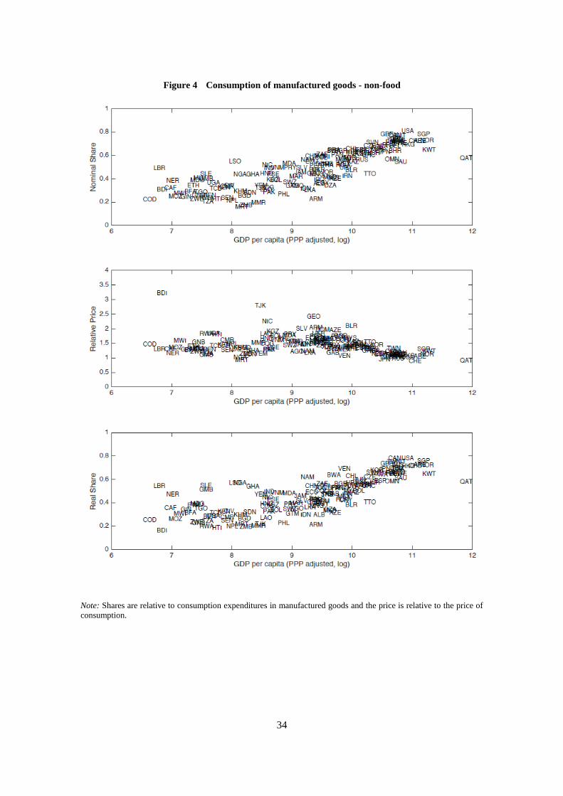
manufactured goods consumption. Figures 3 and 4 plot nominal and real shares of food and
non-food in manufactured goods consumption as well as the corresponding relative prices for all
countries in the sample. Table 5 in Appendix B reports the average values of these variables and
income elasticities. Both nominal and real shares of food in consumption expenditure on
manufactured goods decline systematically and sharply with income, particularly for the top half of
the income distribution (Figure 3). That is, richer countries tend to allocate a much smaller share
of expenditure on manufactured goods to food than poorer countries. For example, nominal
expenditure on food represents, on average, 69 per cent of nominal expenditure on manufactured
goods among countries in the bottom decile of the income distribution, while they represent only
30 per cent for countries in the top decile. Moreover, the price of food relative to that of
consumption also declines with income. The price of non-food relative to consumption, in Figure 4,
12 For manufactured goods consumption, for instance, note that both quantity (i.e. real share) and price decline with
income. Thus, nominal expenditure (price times quantity) has a more pronounced decline with income than either
price or quantity.
11
also declines systematically with income, but slightly less than the relative price of food (the top-to-
bottom decline ratio is 0.67 for the relative price of food and 0.73 for non-food).
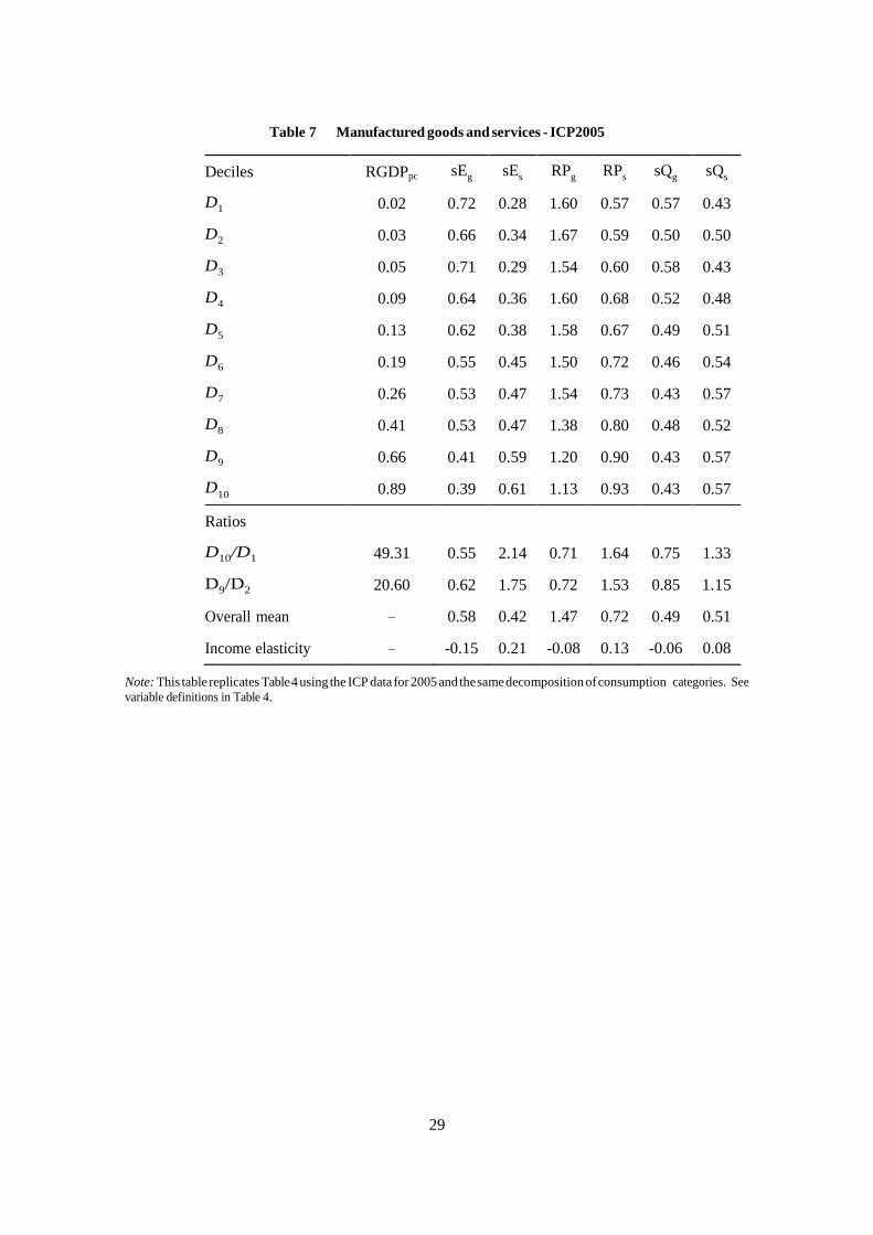
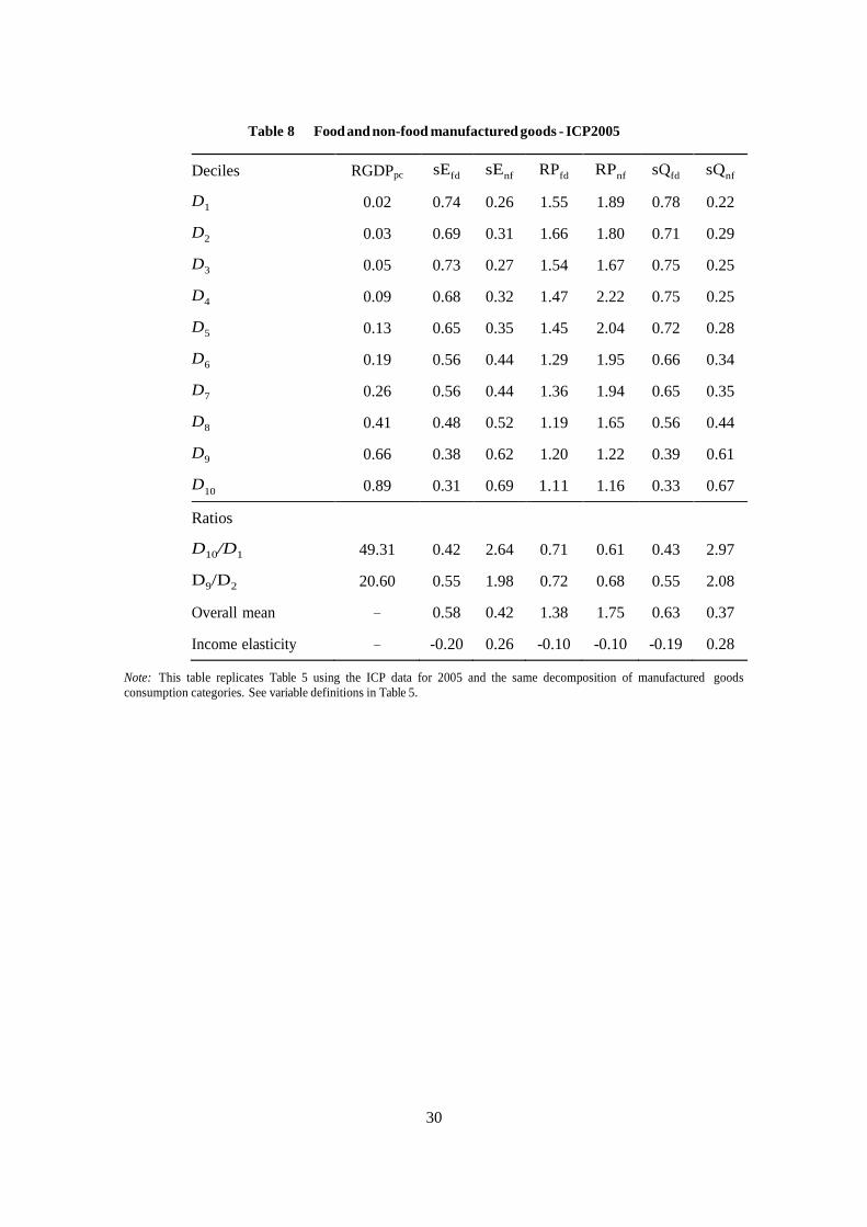
The broad decomposition of consumption expenditure on food, non-food manufactured goods and
services corresponds to the standard decomposition of consumption expenditure into sectoral
measures of economic activity (agriculture, manufacturing and services). The sectoral cross-
section patterns documented above are consistent with ICP data for other years. For instance,
Tables 7 and 8 report the average (nominal and real) shares of manufactured goods and services
in consumption, shares of food and non-food manufactured goods consumption in manufactured
goods and prices of these variables relative to that of consumption by decile using data from the
ICP dataset for 2005. Note that the two tables are quite similar to the corresponding Tables 4 and 5
obtained using the 2011 dataset. The patterns documented above are also consistent with
available evidence on the behaviour of these variables over time for individual countries. See, for
instance, evidence presented in Herrendorf et al. (2014) on consumption measures of structural
transformation.
4.2 Individual manufactured goods consumption categories
The set of manufactured consumption goods described above consists of 64 ICP individual
expenditure categories, such as “butter and margarine,” “shoes and other footwear”, “major
household appliances whether electric or not” or “motor cars”. Of these 64 categories, food
accounts for 29 categories and non-food categories for the remaining 35.13 The development of the
nominal expenditure share in the consumption of manufactured goods from these individual
categories in the cross-section of countries in the ICP is, as is to be expected, quite varied.
Nevertheless, there are many individual categories with a nominal share in manufactured
consumption that varies systematically with income. For example, “motor cars,” “audio-visual,
photographic and information processing equipment” or “major household appliances” are
individual categories for which the nominal expenditure share systematically and distinctly rises
with income. “Clothing materials, or articles of clothing and clothing accessories” is an
individual category for which this share declines systematically with income.
In terms of the development of price of each individual category of manufactured consumption
goods relative to the price of consumption, we find that it systematically declines with income for
all individual food categories, except two. For the non-food individual categories, we find that
this relative price tends to decline systematically with income for about 60 per cent of the
13 Appendix A lists the individual categories of manufactured goods consumption in the ICP data.
12
categories and to increase for the remaining ones. That is, for most individual non-food categories,
their price relative to the price of consumption tends to be lower in wealthier than in poorer
countries.14 For many of non-food categories with a relative price that declines with income, the
nominal share tends to increase systematically with income. That is, average nominal
expenditure in wealthier countries tends to be higher than in poorer countries, even though the
price of these goods tends to be lower (relative to the price of consumption). Hence, the pattern of
consumption of these categories relative to income is more pronounced when looking at real
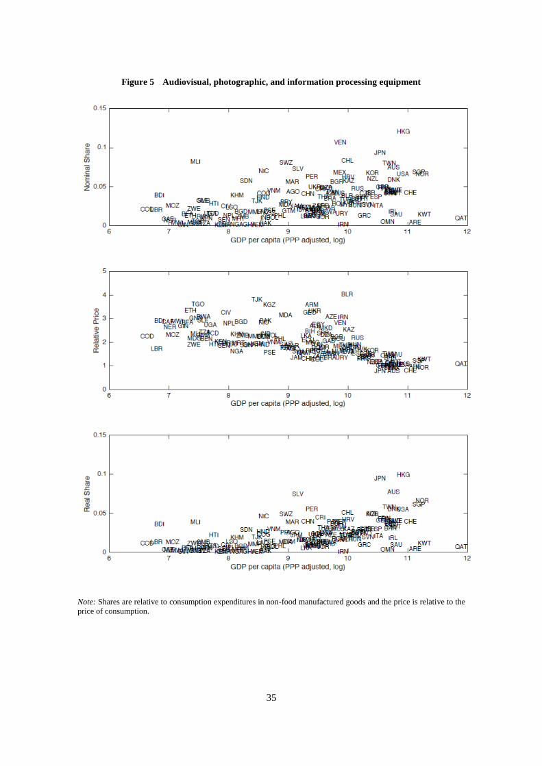
expenditure instead of nominal expenditure. Figure 5 plots these shares and the relative price of a
selected category, “audio-visual, photographic, and information processing equipment” (which
includes television and radio sets and personal computers, for example). A large variation across
income in terms of “quantities” consumed is evident, with wealthier countries allocating a larger
share of real expenditure for such goods than poorer countries. However, since the prices for
such goods tend to be relatively cheaper in richer countries, the variation across income in nominal
expenditure is lower in real expenditure.
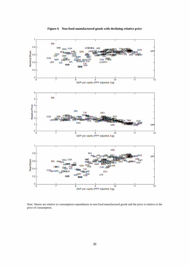
Figure 6 presents the shares and relative price for the aggregate of individual categories in non-
food manufactured consumption. A declining price relative to that of consumption is observable
as income rises. The share of nominal expenditure in the category of non-food manufactured
consumption increases systematically with income, and for the majority of countries in the top half
of income distribution, these categories represent a large share of total nominal consumption
expenditure in non-food manufactured goods. As the relative price of goods in this category
declines with income by construction, it follows that differences in expenditure shares measured
at a common set of prices between rich and poor countries are larger than the differences in
nominal shares. That is, the variation across income in expenditure shares masks a larger variation
across income in real shares.
To further characterize expenditure patterns in manufactured consumption goods across
countries, these individual categories are grouped according to different criteria. Different types of
manufactured consumption goods are grouped according to their durability. Second, goods are
grouped according to their purpose. Finally, goods are grouped based on certain assumptions on
how they are produced.
14 This finding is in sharp contrast to the heterogeneity in the development of the relative price of individual
consumption service categories reported in Duarte and Restuccia (2016).
13
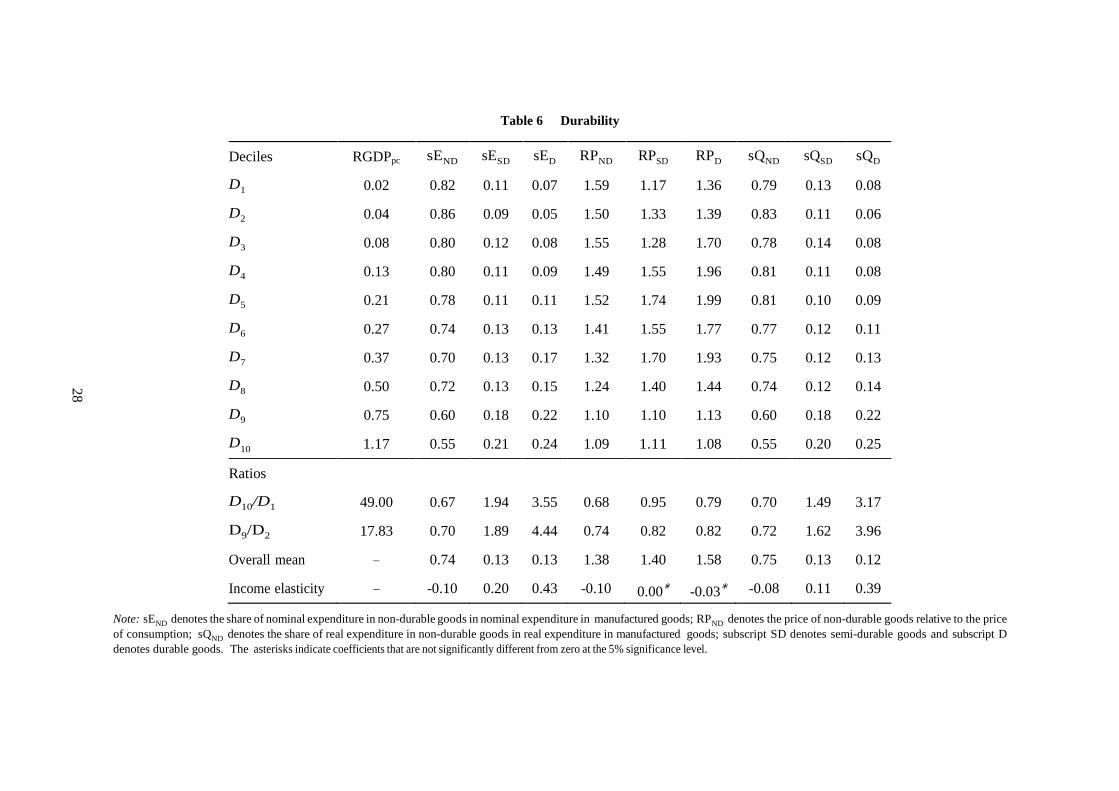
4.3 Durability and manufactured consumption
The durability attribute given to goods by COICOP are applied to each of the individual
categories included in manufactured consumption. COICOP distinguishes between durable,
semi-durable and non-durable goods. Hence, three categories of manufactured consumption
goods are constructed: “Durables” - D, “Semi-durables” - SD and “Non-durables” - ND. These
three categories represent manufactured consumption. The durability attribute of each individual
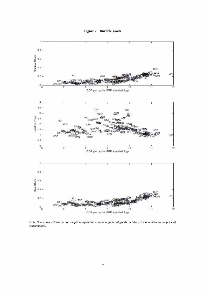
category is listed in Appendix A.15 Figures 7 to 9 plot (nominal and real) shares and the
relative price of each of these aggregates for all countries in the sample, and Table 6 in Appendix
B reports averages by decile and across all countries and income elasticities for the variable
‘interest’.
Figure 7 plots nominal and real shares of durable goods consumption in the consumption of
manufactured goods. For the countries in the bottom half of the income distribution, expenditure
(both nominal and real) in durable goods represents a very small share of total expenditure in
manufactured goods (both the real and nominal average share of expenditure in durables in
consumption expenditure in manufactured goods in the bottom decile of countries is less than
10 per cent). For the top half of the income distribution, however, the share of durable goods
consumption, both in nominal and real terms, increases systematically with income (for the top
decile, these shares average about 25 per cent). A systematic decline in the relative price of
durable goods (relative to the price of consumption) with income is also observed for the top half
of the income distribution.
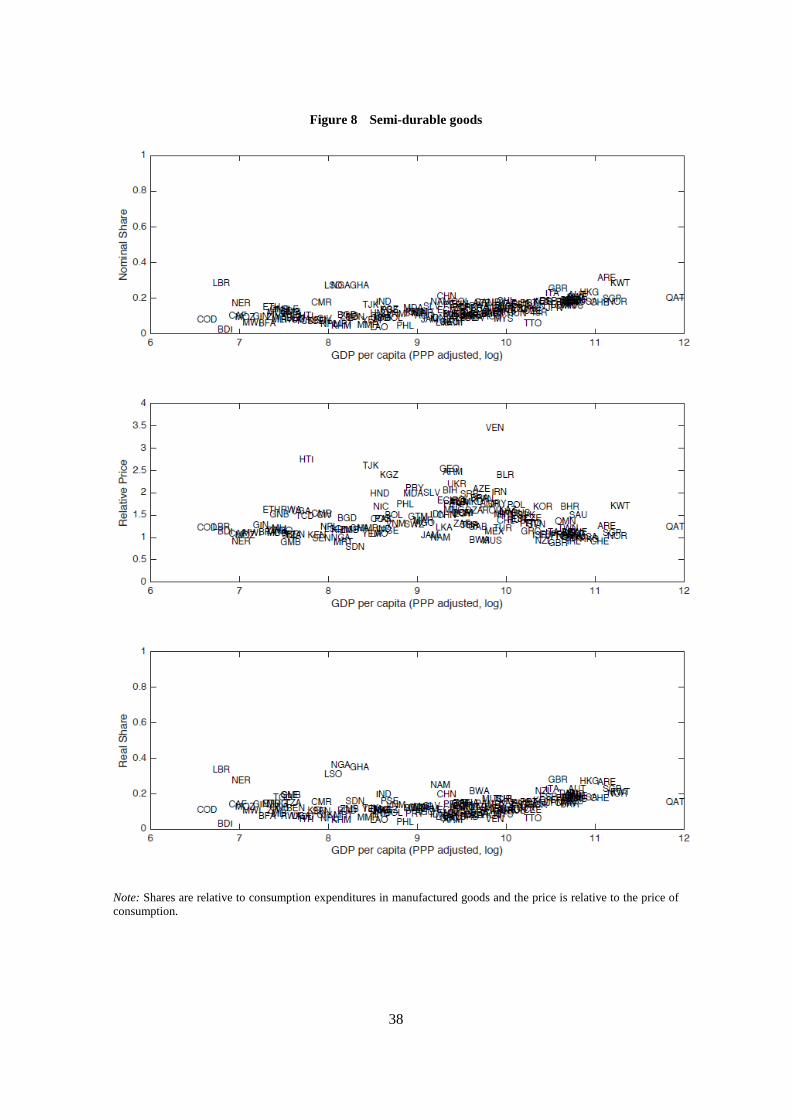
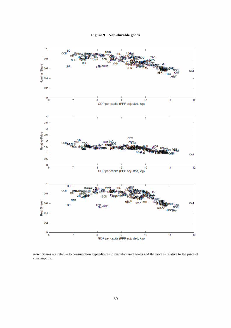
Figures 8 and 9 plot the corresponding variables for consumption of semi-durable goods and of
non-durable goods. The consumption of non-durable goods accounts by far for the largest share of
expenditure among these three categories and across the entire income distribution. For the richer
countries in the sample (in the top half of the income distribution), a lower expenditure share
in non-durable goods (both nominal and real) as income rises is associated with lower relative
prices for these goods relative to the bottom half of the distribution.
15 Note that all food categories are included in “Non-Durables”.
14
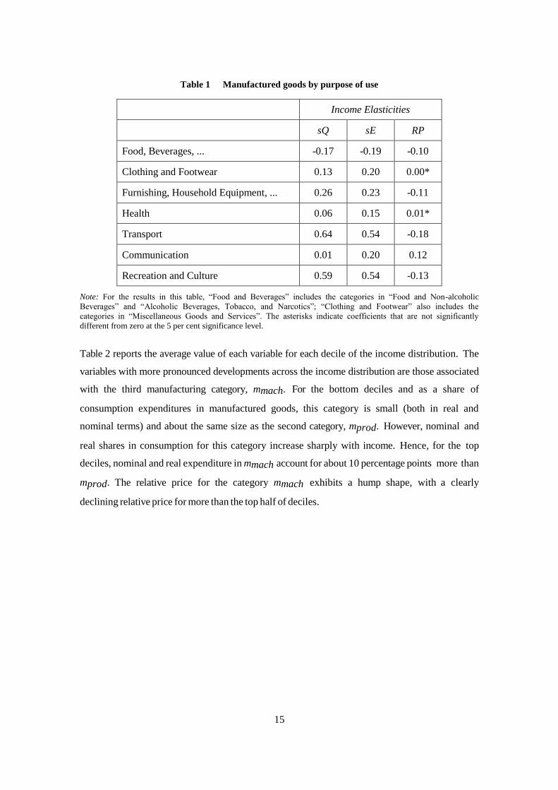
4.4 Purpose of use and manufactured consumption
Next, the consumption of manufactured goods is decomposed by the purpose of use given to
these goods. The structure of COICOP is followed, as listed in the appendix.
Table 1 reports the income elasticity of nominal and real expenditure shares of each category in
manufactured consumption expenditure as a summary statistic, as well as the income elasticity
of the price of each category relative to that of consumption. We find that most categories have
a relative price that declines with income, with the exception of “Communication.” For the
categories with a declining relative price (except “Food”), nominal expenditure increases
systematically with income, and the variation across countries in consumption shares tends to be
larger when measured in real terms (as compared to nominal terms). This finding suggests the
importance of real measures of consumption expenditure and its drives when analysing cross-
country consumption expenditure.
4.5 Decomposition by industrial classification
Finally, the categories in the consumption of manufactured goods are decomposed by establishing a
rough mapping from consumption categories to industrial categories. The manufacturing
industrial categories are divided into three, that cam broadly be described as follows: 1) industries
generally associated with the transformation of natural raw materials (e.g. the manufacture of food
products and beverages, the manufacture of textiles, of furniture, of paper, etc.)16
; 2) industries
broadly associated with the production of chemical, mineral, and metal products17
; and 3)
industries broadly associated with the manufacture of machinery18
. It must be emphasized that
this is a very rough mapping of consumption to production categories. In reality, the production
of consumption goods involves the use of different types of intermediate goods, associated with
different sectors/industries of the economy. However, this mapping provides a first step towards
deriving cross-country productivity implications from ICP consumption expenditure data. The
categories of consumption of manufactured goods allocated to the three manufacturing industrial
categories just described is as follows (the numbering in the appendix is followed here): 1)
“mraw:” 1-40, 59-61, 64; 2) “mprod:” 43-48, 54; and 3) “mmach:” 41-42, 49-53, 55-58, 62-63.
16 The associated ISIC Rev. 3 industries are 15-22 and 36. 17 The associated ISIC Rev. 3 industries are 23-28 and 40. 18 The associated ISIC Rev. 3 industries are 29-35.
15
Table 1 Manufactured goods by purpose of use
Income Elasticities
sQ sE RP
Food, Beverages, ... -0.17 -0.19 -0.10
Clothing and Footwear 0.13 0.20 0.00*
Furnishing, Household Equipment, ... 0.26 0.23 -0.11
Health 0.06 0.15 0.01*
Transport 0.64 0.54 -0.18
Communication 0.01 0.20 0.12
Recreation and Culture 0.59 0.54 -0.13
Note: For the results in this table, “Food and Beverages” includes the categories in “Food and Non-alcoholic
Beverages” and “Alcoholic Beverages, Tobacco, and Narcotics”; “Clothing and Footwear” also includes the
categories in “Miscellaneous Goods and Services”. The asterisks indicate coefficients that are not significantly
different from zero at the 5 per cent significance level.
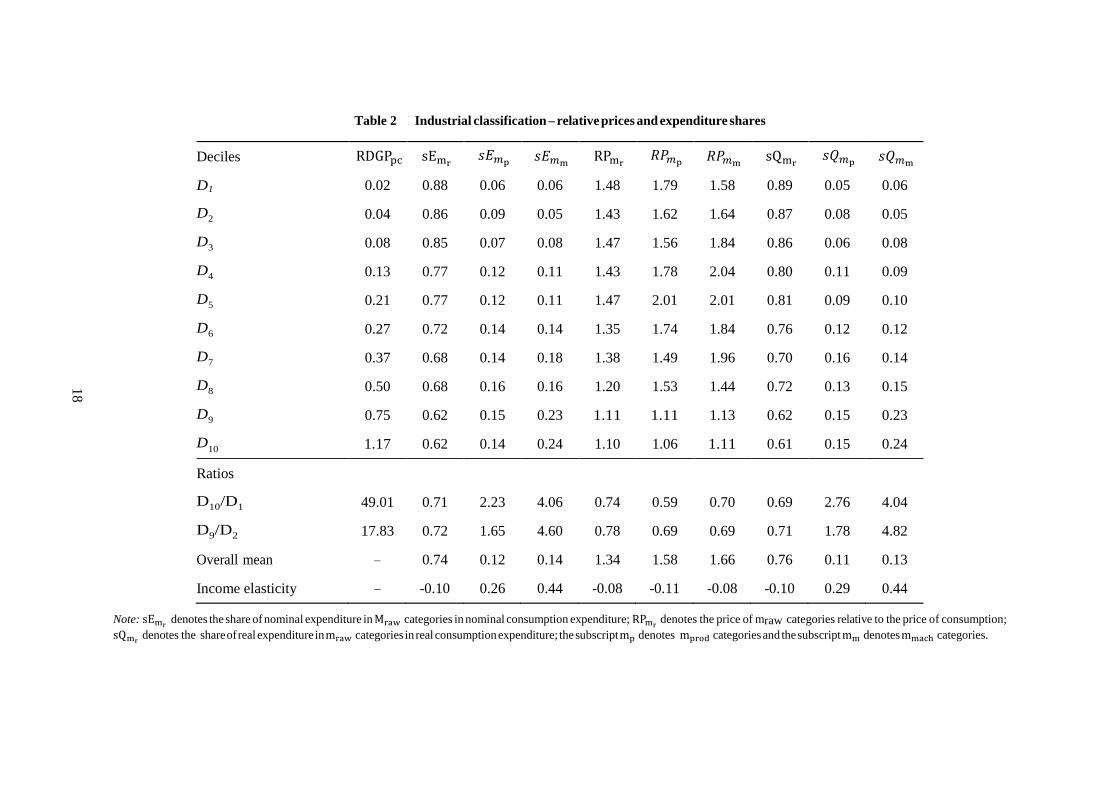
Table 2 reports the average value of each variable for each decile of the income distribution. The
variables with more pronounced developments across the income distribution are those associated
with the third manufacturing category, mmach. For the bottom deciles and as a share of
consumption expenditures in manufactured goods, this category is small (both in real and
nominal terms) and about the same size as the second category, mprod. However, nominal and
real shares in consumption for this category increase sharply with income. Hence, for the top
deciles, nominal and real expenditure in mmach account for about 10 percentage points more than
mprod. The relative price for the category mmach exhibits a hump shape, with a clearly
declining relative price for more than the top half of deciles.
16
5 Mapping to productivity
Next, a measurement of sectoral productivity differences across countries using ICP real and
nominal consumption expenditure data is carried out. Herrendorf and Valentinyi (2012) are
closely followed to conduct a development accounting exercise that imposes minimal structure.
First, the productivity implications for two sectors (manufacturing and services) are derived,
each producing a different consumption product. Next, different manufacturing sub-sectors are
considered. There are three sectors in the economy: manufacturing (m), services (s) and other
(o).19 Production in each sector is governed by linear technologies in labour, 𝑌𝑖 = 𝐴𝑖𝐿𝑖, for i ∈ {m,
s, o}, and where all variables have the interpretation given in Section 2.20
Assuming linear technologies in labour together with competitive markets for goods
and labour and perfect factor mobility across sectors implies that the value of labour
productivity is equalized across sectors and equals the wage rate w, i.e. in any given country
𝑝𝑖𝐴𝑖 = 𝑤 for all i. It follows that the value of aggregate output is ∑ 𝑝𝑖𝑌𝑖𝑖 = 𝑤𝐿, where L is
the total amount of labour in the country, and that the labour input share in each sector is
determined by the share of value output
𝐿𝑖𝐿=
𝑝𝑖𝑌𝑖
∑ 𝑝𝑖𝑌𝑖𝑖
To implement this development accounting empirically, the production function in each sector can
be written for Ai as
𝐴𝑖 =𝑌𝑖 𝐿⁄
𝐿𝑖 𝐿⁄
It is assumed that data on real expenditure per capita (Qi) represents sectoral output per unit of
labour in the model (Yi/L) and that data on the share of nominal expenditure (sEi) represents the
share value of output in each sector in the model:
(𝑝𝑖𝑌𝑖 ∑ 𝑝𝑖𝑌𝑖𝑖⁄ = 𝐿𝑖 𝐿⁄ ).
19 Sector o captures all non-consumption expenditures in the economy. 20 The objective is to measure Ai across countries. Note that the functional form for production in each sector
immediately delivers estimates of sectoral labour productivity, provided that data comparable across countries on
sectoral real output and labour exists. However, such data do not exist, at least for a comprehensive set of sectors and
for a large number of countries. Development accounting yields a measurement of cross-country sectoral labour
productivities using expenditure data and imposing minimal structure.
17
The measurement of sectoral labour productivity using real and nominal expenditure data relies on
several simplifying assumptions described above. Importantly, this measurement assumes that
sectoral real consumption expenditure maps to sectoral output, i.e. this methodology abstracts from
input-output (I-O) linkages across sectors of production. To be able to introduce I-O linkages in the
model and to derive productivity implications consistent with these, we need information on these
linkages at the level of sectoral aggregation considered in the model. There is more and more
information available on I-O tables for different countries, however, these data tend to be available
for relatively wealthier countries. That is, the set of countries for which I-O tables are available
does not cover the extreme range of income levels that characterizes the set of countries in the ICP
dataset. Therefore, there is not much evidence available on how the I-O structure varies with
income for the sectoral disaggregation considered in this paper. Duarte and Restuccia (2016)
show in a model that abstracts from the agricultural sector and food products that the I-O structure
affects the quantitative implications of a multi-sector model for sectoral labour productivity, but
leave its qualitative implications largely unchanged. Specifically, in Duarte and Restuccia (2016),
the presence of intermediate inputs reduces the ratio of productivity in manufacturing for the top
and bottom deciles of the income distribution by about a factor of two. This result follows from
the fact that a sub-set of services for which productivity gaps are very large across countries are
important intermediate inputs in the production of manufacturing goods. Therefore, by
accounting for the role of these services as inputs in manufacturing, the model implies smaller
productivity gaps in manufacturing to match the sectoral data.
18
Table 2 Industrial classification – relative prices and expenditure shares
Deciles RDGPpc sEmr 𝑠𝐸𝑚p
𝑠𝐸𝑚m RPmr
𝑅𝑃𝑚p 𝑅𝑃𝑚m
sQmr 𝑠𝑄𝑚p
𝑠𝑄𝑚m
D1 0.02 0.88 0.06 0.06 1.48 1.79 1.58 0.89 0.05 0.06
D2 0.04 0.86 0.09 0.05 1.43 1.62 1.64 0.87 0.08 0.05
D3 0.08 0.85 0.07 0.08 1.47 1.56 1.84 0.86 0.06 0.08
D4 0.13 0.77 0.12 0.11 1.43 1.78 2.04 0.80 0.11 0.09
D5 0.21 0.77 0.12 0.11 1.47 2.01 2.01 0.81 0.09 0.10
D6 0.27 0.72 0.14 0.14 1.35 1.74 1.84 0.76 0.12 0.12
D7 0.37 0.68 0.14 0.18 1.38 1.49 1.96 0.70 0.16 0.14
D8 0.50 0.68 0.16 0.16 1.20 1.53 1.44 0.72 0.13 0.15
D9 0.75 0.62 0.15 0.23 1.11 1.11 1.13 0.62 0.15 0.23
D10 1.17 0.62 0.14 0.24 1.10 1.06 1.11 0.61 0.15 0.24
Ratios
D10/D1 49.01 0.71 2.23 4.06 0.74 0.59 0.70 0.69 2.76 4.04
D9/D2 17.83 0.72 1.65 4.60 0.78 0.69 0.69 0.71 1.78 4.82
Overall mean – 0.74 0.12 0.14 1.34 1.58 1.66 0.76 0.11 0.13
Income elasticity – -0.10 0.26 0.44 -0.08 -0.11 -0.08 -0.10 0.29 0.44
Note: sEmr denotes the share of nominal expenditure in Mraw categories in nominal consumption expenditure; RPmr denotes the price of mraw categories relative to the price of consumption;
sQmr denotes the share of real expenditure in mraw categories in real consumption expenditure; the subscript mp denotes mprod categories and the subscript mm denotes mmach categories.
19
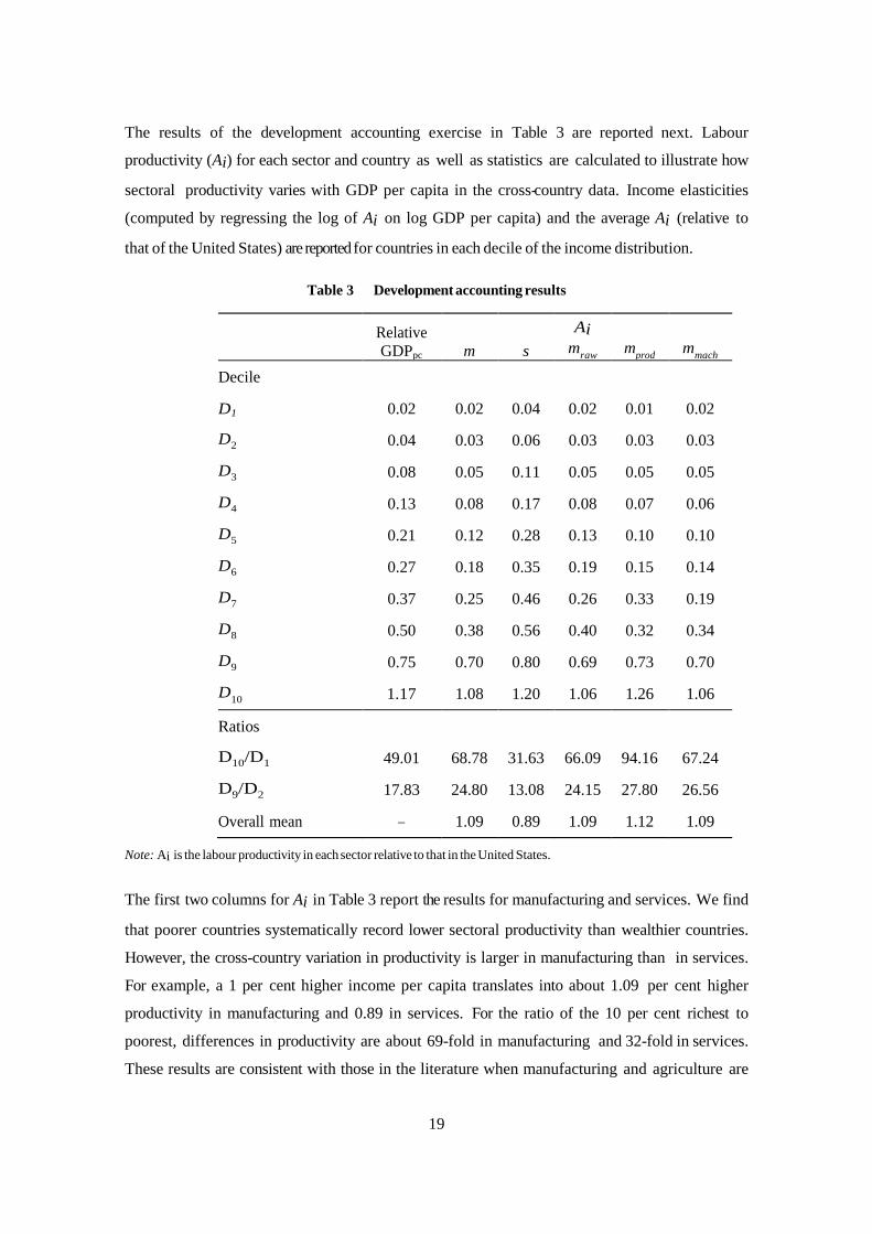
The results of the development accounting exercise in Table 3 are reported next. Labour
productivity (Ai) for each sector and country as well as statistics are calculated to illustrate how
sectoral productivity varies with GDP per capita in the cross-country data. Income elasticities
(computed by regressing the log of Ai on log GDP per capita) and the average Ai (relative to
that of the United States) are reported for countries in each decile of the income distribution.
Table 3 Development accounting results
Relative
GDPpc m s
Ai
mraw m
prod mmach
Decile
D1 0.02 0.02 0.04 0.02 0.01 0.02
D2 0.04 0.03 0.06 0.03 0.03 0.03
D3 0.08 0.05 0.11 0.05 0.05 0.05
D4 0.13 0.08 0.17 0.08 0.07 0.06
D5 0.21 0.12 0.28 0.13 0.10 0.10
D6 0.27 0.18 0.35 0.19 0.15 0.14
D7 0.37 0.25 0.46 0.26 0.33 0.19
D8 0.50 0.38 0.56 0.40 0.32 0.34
D9 0.75 0.70 0.80 0.69 0.73 0.70
D10 1.17 1.08 1.20 1.06 1.26 1.06
Ratios
D10/D1 49.01 68.78 31.63 66.09 94.16 67.24
D9/D2 17.83 24.80 13.08 24.15 27.80 26.56
Overall mean – 1.09 0.89 1.09 1.12 1.09
Note: Ai is the labour productivity in each sector relative to that in the United States.
The first two columns for Ai in Table 3 report the results for manufacturing and services. We find
that poorer countries systematically record lower sectoral productivity than wealthier countries.
However, the cross-country variation in productivity is larger in manufacturing than in services.
For example, a 1 per cent higher income per capita translates into about 1.09 per cent higher
productivity in manufacturing and 0.89 in services. For the ratio of the 10 per cent richest to
poorest, differences in productivity are about 69-fold in manufacturing and 32-fold in services.
These results are consistent with those in the literature when manufacturing and agriculture are
20
aggregated into one sector. The literature has also found considerable differences in agricultural
productivity across countries (see, for instance, Restuccia et al., 2008).21
The manufacturing sector is then disaggregated into the three sub-sectors described in Section 4.5:
mraw , mprod, and mmach. We find that there are some differences in productivity across
countries for these three sub-categories, but these are smaller than the differences between
manufacturing and services. These relatively minor differences in productivity gaps for different
manufacturing sub-sectors reflect the relatively small differences in the development of relative
prices with income for these sub-sectors. In turn, these small differences in the development of
relative prices with income at the sub-sector level reflect the fact that the heterogeneity across
individual manufacturing categories is not strongly associated with the three sub-sector
aggregation considered in this exercise. Note that, in fact, most decompositions of manufactured
goods consumption considered in the paper imply sub-sectors for which the development of relative
price is relatively homogeneous.22
Finally, we note that the category mraw includes all food categories produced in the agricultural
sector and for which there is substantial evidence of large productivity differences across
countries. Therefore, the difference in mraw also reflects the large differences in agricultural
productivity. Hence, in terms of the productivity of non-food categories, the data implies that the
largest productivity gaps occur in mmach and mprod. In terms of income elasticities, we find
that cross-country variation in productivity is largest in the manufacturing category broadly
associated with the production of chemical, mineral and metal products, mprod. That is, poorer
countries tend to be more unproductive relative to wealthier countries in these transformative
industries.
21 If the agricultural sector is mapped to food categories and manufacturing to non-food categories, we find that the
implied labour productivity differences are larger in agriculture than in manufacturing. For instance, for this
alternative definition of sectors, the top-to-bottom decile ratio is 73-fold for agriculture and 65-fold for manufacturing
and income elasticity is 1.12 for agriculture and 1.07 for manufacturing. 22 This fact reflects not only the aggregation criteria but also the fact that the heterogeneity in relative price
development across individual manufacturing consumption categories is overall smaller than the heterogeneity
across, say, individual service categories (see Duarte and Restuccia, 2016).
21
6 Conclusion
The patterns of consumption expenditure in manufactured goods across a broad set of countries
that differ in their level of development using disaggregated expenditure and price data from the
International Comparisons Program. Across broad categories, the share of consumption
expenditure in manufactured consumption goods is relatively flat while it rises for services and
falls for food as income per capita rises.
Among disaggregated manufacturing consumption categories, the patterns are quite varied with
about 60 per cent of the non-food manufactured goods categories featuring a falling relative
price and the remaining categories reveal an increasing relative price with income. The
expenditure share of non-food manufacturing categories with a falling relative price increases
systematically with income, suggesting a high degree of substitutability across non-food
manufacturing consumption categories with different degrees of productivity growth.
Expenditure and relative price patterns in manufactured consumption across countries are
characterized by grouping individual consumption categories of manufactured goods according to
different criteria.
Finally, the productivity implications associated with the decomposition of manufactured
consumption by industrial classification is explored. We find that there are some differences in
productivity across countries for these manufacturing sub-sectors, but that these differences are
smaller than those between manufacturing and services. This result largely reflects the fact that
for these sub-sectors, the development of relative price with income is relatively homogeneous.
These results suggest that the scope is not large (in terms of aggregate productivity implications)
for pursuing disaggregated industrial-level policies in the manufacturing sector.
22
References
Atkeson, Andrew, and Masao Ogaki, “Wealth-varying intertemporal elasticities of substitution:
Evidence from panel and aggregate data,” Journal of Monetary Economics, 38 (1996), 507-
534.
Baumol, William, “Macroeconomics of Unbalanced Growth: The Anatomy of Urban Crisis,”
American Economic Review, 57 (1967), 415-426.
Comin, Diego, Danial Lashkari, and Martı Mestieri, “Structural Change with Long-Run
Income and Price Effects,” manuscript (2015).
Duarte, Margarida, and Diego Restuccia, “The Role of the Structural Transformation in
Aggregate Productivity,” Quarterly Journal of Economics, 125 (2010), 129-173.
Duarte, Margarida, and Diego Restuccia, “Relative Prices and Sectoral Productivity,”
manuscript (2016).
Echevarria, Cristina, “Changes in Sectoral Composition Associated with Growth,” International
Economic Review, 38 (1997), 431-452.
Gollin, Douglas, Stephen Parente, and Richard Rogerson, “The Role of Agriculture in
Development,” American Economic Review Papers and Proceedings, 92 (2002), 160-164.
Grobovsek, Jan, “Development Accounting with Intermediate Goods,” manuscript, 2013.
Herrendorf, Berthold, Richard Rogerson, and A kos Valentinyi, “Two Perspectives on Preferences
and Structural Transformation,” American Economic Review, Vol. 103 (2013), 2752-2789.
Herrendorf, Berthold, Richard Rogerson, and
A kos Valentinyi, “Growth and Structural Transformation,” Handbook of Economic Growth, Vol.
2B (2014), 855-941.
Herrendorf, Berthold, and A kos Valentinyi, “Which Sectors Make Poor Countries so
Unproductive?,” Journal of the European Economic Association, 10 (2012), 323-341.
Heston, Alan, and Robert Summers, “International Price and Quantity Comparisons: Potentials
and Pitfalls,” American Economic Review, Vol. 86 No. 2 (1996), 20-24.
Hsieh, Chang-Tai, and Peter Klenow, “Relative Prices and Relative Prosperity,” American
Economic Review, 97 (2007), 562-585.
Kongsamut, Piyabha, Sergio Rebelo, and Danyang Xie, “Beyond Balanced Growth,” Review of
Economic Studies, 68 (2001), 869-882.
Kuznets, Simon, Modern Economic Growth. (New Haven, CT: Yale University Press, 1966).
Ngai, Rachel, and Christopher Pissarides, “Structural Change in a Multisector Model of
Growth,” American Economic Review, 97 (2007), 429-443.
Restuccia, Diego, Dennis Tao Yang, and Xiaodong Zhu, “Agriculture and Aggregate Pro-
ductivity: A Quantitative Cross-Country Analysis,” Journal of Monetary Economics, 55
(2008), 234-250.

23
Rodrick, Dani, “Premature Deindustrialization,” NBER working paper no. 20935 (2015).
Summers, Robert, and Alan Heston, “The Penn World Table: an expanded set of international
comparisons, 1950-1988,” Quarterly Journal of Economics, 106 (1991), 327-368.
24
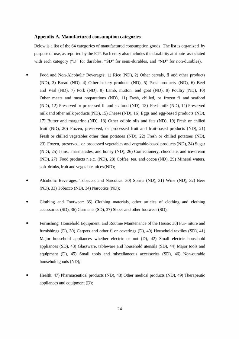
Appendix A. Manufactured consumption categories
Below is a list of the 64 categories of manufactured consumption goods. The list is organized by
purpose of use, as reported by the ICP. Each entry also includes the durability attribute associated
with each category (“D” for durables, “SD” for semi-durables, and “ND” for non-durables).
• Food and Non-Alcoholic Beverages: 1) Rice (ND), 2) Other cereals, fl and other products
(ND), 3) Bread (ND), 4) Other bakery products (ND), 5) Pasta products (ND), 6) Beef
and Veal (ND), 7) Pork (ND), 8) Lamb, mutton, and goat (ND), 9) Poultry (ND), 10)
Other meats and meat preparations (ND), 11) Fresh, chilled, or frozen fi and seafood
(ND), 12) Preserved or processed fi and seafood (ND), 13) Fresh milk (ND), 14) Preserved
milk and other milk products (ND), 15) Cheese (ND), 16) Eggs and egg-based products (ND),
17) Butter and margarine (ND), 18) Other edible oils and fats (ND), 19) Fresh or chilled
fruit (ND), 20) Frozen, preserved, or processed fruit and fruit-based products (ND), 21)
Fresh or chilled vegetables other than potatoes (ND), 22) Fresh or chilled potatoes (ND),
23) Frozen, preserved, or processed vegetables and vegetable-based products (ND), 24) Sugar
(ND), 25) Jams, marmalades, and honey (ND), 26) Confectionery, chocolate, and ice-cream
(ND), 27) Food products n.e.c. (ND), 28) Coffee, tea, and cocoa (ND), 29) Mineral waters,
soft drinks, fruit and vegetable juices (ND);
• Alcoholic Beverages, Tobacco, and Narcotics: 30) Spirits (ND), 31) Wine (ND), 32) Beer
(ND), 33) Tobacco (ND), 34) Narcotics (ND);
• Clothing and Footwear: 35) Clothing materials, other articles of clothing and clothing
accessories (SD), 36) Garments (SD), 37) Shoes and other footwear (SD);
• Furnishing, Household Equipment, and Routine Maintenance of the House: 38) Fur- niture and
furnishings (D), 39) Carpets and other fl or coverings (D), 40) Household textiles (SD), 41)
Major household appliances whether electric or not (D), 42) Small electric household
appliances (SD), 43) Glassware, tableware and household utensils (SD), 44) Major tools and
equipment (D), 45) Small tools and miscellaneous accessories (SD), 46) Non-durable
household goods (ND);
• Health: 47) Pharmaceutical products (ND), 48) Other medical products (ND), 49) Therapeutic
appliances and equipment (D);
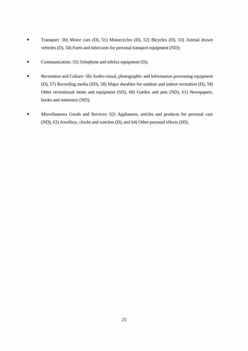
25
• Transport: 50) Motor cars (D), 51) Motorcycles (D), 52) Bicycles (D), 53) Animal drawn
vehicles (D), 54) Fuels and lubricants for personal transport equipment (ND);
• Communication: 55) Telephone and telefax equipment (D);
• Recreation and Culture: 56) Audio-visual, photographic and information processing equipment
(D), 57) Recording media (SD), 58) Major durables for outdoor and indoor recreation (D), 59)
Other recreational items and equipment (SD), 60) Garden and pets (ND), 61) Newspapers,
books and stationery (ND);
• Miscellaneous Goods and Services: 62) Appliances, articles and products for personal care
(ND), 63) Jewellery, clocks and watches (D), and 64) Other personal effects (SD).
26
Appendix B. Relative prices and expenditure shares by deciles
Table 4 Manufactured goods and services
Deciles RGDPpc sEg sEs RPg RPs sQg sQs
D1 0.02 0.72 0.28 1.51 0.63 0.60 0.40
D2 0.04 0.69 0.31 1.45 0.66 0.59 0.41
D3 0.08 0.71 0.29 1.50 0.65 0.59 0.41
D4 0.13 0.62 0.38 1.52 0.70 0.52 0.48
D5 0.21 0.59 0.41 1.57 0.69 0.47 0.53
D6 0.27 0.57 0.43 1.45 0.74 0.48 0.52
D7 0.37 0.52 0.48 1.41 0.79 0.45 0.55
D8 0.50 0.48 0.52 1.28 0.85 0.47 0.53
D9 0.75 0.41 0.59 1.10 0.97 0.47 0.53
D10 1.17 0.39 0.61 1.09 0.97 0.45 0.55
Ratios
D10/D1 49.01 0.55 2.14 0.72 1.55 0.75 1.37
D9/D2 17.83 0.60 1.88 0.76 1.47 0.79 1.30
Overall mean – 0.57 0.43 1.39 0.76 0.51 0.49
Income elasticity – -0.16 0.22 -0.08 0.12 -0.08 0.10
Note: Countries are ranked according to GDP per capita and divided among deciles. For each decile, we report the average
value of each variable. sEg denotes the share of nominal expenditure in manufactured goods in nominal consumption
expenditure; RPg denotes the price of manufactured goods relative to the price of consumption; sQg denotes the share of
real expenditure in manufactured goods in real consumption expenditure; subscript s denotes services.
27
Table 5 Food and non-food manufactured goods
Deciles RGDPpc sEfd sEnf RPfd RPnf sQfd sQnf
D1 0.02 0.69 0.31 1.78 1.46 0.68 0.32
D2 0.04 0.71 0.29 1.70 1.42 0.70 0.30
D3 0.08 0.68 0.32 1.80 1.40 0.66 0.34
D4 0.13 0.59 0.41 1.65 1.58 0.62 0.38
D5 0.21 0.57 0.43 1.69 1.63 0.60 0.40
D6 0.27 0.50 0.50 1.53 1.53 0.54 0.46
D7 0.37 0.45 0.55 1.49 1.50 0.49 0.51
D8 0.50 0.39 0.62 1.29 1.36 0.44 0.56
D9 0.75 0.32 0.68 1.21 1.08 0.33 0.67
D10 1.17 0.30 0.70 1.19 1.05 0.31 0.69
Ratios
D10/D1 49.01 0.43 2.27 0.67 0.73 0.46 2.12
D9/D2 17.83 0.45 2.34 0.72 0.77 0.47 2.23
Overall mean – 0.52 0.48 1.53 1.40 0.54 0.46
Income elasticity – -0.24 0.26 -0.11 -0.06 -0.20 0.23
Note: sEfd denotes the share of nominal food expenditure in nominal expenditure in manufactured goods; RPfd denotes the
price of food relative to the price of consumption; sQfd denotes the share of real food expenditure in real expenditure
in manufactured goods; subscript nf denotes non-food.
28
Table 6 Durability
Deciles RGDPpc sEND sESD sED RPND RPSD RPD sQND sQSD sQD
D1 0.02 0.82 0.11 0.07 1.59 1.17 1.36 0.79 0.13 0.08
D2 0.04 0.86 0.09 0.05 1.50 1.33 1.39 0.83 0.11 0.06
D3 0.08 0.80 0.12 0.08 1.55 1.28 1.70 0.78 0.14 0.08
D4 0.13 0.80 0.11 0.09 1.49 1.55 1.96 0.81 0.11 0.08
D5 0.21 0.78 0.11 0.11 1.52 1.74 1.99 0.81 0.10 0.09
D6 0.27 0.74 0.13 0.13 1.41 1.55 1.77 0.77 0.12 0.11
D7 0.37 0.70 0.13 0.17 1.32 1.70 1.93 0.75 0.12 0.13
D8 0.50 0.72 0.13 0.15 1.24 1.40 1.44 0.74 0.12 0.14
D9 0.75 0.60 0.18 0.22 1.10 1.10 1.13 0.60 0.18 0.22
D10 1.17 0.55 0.21 0.24 1.09 1.11 1.08 0.55 0.20 0.25
Ratios
D10/D1 49.00 0.67 1.94 3.55 0.68 0.95 0.79 0.70 1.49 3.17
D9/D2 17.83 0.70 1.89 4.44 0.74 0.82 0.82 0.72 1.62 3.96
Overall mean – 0.74 0.13 0.13 1.38 1.40 1.58 0.75 0.13 0.12
Income elasticity – -0.10 0.20 0.43 -0.10 0.00∗ -0.03∗ -0.08 0.11 0.39
Note: sEND denotes the share of nominal expenditure in non-durable goods in nominal expenditure in manufactured goods; RPND denotes the price of non-durable goods relative to the price
of consumption; sQND denotes the share of real expenditure in non-durable goods in real expenditure in manufactured goods; subscript SD denotes semi-durable goods and subscript D
denotes durable goods. The asterisks indicate coefficients that are not significantly different from zero at the 5% significance level.
29
Table 7 Manufactured goods and services - ICP2005
Deciles RGDPpc sEg sEs RPg RPs sQg sQs
D1 0.02 0.72 0.28 1.60 0.57 0.57 0.43
D2 0.03 0.66 0.34 1.67 0.59 0.50 0.50
D3 0.05 0.71 0.29 1.54 0.60 0.58 0.43
D4 0.09 0.64 0.36 1.60 0.68 0.52 0.48
D5 0.13 0.62 0.38 1.58 0.67 0.49 0.51
D6 0.19 0.55 0.45 1.50 0.72 0.46 0.54
D7 0.26 0.53 0.47 1.54 0.73 0.43 0.57
D8 0.41 0.53 0.47 1.38 0.80 0.48 0.52
D9 0.66 0.41 0.59 1.20 0.90 0.43 0.57
D10 0.89 0.39 0.61 1.13 0.93 0.43 0.57
Ratios
D10/D1 49.31 0.55 2.14 0.71 1.64 0.75 1.33
D9/D2 20.60 0.62 1.75 0.72 1.53 0.85 1.15
Overall mean – 0.58 0.42 1.47 0.72 0.49 0.51
Income elasticity – -0.15 0.21 -0.08 0.13 -0.06 0.08
Note: This table replicates Table 4 using the ICP data for 2005 and the same decomposition of consumption categories. See
variable definitions in Table 4.
30
Table 8 Food and non-food manufactured goods - ICP2005
Deciles RGDPpc sEfd sEnf RPfd RPnf sQfd sQnf
D1 0.02 0.74 0.26 1.55 1.89 0.78 0.22
D2 0.03 0.69 0.31 1.66 1.80 0.71 0.29
D3 0.05 0.73 0.27 1.54 1.67 0.75 0.25
D4 0.09 0.68 0.32 1.47 2.22 0.75 0.25
D5 0.13 0.65 0.35 1.45 2.04 0.72 0.28
D6 0.19 0.56 0.44 1.29 1.95 0.66 0.34
D7 0.26 0.56 0.44 1.36 1.94 0.65 0.35
D8 0.41 0.48 0.52 1.19 1.65 0.56 0.44
D9 0.66 0.38 0.62 1.20 1.22 0.39 0.61
D10 0.89 0.31 0.69 1.11 1.16 0.33 0.67
Ratios
D10/D1 49.31 0.42 2.64 0.71 0.61 0.43 2.97
D9/D2 20.60 0.55 1.98 0.72 0.68 0.55 2.08
Overall mean – 0.58 0.42 1.38 1.75 0.63 0.37
Income elasticity – -0.20 0.26 -0.10 -0.10 -0.19 0.28
Note: This table replicates Table 5 using the ICP data for 2005 and the same decomposition of manufactured goods
consumption categories. See variable definitions in Table 5.
31
Figure 1 Consumption of manufactured goods
Note: Shares are relative to consumption expenditures and the price is relative to the price of consumption.
32
Figure 2 Consumption of services
Note: Shares are relative to consumption expenditures and the price is relative to the price of consumption.
33
Figure 3 Consumption of manufactured goods - food
Note: Shares are relative to consumption expenditures in manufactured goods and the price is relative to the price of
consumption.
34
Figure 4 Consumption of manufactured goods - non-food
Note: Shares are relative to consumption expenditures in manufactured goods and the price is relative to the price of
consumption.
35
Figure 5 Audiovisual, photographic, and information processing equipment
Note: Shares are relative to consumption expenditures in non-food manufactured goods and the price is relative to the
price of consumption.
36
Figure 6 Non-food manufactured goods with declining relative price
Note: Shares are relative to consumption expenditures in non-food manufactured goods and the price is relative to the
price of consumption.
37
Figure 7 Durable goods
Note: Shares are relative to consumption expenditures in manufactured goods and the price is relative to the price of
consumption.
38
Figure 8 Semi-durable goods
Note: Shares are relative to consumption expenditures in manufactured goods and the price is relative to the price of
consumption.
39
Figure 9 Non-durable goods
Note: Shares are relative to consumption expenditures in manufactured goods and the price is relative to the price of
consumption.

Vienna International Centre · P.O. Box 300 9 · 1400 Vienna · AustriaTel.: (+43-1) 26026-o · E-mail: [email protected]