Embed Size (px)
Citation preview

University of Georgia, Athens, USA. First released May 12, 2014 Last edit May 3, 2018
Manual for
BLUPF90 family of programs
Ignacy Misztal ([email protected]), Shogo Tsuruta ([email protected]),
Daniela Lourenco ([email protected]), Yutaka Masuda ([email protected])
University of Georgia, USA
Ignacio Aguilar ([email protected])
INIA, Uruguay
Andres Legarra ([email protected])
INRA Toulouse, France
Zulma Vitezica ([email protected])
ENSAT, France

2
Table of Contents
Introduction ............................................................................................................................................ 4
List of programs from Wiki page ..................................................................................................... 5
Programs in a chart .............................................................................................................................. 6
Parameter file for application programs ...................................................................................... 7
Description of effects .................................................................................................................................... 8
Definition of random effects ....................................................................................................................... 10
Correlated effects .................................................................................................................................... 11
Data and Pedigree files ........................................................................................................................... 14
Data file ................................................................................................................................................... 14
Pedigree file ............................................................................................................................................ 14
Error messages in parameter file ............................................................................................................ 14
RENUMF90 parameter file .......................................................................................................................... 15
Basic rules for RENUMF90 parameter file............................................................................................... 15
Parameter file ......................................................................................................................................... 15
Combining fields ...................................................................................................................................... 17
Options .................................................................................................................................................... 17
Output files .............................................................................................................................................. 17
Output pedigree file ................................................................................................................................ 18
Example ................................................................................................................................................... 18
When to use what program and computing limits .................................................................. 22
BLUP ............................................................................................................................................................ 22
Variance component estimation ................................................................................................................ 24
Genomic programs ...................................................................................................................................... 32
PREGSF90 ................................................................................................................................................ 32
POSTGSF90 .............................................................................................................................................. 39
PREDF90 .................................................................................................................................................. 41
Demonstration for genomic analysis ...................................................................................................... 42
PREDICTF90 ............................................................................................................................................. 44
Examples for parameter files .......................................................................................................... 47
Appendix A (single trait animal model) ...................................................................................... 63
Appendix B (multiple trait sire model) ....................................................................................... 67
Appendix C (test-day model) ........................................................................................................... 70
Appendix D (multibreed maternal effect model) .................................................................... 74
Appendix E (random regression model)..................................................................................... 77
Appendix F (terminal cross model) .............................................................................................. 79

3
Appendix G (competitive model) ................................................................................................... 81
Appendix H (genomic model) ......................................................................................................... 83
Appendix I (complete genomic analysis) .................................................................................... 94
Appendix J (custom relationship matrices) ............................................................................ 123
Appendix K (selected programming details) ......................................................................... 125
Modules and Libraries .................................................................................................................... 128
Module DENSEOP ..................................................................................................................................... 128
Symmetric matrices............................................................................................................................... 128
General matrices ................................................................................................................................... 129
Technical details .................................................................................................................................... 129
Example (exdense.f90) .......................................................................................................................... 130
Compilation ........................................................................................................................................... 130
Module SPARSEM ..................................................................................................................................... 131
Introduction........................................................................................................................................... 131
Matrix formats ...................................................................................................................................... 132
Matrix operations ................................................................................................................................. 132
Storage type .......................................................................................................................................... 134
Numerical accuracy ............................................................................................................................... 134
Diagnostics ............................................................................................................................................ 134
FSPAK90 ................................................................................................................................................ 134
Module Prob ............................................................................................................................................. 141
Subroutines/functions ........................................................................................................................... 141
Other functions/subroutines ................................................................................................................. 142

4
Introduction
BLUPF90 is a family of programs for mixed-model computations with focus on animal breeding
applications. The programs can do data conditioning, estimate variances using several methods,
calculate BLUP for very large data sets, calculate approximate accuracy, and use SNP information for
improved accuracy of breeding values + for genome-wide association studies (GWAS).
The programs have been designed with 3 goals in mind:
1. Flexibility to support a large set of models found in animal breeding applications.
2. Simplicity of software to minimize errors and facilitate modifications.
3. Efficiency at the algorithmic level.
Aside from being used in hundreds of studies, the programs are utilized for commercial genetic
evaluation in dairy, beef, pigs and broiler chicken by major companies/institutions/associations in the US
and beyond.
The programs are written in Fortran 90/95 and originated as exercises for a class taught by Ignacy
Misztal at the University of Georgia. Over time, they have been upgraded and enhanced by many
contributors. Details on programming and computing algorithms are available in an Interbull 1999 paper
and as course notes. Nearly all programs are available in source code.
Online information about the programs is available at http://nce.ads.uga.edu/wiki/doku.php as wiki
pages. There is discussion group blupf90 at groups.yahoo.com.

5
List of programs from Wiki page
Latest versions available from website at
http://nce.ads.uga.edu/wiki/doku.php?id=application_programs
(Use latest versions. All applications for Linux, Mac OSX, and Windows have been updated frequently)
The programs support mixed models with multiple-correlated effects, multiple animal models and dominance.
▪ BLUPF90 - BLUP in memory
▪ REMLF90 - accelerated EM REML
▪ QXPAK - joint analysis of QTL and polygenic effects (M. Perez-Enciso) QxPak web page
▪ AIREMLF90 - Average Information REML with several options including EM-REML and heterogeneous residual
variances (S. Tsuruta)
▪ CBLUP90 - solutions for bivariate linear-threshold models
▪ CBLUP90THR - as above but with thresholds computed and many linear traits (B. Auvray)
▪ CBLUP90REML - as above but with quasi REML (B. Auvray)
▪ GIBBSF90 - simple block implementation of Gibbs sampling
▪ GIBBS1F90 - as above but faster for creating mixed model equations only once
▪ GIBBS2F90 - as above but with joint sampling of correlated effects
▪ GIBBS3F90 - as above with support for heterogeneous residual variances
▪ POSTGIBBSF90 - statistics and graphics for post-Gibbs analysis (S. Tsuruta)
▪ THRGIBBSF90 - Gibbs sampling for any combination of categorical and linear traits (D. Lee)
▪ THRGIBBS1F90 - as above but simplified with several options (S. Tsuruta)
▪ RENUMF90 - a renumbering program that also can check pedigrees and assign unknown parent groups; supports
large data sets
▪ INBUPGF90 - a program to calculate inbreeding coefficients with incomplete pedigree (I. Aguilar)
▪ SEEKPARENTF90 - a program to verify paternity and parent discovery using SNP markers (I. Aguilar)
▪ PREDICTF90 - a program to calculate adjusted y, �̂�, and residuals (I. Aguilar)
▪ PREDF90 - a program to predict direct genomic value (DGV) for animals based on genotypes and SNP solution
Available by request
▪ MRF90 - Method R program suitable for very large data sets; contact T. Druet.
▪ COXF90 – Bayesian Cox model - contact J. P. Sanchez ([email protected])
▪ BLUPF90HYP – BLUPF90 with hypothesis testing (F and Chi2 tests) - contact J. P. Sanchez as above
Available only under research agreement
▪ BLUP90IOD2 - BLUP by iteration on data with support for very large models (S. Tsuruta)
▪ CBLUP90IOD - BLUP by iteration on data for threshold-linear models
▪ ACCF90 - approximation of accuracies for breeding values
▪ BLUP90MBE - BLUP by iteration on data with support for very large models for multi-breed evaluations
▪ BLUP90ADJ - BLUP data preadjustment tool
Included in application programs
▪ PREGSF90 – genomic preprocessor that combines genomic and pedigree relationships (I. Aguilar)
▪ POSTGSF90 – genomic postprocessor that extracts SNP solutions after genomic evaluations (single step, GBLUP)
(I. Aguilar)
Other programming contributions were made by Miguel Perez-Enciso (user_file) and François Guillaume
(Jenkins hashing functions).

6
Programs in a chart
Application programs (BLUP*, *REMLF90, THRGIBBS*, and GIBBS*) are driven by parameter files and
require data files with effects renumbered from 1 consecutively.
Renumbering and quality control can be done by RENUMF90, which is also driven by a parameter file.
Separation of renumbering and application programs allows supporting complicated models.
Some models are not directly supported by RENUMF90 and require tweaking the parameter file in the
application programs.

7
Parameter file for application programs
The parameter file has keywords that are fixed and cannot be changed followed by values, with the
following structure (the following example comes from 2-trait maternal model):
Keywords* Description DATAFILE Name of file with phenotypes; free fortran format (space-delimited file)
file.dat
NUMBER OF TRAITS Number of traits
2
NUMBER OF EFFECTS Number of effects in a model except for residual
6
OBSERVATIONS(S) Position(s) of observations in data file
1 2
WEIGHTS
2
Position of weight on observations if used; otherwise blank
“2” means that residual variance (R) is set to R/2.
EFFECTS: POSITIONS_IN_DATAFILE NUMBER_OF_LEVELS TYPE_OF_EFFECT [EFFECT NESTED]
4 4 10 cross 4 4 = crossclassified effect positions in data file for 2 traits; 10 = levels
5 0 100 cross 5 0 = crossclassified effect, positions for 2 traits; 100 = levels
6 6 1 cov 6 6 = covariable positions in data file
7 7 10 cov 4 4 7 7 = covariable nested in effect position 4; 10 = levels
8 8 1000 cross 8 8 = crossclassified effect positions for 2 traits; 1000 = levels
0 9 1000 cross 0 9 = crossclassified effect positions for 2 traits; 1000 = levels
RANDOM_RESIDUAL_VALUES Residual variance or residual covariance matrix
10 1
1 10
For 2 trait model
RANDOM_GROUP List of effect numbers that form a group
5 6 For correlated random effects 5 6
RANDOM_TYPE Type of random effect (distribution)
add_animal diagonal, add_sire, add_an_upg, add_an_upginb, par_domin, or user_file
FILE Pedigree file or other file associated with random effect; blank if none
file.ped
(CO)VARIANCES (Co)variance matrix for each random effect
10 1 0 1
1 10 0 1
0 0 0 0
1 1 0 10
For 2 trait model
*Keywords need to be typed exactly (up to 20 characters). When preparing a new parameter file,
consider modifying an existing file.
Note that this parameter file is for application programs (BLUPF90, AIREMLF90, GIBBSF90 etc.) and it is
not for RENUMF90. This program needs a different type of parameter file. See page 15 for details.

8
Description of effects
The effects are specified after the keyword:
EFFECTS: POSITIONS_IN_DATAFILE NUMBER_OF_LEVELS TYPE_OF_EFFECT [EFFECT NESTED]
Each line contains the following:
- Position(s) of each effect in the data file; t positions for t traits
- Number of levels (assumed consecutive from 1)
- Type of effect: “cross” for crossclassified, and “cov” for covariable
o crossclassified uses integer number from 1
o covariable uses integer or real numbers
- For nested covariables, the following number (or t numbers for t traits) indicates the position of
nesting in the data file
- Text after # can be used as a comment
Consider a data file (file.dat) with the following columns
i j k y1 y2 x1
2 2 3 4.30 5.67 22.40
1 2 2 2.76 3.20 18.00
…………………………………
3 1 1 2.20 5.30 7.25
Let i go from 1 to 50, j from 1 to 80, and k from 1 to 200. The model:
y1ij=aj+bi+cX+eij
will be specified in the parameter file as:
DATAFILE
file.dat
NUMBER_OF_TRAITS
1
NUMBER_OF_EFFECTS
3
OBSERVATIONS(S)
4
WEIGHTS
EFFECTS: POSITIONS_IN_DATAFILE NUMBER_OF_LEVELS TYPE_OF_EFFECT [EFFECT NESTED]
2 80 cross # position 2, 80 levels
1 50 cross # position 1, 50 levels
6 1 cov # covariable on position 6, one level
……
By definition, a regular covariable has one level (i.e., a slope as regression).
9
For a similar model but with a nested covariable:
y1ij=aj+bi+ciX+eij
The description will change to:
EFFECTS: POSITIONS_IN_DATAFILE NUMBER_OF_LEVELS TYPE_OF_EFFECT [EFFECT NESTED]
2 80 cross # position 2, 80 levels
1 50 cross # position 1, 50 levels
6 50 cov 1 # covariable on position 6 nested in position 1; 50 levels
Assume a two trait model:
y1ij=a1j+ c1iX+e1ij
y2ij= b2i+c2iX+e2ij
This corresponds to: ……
NUMBER_OF_TRAITS
2
NUMBER_OF_EFFECTS
3
……
EFFECTS: POSITIONS_IN_DATAFILE NUMBER_OF_LEVELS TYPE_OF_EFFECT [EFFECT NESTED]
2 0 80 cross # position 2 for trait 1 only, 80 levels
0 1 50 cross # position 1 for trait 2 only, 50 levels
6 6 50 cov 1 1 # covariable on position 6 for two traits nested in position 1
“0” in effect definitions means missing effect per trait.
Two effects above can be merged:
NUMBER_OF_EFFECTS
2
……
EFFECTS: POSITIONS_IN_DATAFILE NUMBER_OF_LEVELS TYPE_OF_EFFECT [EFFECT NESTED]
2 1 80 cross # positions 2 and 1 for traits 1 and 2, 80 is max(50,80)levels
6 6 50 cov 1 1 # covariable on position 6 for two traits nested in position 1
10
Definition of random effects
RANDOM_GROUP defines one group of random effects. A group is one effect or multiple (correlated)
effects that share the same covariance structure, e.g., direct-maternal effect or random regressions.
The structure of RANDOM GROUP is:
RANDOM_GROUP 5 or 5 6
Corresponding to the effect number specified above; “5” means that the 5th effect is random. Or “5 6” means that 5th and 6th are correlated random effects.
RANDOM_TYPE defines a covariance structure: diagonal var() = s I or G where s is a variance and G is
a covariance matrix. For other types, see “Random effects and Pedigree files”
Assume a model:
y = farm + animal_additive + animal_environment + error
with var(animal_additive) = 2.5A, var(animal_environment) = 5.1I, var(error) = 13.7I
With these effects: EFFECTS: POSITIONS_IN_DATAFILE NUMBER_OF_LEVELS TYPE_OF_EFFECT [EFFECT NESTED]
3 100 cross # effect 1: farm
2 1000 cross # effect 2: additive genetic
2 1000 cross # effect 3: permanent environment
RANDOM_RESIDUAL_VALUES
13.7
RANDOM_GROUP
2 # this is for effect 2 on the effect list
RANDOM_TYPE
add_animal # additive genetic
FILE
file.ped # name of pedigree file
(CO)VARIANCES
2.5
RANDOM_GROUP
3 # effect 3 on the effect list above
RANDOM_TYPE
diagonal # permanent environment
FILE
# no file associated with diagonal structures
(CO)VARIANCES
5.1
11
Correlated effects
Assume a model:
y = farm + season + direct + maternal + error
var(direct,maternal)= [5 11 6
]⨂ A
with the effects as specified:
EFFECTS: POSITIONS_IN_DATAFILE NUMBER_OF_LEVELS TYPE_OF_EFFECT [EFFECT NESTED]
3 100 cross # effect 1: farm
4 4 cross # effect 2: season
2 1000 cross # effect 3: direct
2 1000 cross # effect 3: maternal
The distribution of the random effects are specified below:
…
RANDOM_GROUP
3 4 # direct and maternal effects
RANDOM_TYPE
add_animal # additive genetic
FILE
file.ped # name of pedigree file
(CO)VARIANCES
5 1
1 6
…
Random regression models may have many correlated random effects. Assume a data file with the
following positions:
1 to 4: polynomials
5: animal number (1000 levels)
6: herd year season (50 levels) …
EFFECTS: POSITIONS_IN_DATAFILE NUMBER_OF_LEVELS TYPE_OF_EFFECT [EFFECT NESTED]
6 50 cross # herd year season
1 1000 cov 5 # first polynomial nested within the animal effect position 5
2 1000 cov 5 # second polynomial nested within the animal effect position 5
3 1000 cov 5 # third polynomial nested within the animal effect position 5
4 1000 cov 5 # fourth polynomial nested within the animal effect position 5
….
RANDOM_GROUP
2 3 4 5 # all covariables are correlated (effects 2, 3, 4, and 5 on the list above)
RANDOM_TYPE
add_animal # additive genetic
FILE
file.ped # name of pedigree file
(CO)VARIANCES
(4 x 4 matrix)

12
There are a few types of additive genetic effects, each with a different pedigree format.
a) additive sire (add_sire)
The pedigree file has the following format:
sire number, sire’s sire number, sire’s maternal grandsire (MGS) number
where unknown sire’s sire and/or sire’s MGS numbers are replaced by 0.
b) additive animal (add_animal)
The pedigree file has the following format:
animal number, sire number, dam number
where unknown sire and/or dam numbers are replaced by 0.
c) additive animal with unknown parent groups (add_an_upg)
The pedigree file has the following format:
animal number, sire number, dam number, parent code
where sire and/or dam numbers can be replaced by unknown parent group numbers
parent code = 3 - number of known parents:
1 (both parents known)
2 (one parent known)
3 (both parents unknown)
d) additive animal with unknown parent groups and inbreeding (add_an_upginb)
The pedigree file has the following format:
animal number, sire number, dam number, inb/upg code
where sire and/or dam numbers can be replaced by unknown parent group numbers
inb/upg code = 4000 / [(1+ms)(1-Fs) + (1+md)(1-Fd)]
where ms (md) is 0 whenever sire (dam) is known, and 1 otherwise, and Fs(Fd) is the
coefficient of inbreeding of the sire (dam). For example, the inb/upg code for the animal
with both parents known is 2000. The code should be an integer value.
e) parental dominance (par_domin)
The pedigree class file has the following format:
s-d s-sd s-dd ss-d ds-d ss-sd ss-dd ds-sd ds-dd code
where x-y is a combination number of animals x and y, s is sire, d is dam, sd is sire of dam, etc.
Code is a number of 0 to 255 and refers to the combination of missing subclasses. If one line is:
p s0 s1 s2 s3 s4 s5 s6 s7 code
then code = ∑ (𝑎𝑖 × 2𝑖)7𝑖=0 where 𝑎𝑖 = 0 if si>0, or 𝑎𝑖 = 1 otherwise.
For example, the code for a line with all nonzero parental subclasses is 255. For a line with only
zero parental subclasses, If classes are ordered so that lines with zero parental subclasses,
code=0. If lines are ordered so that p for parental classes with code=0 are ordered last, they may
be omitted and will added automatically. The parental dominance file can be created by
program RENDOMN.
f) user provided matrix (user_file)
A file specified in FILE contains the inverse of a matrix in the following format:
row col value

13
as lower- or upper-triangular elements (but not full stored). The matrix is used directly by
application programs. For example, to use a genomic relationship matrix G, the file needs to
contain G-1.
g) user provided matrix with inversion (user_file_inv)
As above but the matrix in FILE is inverted by the application programs before being used. For
example, to use a genomic relationship matrix G, the file needs to contain G. The inversion is by
sparse matrix techniques so it is efficient for sparse matrices but slow for dense matrices.

14
Data and Pedigree files
All files are free format, with fields separated by spaces. By default, 0 is a missing value for all effects,
including covariables.
Transferring a file from Windows (DOS) to Linux environment
Use “dos2unix” to convert the DOS (Windows) format to the UNIX (Linux) format if the programs show
an error message while reading a file (“flip –u” can be also used instead of “dos2unix”).
Data file
a. Space(s) is a delimiter. At least one character space between columns is required.
b. Dot (.) is just one character but not a missing value (default missing value = 0).
c. Check the data again especially when converting from another format or software such as
EXCEL, SAS, ...
d. For Gibbs sampling programs with “OPTION cont”, copy the previous output files somewhere
else just in case making mistakes and replacing those files.
Pedigree file
a. An original pedigree file for RENUMF90 can include alpha-numeric characters with free format.
b. Remove duplicates.
c. Use 0 for unknown parent(s).
Error messages in parameter file
a. Wrong data file name
Check outputs for the data file name and the number of records on the screen. The program will
not stop if the wrong file name already exists.
b. Wrong pedigree file name
Check output for the pedigree file name and the number of animals on the screen. The program
will not stop if the wrong file name exists.
c. Wrong positions or formats for observations and effects
Program may not stop and may get wrong results. Check outputs for the number of levels for
each effect on the screen.
d. Missing or skipping one or more fixed lines in the parameter file
Program may stop. Check the missing line.
e. Misspelling
Program may stop. Correct the wrong spelling.
f. Missing an empty last line
Program may not stop. Parameter, data, and pedigree files may need one more extra line at the
end of the file.
g. (Co)variance matrix is not symmetric, not positive definite, not right sized, ...
Program may not stop.
h. A good result does not mean that your parameter file is correct. Always double-check!

15
RENUMF90 parameter file
Basic rules for RENUMF90 parameter file
RENUMF90 is a renumbering program to create input (data, pedigree, and parameter) files for BLUPF90
programs and provide basic statistics. Note that RENUMF90 uses a different type of parameter file as
used in BLUPF90 or other programs. RENUMF90-specific parameter file should be prepared as follows.
The file consists of pairs of keyword and the corresponding value(s). The keyword is always
capital.
First 7 keywords are mandatory and must appear in the following order: DATAFILE, TRAITS,
FIELDS_PASSED TO OUTPUT, WEIGHT(S), RESIDUAL_VARIANCE and EFFECT. If you don’t
actually need FIELDS_PASSED TO OUTPUT and WEIGHT(S), simply put the empty line as a value.
The remaining keywords are optional but appear in the specific order shown below. For
example, the FILE keyword must be followed by FILE_POS (or by SNP_FILE if FILE_POS is
omitted; or by PED_DEPTH if both FILE_POS and SNP_FILE are omitted, and so on).
Several OPTION lines can be included. RENUMF90 interpret a few options. Other options are
simply passed through the template parameter file for BLUPF90 (renf90.par).
Parameter file
DATAFILE
f1 # data file name ─ input files cannot contain character # because it is used as a comment.
TRAITS
t1 t2 t3 ... # positions of traits in data file
FIELDS_PASSED TO OUTPUT
p1 p2 .. pm # positions that are not renumbered; put empty line if not needed.
WEIGHT(S)
w # position of weight - fraction to the residual variance; put empty line if not needed.
RESIDUAL_VARIANCE
R # matrix of residual (co)variances
EFFECT
e1 e2 e3 ... type form # e1 e2 e3 ... = position of this effect for each trait
# type = 'cross' for crossclassified or 'cov' for covariables
# form = 'alpha' for alphanumeric or 'numer' for numeric (form is only for cross)
EFFECT
d1 d2 d3 ... cov # d1 d2 d3 ... = positions of covariables nested in the following cross-classified effects
NESTED
e1 e2 e3 ... form # e1 e2 e3 ... = positions of cross-classified effects nested
# form = 'alpha' for alphanumeric or 'numer' for numeric
RANDOM
random_type # 'diagonal', 'sire' or 'animal' for random effect
OPTIONAL

16
o1 o2 o3 ... # 'pe' for permanent environment, 'mat' for maternal, and 'mpe' for maternal
permanent environment
FILE
fped # pedigree file name
FILE_POS
animal sire dam alt_dam yob # positions of animal, sire, dam, alternate dam (recipient dam), and year
of birth in pedigree file (default 1 2 3 0 0).
SNP_FILE
fsnp # specify a SNP file with ID and SNP information; the relationship matrix will include the
genomic information; a fsnp file should start with ID with the same format as fped, and
SNP info needs to start from a fixed column and include digits 0, 1, 2 and 5 (5 is for
missing SNP);
ID and SNP info need to be separated by at least one space; see more information in
http://nce.ads.uga.edu/wiki/doku.php?id=readme.pregsf90.
PED_DEPTH
p # depth of pedigree search (default 3); all pedigrees are loaded if p = 0.
GEN_INT
min avg max # minimum, average, and maximum generation interval; applicable only if year of birth
present in pedigree file; minimum and maximum used for pedigree checks; average
used to predict year of birth of parent with missing pedigree.
REC_SEX
sex # if only one sex has records, specifies which parent it is; used for pedigree checks.
UPG_TYPE
t # 'yob' = based on year of birth; if 'in_pedigrees', the value of a missing parent should be
-x, where x is UPG number that this missing parent should be allocated to; in this option,
all known parents should have pedigree lines, i.e., each parent field should contain
either the ID of a real parent, or a negative UPG number. If it is 'internal', allocation is by
a user-written function custom_upg (year_of_birth,sex,ID, parent_code).
INBREEDING
s # use of inbreeding coefficients to compute inb/upg code in the 4th column of the
output pedigree file; if 'pedigree', the program computes inbreeding coefficients with
Meuwissen and Luo (1992) using the pedigree to be saved in renaddxx.ped; calculated
inbreeding coefficients will be saved in a file "renf90.inb" with the original ID; if 'file', the
program reads inbreeding coefficients from an external file. You should put the filename
after 'file' e.g. 'file inbreeding.txt'. The file has at least 2 columns: original_ID and
inbreeding value (from 0.0 to 1.0). The program just skips unnecessary IDs.
(CO)VARIANCES
G # (co)variances for animal effects or animal + maternal effects
(CO)VARIANCES_PE
GPE # (co)variances for the PE effect
(CO)VARIANCES_MPE

17
GMPE # (co)variances for the MPE effect
Combining fields
How can we specify interactions? - Combining fields or interactions. Several fields in the data file can be
combined into one using a COMBINE keyword.
COMBINE a b c .... # keywords COMBINE need to be on top of the parameter file, but possibly after
comments.
For example:
COMBINE 7 2 3 4
combines content of fields 2 3 4 into field 7; the data file is not changed, only the program treats
field 7 as fields 2 3 4 put together (without spaces). The combined fields can be treated as
"numeric" with the total length is < 9 or "alpha". The keyword is optional but must be placed in
the top of the parameter file.
Options
RENUMF90 parameter file can accept few options. If the program detects non-RENUMF90 options, such
option lines are simply passed through renf90.par.
OPTION alpha_size nn # new size
Change the maximum size of character fields (default 20 characters).
OPTION max_string_readline nn
Change the maximum length of characters in a line (default 800 characters).
OPTION max_field_readline nn
Change the maximum number of fields capable in a line (default 100 fields).
Output files
RENUMF90 generates several files.
renf90.par: parameter template file for BLUPF90
renf90.tables: table relating the original code and the renumbered code
renf90.dat: data file for BLUPF90
renaddxx.ped: pedigree file for BLUPF90; xx is an integer number that indicates the position of
animal effect among all model effects in renf90.par. This file will be created only if RANDOM
animal is specified.
SNPfile_XrefID: cross-reference file for genomic analysis, which contains renumbered ID and
original ID; SNPfile is the original SNP marker file. This file will be created only if SNP_FILE is
specified.
renf90.inb: inbreeding coefficients. This file will be created only if INBREEDING pedigree is
specified.

18
Output pedigree file
The additive pedigree file built by RENUMF90 is renaddxx.ped. The pedigree file has the following
structure:
1) animal number (from 1)
2) parent 1 number or unknown parent group number for parent 1
3) parent 2 number or unknown parent group number for parent 2
4) 3 minus number of known parents (this column is replaced by inbreeding code if INBREEDING
pedigree is specified)
5) known or estimated year of birth (0 if not provided)
6) number of known parents (if genotypes are used: 10 + number of known parents)
7) number of records
8) number of progenies as parent 1
9) number of progenies as parent 2
10) original animal id
Example
Input file - data aa 1 10
aa 2 12
bb 1 11
cc 1 12
cc 2 14
dd 2 13
ee 2 14
Pedigree file - ped aa ff ee 2004
bb hh gg 2004
cc hh ii 2004
dd ff 0 2004
ee ff 0 2002
ff 0 0 2002
gg ff 0 2002
hh 0 0 2002
ii 0 0 2002
kk 0 0 2000
Parameter file - testpar1
# Parameter file for program renumf90; it is translated to parameter file for BLUPF90 family of programs.
DATAFILE
data
TRAITS
3
FIELDS_PASSED TO OUTPUT
1 #passing original ID to the renumbered data file
WEIGHT(S)
RESIDUAL_VARIANCE
1

19
EFFECT
2 cross num
EFFECT
1 cross alpha
RANDOM
animal
FILE
ped
FILE_POS
1 2 3 0 4
PED_DEPTH
3
GEN_INT
1 2 10
UPG_TYPE
yob
2002 2003
(CO)VARIANCES
1
Output log
RENUMF90 version 1.73
name of parameter file?testpar1
datafile:data
traits: 3
fields passed: 1
R
1.000
Processing effect 1 of type cross
item_kind=num
Processing effect 2 of type cross
item_kind=alpha
pedigree file name "ped"
positions of animal, sire, dam, alternate dam and yob 1 2 3 0 4
pedigree traced to generation 3
Minimum, average and maximum generation intervals: 1 2 10
Unknown parent groups separated by years:
2002 2003
Maximum size of character fields: 20
hash tables for effects set up
read 7 records
table with 2 elements sorted
added count
Effect group 1 of column 1 with 2 levels
table expanded from 10000 to 10000 records
added count
Effect group 2 of column 1 with 5 levels
wrote statistics in file "renf90.tables"
Basic statistics for input data (missing value code is 0)
Pos Min Max Mean SD N
2 1.0000 2.0000 1.5714 0.53452 7

20
3 10.000 14.000 12.286 1.4960 7
Correlation matrix
2 3
2 1.00 0.80
3 0.80 1.00
Counts of nonzero values (order as above)
7 7
7 7
random effect 2
type:animal
opened output pedigree file "renadd02.ped"
read 10 pedigree records
loaded 4 parent(s) in round 1
Pedigree checks
ee: younger than parent 1 by 0 years
gg: younger than parent 1 by 0 years
Unknown parent group allocation
Equation Group #Animals Years
10 1 0 0- 2001
11 2 8 2002- 2002
12 3 1 2003-
Number of animals with records: 5
Number of parents without records: 4
Total number of animals: 9
Wrote parameter file "renf90.par"
Wrote renumbered data "renf90.dat"
Output data file - renf90.dat
observation, effect 1, animal number, original animal ID
10 1 4 aa
12 2 4 aa
11 1 2 bb
12 1 5 cc
14 2 5 cc
13 2 3 dd
14 2 1 ee
Output pedigree file - renadd03.ped
Animal, sire, dam, 3-#unknown parents, birth year, #known parents, #records, #progeny of sire, #
progeny of dam, original animal ID
1 6 11 2 2002 1 1 0 1 ee
2 8 7 1 2004 2 1 0 0 bb
7 6 11 2 2002 1 0 0 1 gg
3 6 12 2 2004 1 1 0 0 dd
9 11 11 3 2002 0 0 0 1 ii
4 6 1 1 2004 2 2 0 0 aa
6 11 11 3 2002 0 0 4 0 ff
5 8 9 1 2004 2 2 0 0 cc
8 11 11 3 2002 0 0 2 0 hh
Output parameter file - renf90.par

21
DATAFILE
renf90.dat
NUMBER_OF_TRAITS
1
NUMBER_OF_EFFECTS
2
OBSERVATION(S)
1
WEIGHT(S)
EFFECTS: POSITIONS_IN_DATAFILE NUMBER_OF_LEVELS TYPE_OF_EFFECT[EFFECT NESTED]
2 2 cross
3 12 cross
RANDOM_RESIDUAL VALUES
1.000
RANDOM_GROUP
2
RANDOM_TYPE
add_an_upg
FILE
renadd02.ped
(CO)VARIANCES
1.000
Output tables after renumbering - renf90.tables
Effect group 1 of column 1 with 2 levels Value # consecutive number
1 3 1
2 4 2

22
When to use what program and computing limits
BLUP
BLUPF90 sets up equations in memory. It can support a few million equations with a simple model to
much smaller with complicated models (multiple traits, maternal effects, random regression, etc).
BLUPF90 uses three solvers, chosen with options. PCG is the default solver and is usually the fastest one.
SOR require less memory but usually converges slower. Sparse Cholesky (FSPAK) is usually the most
accurate method but uses the most memory. The following options are available:
OPTION conv_crit 1e-12
Set convergence criteria (default 1e-10).
OPTION maxrounds 10000
Set maximum number of rounds (default 1000).
OPTION solv_method FSPAK
Selection of solving method: FSPAK, SOR or PCG (default PCG).
OPTION r_factor 1.6
Set relaxation factor for SOR (default 1.4).
OPTION sol se
Store solutions and s.e. If this option is used, the solving method will turn to FSPAK.
OPTION blksize 3
Set block size for preconditioner (default 1).
OPTION use_yams
Run the program with YAMS (modified FSPAK). The computing time can be dramatically improved
compared to when solv_method is FSPAK.
OPTION hetres_int 5 10
The position (5) to identify the interval in the data file and the number of intervals (10) for
heterogeneous residual variances as used in GIBBS3F90.
OPTION fixed_var file
Combined with hetres_int, heterogeneous residual variances are read from file. The file has to contain
residual (co)variances for each interval class.
BLUP90IOD2 uses an iteration on data algorithm. It can handle hundreds of millions of equations with
complicated models in a reasonable time. However, it is only available based on a research with UGA.
The following options are available:
OPTION conv_crit 1e-12
Set convergence criteria (deault 1e-12).
OPTION maxrounds 10000
Set maximum number of rounds (default 5000).
OPTION blksize 3

23
Set block size for preconditioner (default 1). Usually blksize number will be the same as the number of
traits.
OPTION init_eq 10
Set the number of effects to be solved directly (default 0).
OPTION solv_method FSPAK
Solving method for initial equations (default DIRECT).
OPTION tol 1d-12
Tolerance to get a positive definite matrix (default 1d-12).
OPTION residual
y-hat and residuals will be included in “yhat_residual”.
OPTION avgeps 50
Using the last 50 average eps for convergence.
OPTION cont 1
To restart the program from the previous solutions.
OPTION missing -1
Set the missing value (default 0).
OPTION restart 100
Set the number of iteration to recompute residuals (default 100).
OPTION prior_solutions
Using the previous solution file to start the iteration. Additional software is required to use this option.
OPTION random_upg 1 2
Set the UPG random. “1” is the computational algorithm used; only algorithm 1 is implemented. “2” is the
weight (γ) for the group effects, the weight will be inverted (e.g., 1/2=0.5).
OPTION SNP_file snp
Specify the SNP file name snp to use genotype data.

24
Variance component estimation
There is not a single-best choice for variance component estimation. Programs below offer choices for
simple and complicated models. For advice on what works best under your circumstances, google a
paper “Reliable computing in estimation of variance components”.
REMLF90 uses EM REML. For most problems it is the most reliable algorithm but can take hundreds of
rounds of iteration. REMLF90 was found to have problems converging with random regression models.
In this case, using starting variances that are too large than too small usually helps. Also, EM does not
calculate standard errors for the estimates. The following options are available:
OPTION conv_crit 1d-12
Convergence criterion (default 1d-12).
OPTION maxrounds 10000
Maximum rounds (default 5000).
OPTION sol se
Store solutions and se.
OPTION residual
y-hat and residuals will be included in “yhat_residual”.
OPTION missing -999
Specify missing observations (default 0).
OPTION constant_var 5 1 2
5: effect number, 1: first trait number, 2: second trait number implying the covariance between traits 1
and 2 for effect 5 is fixed.
OPTION SNP_file snp
Specify the SNP file name snp to use genotype data.
OPTION use_yams
Run the program with YAMS (modified FSPAK). The computing time can be dramatically improved.
AIREMLF90 uses Average Information REML. It usually converges much faster but sometimes does not
converge. Very slow convergence usually indicates that the model is over parameterized and there is
insufficient information to estimate some variances. AI REML calculates standard errors for the
estimates. The following options are available:
OPTION conv_crit 1d-12
Convergence criterion (default 1d-12).
OPTION maxrounds 500
Maximum rounds (default 5000). When it is zero, the program calculates BLUP without running REML.
OPTION EM-REML 10
Run EM-REML for the first 10 rounds to get initial variances within the parameter space (default 0).
OPTION tol 1d-18

25
Tolerance (or precision) for positive definite matrix and G-inverse subroutines (default 1d-14).
OPTION sol se
Store solutions and s.e.
OPTION missing -1
Set the missing observation (default 0).
OPTION constant_var 5 1 2
5: effect number, 1: first trait number, 2: second trait number implying the covariance between traits 1
and 2 for effect 5 is fixed.
OPTION use_yams
Run the program with YAMS (modified FSPAK). The computing time can be dramatically improved.
OPTION fact_once memory
Save Cholesky factor of LHS in memory. It greatly improves the computing time instead of memory
consumption.
OPTION fact_once file
Save Cholesky factor of LHS in a temporary file. It improves the computing time without extra memory.
OPTION approx_loglike
Skip the exact computation of log-likelihood. It would improve the computing time.
Heterogeneous residual variances for a single trait
OPTION hetres_pos 10 11
Specify positions of covariables.
OPTION hetres_pol 4.0 0.1 0.1
Initial values of coefficients for heterogeneous residual variances. Use ln(a0, a1, a2, ...) to make these
values. When the number of positions = the number of polynomials, the regressions do not include the
intercept (e.g., linear spline).
Heterogeneous residual variances for multiple traits (the convergence will be very slow)
OPTION hetres_pos 10 10 11 11
Specify positions of covariables (trait first).
OPTION hetres_pol 4.0 4.0 0.1 0.1 0.01 0.01
Initial values of coefficients for heterogeneous residual variances using ln(a0, a1, a2, …) to make these
values (trait first).“4.0 4.0” are intercept for first and second traits. “0.1 0.1” could be linear and “0.01
0.01” could be quadratic. To transform back to the original scale, use exp(a0+a1*X1+a2*X2).
OPTION SNP_file snp
Specify the SNP file name snp to use genotype data.
Standard deviations for (co)variance functions including heritability
OPTION se_covar_function label function
Calculate SD for (co)variance functions by repeated sampling of parameter estimates from their
asymptotic multivariate normal distribution, following idea presented by Meyer and Houle 2013. For
details, see documentation at http://nce.ads.uga.edu/wiki/doku.php?id=readme.aireml.

26
GIBBSxF90 programs implement Bayesian methods. These methods potentially have better statistical
properties. Also they are more stable and use less memory for complicated models. After running any of
the Gibbs sampling programs, samples can be analyzed (posterior means, SD, and convergence
parameters) with the POSTGIBBSF90 program.
In practical cases, results from Gibbs samplers and REML are similar. Choose one or the other based on
computing feasibility. If there are large differences beyond sampling errors, this indicates problems
usually with the Gibbs sampler. Try longer chains or different priors.
Gibbs samplers may be slow to achieve convergence if initial values are far away from those at
convergence, e.g., 100 times too low or too high. Before using more complicated models, Karin Meyer
advocates using a series of simpler models.
GIBBS1F90 can run models with over 20 traits. However, if models are different per trait, the lines due
to effects need to be modified. Also, with too many differences in models among traits, the program
becomes increasingly slower.
GIBBS2F90 adds joint sampling of correlated effects. This results in faster mixing with random
regression and maternal models.
Interactive inputs:
number of samples and length of burn-in?
In the first run, if you have no idea about the number of samples and burn-in, just type your guess
(10000 or whatever) for samples and (0) for burn-in. You may need 2 or 3 runs to figure out the
convergence.
Give n to store every n-th sample?
Gibbs samples are highly correlated, so you do not have to keep all samples (every 10th, 20th, 50th, ...).
The following options are available for GIBBSxF90:
OPTION fixed_var all 1 2 3
Store all solutions and posterior means and SD for effects for effects1, 2, and 3 are stored in
"all_solutions" and in "final_solutions" every round using fixed variances. Without numbers, all solutions
for all effects are stored.
OPTION fixed_var mean 1 2 3
Posterior means and SD for effects1, 2, and 3 in "final_solutions".
OPTION solution all 1 2 3
Store all solutions and posterior means and SD for effects1, 2, and 3 are stored in "all_solutions" and in
"final_solutions" every round. Without numbers, all solutions for all effects are stored.
OPTION solution mean 1 2 3
Posterior means and SD for effects1, 2, and 3 in "final_solutions".
OPTION cont 10000
10000 is the number of samples run previously when restarting the program from the last run.
OPTION prior 5 2 -1 5

27
The (co)variance priors are specified in the parameter file.Degree of belief for all random effects should
be specified using the following structure:OPTION prior eff1 db1 eff2 db2 … effn dbn -1 dbres;
whereeffx correspond to the effect number and dbx to the degree of belief for this random effect, -1
corresponds to the degree of belief of the residual variance.In this example 2 is the degree of belief for
the 5th effect, and 5 is the degree of belief for the residual.
OPTION seed 123 321
Two seeds for a random number generator can be specified.
OPTION SNP_file snp
Specify the SNP file name snp to use genotype data.
GIBBS3F90 adds estimation of heterogeneous residual covariances in classes. The computing costs
usually increase with the number of classes.
OPTION hetres_int 5 10
The position (5) to identify the interval in the data file and the number of intervals (10) for
heterogeneous residual variances.
Other options are the same as for GIBBS1F90 and GIBBS2F90. For fixed_var all or fixed_var mean,
heterogeneous residual variances are read from a file ‘hetres’. This file name can’t be changed.
THRGIBBS1F90 is a Gibbs sampling program to analyze categorical and continuous traits
simultaneously; categorical traits can be censored. The following options are available:
OPTION cat 0 0 2 5
“0” indicate that the first and second traits are linear. “2” and “5” indicate that the third and fourth traits
are categorical with 2 (binary) and 5 categories.
OPTION thresholds 0.0 1.0 2.0
Set the fixed thresholds. No need to set 0 for binary traits.
OPTION residual 1
Set the residual variance = 1.
OPTION censored 1 0
Negative values of the last category in the data set indicate censored records. “1 0” determines that the
first categorical trait is censored and the second categorical trait is uncensored.
Using following options for ordered categorical data with right censored records:
OPTION cat 0 0 2 5
OPTION censored 1 0
The data file may look like
traits: 1 2 3 4
1.71 11.1 1 1
2.22 15.2 0 5

28
3.29 16.4 2 1
1.95 14.7 1 3
2.25 20.8 -2 4
3.64 19.2 1 5
1.99 13.3 -1 2
Columns 1 and 2 are observations for linear traits and columns 3 and 4 are traits for 2 categories (binary)
with censored records (negative values) and 5 categories.
Other options are the same as for GIBBS1F90 and GIBBS2F90.
POSTGIBBSF90 is a program to calculate posterior means and SD and diagnose the convergence. The
program reads “gibbs_samples” and “fort.99” files from Gibbs sampling programs.
Read 1000 samples from round 10 to 10000
Burn-in?
1000 # in the first run, type 0 for burn-in to include all samples
Give n to read every n-th sample? (1 means read all samples)
10 # Type the same number used with a Gibbs sampling program. You shouldn’t type 1
# unless you have typed 1 in the Gibbs sampling program.
# samples after burn-in = 9000
Input files:
gibbs_samples, fort.99, and other files used in a parameter file from (THR)GIBBSxF90
Output files:
postgibbs_samples, postout, postmean, postsd
postgibbs_samples
A text file containing all Gibbs samples from gibbs_samples for other software (EXCEL, SAS, …)
to calculate posterior means and SD, and to create graphs.
postmean
Posterior means
postsd
Posterior standard deviations
postout
******** Monte Carlo Error by Time Series ********
Pos. eff1 eff2 trt1 trt2 MCE Mean HPD Effective Median Mode Independent
Interval (95%) sample size chain size

29
1 4 4 1 1 1.362E-02 0.9889 0.7788 1.215 70.4 0.9844 0.9861 18
2 4 4 1 2 1.288E-02 1.006 0.777 1.219 84.1 1.006 0.952 18
3 4 4 2 2 1.847E-02 1.66 1.347 1.987 80.3 1.652 1.579 25
4 0 0 1 1 9.530E-03 24.47 24.07 24.84 425.6 24.47 24.53 2
5 0 0 1 2 8.253E-03 11.84 11.54 12.18 395.8 11.83 11.82 2
6 0 0 2 2 1.233E-02 30.1 29.65 30.58 387.8 30.09 29.97 5
******** Posterior Standard Deviation ********
Pos. eff1 eff2 trt1 trt2 PSD Mean PSD Geweke Autocorrelations Independent
Interval (95%) diagnostic lag: 1 10 50 # batches
1 4 4 1 1 0.1144 0.9889 0.7648 1.213 -0.02 0.853 0.188 0.049 50
2 4 4 1 2 0.1182 1.006 0.7742 1.237 -0.11 0.828 0.111 -0.066 50
3 4 4 2 2 0.1656 1.66 1.335 1.984 0.06 0.828 0.108 -0.021 36
4 0 0 1 1 0.1967 24.47 24.09 24.86 -0.01 0.034 0.029 -0.062 450
5 0 0 1 2 0.1643 11.84 11.51 12.16 0.03 0.032 -0.006 -0.016 450
6 0 0 2 2 0.2429 30.1 29.62 30.57 -0.02 0.07 -0.014 0.037 180
where
"Pos."
position of each parameter in the parameter file
"eff1" and "eff2"
effect number in the parameter file
"trt1" and "trt2"
trait number in the parameter file (0 for residual)
"MCE"
Monte Carlo Error
"Mean"
posterior means
"HPD interval (95%)"
95% Highest Probability Density
"Effective sample size"
at least > 10 is recommended. > 30 may be better.
"Median"
median of Gibbs samples
"Mode"
when the distribution of the samples is not normal, "Mean" and “Mode” could be different.
"Independent chain size"
number of independent cycles of Gibbs samples
"PSD"
Posterior Standard Deviation
"PSD interval (95%)"
95% Posterior Standard Deviation interval
"Geweke diagnostic"

30
ratio between first half and second half of the samples should be < 1.0, but it is not useful
because it is < 1.0 most of the time.
"Autocorrelations"
autocorrelations between two lags. High correlation implies samples are not independent.
"Independent # batches"
Hint 1: when eff1, eff2, trt1, trt2 are all -1, the values presented are for thresholds (if THRGIBBS1F90 is
used).
Choose a graph for samples (= 1) or histogram (= 2); or exit (= 0)
1
positions
1 2 3 # choose from the position numbers 1 through 6
If the graph is stable (not increasing or decreasing), the convergence is met. All samples before that
point should be discarded as burn-in.
print = 1; other graphs = 2; or stop = 0
2
Choose a graph for samples (= 1) or histogram (= 2); or exit (= 0)
2
Type position and # bins
1 20

31
The distribution should be usually normal (Mean = Mode = Median).
print = 1; other graphs = 2; or stop = 0
0
*** Log Marginal Density for Bayes Factor ***
after 900 burn-in
log(p) = -179448.742766031
This value could be used when calculating Bayes Factor and/or DIC.
32
Genomic programs
PREGSF90
The PREGSF90 program constructs a genomic relationship matrix G and a relationship matrix A22 for
genotyped animals. The relationship matrix A based on the pedigree information in mixed model
equations is replaced by matrix H, which combines the pedigree and genomic information. The main
difference between A-1 and H-1 is the structure of
G1A22
1 . Some of the options for PREGSF90 can be
also used with BLUPF90, (AI)REMLF90, GIBBS1F90, GIBBS2F90, GIBBS3F90, THRGIBBS1F90, and
BLUP90IOD2.
Input files OPTION SNP_file <file>
This option invokes the genomic routine in the application program. The SNP file should contain
Field 1 - animal ID with the same format as in pedigree file
Field 2 - genotypes with 0, 1, 2, and 5 (missing) or real values for gene content (or genotype probability)
0.12, …
Two Fields (animal ID and SNP) need to be separated by at least one space, and Field 2 should have fixed
format (i.e., all rows of genotypes should start at the same column number or position). 80 21101011002012011011010110111111211111210100
8014 21110101511101120221110111511112101112210100
516 21100101202252021120210121102111202212111101
181 21110111112201120550200020101022212211111100
The renumbered ID file for genotypes named as the genotype file name.XrefID is created by RENUMF90
(using the SNP file), containing sequential ID renumbers and the original ID, which must be in the same
order as in the SNP file as follows: 1732 80
8474 8014
406 516
9441 181
The pedigree file from RENUMF90 looks like 1732 11010 10584 1 3 12 1 0 0 80
8474 8691 9908 1 3 12 1 0 0 8014
406 8691 9825 1 3 12 1 0 2 516
9441 8691 8829 1 3 12 1 0 0 181
Map file for SNP can be used as optional:
OPTION chrinfo <file>: read SNP map information from the file.
Field 1 – SNP number (sequential marker number)
Field 2 – chromosome number
Field 3 – physical location (position) in bp
Example: 1 1 1201
33
2 1 8004
3 1 12006
4 1 16008
All the values should be integer. The SNP number corresponds to the index number of the SNP, in the
sorted map by chromosome and the position. The first line in the file corresponds to the first SNP in the
genotype file, and so on. You can optionally put the marker name in the 4th or later fields (can handle
alphanumeric format). The map file is useful to check for Mendelian conflicts and HWE (with also
OPTION sex_chr) and for POSTGSF90 (ssGWAS).
With other options, the program can read G or its inverse, A22 or its inverse, etc.
Output files By default, PREGSf90 always create GimA22i in binary format for use by later programs specifying
OPTION readGimA22i. With OPTION saveAscii, this file can be stored as ASCII format: i, j,
G1A22
1 .
“freqdata.count” contains allele frequencies in the original genotype file with the format: SNP number
(related to the genotype file) and allele frequency as mentioned above.
“freqdata.count.after.clean” contains allele frequencies as used in calculations with the format: SNP
number (related to the genotype file), allele frequency, and code of exclusion.
Exclusion codes:
1: Call Rate
2: MAF
3: Monomorphic
4: Excluded by request
5: Mendelian error
6: HWE
7: High Correlation with other(s) SNP
“Gen_call_rate” contains a list of animals excluded with call rate below the threshold.
“Gen_conflicts” contains a report of animals with Mendelian conflicts with their parents.
The program can store files such as G or its inverse,A22 or its inverse, or other reports from QC as
specified by their respective OPTIONs.
Options for creation of genomic relationship Matrix (G) The genomic relationship matrix G can be created in different ways.
OPTION whichG x
Specify how G is created.
The variable x can be
1:
G ZZ '
k ; VanRaden, 2008 (default)
2:
G ZDZ'
n ; Amin et al., 2007; Leuttenger et al., 2003; where
D 1
2p(1 p)
3: As 2 with modification UAR from Yang et al 2010
34
OPTION whichfreq x
Specify what frequency is used to create G.
The variable x can be
0: read from file “freqdata” or from the other file using OPTION FreqFile
1: 0.5
2: current calculated from genotypes (default)
OPTION FreqFile <file>
Read allele frequencies from a file. For example, based on allele frequencies calculated by estfreq.f90
(VanRaden, 2009) with format:
Field 1 – SNP number (sequential marker number)
Field 2 – allele frequency as a real value from 0 to 1
Example: 1 0.525333
2 0.293667
3 0.448333
4 0.510667
where SNP corresponds to the index of SNP based on the same order that are in the genotype file.
If whichfreq is set to 0, the default file name is “freqdata”.
OPTION whichScale x
Specify how G is scaled.
The variable x can be
1:
2 p(1p) ; VanRaden 2008 (default)
2:
tr(ZZ ')
n ; Legarra 2009, Hayes 2009
3: correction; Gianola et al 2009
OPTION weightedG <file>
Read weights from a file to create weighted genomic relationship. Weighting Z* = Z sqrt(D) ⇒ G = Z*Z*' =
ZDZ'. Format:
Field 1 – weight
Example: 0.7837836E-01
0.4900770E-01
0.7538282
1.0
Each weight is corresponding to each SNP marker defied in the map file.
Weights can be extracted from output of the POSTGSF90 program.
OPTION maxsnp x

35
Set the maximum length of string to read marker data from a file. It is only necessary if greater than
default (400,000).
Quality Control (QC) for G By default the following QC can be run:
MAF
Call rate (SNPs and animals)
Monomorphic
Parent-progeny conflicts (SNPs and animals)
Parameters can be modified with the following options:
OPTION minfreq x
Ignore all SNP with MAF < x (default value = 0.05).
OPTION callrate x
Ignore SNP with call rates < x (number of calls / number of individuals with genotypes). The default value
is 0.90.
OPTION callrateAnim x
Ignore genotypes with call rates < x (number of calls / number of SNPs). Default value is 0.90.
OPTION monomorphic x
Ignore monomorphic SNPs. Optional parameter x can be used to enable (1) or disable (0) the check,
default value 1.
OPTION hwe x
Check departure of heterozygous from Hardy-Weinberg equilibrium. By default this QC is not run. The
optional parameter x can be the maximum difference between observed and expected frequency
(default value = 0.15) as used in Wiggans et al. (2009) in JDS.
OPTION high_correlation x y
Check for high correlated SNP. By default this QC is not run. The optional parameter x can be the
maximum difference in allele frequency to check a pair of locus. If no value is set, 0.025 is used.
Decrease this value to speed up the calculation. A pair of loci is considered highly correlated if all
genotypes are the same (0-0, 1-1, 2-2) or the opposite (0-2, 1-1, 2-0) (Wiggans et al., 2009. JDS). The
optional parameter y can be used to set a threshold to check the number of identical samples out of the
number of genotypes (default values: x=0.025, y=0.995).
OPTION verify_parentage x
Verify parent-progeny Mendelian conflicts and write report to a file “Gen_conflicts”. The optional
parameter x can be
0: no action
1: only detect
2: detect and search for an alternate parent; no change to any file. Not yet implemented
3: detect and eliminate progenies with conflicts (default)
OPTION exclusion_threshold x
Set the number of parent-progeny exclusions as percentage. All SNP are used to determine wrong
relationships (default value = 2).

36
OPTION exclusion_threshold_snp x
Set the number of parent-progeny exclusions for each locus as percentage. A pair of genotyped animals
is evaluated to exclude SNP from the analysis (default value = 10).
OPTION number_parent_progeny_evaluations x
Set the number of minimum pair of parent-progeny evaluations to exclude SNP due to parent-progeny
exclusion (default value = 100).
OPTION outparent_progeny x
Create a full log file “Gen_conflicts_all” with all pairs of parent-progeny tested for Mendelian conflicts.
OPTION excludeCHR n1 n2 n3 …
Exclude all SNP from chromosomes n1, n2, n3, … A map file must be provided (see OPTION chrinfo).
OPTION sex_chr n
Set the chromosome number equal to or greater than n are not considered autosome. If this option is
used, sex chromosomes will not be used for checking parent-progeny, Mendelian conflicts, and HWE. A
map file must be provided (see OPTION chrinfo).
OPTION threshold_duplicate_samples x
Set the threshold to issue warning for possible duplicate samples if G(i,j) / sqrt(G(i,i) * G(j,j)) > x(default
value = 0.9).
OPTION threshold_diagonal_g x
Check for extremely large diagonals in the genomic relationship matrix. If optional x is present, the
threshold will be set (default value = 1.6).
OPTION plotpca
Plot first two principal components to look for stratification in the population.
OPTION extra_info_pca <file> col
Read the column col to plot with different colors for different classes from the file. The file should
contain at least one variable with different classes for each genotyped individual, and the order should
match the order of the genotype file. Variables could be alphanumeric and separated by one or more
spaces.
OPTION saveCleanSNPs *
Save clean genotype data with excluded SNP and animals based on the OPTIONS specified.
*_clean files are created:
▪ gt_clean
▪ gt_clean_XrefID
*_removed files are created.
▪ gt_SNPs_removed
▪ gt_Animals_removed
where “gt” is the genotype file.
OPTION no_quality_control
Turns off all quality control. It is useful to speed up computation when the QC was performed
previously.

37
OPTION outcallrate
Print all call rate information for SNP and individuals. The files “callrate” for SNP and “callrate_a” for
individuals are created.
Quality Control for Off-diagonal of A22 and G OPTION thrWarnCorAG x
Set the threshold to issue warning if correlation between A22 and G < x(default value = 0.5).
OPTION thrStopCorAG x
Set the threshold to stop the analysis if correlation between A22 and G < x (default values = 0.3).
OPTION thrCorAG x
Set the threshold to calculate correlation between A22 and G for only A22, x (default values = 0.02).
Options for H The options includes different weights to create G-1 -A22
-1 as
𝜏(α𝐆 + β𝐀𝟐𝟐 + 𝛾𝐈 + δ𝟏𝟏′)−1 −𝜔𝐀22−1
where the parameters are to scale the genomic info to be compatible with the pedigree information, to
make matrices invertible in the presence of clones, and to control bias. The defaults values are: tau (τ) =
1, alpha (α) = 0.95, beta (β) = 0.05, gamma (γ) = 0, delta (δ) = 0 and omega (ω) = 1. Options to change
these defaults are specified with:
OPTION TauOmega tau omega
OPTION AlphaBeta alpha beta
OPTION GammaDelta gamma delta
OPTION tunedG x
Scale G based on A22. The variable x can be:
0: no scaling
1: mean(diag(G))=1 and mean(offdiag(G))=0
2: mean(diag(G))=mean(diag(A22)) and mean(offdiag(G))=mean(offdiag(A22)) (default)
3: mean(G)=mean(A22)
4: rescale G using the first adjustment as in Powell et al. (2010) or Vitezica et al. (2011).
General control of PREGSF90 OPTION nthreads n
Specify number of threads to be used with MKL-OpenMP for creation and inversion of matrices.
OPTION ntheadsiod n
Specify number of threads to be used with MKL-OpenMP in BLUP90IODfor matrix-vector
multiplications in the PCG algorithm.
OPTION graphics s
Allows to generate plots with GNUPLOT.If optional parameter s is present, set the time in seconds to
show the plot. Avoid using in batch programs!!!
OPTION msg x
Set the level of verbose; 0 minimal; 1 gives lots of diagnostics.

38
Save and Read options: OPTION saveAscii
Save intermediate matrices (GimA22i, G, Gi, etc.) files as ASCII (default = binary).
OPTION saveHinv
Save H-1 in “Hinv.txt” (format: i, j, valwith i, j, the index level for the additive genetic effect).
OPTION saveAinv
Save A- in “Ainv.txt” (format: i, j, valwith i, j, the index level for the additive genetic effect).
The following options use the information of the original ID (alphanumeric) stored in the 10th column of
the “renaddxx.ped” file created by RENUMF90.
OPTION saveHinvOrig
Save H-1 with original IDs
OPTION saveAinvOrig
Save A-1 with original IDs
OPTION saveDiagGOrig
Save diagonal of G in “DiagGOrig.txt” (format: id, valwith id, original IDs).
OPTION saveGOrig
Save G in “G_Orig.txt” (format: id_i, id_j, valwith id_i and id_j, the original IDs).
OPTION saveA22Orig
Save A22 in “A22_Orig.txt” (format: id_i, id_j, valwith id_i and id_j, the original IDs).
OPTION readOrigId
Read information from “renaddxx.ped” file, original ID and possibly year of birth for its use in parent-
progeny conflict. Only need unless the previous “save*Orig” is present.
OPTION savePLINK
Save genotypes in PLINK format files: toPLINK.ped and toPLINK.map.
Save and Read intermediate files:
OPTION readGimA22i <file>
Read τ𝐆−1 −𝜔𝐀22−1 from a file. This option can be used in analysis programs (BLUPF90, REMLF90, etc.)
in order to use matrices stored in GimA22i file (default filename). In general, methods used to create
and invert matrices in such programs don not use optimized version. For large number of genotyped
animals, run first PREGSf90 and read stored matrices in analysis programs.
The optional file can be used to specify the other file name or path.
For example,
OPTION readGimA22i ../../pregsrun/GimA22i
Other intermediate matrices files can be stored for inspection or for use in BLUPF90 programs as
user_file type of random effect. See tricks and REMLF90 for details.
Individual output options:
OPTION saveA22
Save 𝐀22 in “A22”.

39
OPTION saveA22Inverse
Save ω𝐀22−1 in “A22i”.
OPTION saveG all
If optional all is present, all intermediate matrices for G will be saved in separate files. If omitting all,
only the final G will be saved in “G”.
OPTION saveGInverse
Save τ𝐆−1 in “Gi”.
OPTION saveGmA22
Save 𝐆 − 𝐀22 in “GmA22”. This option is obsolete.
OPTION readG <file>
Read 𝐆 from “G” by default, or from user-supplied file.
OPTION readGInverse <file>
Read 𝐆−1 from “Gi” by default, or from user-supplied file. See the caution below.
OPTION readA22 <file>
Read 𝐀22 from “A22” by default, or from user-supplied file.
OPTION readA22Inverse <file>
Read 𝐀22−1 from “A22i” by default, or from user-supplied file. See the caution below.
OPTION readGmA22 <file>
Read 𝐆 − 𝐀22 from “A22i” by default, or from user-supplied file. This option is obsolete.
Caution: With the options readGInverse and readA22Inverse, the program applies τ to the loaded 𝐆−1 and ω tor
the loaded 𝐀22−1 regardless of whether the matrices have been already scaled with τ or ω. In other
words, the loaded matrix could be scaled twice if the user used τ or ω both in saving and reading the
matrix. Be careful to use the scaling factors combined with the input/output options.
POSTGSF90
Basic options The program calculates SNP effects using the ssGBLUP framework (Wang et al., 2012). The program
needs OPTION chrinfo to calculate SNP effects. The following options for POSTGSF90 (ssGWAS) are
available:
OPTION Manhattan_plot
Plot using GNUPLOT the Manhattan plot (SNP effects) for each trait and correlated effect.
OPTION Manhattan_plot_R
Plot the Manhattan plot (SNP effects) for each trait and correlated effects using R. TIF images are
created: manplot_Sft1e2.tif (note: t1e2 corresponds to trait 1, effect 2). CAIRO packaged is required.
OPTION plotsnp n
Control the values of SNP effects to use in Manhattan plots
1: plot regular SNP effects: abs(val)
2: plot standardized SNP effects: abs(val/sd) (default)

40
OPTION SNP_moving_average n
Solutions for SNP effects will be by moving average of n adjacent SNPs.
OPTION windows_variance n
Calculates the variance explained by n adjacent SNPs.
OPTION windows_variance_mbp n
Calculates the variance explained by n Mb window of adjacent SNPs.
OPTION windows_variance_type n
Sets windows type for variances calculations
1: moving windows
2: exclusive windows
OPTION which_weight x
Generates a weight variable to be used in the creation of a weighted genomic relationship matrix 𝐆 =
𝐙𝐃𝐙′
1: scaled 𝑤𝑖 = �̂�𝑖2[2𝑝𝑖(1 − 𝑝𝑖)] × 𝑘
2: scaled 𝑤𝑖 = �̂�𝑖2 × 𝑘
where 𝑘 = 𝑛/∑ 𝑤𝑗𝑛𝑗=1 as the scaling factor and 𝑛 is the number of markers.
OPTION solutions_postGS x
Sets the file name for the solutions file, default solutions
OPTION postgs_trt_eff x1 x2
Computes postGS calculations (SNP solutions, variance explained, etc.) for only trait: x1 and effect: x2
OPTION snp_effect_gebv
Computes SNP effects from GEBV instead of DGV
Default
OPTION snp_effect_dgv
Computes SNP effects from DGV instead of GEBV
Output files for POSTGSF90: “snp_sol” contains solutions of SNP and weights
1: trait
2: effect
3: SNP
4: Chromosome
5: Position
6: SNP solution
7: weight (can be used as the weight to calculate the weighted G matrix) #if OPTION windows_variance
is used
8: variance explained by n adjacent SNP.
“chrsnp” contains data to create plot by GNUPLOT
1: trait
2: effect
3: values of SNP effects to use in Manhattan plots

41
4: SNP
5: Chromosome
6: Position
“chrsnpvar” contains data to create plot by GNUPLOT
1: trait
2: effect
3: variance explained by n adjacent SNP
4: SNP
5: Chromosome
6: Position
“dgv” contains direct genomic values (DGV) and pedigree predictions (PP).
1: trait
2: effect
3: animal ID
4: DGV = −∑ 𝑔𝑖𝑗𝐺𝐸𝐵𝑉𝑗𝑛𝑗≠𝑖 /𝑔𝑖𝑖 where 𝑔𝑖𝑗 is the elements in 𝐆−1. See Lourenco et al. (2015).
5: PP = −∑ 𝑎22𝑖𝑗𝐺𝐸𝐵𝑉𝑗
𝑛𝑗≠𝑖 /𝑎22
𝑖𝑖 where 𝑎22𝑖𝑗
is the elements in 𝐀22−1. See Lourenco et al. (2015).
“snp_pred” contains gene frequencies + SNP effects. The file is needed for PREDF90 to indirectly
calculate GEBV for animals based on the SNP effects i.e. �̂� = 𝐙�̂�.
Graphic control files: Several files are created to generate graphics using either GNUPLOT or R.
File names rules
“Sft1e2.R”. The first letter indicates “S” for solutions of SNP and “V” for variance explained.
“t1e2” indicates that the file is for the trait 1 and the effect 2.
Filename extension
xxx.gnuplot => GNUPLOT
xxx.R => R programs
xxx.tif => image
PREDF90
Predicts direct genomic value (DGV) for young animals based on only genotypes i.e. �̂� = 𝐙�̂�, where �̂� is
DGV and �̂� is the SNP effects. The prediction is based on SNP effects obtained from POSTGSF90. For
young animals that were not included in the previous analysis, DGV can be calculated using the
“snp_pred” file from POSTGSF90. This program simply asks the user about the name of genotype file.

42
Input files: This program automatically detects and read the following file.
“snp_pred”
- information about the random effect (number of traits + correlated effects)
- gene frequencies
- solutions of SNP effects
Snp_file_for_animals_to_predict
SNP file for animals to have DGV predicted. This file has the same format as used in PREGSf90 and
POSTGSf90.
Output file: “SNP_predictions”
- ID, calling rate, and DGV
Constant parameters that cannot be changed by the users:
1. alpha - fraction of G used (default=0.95); affects scale of prediction
2. callrate - to be used later for discarding genotypes with poor quality (default=0.7)
Demonstration for genomic analysis
Preparation with RENUMF90 “renum.par” for RENUMF90
DATAFILE
phenotypes.txt
TRAITS
3
FIELDS_PASSED TO OUTPUT
WEIGHT(S)
RESIDUAL_VARIANCE # variances are from airemlf90 results
0.9038
EFFECT
1 cross alpha
EFFECT
2 cross alpha #animal
RANDOM
animal
FILE
pedigree
SNP_FILE
marker.geno.clean
(CO)VARIANCES
0.9951E-01
43
Run RENUMF90
RENUMF90 version 1.94
name of parameter file?renum.par
.....
Number of animals with records: 15800
Number of animals with genotypes: 1500
.....
Wrote renumbered data "renf90.dat"
“renf90.par” from RENUMF90
# BLUPF90 parameter file created by RENF90
DATAFILE
renf90.dat
NUMBER_OF_TRAITS
1
NUMBER_OF_EFFECTS
2
OBSERVATION(S)
1
WEIGHT(S)
EFFECTS: POSITIONS_IN_DATAFILE NUMBER_OF_LEVELS TYPE_OF_EFFECT[EFFECT NESTED]
2 1 cross
3 15800 cross
RANDOM_RESIDUAL VALUES
0.9038
RANDOM_GROUP
2
RANDOM_TYPE
add_animal
FILE
renadd02.ped
(CO)VARIANCES
0.9951E-01
OPTION SNP_file marker.geno.clean
Analysis with BLUPF90 Run BLUPF90
name of parameter file?renf90.par
.....
round 67 convergence= 1.259204136398044E-012
round 68 convergence= 9.025592858512443E-013
68 iterations, convergence criterion= 9.025592858512443E-013
solutions stored in file: "solutions"
$a/postGSf90

44
name of parameter file?renf90.par
postGS 1.11
.....
Solutions read from file: "solutions"
.....
Files for pedictions by SNP effects in file: "snp_pred"
$head -5 snp_pred
3000 1 0 15800
0.751 0.382 0.569 0.680 0.184 0.298 0.392 0.380 0.597 0.352
0.514 0.717 0.464 0.502 0.639 0.773 0.364 0.645 0.566 0.514
0.622 0.673 0.238 0.556 0.606 0.590 0.477 0.341 0.523 0.525
0.660 0.439 0.609 0.418 0.572 0.401 0.490 0.608 0.454 0.589
Indirect computation of GEBV with PREDF90 Run PREDF90
Predf90 1.00
Predicts EBVs from genotypes based on results from single-step evaluation
name of genotype file?
marker.geno.clean
Number of SNP: 3000
Number of traits: 1
number of correlated traits: 1
3000 SNP
The genotype file contains 3000 SNP starting from position 7
8002 0.1186204
8014 -0.1033363
8016 0.1308713
8018 -0.1905423
8024 -0.3675095
8038 0.1939673
8041 -0.1284970
8063 -0.1314869
8065 -2.8898019E-02
Processed 1500 genotypes
Average calling rate: 1.00
$head -5 SNP_predictions
8002 1.00 0.1156
8014 1.00 -0.1007
8016 1.00 0.1276
8018 1.00 -0.1857
8024 1.00 -0.3582
PREDICTF90
This program is used to calculate adjusted y, �̂�, and residuals using the same parameter file and
“solutions” as BLUPF90
Output files:
“yhat_residual”
Format: record #, adjusted y, �̂�, residual
“bvs.dat”

45
The same format as “solutions” including (G)EBV.
# BLUPF90 parameter file created by RENF90 and extended to work with PREDICTF90
DATAFILE
renf90.dat
NUMBER_OF_TRAITS
1
NUMBER_OF_EFFECTS
2
OBSERVATION(S)
1
WEIGHT(S)
EFFECTS: POSITIONS_IN_DATAFILE NUMBER_OF_LEVELS TYPE_OF_EFFECT[EFFECT NESTED]
2 1 cross
3 15800 cross
RANDOM_RESIDUAL VALUES
0.9038
RANDOM_GROUP
2
RANDOM_TYPE
add_animal
FILE
renadd02.ped
(CO)VARIANCES
0.9951E-01
OPTION SNP_file marker.geno.clean
OPTION include_effects 2 #phenotypes will be corrected for all effects but effect number 2 (animal)
Run PREDICTF90
name of parameter file?
pred.par
*** include effects to predict Yhat n, effects 1 2
PREDICTF90 1.3
.
.
. Animal Effect: 2
y(s), yhat(s), residual(s) in written in "yhat_residual" file
Trait: 1 15800
mean Y 4.03501847757689 var Y 83.7152229825781
mean Yhat 4.03446550045574 var Yhat 32.2906703880498
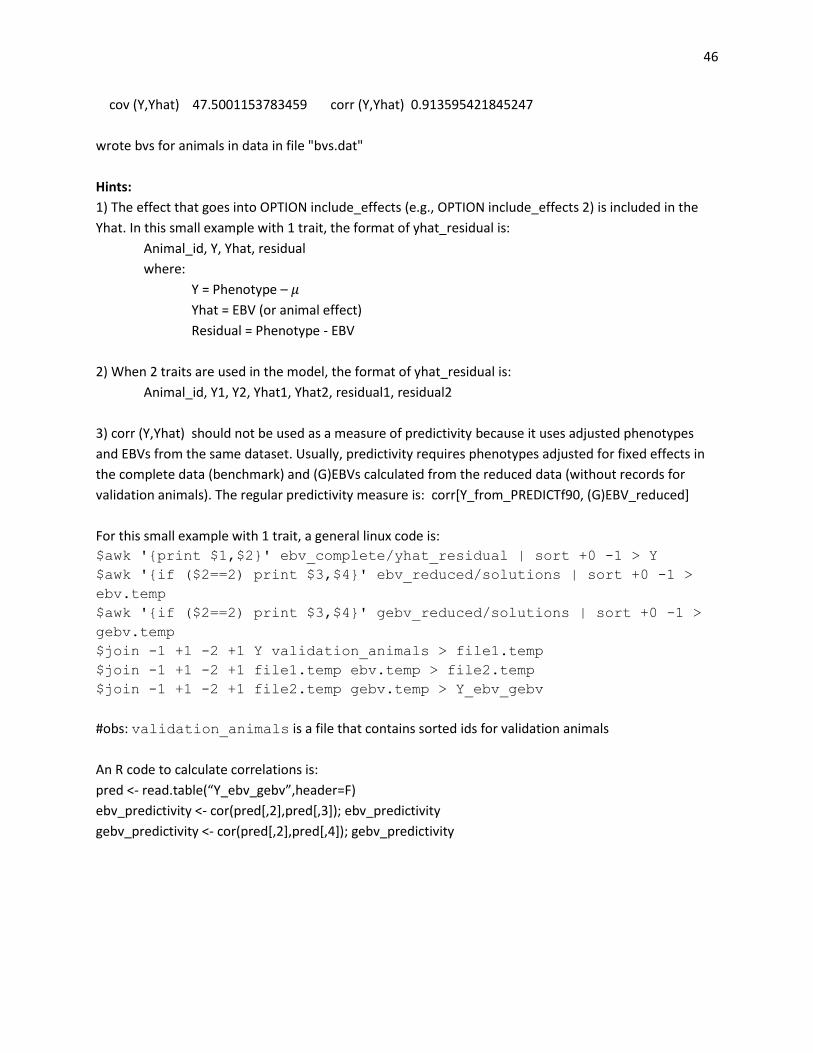
46
cov (Y,Yhat) 47.5001153783459 corr (Y,Yhat) 0.913595421845247
wrote bvs for animals in data in file "bvs.dat"
Hints:
1) The effect that goes into OPTION include_effects (e.g., OPTION include_effects 2) is included in the
Yhat. In this small example with 1 trait, the format of yhat_residual is:
Animal_id, Y, Yhat, residual
where:
Y = Phenotype – 𝜇
Yhat = EBV (or animal effect)
Residual = Phenotype - EBV
2) When 2 traits are used in the model, the format of yhat_residual is:
Animal_id, Y1, Y2, Yhat1, Yhat2, residual1, residual2
3) corr (Y,Yhat) should not be used as a measure of predictivity because it uses adjusted phenotypes
and EBVs from the same dataset. Usually, predictivity requires phenotypes adjusted for fixed effects in
the complete data (benchmark) and (G)EBVs calculated from the reduced data (without records for
validation animals). The regular predictivity measure is: corr[Y_from_PREDICTf90, (G)EBV_reduced]
For this small example with 1 trait, a general linux code is:
$awk '{print $1,$2}' ebv_complete/yhat_residual | sort +0 -1 > Y
$awk '{if ($2==2) print $3,$4}' ebv_reduced/solutions | sort +0 -1 >
ebv.temp
$awk '{if ($2==2) print $3,$4}' gebv_reduced/solutions | sort +0 -1 >
gebv.temp
$join -1 +1 -2 +1 Y validation_animals > file1.temp
$join -1 +1 -2 +1 file1.temp ebv.temp > file2.temp
$join -1 +1 -2 +1 file2.temp gebv.temp > Y_ebv_gebv
#obs: validation_animals is a file that contains sorted ids for validation animals
An R code to calculate correlations is:
pred <- read.table(“Y_ebv_gebv”,header=F)
ebv_predictivity <- cor(pred[,2],pred[,3]); ebv_predictivity
gebv_predictivity <- cor(pred[,2],pred[,4]); gebv_predictivity

47
Examples for parameter files
Sire model without A matrix DATAFILE
test.dat
NUMBER_OF_TRAITS
1
NUMBER_OF_EFFECTS
2
OBSERVATION(S)
3
WEIGHT(S)
EFFECTS: POSITIONS_IN_DATAFILE NUMBER_OF_LEVELS TYPE_OF_EFFECT [EFFECT NESTED]
1 2 cross
2 3 cross
RANDOM_RESIDUAL VALUES
10
RANDOM_GROUP
2
RANDOM_TYPE
diagonal
FILE
(CO)VARIANCES
1
Sire model with A matrix DATAFILE
test.dat
NUMBER_OF_TRAITS
1
NUMBER_OF_EFFECTS
2
OBSERVATION(S)
3
WEIGHT(S)
EFFECTS: POSITIONS_IN_DATAFILE NUMBER_OF_LEVELS TYPE_OF_EFFECT [EFFECT NESTED]
1 2 cross
2 3 cross
RANDOM_RESIDUAL VALUES
10
RANDOM_GROUP
2
RANDOM_TYPE
add_sire
FILE
sire.ped
(CO)VARIANCES
1
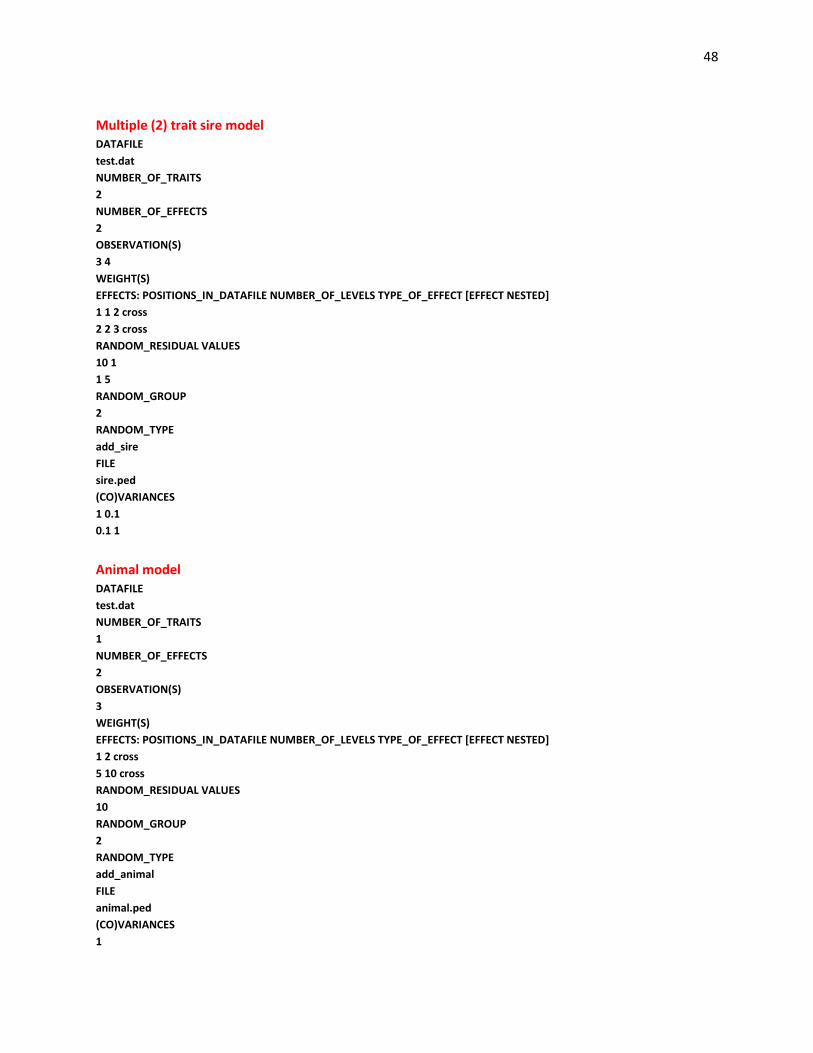
48
Multiple (2) trait sire model DATAFILE
test.dat
NUMBER_OF_TRAITS
2
NUMBER_OF_EFFECTS
2
OBSERVATION(S)
3 4
WEIGHT(S)
EFFECTS: POSITIONS_IN_DATAFILE NUMBER_OF_LEVELS TYPE_OF_EFFECT [EFFECT NESTED]
1 1 2 cross
2 2 3 cross
RANDOM_RESIDUAL VALUES
10 1
1 5
RANDOM_GROUP
2
RANDOM_TYPE
add_sire
FILE
sire.ped
(CO)VARIANCES
1 0.1
0.1 1
Animal model DATAFILE
test.dat
NUMBER_OF_TRAITS
1
NUMBER_OF_EFFECTS
2
OBSERVATION(S)
3
WEIGHT(S)
EFFECTS: POSITIONS_IN_DATAFILE NUMBER_OF_LEVELS TYPE_OF_EFFECT [EFFECT NESTED]
1 2 cross
5 10 cross
RANDOM_RESIDUAL VALUES
10
RANDOM_GROUP
2
RANDOM_TYPE
add_animal
FILE
animal.ped
(CO)VARIANCES
1

49
Multiple trait animal model
# Example 1: 2 trait animal model DATAFILE
test.dat
NUMBER_OF_TRAITS
2
NUMBER_OF_EFFECTS
2
OBSERVATION(S)
3 4
WEIGHT(S)
EFFECTS: POSITIONS_IN_DATAFILE NUMBER_OF_LEVELS TYPE_OF_EFFECT [EFFECT NESTED]
1 1 2 cross
5 5 10 cross
RANDOM_RESIDUAL VALUES
10 1
1 5
RANDOM_GROUP
2
RANDOM_TYPE
add_animal
FILE
animal.ped
(CO)VARIANCES
1 0.1
0.1 1
# Example 2: different model for each trait DATAFILE
test.dat
NUMBER_OF_TRAITS
2
NUMBER_OF_EFFECTS
3
OBSERVATION(S)
3 4
WEIGHT(S)
EFFECTS: POSITIONS_IN_DATAFILE NUMBER_OF_LEVELS TYPE_OF_EFFECT [EFFECT NESTED]
1 2 2 cross
5 5 10 cross
6 7 30 cross
RANDOM_RESIDUAL VALUES
10 1
1 5
RANDOM_GROUP
2
RANDOM_TYPE
add_animal
FILE

50
animal.ped
(CO)VARIANCES
1 0.1
0.1 1
RANDOM_GROUP
3
RANDOM_TYPE
diagonal
FILE
(CO)VARIANCES
1 0
0 1
Animal model with UPG DATAFILE
test.dat
NUMBER_OF_TRAITS
2
NUMBER_OF_EFFECTS
2
OBSERVATION(S)
3 4
WEIGHT(S)
EFFECTS: POSITIONS_IN_DATAFILE NUMBER_OF_LEVELS TYPE_OF_EFFECT [EFFECT NESTED]
1 1 2 cross
5 5 13 cross
RANDOM_RESIDUAL VALUES
10 1
1 5
RANDOM_GROUP
2
RANDOM_TYPE
add_an_upg
FILE
animal.ped
(CO)VARIANCES
1 0.1
0.1 1
Animal model with inbreeding DATAFILE
test.dat
NUMBER_OF_TRAITS
2
NUMBER_OF_EFFECTS
2
OBSERVATION(S)
3 4
WEIGHT(S)

51
EFFECTS: POSITIONS_IN_DATAFILE NUMBER_OF_LEVELS TYPE_OF_EFFECT [EFFECT NESTED]
1 1 2 cross
5 5 13 cross
RANDOM_RESIDUAL VALUES
10 1
1 5
RANDOM_GROUP
2
RANDOM_TYPE
add_an_upginb
FILE
animal.ped
(CO)VARIANCES
1 0.1
0.1 1
Repeatability model 1 DATAFILE
test.dat
NUMBER_OF_TRAITS
1
NUMBER_OF_EFFECTS
3
OBSERVATION(S)
3
WEIGHT(S)
EFFECTS: POSITIONS_IN_DATAFILE NUMBER_OF_LEVELS TYPE_OF_EFFECT [EFFECT NESTED]
1 2 cross
5 5 cross
5 10 cross
RANDOM_RESIDUAL VALUES
10
RANDOM_GROUP
2
RANDOM_TYPE
add_animal
FILE
animal.ped
(CO)VARIANCES
1
RANDOM_GROUP
3
RANDOM_TYPE
diagonal
FILE
(CO)VARIANCES
1
Repeatability model 2

52
DATAFILE
test.dat
NUMBER_OF_TRAITS
2
NUMBER_OF_EFFECTS
3
OBSERVATION(S)
3 4
WEIGHT(S)
EFFECTS: POSITIONS_IN_DATAFILE NUMBER_OF_LEVELS TYPE_OF_EFFECT [EFFECT NESTED]
1 1 2 cross
5 5 5 cross
5 5 10 cross
RANDOM_RESIDUAL VALUES
10 1
1 5
RANDOM_GROUP
2
RANDOM_TYPE
add_animal
FILE
animal.ped
(CO)VARIANCES
1 0.1
0.1 1
RANDOM_GROUP
3
RANDOM_TYPE
diagonal
FILE
(CO)VARIANCES
1 0.1
0.1 1
Maternal effect model DATAFILE
maternal.dat
NUMBER_OF_TRAITS
1
NUMBER_OF_EFFECTS
4
OBSERVATION(S)
4
WEIGHT(S)
EFFECTS: POSITIONS_IN_DATAFILE NUMBER_OF_LEVELS TYPE_OF_EFFECT [EFFECT NESTED]
3 946 cross
1 22473 cross
2 22473 cross
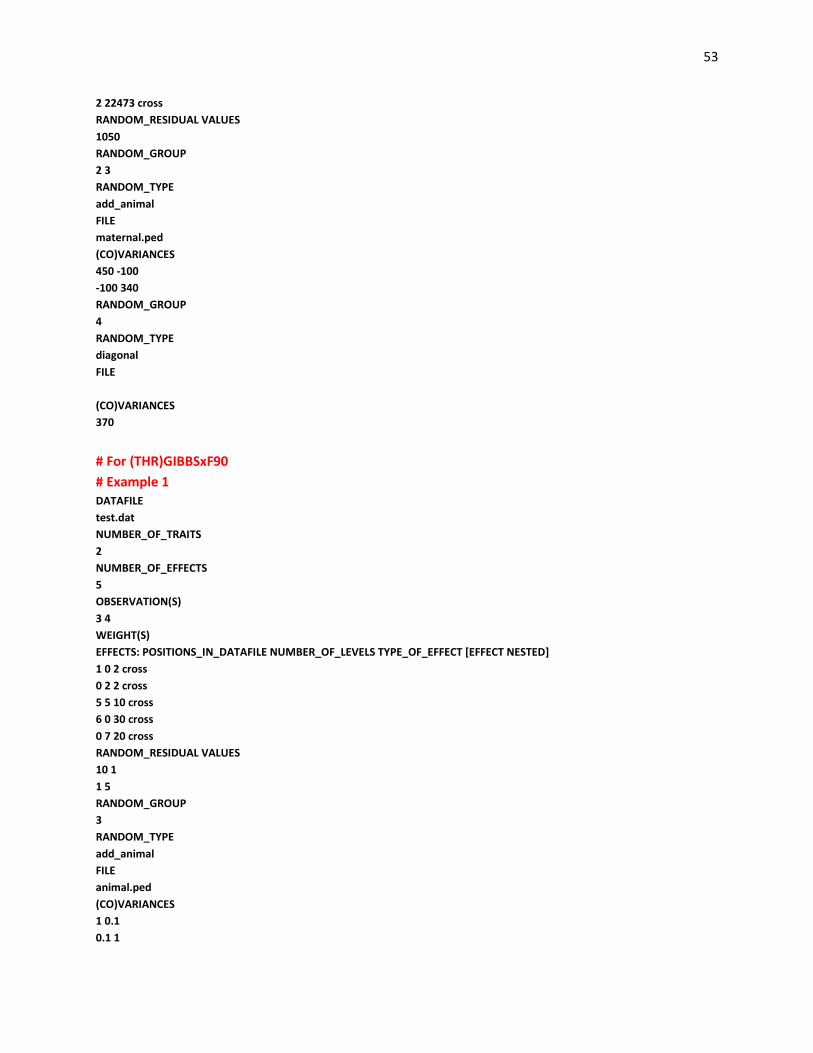
53
2 22473 cross
RANDOM_RESIDUAL VALUES
1050
RANDOM_GROUP
2 3
RANDOM_TYPE
add_animal
FILE
maternal.ped
(CO)VARIANCES
450 -100
-100 340
RANDOM_GROUP
4
RANDOM_TYPE
diagonal
FILE
(CO)VARIANCES
370
# For (THR)GIBBSxF90
# Example 1 DATAFILE
test.dat
NUMBER_OF_TRAITS
2
NUMBER_OF_EFFECTS
5
OBSERVATION(S)
3 4
WEIGHT(S)
EFFECTS: POSITIONS_IN_DATAFILE NUMBER_OF_LEVELS TYPE_OF_EFFECT [EFFECT NESTED]
1 0 2 cross
0 2 2 cross
5 5 10 cross
6 0 30 cross
0 7 20 cross
RANDOM_RESIDUAL VALUES
10 1
1 5
RANDOM_GROUP
3
RANDOM_TYPE
add_animal
FILE
animal.ped
(CO)VARIANCES
1 0.1
0.1 1

54
RANDOM_GROUP
4
RANDOM_TYPE
diagonal
FILE
(CO)VARIANCES
1 0
0 0
RANDOM_GROUP
5
RANDOM_TYPE
diagonal
FILE
(CO)VARIANCES
0 0
0 1
# Example 2 DATAFILE
test.dat
NUMBER_OF_TRAITS
2
NUMBER_OF_EFFECTS
5
OBSERVATION(S)
3 4
WEIGHT(S)
EFFECTS: POSITIONS_IN_DATAFILE NUMBER_OF_LEVELS TYPE_OF_EFFECT [EFFECT NESTED]
1 0 2 cross
0 2 2 cross
5 5 10 cross
6 0 30 cross
0 7 30 cross
RANDOM_RESIDUAL VALUES
10 1
1 5
RANDOM_GROUP
3
RANDOM_TYPE
add_animal
FILE
animal.ped
(CO)VARIANCES
1 0.1
0.1 1
RANDOM_GROUP
4 5
RANDOM_TYPE

55
diagonal
FILE
(CO)VARIANCES
1 0 0 0
0 0 0 0
0 0 0 0
0 0 0 1
# Dominance model DATAFILE
dom.dat
NUMBER_OF_TRAITS
1
NUMBER_OF_EFFECTS
4
OBSERVATION(S)
3
WEIGHT(S)
EFFECTS: POSITIONS_IN_DATAFILE NUMBER_OF_LEVELS TYPE_OF_EFFECT [EFFECT NESTED]
1 1 cross
4 1 cov
2 30001 cross
5 10412 cross
RANDOM_RESIDUAL VALUES
100
RANDOM_GROUP
3
RANDOM_TYPE
add_an_upginb
FILE
add.ped
(CO)VARIANCES
10
RANDOM_GROUP
4
RANDOM_TYPE
par_dom
FILE
dom.ped
(CO)VARIANCES
2
Random regression model
# Example 1 DATAFILE
data_score
NUMBER_OF_TRAITS
1

56
NUMBER_OF_EFFECTS
10
OBSERVATION(S)
9
WEIGHT(S)
EFFECTS: POSITIONS_IN_DATAFILE NUMBER_OF_LEVELS TYPE_OF_EFFECT [EFFECT NESTED]
1 788 cross
2 32 cross
5 1 cov
6 1 cov
3 15097 cross
5 15097 cov 3
6 15097 cov 3
3 81883 cross
5 81883 cov 3
6 81883 cov 3
RANDOM_RESIDUAL VALUES
100
RANDOM_GROUP
5 6 7
RANDOM_TYPE
diagonal
FILE
(CO)VARIANCES
100 1 1
1 10 1
1 1 10
RANDOM_GROUP
8 9 10
RANDOM_TYPE
add_an_upg
FILE
ped_score
(CO)VARIANCES
100 1 1
1 10 1
1 1 10
# Example 2 DATAFILE
test.dat1
NUMBER_OF_TRAITS
2
NUMBER_OF_EFFECTS
9
OBSERVATION(S)
3 4
WEIGHT(S)

57
EFFECTS: POSITIONS_IN_DATAFILE NUMBER_OF_LEVELS TYPE_OF_EFFECT [EFFECT NESTED]
1 1 2 cross
6 6 1 cov
7 7 1 cov
2 2 5 cross
6 6 5 cov 2 2
7 7 5 cov 2 2
2 2 10 cross
6 6 10 cov 2 2
7 7 10 cov 2 2
RANDOM_RESIDUAL VALUES
10 1
1 5
RANDOM_GROUP
4 5 6
RANDOM_TYPE
diagonal
FILE
(CO)VARIANCES
1 0.1 0.1 0.1 0.1 0.1
0.1 1 0.1 0.1 0.1 0.1
0.1 0.1 1 0.1 0.1 0.1
0.1 0.1 0.1 1 0.1 0.1
0.1 0.1 0.1 0.1 1 0.1
0.1 0.1 0.1 0.1 0.1 1
RANDOM_GROUP
7 8 9
RANDOM_TYPE
add_animal
FILE
animal.ped
(CO)VARIANCES
1 0.1 0.1 0.1 0.1 0.1
0.1 1 0.1 0.1 0.1 0.1
0.1 0.1 1 0.1 0.1 0.1
0.1 0.1 0.1 1 0.1 0.1
0.1 0.1 0.1 0.1 1 0.1
0.1 0.1 0.1 0.1 0.1 1
# Example 3 DATAFILE
test.dat2
NUMBER_OF_TRAITS
2
NUMBER_OF_EFFECTS
10
OBSERVATION(S)
3 4
WEIGHT(S)
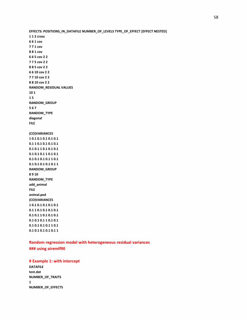
58
EFFECTS: POSITIONS_IN_DATAFILE NUMBER_OF_LEVELS TYPE_OF_EFFECT [EFFECT NESTED]
1 1 2 cross
6 6 1 cov
7 7 1 cov
8 8 1 cov
6 6 5 cov 2 2
7 7 5 cov 2 2
8 8 5 cov 2 2
6 6 10 cov 2 2
7 7 10 cov 2 2
8 8 10 cov 2 2
RANDOM_RESIDUAL VALUES
10 1
1 5
RANDOM_GROUP
5 6 7
RANDOM_TYPE
diagonal
FILE
(CO)VARIANCES
1 0.1 0.1 0.1 0.1 0.1
0.1 1 0.1 0.1 0.1 0.1
0.1 0.1 1 0.1 0.1 0.1
0.1 0.1 0.1 1 0.1 0.1
0.1 0.1 0.1 0.1 1 0.1
0.1 0.1 0.1 0.1 0.1 1
RANDOM_GROUP
8 9 10
RANDOM_TYPE
add_animal
FILE
animal.ped
(CO)VARIANCES
1 0.1 0.1 0.1 0.1 0.1
0.1 1 0.1 0.1 0.1 0.1
0.1 0.1 1 0.1 0.1 0.1
0.1 0.1 0.1 1 0.1 0.1
0.1 0.1 0.1 0.1 1 0.1
0.1 0.1 0.1 0.1 0.1 1
Random regression model with heterogeneous residual variances
### using airemlf90
# Example 1: with intercept DATAFILE
test.dat
NUMBER_OF_TRAITS
1
NUMBER_OF_EFFECTS

59
9
OBSERVATION(S)
3
WEIGHT(S)
EFFECTS: POSITIONS_IN_DATAFILE NUMBER_OF_LEVELS TYPE_OF_EFFECT [EFFECT NESTED]
1 2 cross
6 1 cov
7 1 cov
5 5 cross
6 5 cov 5
7 5 cov 5
5 10 cross
6 10 cov 5
7 10 cov 5
RANDOM_RESIDUAL VALUES
10
RANDOM_GROUP
4 5 6
RANDOM_TYPE
diagonal
FILE
(CO)VARIANCES
1 0.1 0.1
0.1 1 0.1
0.1 0.1 1
RANDOM_GROUP
7 8 9
RANDOM_TYPE
add_animal
FILE
animal.ped
(CO)VARIANCES
1 0.1 0.1
0.1 1 0.1
0.1 0.1 1
OPTION hetres_pos 6 7
OPTION hetres_pol 4.0 1.0 0.1
# Example 2: with no intercept DATAFILE
test.dat
NUMBER_OF_TRAITS
1
NUMBER_OF_EFFECTS
7
OBSERVATION(S)
3
WEIGHT(S)
EFFECTS: POSITIONS_IN_DATAFILE NUMBER_OF_LEVELS TYPE_OF_EFFECT [EFFECT NESTED]

60
1 2 cross
6 1 cov
7 1 cov
6 5 cov 5
7 5 cov 5
6 10 cov 5
7 10 cov 5
RANDOM_RESIDUAL VALUES
10
RANDOM_GROUP
4 5
RANDOM_TYPE
diagonal
FILE
(CO)VARIANCES
1 0.1
0.1 1
RANDOM_GROUP
6 7
RANDOM_TYPE
add_animal
FILE
animal.ped
(CO)VARIANCES
1 0.1
0.1 1
OPTION hetres_pos 6 7
OPTION hetres_pol 1.0 0.1
### using GIBBS3F90 DATAFILE
test.dat
NUMBER_OF_TRAITS
1
NUMBER_OF_EFFECTS
9
OBSERVATION(S)
3
WEIGHT(S)
EFFECTS: POSITIONS_IN_DATAFILE NUMBER_OF_LEVELS TYPE_OF_EFFECT [EFFECT NESTED]
1 2 cross
6 1 cov
7 1 cov
5 5 cross
6 5 cov 5
7 5 cov 5
5 10 cross
6 10 cov 5
7 10 cov 5

61
RANDOM_RESIDUAL VALUES
10
RANDOM_GROUP
4 5 6
RANDOM_TYPE
diagonal
FILE
(CO)VARIANCES
1 0.1 0.1
0.1 1 0.1
0.1 0.1 1
RANDOM_GROUP
7 8 9
RANDOM_TYPE
add_animal
FILE
animal.ped
(CO)VARIANCES
1 0.1 0.1
0.1 1 0.1
0.1 0.1 1
OPTION hetres_int 8 5
Competitive model DATAFILE
competition.dat
NUMBER_OF_TRAITS
1
NUMBER_OF_EFFECTS
19
OBSERVATION(S)
24
WEIGHT(S)
EFFECTS: POSITIONS_IN_DATAFILE NUMBER_OF_LEVELS TYPE_OF_EFFECT[EFFECT NESTED]
2 88 cross
3 362 cross
21 2409 cross
4 8004 cross
22 0 cov 5
22 0 cov 6
22 0 cov 7
22 0 cov 8
22 0 cov 9
22 0 cov 10
22 0 cov 11
22 0 cov 12
22 0 cov 13
22 0 cov 14

62
22 0 cov 15
22 0 cov 16
22 0 cov 17
22 0 cov 18
22 8004 cov 19
RANDOM_RESIDUAL VALUES
1225.8
RANDOM_GROUP
4 5
RANDOM_TYPE
add_animal
FILE
renadd04.ped
(CO)VARIANCES
267.03 25.313
25.313 104.44
RANDOM_GROUP
2
RANDOM_TYPE
diagonal
FILE
(CO)VARIANCES
89.187
RANDOM_GROUP
3
RANDOM_TYPE
diagonal
FILE
(CO)VARIANCES
167.34
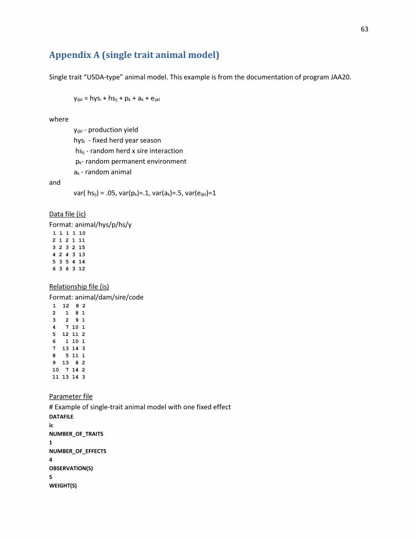
63
Appendix A (single trait animal model)
Single trait “USDA-type” animal model. This example is from the documentation of program JAA20.
yijkl = hysi + hsij + pk + ak + eijkl
where
yijkl - production yield
hysi - fixed herd year season
hsij - random herd x sire interaction
pk- random permanent environment
ak - random animal
and
var( hsij) = .05, var(pk)=.1, var(ak)=.5, var(eijkl)=1
Data file (ic)
Format: animal/hys/p/hs/y 1 1 1 1 10
2 1 2 1 11
3 2 3 2 15
4 2 4 3 13
5 3 5 4 14
6 3 6 3 12
Relationship file (is)
Format: animal/dam/sire/code 1 12 8 2
2 1 8 1
3 2 9 1
4 7 10 1
5 12 11 2
6 1 10 1
7 13 14 3
8 5 11 1
9 13 8 2
10 7 14 2
11 13 14 3
Parameter file
# Example of single-trait animal model with one fixed effect DATAFILE
ic
NUMBER_OF_TRAITS
1
NUMBER_OF_EFFECTS
4
OBSERVATION(S)
5
WEIGHT(S)

64
EFFECTS: POSITIONS_IN_DATAFILE NUMBER_OF_LEVELS TYPE_OF_EFFECT [EFFECT NESTED]
2 3 cross
3 6 cross
4 4 cross
1 14 cross
RANDOM_RESIDUAL VALUES
1
RANDOM_GROUP
2
RANDOM_TYPE
diagonal
FILE
(CO)VARIANCES
.1
RANDOM_GROUP
3
RANDOM_TYPE
diagonal
FILE
(CO)VARIANCES
.05
RANDOM_GROUP
4
RANDOM_TYPE
add_an_upg
FILE
is
(CO)VARIANCES
.5
Execution name of parameter file?exiap
BLUPF90 1.00
Parameter file: exiap
Data file: ic
Number of Traits 1
Number of Effects 4
Position of Observations 5
Position of Weight (1) 0
Value of Missing Trait/Observation 0
EFFECTS
# type position (2) levels [positions for nested]
1 cross-classified 2 3
2 cross-classified 3 6
3 cross-classified 4 4
4 cross-classified 1 14

65
Residual (co)variance Matrix
1.000
Random Effect 2
Type of Random Effect: diagonal
trait effect (CO)VARIANCES
1 2 0.100
Random Effect 3
Type of Random Effect: diagonal
trait effect (CO)VARIANCES
1 3 0.050
Random Effect 4
Type of Random Effect: additive animal
Pedigree File: is
trait effect (CO)VARIANCES
1 4 0.500
REMARKS
(1) Weight position 0 means no weights utilized
(2) Effect positions of 0 for some effects and traits means that such
effects are missing for specified traits
Data record length = 5
original G
0.10
inverted G
10.00
original G
0.05
inverted G
20.00
original G
0.50
inverted G
2.00
solutions stored in file: "solutions"
trait/effect level solution
1 1 1 11.8589
1 1 2 13.7539
1 1 3 14.7086
1 2 1 -0.0088
1 2 2 0.0088
1 2 3 -0.0159
1 2 4 0.0159
1 2 5 0.0321
1 2 6 -0.0321
1 3 1 0.0000
1 3 2 -0.0079
1 3 3 -0.0081
1 3 4 0.0161
1 4 1 -1.7627
1 4 2 -0.9553
1 4 3 1.4288
1 4 4 -0.9206
1 4 5 -1.0781
1 4 6 -2.3474
1 4 7 0.8511
1 4 8 -0.1521
1 4 9 3.8926
1 4 10 -2.7717

66
1 4 11 0.8528
1 4 12 -3.1911
1 4 13 7.9976
1 4 14 -6.3340

67
Appendix B (multiple trait sire model)
Example of multiple trait sire model (from L.R. Schaeffer notes of 1985).
Models
Trait 1: y1i=hi+s1j+e1ijk
Trait 2: y2i=μ+s2j+e2jk
where
h - fixed herd
s - random sire
and
var(s)=A[8 6; 6 17], var(e)=I[10 10; 10 20]
Data file (lrsdat)
Format: h/μ/s/y1/y2 1 0 1 3.4 0
2 0 2 1.3 0
1 1 3 .8 50.3
2 1 4 4.5 52.6
0 1 5 0 55.0
Pedigree file (lrsrel)
Format: bull/sire/MGS 1 3 0
2 0 5
3 0 0
4 0 0
5 0 0
Parameter file (lrsex) # Example of two trait sire model with unequal models
DATAFILE
lrsdat
NUMBER_OF_TRAITS
2
NUMBER_OF_EFFECTS
2
OBSERVATION(S)
4 5
WEIGHT(S)
EFFECTS: POSITIONS_IN_DATAFILE NUMBER_OF_LEVELS TYPE_OF_EFFECT [EFFECT NESTED]
1 2 2 cross
3 3 5 cross
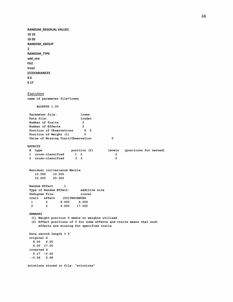
68
RANDOM_RESIDUAL VALUES
10 10
10 20
RANDOM_GROUP
2
RANDOM_TYPE
add_sire
FILE
lrsrel
(CO)VARIANCES
8 6
6 17
Execution name of parameter file?lrsex
BLUPF90 1.00
Parameter file: lrsex
Data file: lrsdat
Number of Traits 2
Number of Effects 2
Position of Observations 4 5
Position of Weight (1) 0
Value of Missing Trait/Observation 0
EFFECTS
# type position (2) levels [positions for nested]
1 cross-classified 1 2 2
2 cross-classified 3 3 5
Residual (co)variance Matrix
10.000 10.000
10.000 20.000
Random Effect 1
Type of Random Effect: additive sire
Pedigree File: lrsrel
trait effect (CO)VARIANCES
1 2 8.000 6.000
2 2 6.000 17.000
REMARKS
(1) Weight position 0 means no weights utilized
(2) Effect positions of 0 for some effects and traits means that such
effects are missing for specified traits
Data record length = 5
original G
8.00 6.00
6.00 17.00
inverted G
0.17 -0.06
-0.06 0.08
solutions stored in file: "solutions"

69
trait/effect level solution
1 1 1 2.3877
2 1 1 52.4449
1 1 2 3.2180
2 1 2 0.0000
1 2 1 0.2243
2 2 1 -0.0210
1 2 2 -0.8217
2 2 2 -0.3866
1 2 3 -0.4969
2 2 3 -0.7512
1 2 4 0.6178
2 2 4 -0.0769
1 2 5 0.2217
2 2 5 1.0851

70
Appendix C (test-day model)
This test-day model example comes from the paper of Schaeffer and Dekkers (WCGALP94 18:443)
Model
yijkl = hi + β1X1j + β2X2j + ak + γ1kX1j + γ2kX2j +eijkl
where
yijkl - yield of test day
hi - test day effect
X1j - days in milk
X2j - log(days in milk)
β1, β2 - fixed regressions
ak - random animal
γ1k, γ2k - random regressions for each animal
and
var(eijkl) = 1; var(ak, γ1k, γ2k ) = [ 2.25 4 -.7; 4 1375 12; -.7 12 94]-1
Data file (lrsrrdat)
Format: h/a/X1/X2/y 1 1 73 1.42985 26
1 2 34 2.19395 29
1 3 8 3.64087 37
2 1 123 0.908127 23
2 2 84 1.28949 18
2 3 58 1.65987 25
2 4 5 4.11087 44
3 1 178 0.538528 21
3 2 139 0.785838 8
3 3 113 0.992924 19
3 4 60 1.62597 29
4 2 184 0.505376 1
4 3 158 0.657717 15
4 4 105 1.06635 22
4 5 14 3.08125 35
5 3 218 0.335817 11
5 4 165 0.614366 14
5 5 74 1.41625 23
5 6 31 2.28632 28
6 3 268 0.129325 7
6 4 215 0.349674 8
6 5 124 0.90003 17
6 6 81 1.32586 22
Relationship file (lrsrrrel)
Format: animal/sire/dam 1 9 7
2 10 8
3 9 2
4 10 8
5 11 7
6 11 1

71
7 0 0
8 0 0
9 0 0
10 0 0
11 0 0
Parameter file (exlrsrr) # Example of single-trait random-regression model
DATAFILE
lrsrrdat
NUMBER_OF_TRAITS
1
NUMBER_OF_EFFECTS
6
OBSERVATION(S)
5
WEIGHT(S)
EFFECTS: POSITIONS_IN_DATAFILE NUMBER_OF_LEVELS TYPE_OF_EFFECT [EFFECT NESTED]
1 6 cross
3 1 cov
4 1 cov
2 11 cross
3 11 cov 2
4 11 cov 2
RANDOM_RESIDUAL VALUES
1
RANDOM_GROUP
4 5 6
RANDOM_TYPE
add_animal
FILE
lrsrrrel
(CO)VARIANCES
.447906 -0.001334 0.003506
-0.001334 0.000732 -0.000103
0.003506 -0.000103 .010678
Execution name of parameter file?exlrsrr
BLUPF90 1.00
Parameter file: exlrsrr
Data file: lrsrrdat
Number of Traits 1
Number of Effects 6
Position of Observations 5
Position of Weight (1) 0
Value of Missing Trait/Observation 0
EFFECTS
# type position (2) levels [positions for nested]
1 cross-classified 1 6
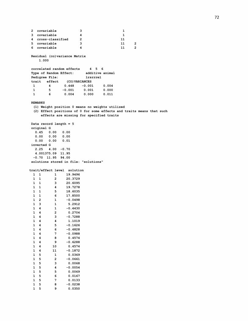
72
2 covariable 3 1
3 covariable 4 1
4 cross-classified 2 11
5 covariable 3 11 2
6 covariable 4 11 2
Residual (co)variance Matrix
1.000
correlated random effects 4 5 6
Type of Random Effect: additive animal
Pedigree File: lrsrrrel
trait effect (CO)VARIANCES
1 4 0.448 -0.001 0.004
1 5 -0.001 0.001 0.000
1 6 0.004 0.000 0.011
REMARKS
(1) Weight position 0 means no weights utilized
(2) Effect positions of 0 for some effects and traits means that such
effects are missing for specified traits
Data record length = 5
original G
0.45 0.00 0.00
0.00 0.00 0.00
0.00 0.00 0.01
inverted G
2.25 4.00 -0.70
4.001375.09 11.95
-0.70 11.95 94.00
solutions stored in file: "solutions"
trait/effect level solution
1 1 1 19.9496
1 1 2 20.3729
1 1 3 20.6095
1 1 4 19.7278
1 1 5 18.6035
1 1 6 17.8500
1 2 1 -0.0498
1 3 1 5.2912
1 4 1 -0.4430
1 4 2 0.2704
1 4 3 -0.7288
1 4 4 1.1019
1 4 5 -0.1626
1 4 6 -0.4828
1 4 7 -0.0988
1 4 8 0.4574
1 4 9 -0.6288
1 4 10 0.4574
1 4 11 -0.1872
1 5 1 0.0369
1 5 2 -0.0661
1 5 3 0.0068
1 5 4 -0.0054
1 5 5 0.0069
1 5 6 0.0167
1 5 7 0.0133
1 5 8 -0.0238
1 5 9 0.0350

73
1 5 10 -0.0238
1 5 11 -0.0008
1 6 1 -0.0370
1 6 2 0.0325
1 6 3 -0.0479
1 6 4 0.0767
1 6 5 -0.0149
1 6 6 -0.0377
1 6 7 -0.0103
1 6 8 0.0364
1 6 9 -0.0480
1 6 10 0.0364
1 6 11 -0.0145

74
Appendix D (multibreed maternal effect model)
This model was used for studies on multibreed evaluation in beef cattle. It is provided as an example of
a model with maternal effect and different models per trait.
Model (in concise form, with most indices omitted)
y1=cg1 + bt + mbt + a + M + e
y2=cg2 + bt + mbt + a + M + pe + e
y3=cg3 + bt + mbt + a + e
where
y1-3 - birth weight, weaning weight, and gain
cg1-3 - contemporary groups separate for each trait
br - breed type
mbt - maternal breed type
a - additive effect
m - maternal effect
pe - permanent environmental effect of the dam
Data file (data.out)
Format:
1. contemporary group for trait 1
2. contemporary group for trait 2
3. contemporary group for trait 3
4. animal breed type
5. maternal breed type
6. animal id
7. dam id
8. birth weight
9. weaning weight
10. gain
Relationship file (pedi.outok)
Format:
animal
sire or unknown parent group
dam or unknown parent group
“1 + number of missing parents”
Parameter file (exlrsrr) DATAFILE

75
data.out
NUMBER_OF_TRAITS
3
NUMBER_OF_EFFECTS
6
OBSERVATION(S)
8 9 10
WEIGHT(S)
EFFECTS: POSITIONS_IN_DATAFILE NUMBER_OF_LEVELS TYPE_OF_EFFECT [EFFECT
NESTED]
1 2 3 133085 cross
4 4 4 181 cross
5 5 0 165 cross
6 6 6 1724112 cross
7 7 0 1724112 cross
0 7 0 1724112 cross
RANDOM_RESIDUAL VALUES
26.3 40.7 20.3
40.7 1312.9 141.9
20.3 141.9 1246.3
RANDOM_GROUP
4 5
RANDOM_TYPE
add_an_upg
FILE
pedi.outok
(CO)VARIANCES
22.9 36.3 18.6 -4.6 0.0 0.0
36.6 500.2 110.8 0.0 -91.6 0.0
18.6 110.8 313.0 0.0 0.0 0.0
-4.6 0.0 0.0 10.1 0.0 0.0
0.0 -91.6 0.0 0.0 419.1 0.0
0.0 0.0 0.0 0.0 0.0 0.0
RANDOM_GROUP
2
RANDOM_TYPE
diagonal
FILE
(CO)VARIANCES
0.263 0.0 0.0
0.0 13.129 0.0
0.0 0.0 12.463
RANDOM_GROUP
3
RANDOM_TYPE
diagonal
FILE
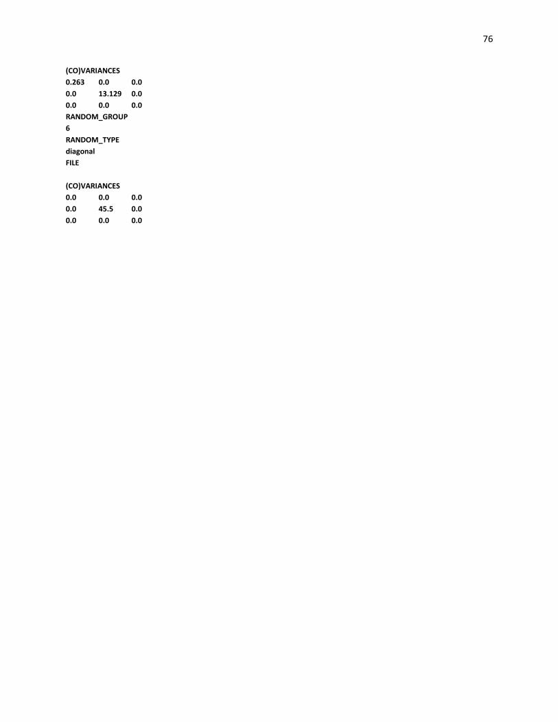
76
(CO)VARIANCES
0.263 0.0 0.0
0.0 13.129 0.0
0.0 0.0 0.0
RANDOM_GROUP
6
RANDOM_TYPE
diagonal
FILE
(CO)VARIANCES
0.0 0.0 0.0
0.0 45.5 0.0
0.0 0.0 0.0
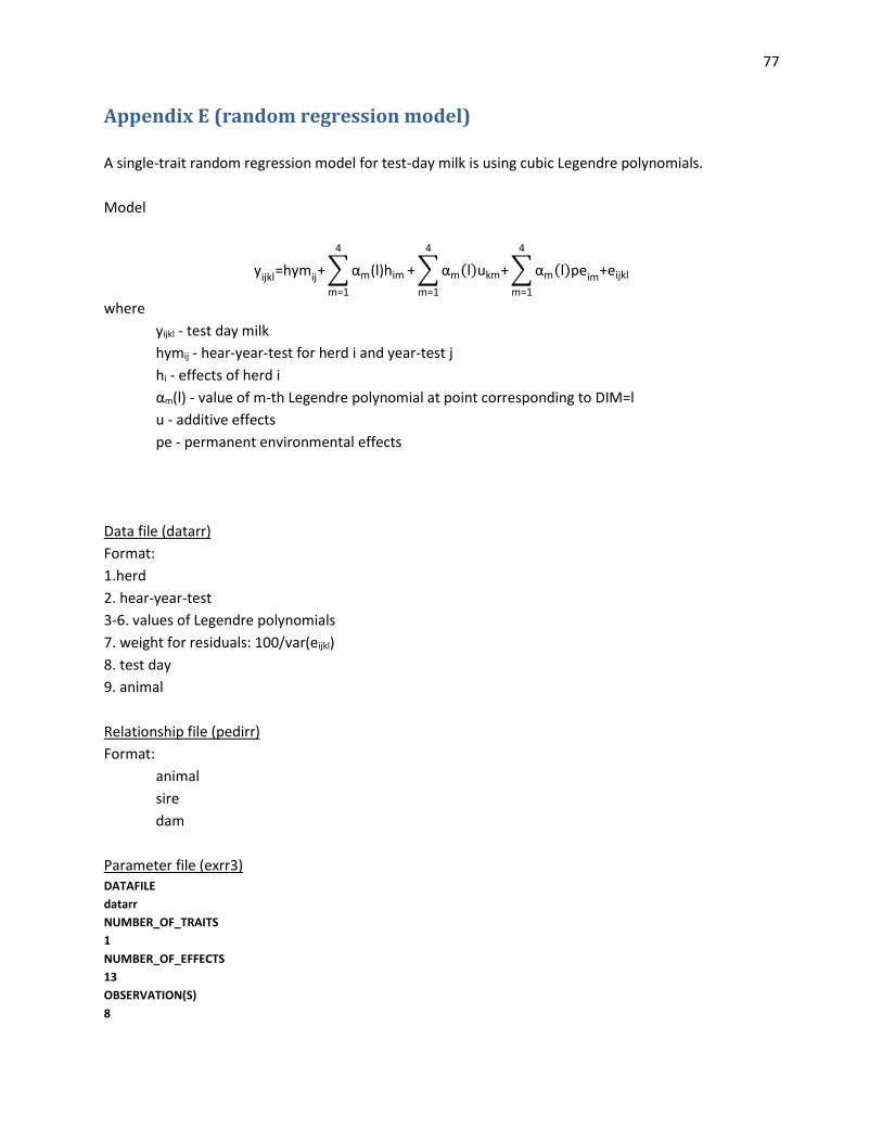
77
Appendix E (random regression model)
A single-trait random regression model for test-day milk is using cubic Legendre polynomials.
Model
yijkl=hymij+∑αm(l)him
4
m=1
+∑αm(l)ukm+∑αm(l)peim+eijkl
4
m=1
4
m=1
where
yijkl - test day milk
hymij - hear-year-test for herd i and year-test j
hi - effects of herd i
αm(l) - value of m-th Legendre polynomial at point corresponding to DIM=l
u - additive effects
pe - permanent environmental effects
Data file (datarr)
Format:
1.herd
2. hear-year-test
3-6. values of Legendre polynomials
7. weight for residuals: 100/var(eijkl)
8. test day
9. animal
Relationship file (pedirr)
Format:
animal
sire
dam
Parameter file (exrr3) DATAFILE
datarr
NUMBER_OF_TRAITS
1
NUMBER_OF_EFFECTS
13
OBSERVATION(S)
8

78
WEIGHT(S)
7
EFFECTS: POSITIONS_IN_DATAFILE NUMBER_OF_LEVELS TYPE_OF_EFFECT
2 3726 cross #herd-year-test
3 84 cov 1 #herd
4 84 cov 1
5 84 cov 1
6 84 cov 1
3 21874 cov 9 #additive
4 21874 cov 9
5 21874 cov 9
6 21874 cov 9
3 21874 cov 9 #pe
4 21874 cov 9
5 21874 cov 9
6 21874 cov 9
RANDOM_RESIDUAL VALUES
100
RANDOM_GROUP
6 7 8 9
RANDOM_TYPE
add_animal
FILE
pedirr
(CO)VARIANCES
(4 x 4 matrix)
RANDOM_GROUP
10 11 12 13
RANDOM_TYPE
diagonal
FILE
(CO)VARIANCES
(4 x 4 matrix)

79
Appendix F (terminal cross model)
A terminal cross model by Fernando et al. and Lo et al.
breed A: ya=cga + ua + ea
breed B: yb=cgb+ ub +eb
cross: yab=cgab+ uaab + ubab +eab
Data file (data_cross)
1. cg A (85 levels)
2. cg B (110 levels)
3. cg crossbred (87 levels)
4. animal - breed A (2400 animals) or parent from breed A
5. animal - breed B (3000 animals) or parent from breed B
6. ya
7. yb
8. yc
Pedigree files: pedig_A for breed A and pedig_B for breed B
Parameter file # Example of a terminal-cross model
DATAFILE
data-cross
NUMBER_OF_TRAITS
3
NUMBER_OF_EFFECTS
3
OBSERVATION(S)
6 7 8
WEIGHT(S)
EFFECTS: POSITIONS_IN_DATAFILE NUMBER_OF_LEVELS TYPE_OF_EFFECT [EFFECT NESTED]
1 2 3 110 cross
4 0 4 2400 cross
0 5 5 3000 cross
RANDOM_RESIDUAL VALUES
100 0 0
0 100 0
0 0 100
RANDOM_GROUP
2
RANDOM_TYPE
add_animal
FILE
pedig_A

80
(CO)VARIANCES
(3 x 3 matrix)
RANDOM_GROUP
3
RANDOM_TYPE
add_animal
FILE
pedig_B
(CO)VARIANCES
(3 x 3 matrix)

81
Appendix G (competitive model)
Example of a competitive model (a la Muir and Schinkel)
y=cg + a +c1 + c2 +..+c5 + e
ci is the effect of the i-th competitor; assumed pen size of up to 6.
Datafile (data_comp)
1. y
2. cg (max 120)
3. animal (max 3000)
4. competitor 1
5. c 2
...
8. c 5
If pen size is less than 6, unused fields set to 0.
Parameter file # Example of a competitive model
DATAFILE
data_comp
NUMBER_OF_TRAITS
1
NUMBER_OF_EFFECTS
7
OBSERVATION(S)
1
WEIGHT(S)
EFFECTS: POSITIONS_IN_DATAFILE NUMBER_OF_LEVELS TYPE_OF_EFFECT [EFFECT NESTED]
2 120 cross
3 3000 cross
4 0 cross
5 0 cross
6 0 cross
7 0 cross
8 3000 cross
RANDOM_RESIDUAL VALUES
50
RANDOM_GROUP
2 3
RANDOM_TYPE
add_animal
FILE
The 2nd effect (position 3 in the data) is additive
direct effect and 3rd to 7th effects (positions 4 to 8
in the data) are competitive effects (animal ID for
competitors).

82
pedig
(CO)VARIANCES
40 -10
-10 10
The covariance matrix contains variance for the
second effect, variance for effects 3 to 7
(accumulated to 7), and covariance between
direct and competitive effects.

83
Appendix H (genomic model) Example of evaluation /variance component estimation using phenotypic, pedigree and genomic information in single-step evaluation Files simulated by Huiyu Wang using program QMSim by Mehdi Sargolzaei & Flavio Schenkel.
DATAFILE phenotypes.txt TRAITS 3 FIELDS_PASSED TO OUTPUT WEIGHT(S) RESIDUAL_VARIANCE 0.9038 EFFECT 1 cross alpha #fixed effect EFFECT 2 cross alpha #animal RANDOM animal FILE pedigree SNP_FILE marker.geno.clean (CO)VARIANCES 0.9951E-01
phenotypes.txt
1 1 4.16 0
1 2 3.47 0
1 3 4.5 0
1 4 4.97 0
1 5 5.98 0
1 6 6.63 0
1 7 3.32 0
1 8 5.85 0
1 9 4.77 0
1 10 4.22 0
pedigree
1 0 0 0
2 0 0 0
3 0 0 0
4 0 0 0
5 0 0 0
Parameter file for renumbering program RENUMF90
Phenotype file
Pedigree file
Phenotypes.txt – phenotype file
Single trait in position 3
Fixed effect in position 1 read as alphanumeric
Random animal effect in position 3
Pedigree file pedigrees
SNP file marker.geno.clean

84
6 0 0 0
7 0 0 0
8 0 0 0
9 0 0 0
10 0 0 0
cut -c1-50 marker.geno.clean|head -10
8002 21101011002012011011010110111111211111210100
8014 21110101111101120221110111111112101112210100
8016 21100101202202021120210121102111202212111101
8018 21110111112201120210200020101022212211111100
8024 21110102201201111220210111102122201221111111
8038 11110000102100120201211121201022112111121111
8041 22210001201201121110210121202111102102121001
8063 20110101202202020212211101101120222012120021
8065 21110101111112111221110101010220212001110012
8083 10111011110010111111110112100111121011010121
RENUMF90 version 1.86
name of parameter file?renum.par
renum.par
datafile:phenotypes.txt
traits: 3
fields passed: 4
R
0.9038
Processing effect 1 of type cross
item_kind=alpha
Processing effect 2 of type cross
item_kind=alpha
pedigree file name "pedigree"
positions of animal, sire, dam, alternate dam and yob 1 2
3 0 0
SNP file name "marker.geno.clean"
all pedigrees to be included
Reading (CO)VARIANCES: 1 x 1
Maximum size of character fields: 20
Maximum size of record (max_string_readline): 800
Maximum number of fields innput file (max_field_readline): 100
hash tables for effects set up
table expanded from 10000 to 20000 records
table expanded from 20000 to 40000 records
read 15800 records
table with 1 elements sorted
added count
Effect group 1 of column 1 with 1 levels
table expanded from 10000 to 10000 records
added count
Effect group 2 of column 1 with 15800 levels
wrote statistics in file "renf90.tables"
Basic statistics for input data (missing value code is 0)
Pos Min Max Mean SD N
3 0.73000 8.8300 4.9793 1.0069 15800
SNP file for the first 50 SNP
Run RENUMF90

85
random effect with SNPs 2
type: animal
file: marker.geno.clean
read SNPs 1500 records
Effect group 2 of column 1 with 15800 levels
random effect 2
type:animal
opened output pedigree file "renadd02.ped"
read 15800 pedigree records
Pedigree checks
Number of animals with records: 15800
Number of animals with genotypes: 1500
Number of animals with records or genotypes: 15800
Number of animals with genotypes and no records 0
Number of parents without records or genotypes: 0
Total number of animals: 15800
Wrote cross reference IDs for SNP file "marker.geno.clean_XrefID"
Wrote parameter file "renf90.par"
Wrote renumbered data "renf90.dat"
renf90.par # BLUPF90 parameter file created by RENF90 DATAFILE
renf90.dat NUMBER_OF_TRAITS 1 NUMBER_OF_EFFECTS 2 OBSERVATION(S) 1 WEIGHT(S) EFFECTS: POSITIONS_IN_DATAFILE NUMBER_OF_LEVELS TYPE_OF_EFFECT[EFFECT NESTED] 2 1 cross 3 15800 cross RANDOM_RESIDUAL VALUES 0.9038 RANDOM_GROUP 2 RANDOM_TYPE add_animal FILE renadd02.ped (CO)VARIANCES 0.9951E-01 OPTION SNP_file marker.geno.clean
renadd02.ped
Parameter file for application programs with renumbered fields
Renumbered pedigree file
renf90.dat – phenotype file
Single trait in position 1
Two effects in model
Fixed effect in position 1 cross-classified with 1 level (μ)
Animal effect in position 3
Second effect (Random Group 2) is additive-animal with
renadd02.ped – pedigree file
SNP file marker.geno.clean

86
1 5742 14705 1 0 2 1 0 0 14670
2 2302 1384 1 0 2 1 0 0 12367
3 4248 15309 1 0 12 1 0 2 9123
4 4241 3492 1 0 2 1 0 0 7455
5 14459 14202 1 0 2 1 0 0 5736
6 1029 1292 1 0 2 1 0 3 5877
7 10876 7596 1 0 2 1 0 0 9638
8 13589 12642 1 0 2 1 0 0 14136
9 7070 11562 1 0 2 1 0 0 6010
10 6449 2448 1 0 2 1 0 0 15498
renf90.dat
4.16 1 5903 0
3.47 1 3628 0
4.5 1 1329 0
4.97 1 14808 0
5.98 1 12481 0
6.63 1 10205 0
3.32 1 7935 0
5.85 1 5639 0
4.77 1 3348 0
4.22 1 1951 0
name of parameter file?renf90.par
* SNP file: marker.geno.clean
* SNP Xref file: marker.geno.clean_XrefID
* Frequency to Center Z=M-p to create G=ZZ'/k (default whichfreq = 2):
2
BLUPF90 1.42
Parameter file: renf90.par
Data file: renf90.dat
Number of Traits 1
Number of Effects 2
Position of Observations 1
Position of Weight (1) 0
Value of Missing Trait/Observation 0
EFFECTS
# type position (2) levels [positions for nested]
1 cross-classified 2 1
2 cross-classified 3 15800
Residual (co)variance Matrix
0.90380
Random Effect(s) 2
Type of Random Effect: additive animal
Pedigree File: renadd02.ped
trait effect (CO)VARIANCES
1 2 0.9951E-01
REMARKS
(1) Weight position 0 means no weights utilized
(2) Effect positions of 0 for some effects and traits means that such
effects are missing for specified traits
Data record length = 3
# equations = 15801
G
0.99510E-01
Renumbered phenotype file
Run BLUPF90
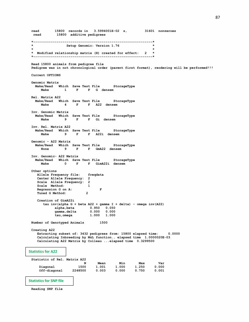
87
read 15800 records in 3.5994001E-02 s, 31601 nonzeroes
read 15800 additive pedigrees
*-------------------------------------------------------------*
* Setup Genomic: Version 1.76 *
* *
* Modified relationship matrix (H) created for effect: 2 *
*-------------------------------------------------------------*
Read 15800 animals from pedigree file
Pedigree was in not chronological order (parent first format), reodering will be performed!!!
Current OPTIONS
Genomic Matrix
Make/Read Which Save Test File StorageType
Make 1 F F G densem
Rel. Matrix A22
Make/Read Which Save Test File StorageType
Make 4 F F A22 densem
Inv. Genomic Matrix
Make/Read Which Save Test File StorageType
Make 9 F F Gi densem
Inv. Rel. Matrix A22
Make/Read Which Save Test File StorageType
Make 9 F F A22i densem
Genomic - A22 Matrix
Make/Read Which Save Test File StorageType
None 9 F F GmA22 densem
Inv. Genomic- A22 Matrix
Make/Read Which Save Test File StorageType
Make 0 F F GimA22i densem
Other options
Allele Frequency file: freqdata
Center Allele Frequency: 2
Scale Allele Frequency: 2
Scale Method: 1
Regression G on A: F
Tuned G Method: 2
Creation of GimA22i
tau inv(alpha G + beta A22 + gamma I + delta) - omega inv(A22)
alpha,beta 0.950 0.050
gamma,delta 0.000 0.000
tau,omega 1.000 1.000
Number of Genotyped Animals 1500
Creating A22
Extracting subset of: 3432 pedigrees from: 15800 elapsed time: 0.0000
Calculating Inbreeding by M&L function.. elapsed time 1.0000020E-03
Calculating A22 Matrix by Colleau ...elapsed time 0.3299500
Statistic of Rel. Matrix A22
N Mean Min Max Var
Diagonal 1500 1.001 1.000 1.250 0.000
Off-diagonal 2248500 0.003 0.000 0.750 0.001
Reading SNP file
Statistics for A22
Statistics for SNP file

88
Column position in file for the first marker: 7
Format to read SNP file: (6x,400000i1)
Number of SNPs : 3000
Number of Genotyped animals: 1500
Reading SNP file elapsed time 0.4639290
Statistics of alleles frequencies in the current population
N: 3000
Mean: 0.501
Min: 0.132
Max: 0.890
Var: 0.014
Quality Control - Check call rate for animals
Quality Control - Check Parent-Progeny Mendelian conflicts
Total animals: 15800 - Genotyped animals: 1500
Number of Individual - Sire pairs: 470
Number of Individual - Dams pairs: 256
Number of Individual - Sire - Dam trios: 152
Checking SNPs for Mendelian conflicts
Total number of parent-progeny evaluations: 726
Number of SNPs with Mendelian conflicts: 0
Checking Animals for Mendelian conflicts
Statistics of alleles frequencies in the current population after
Quality Control (MAF, monomorphic, call rate)
N: 3000
Mean: 0.501
Min: 0.132
Max: 0.890
Var: 0.014
Locus Freq 0-2p 1-2p 2-2p
1 0.751333 -1.502667 -0.502667 0.497333
2 0.382333 -0.764667 0.235333 1.235333
3 0.568667 -1.137333 -0.137333 0.862667
4 0.680000 -1.360000 -0.360000 0.640000
5 0.184333 -0.368667 0.631333 1.631333
6 0.298333 -0.596667 0.403333 1.403333
7 0.392000 -0.784000 0.216000 1.216000
8 0.379667 -0.759333 0.240667 1.240667
9 0.596667 -1.193333 -0.193333 0.806667
10 0.352333 -0.704667 0.295333 1.295333
Genotypes missings (%): 0.0000000E+00
Average denom. (scale): 1415.90178466665
Center Matrix elapsed: 8.3986998E-02
Creating G Matrix
Calculating G Matrix
Wall time: 08-05-2011 16h 57m 34s 213
MMP - OPTML
Elapsed time 18.47419
Wall time: 08-05-2011 16h 58m 09s 371
Statistic of Genomic Matrix
N Mean Min Max Var
Diagonal 1500 0.999 0.889 1.463 0.002
Off-diagonal 2248500 -0.001 -0.147 0.830 0.002
Correlation of Genomic Inbreeding and Pedigree Inbreeding
Several quality checks performed; no error messages as all files for this
example have been simulated
Statistics of G calculated assuming current allele frequencies
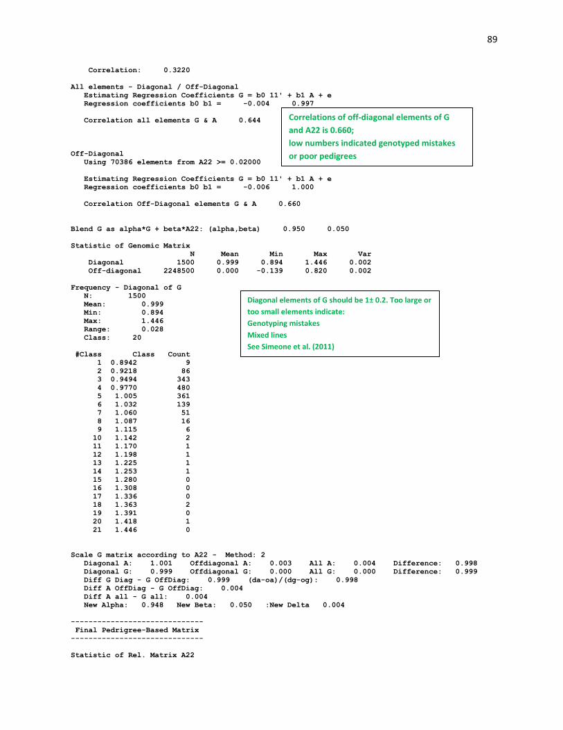
89
Correlation: 0.3220
All elements - Diagonal / Off-Diagonal
Estimating Regression Coefficients G = b0 11' + b1 A + e
Regression coefficients b0 b1 = -0.004 0.997
Correlation all elements G & A 0.644
Off-Diagonal
Using 70386 elements from A22 >= 0.02000
Estimating Regression Coefficients G = b0 11' + b1 A + e
Regression coefficients b0 b1 = -0.006 1.000
Correlation Off-Diagonal elements G & A 0.660
Blend G as alpha*G + beta*A22: (alpha,beta) 0.950 0.050
Statistic of Genomic Matrix
N Mean Min Max Var
Diagonal 1500 0.999 0.894 1.446 0.002
Off-diagonal 2248500 0.000 -0.139 0.820 0.002
Frequency - Diagonal of G
N: 1500
Mean: 0.999
Min: 0.894
Max: 1.446
Range: 0.028
Class: 20
#Class Class Count
1 0.8942 9
2 0.9218 86
3 0.9494 343
4 0.9770 480
5 1.005 361
6 1.032 139
7 1.060 51
8 1.087 16
9 1.115 6
10 1.142 2
11 1.170 1
12 1.198 1
13 1.225 1
14 1.253 1
15 1.280 0
16 1.308 0
17 1.336 0
18 1.363 2
19 1.391 0
20 1.418 1
21 1.446 0
Scale G matrix according to A22 - Method: 2
Diagonal A: 1.001 Offdiagonal A: 0.003 All A: 0.004 Difference: 0.998
Diagonal G: 0.999 Offdiagonal G: 0.000 All G: 0.000 Difference: 0.999
Diff G Diag - G OffDiag: 0.999 (da-oa)/(dg-og): 0.998
Diff A OffDiag - G OffDiag: 0.004
Diff A all - G all: 0.004
New Alpha: 0.948 New Beta: 0.050 :New Delta 0.004
------------------------------
Final Pedrigree-Based Matrix
------------------------------
Statistic of Rel. Matrix A22
Correlations of off-diagonal elements of G
and A22 is 0.660;
low numbers indicated genotyped mistakes
or poor pedigrees
Diagonal elements of G should be 1± 0.2. Too large or
too small elements indicate:
- Genotyping mistakes
- Mixed lines
See Simeone et al. (2011)

90
N Mean Min Max Var
Diagonal 1500 1.001 1.000 1.250 0.000
Off-diagonal 2248500 0.003 0.000 0.750 0.001
----------------------
Final Genomic Matrix
----------------------
Statistic of Genomic Matrix
N Mean Min Max Var
Diagonal 1500 1.001 0.896 1.447 0.002
Off-diagonal 2248500 0.003 -0.134 0.822 0.002
Correlation of Genomic Inbreeding and Pedigree Inbreeding
Correlation: 0.3363
All elements - Diagonal / Off-Diagonal
Estimating Regression Coefficients G = b0 11' + b1 A + e
Regression coefficients b0 b1 = 0.000 0.995
Correlation all elements G & A 0.663
Off-Diagonal
Using 70386 elements from A22 >= 0.02000
Estimating Regression Coefficients G = b0 11' + b1 A + e
Regression coefficients b0 b1 = -0.001 0.998
Correlation Off-Diagonal elements G & A 0.679
Creating A22-inverse
Wall time: 08-05-2011 16h 58m 10s 866
Inverse using ginv2
elapsed time 3.54446100000000
Wall time: 08-05-2011 16h 58m 17s 691
Statistic of Inv. Rel. Matrix A22
N Mean Min Max Var
Diagonal 1500 1.607 1.056 9.221 0.575
Off-diagonal 2248500 -0.001 -1.067 0.533 0.001
Creating G-inverse
Wall time: 08-05-2011 16h 58m 17s 987
Inverse using ginv2
elapsed time 4.24635400000000
Wall time: 08-05-2011 16h 58m 26s 044
Statistic of Inv. Genomic Matrix
N Mean Min Max Var
Diagonal 1500 8.007 3.597 64.893 21.055
Off-diagonal 2248500 -0.005 -12.697 6.632 0.056
Creating GimA22i in file: "GimA22i"
Calculating GmA22/GimA22i Matrix Densem storage
Calculating GmA22/GimA22i Matrix...elapsed time 0.1269817
Statistics of G after scaling as in Chen et al (2011) or Vitezica et al. (2011)
Statistics should be same as for A22.
Statistics of A22-1
Statistics of G-1
2 x diag(G-1 - A22-1) is approx. measure of extra genomic info in terms of effective daughters

91
Setup Genomic Done.
wGimA22i 1.00000000000000
hash matrix increased from 100000 to 150000 % filled: 0.9000
hash matrix increased from 150000 to 225000 % filled: 0.9000
hash matrix increased from 225000 to 337500 % filled: 0.9000
hash matrix increased from 337500 to 506250 % filled: 0.9000
hash matrix increased from 506250 to 759375 % filled: 0.9000
hash matrix increased from 759375 to 1139062 % filled: 0.9000
hash matrix increased from 1139062 to 1708593 % filled: 0.9000
finished peds in 30.68333 s, 1193064 nonzeroes
round 1 convergence= 3.234776127905992E-004
round 2 convergence= 1.615955145159698E-005
round 3 convergence= 9.675137058360991E-006
round 4 convergence= 6.533482675941447E-006
round 5 convergence= 2.711751165983321E-006
………..
………..
round 64 convergence= 2.721030958617683E-012
round 65 convergence= 1.931029578758311E-012
round 66 convergence= 1.610472992188148E-012
round 67 convergence= 1.259204136643006E-012
round 68 convergence= 9.025592862452768E-013
68 iterations, convergence criterion= 9.025592862452768E-013
solutions stored in file: "solutions"
solutions
trait/effect level solution
1 1 1 4.97591211
1 2 1 0.10194865
1 2 2 0.33749439
1 2 3 0.04475742
1 2 4 -0.31055520
1 2 5 0.22368631
1 2 6 -0.09454804
1 2 7 -0.03186435
1 2 8 0.18033163
name of parameter file?renf90.par
* SNP file: marker.geno.clean
* SNP Xref file: marker.geno.clean_XrefID
* Frequency to Center Z=M-p to create G=ZZ'/k (default whichfreq = 2):
2
AI-REMLF90 ver. 1.96
Parameter file: renf90.par
Data file: renf90.dat
Number of Traits 1
Number of Effects 2
Position of Observations 1
Position of Weight (1) 0
Value of Missing Trait/Observation 0
………..
………..
Statistic of Inv. Genomic Matrix
N Mean Min Max Var
Diagonal 1500 8.007 3.597 64.893 21.055
Off-diagonal 2248500 -0.005 -12.697 6.632 0.056
Creating GimA22i in file: "GimA22i"
Solution file
Variance component estimation by AIREMLF90

92
Calculating GmA22/GimA22i Matrix Densem storage
Calculating GmA22/GimA22i Matrix...elapsed time 0.1089821
Setup Genomic Done.
wGimA22i 1.00000000000000
hash matrix increased from 85428 to 128142 % filled: 0.9000
hash matrix increased from 128142 to 192213 % filled: 0.9000
hash matrix increased from 192213 to 288319 % filled: 0.9000
hash matrix increased from 288319 to 432478 % filled: 0.9000
hash matrix increased from 432478 to 648717 % filled: 0.9000
hash matrix increased from 648717 to 973075 % filled: 0.9000
hash matrix increased from 973075 to 1459612 % filled: 0.9000
finished peds in 32.01313 s, 1193064 nonzeroes
rank= 15801
**************
**** FSPAK ***
**************
MPE / IM / MAE
Jun 1994
SPARSE STATISTICS
DIMENSION OF MATRIX = 15801
RANK = 15801
STORAGE AVAILABLE = 7061497
MAXIMUM NEEDED = 7061497
NZE IN UPPER TRIANGULAR = 1208865
NZE IN FACTOR = 1521840
NO. OF CALLS NUM FACT = 1
NO. OF CALLS SOLVE = 1
NO. OF CALLS SPARS SOLV = 0
NO. OF CALLS DET / LDET = 1
NO. OF CALLS SPARS INV = 1
TOTAL CPU TIME IN FSPAK = 9.465561
TIME FOR FINDING ORDER = 2.568611
TIME FOR SYMBOLIC FAC = 0.676899
TIME FOR NUMERICAL FAC = 2.017693
TIME FOR SOLVE = 0.008995
TIME FOR SPARSE SOLVE = 0.000000
TIME FOR SPARSE INVERSE = 4.147369
-2logL = 43515.7413644011 : AIC = 43519.7413644011
In round 1 convergence= 0.423851780381002
delta convergence= 0.252173522062583
new R
0.58510
new G
0.28516
-2logL = 53013.2734486053 : AIC = 53017.2734486053
In round 2 convergence= 0.141351613622645
delta convergence= 0.117430758820623
new R
0.52205
new G
0.45696
-2logL = 52800.6601605267 : AIC = 52804.6601605267
In round 3 convergence= 1.725330565925358E-002
delta convergence= 4.769938966058494E-002
new R
0.49575
new G
0.52606
-2logL = 52785.2479463395 : AIC = 52789.2479463395
In round 4 convergence= 1.101891763451498E-004
delta convergence= 3.662497104484009E-003
new R
0.49400

93
new G
0.53164
-2logL = 52785.1635385807 : AIC = 52789.1635385807
In round 5 convergence= 2.804695847240073E-009
delta convergence= 1.777604045032979E-005
new R
0.49400
new G
0.53167
Final Estimates
Genetic variance(s) for effect 2
0.53167
Residual variance(s)
0.49400
inverse of AI matrix (Sampling Variance)
0.40448E-03 -0.17367E-03
-0.17367E-03 0.14702E-03
Correlations from inverse of AI matrix
1.0000 -0.71219
-0.71219 1.0000
SE for R
0.12125E-01
SE for G
0.20112E-01
solutions stored in file: "solutions"
Estimates of variance components

94
Appendix I (complete genomic analysis)
Data files are available at http://nce.ads.uga.edu/wiki/doku.php?id=course_materials_-
_from_uga_2014.
Using RENUMF90, PREGSF90, BLUPF90 (BLUP), BLUPF90 (ssGBLUP), PREDICTF90, POSTGSF90 (ssGWAS)
Simulated data
Single trait with heritability of 0.30 and phenotypic variance = 1.0
Five generations
Total of 994 parents from generations 1 to 4 were genotyped
Three hundred progeny from 5th generation had genotypes and pedigree, but phenotypes were
removed for traditional and genomic evaluations
Data Structure:
#Animal Generation Sex Mu QTL Residual Phenotype (Phenotype = Mu + QTL + Residual) 1 0 1 1 -0.826104 1.586661 1.76056
2 0 1 1 -1.093034 -0.451821 -0.544855
3 0 1 1 -0.135824 0.984936 1.84911
4 0 1 1 0.044242 -0.802145 0.242097
5 0 1 1 0.342068 0.028434 1.3705
.
.
6095 5 1 1 1.801324 -0.494822 2.3065
6096 5 2 1 0.772964 0.791936 2.5649
6097 5 2 1 0.748241 0.285815 2.03406
6098 5 1 1 1.042522 -1.606656 0.435866
6099 5 1 1 0.891319 0.179843 2.07116
6100 5 1 1 0.745873 0.034715 1.78059
Pedigree: 6100 animals
#Animal Sire Dam 1 0 0
2 0 0
3 0 0
4 0 0
5 0 0
.
.
6095 4576 4403
6096 4576 4065
6097 4576 2263
6098 4576 4150
6099 4576 3690
6100 4576 4311
Genotypes: 1294 animals genotyped for 1000 SNP across 5 chromosomes
# Animal SNP1SNP2SNP3SNP4SNP5…SNP1000 6100 22212…1

95
Map:
#SNP order chromosome position 1 1 10010
2 1 16722
3 1 33444
4 1 50166
5 1 66888
.
.
1000 5 299878
Parameter file for RENUMF90 DATAFILE
newdata.txt
TRAITS
7
FIELDS_PASSED TO OUTPUT
2
WEIGHT(S)
RESIDUAL_VARIANCE
0.70
EFFECT
4 cross alpha #mu
EFFECT
1 cross alpha #animal
RANDOM
animal
FILE
ped.txt
FILE_POS
1 2 3 0 0
SNP_FILE
snp.txt
PED_DEPTH
0
(CO)VARIANCES
0.30
OPTION chrinfo map.txt
Log file for RENUMF90 RENUMF90 version 1.104
name of parameter file? renum.par
datafile:newdata.txt
traits: 7
fields passed: 2
R
0.7000
Processing effect 1 of type cross
item_kind=alpha
Processing effect 2 of type cross

96
item_kind=alpha
pedigree file name "ped.txt"
positions of animal, sire, dam, alternate dam and yob 1 2 3 0 0
SNP file name "snp.txt"
all pedigrees to be included
Reading (CO)VARIANCES: 1 x 1
Maximum size of character fields: 20
Maximum size of record (max_string_readline): 800
Maximum number of fields for input file (max_field_readline): 100
hash tables for effects set up
read 6100 records
table with 1 elements sorted
added count
Effect group 1 of column 1 with 1 levels
table expanded from 10000 to 10000 records
added count
Effect group 2 of column 1 with 6100 levels
wrote statistics in file "renf90.tables"
Basic statistics for input data (missing value code is 0)
Pos Min Max Mean SD N
7 -2.8883 5.0863 1.0042 0.99034 6100
random effect with SNPs 2
type: animal
file: snp.txt
read SNPs 1294 records
Effect group 2 of column 1 with 6100 levels
random effect 2
type:animal
opened output pedigree file "renadd02.ped"
read 6100 pedigree records
Pedigree checks
Number of animals with records: 6100
Number of animals with genotypes: 1294
Number of animals with records or genotypes: 6100
Number of animals with genotypes and no records 0
Number of parents without records or genotypes: 0
Total number of animals: 6100
Wrote cross reference IDs for SNP file "snp.txt_XrefID"
Wrote parameter file "renf90.par"
Wrote renumbered data "renf90.dat"
Parameter file for PREGSF90 without quality control DATAFILE
renf90.dat
NUMBER_OF_TRAITS
1
NUMBER_OF_EFFECTS
2

97
OBSERVATION(S)
1
WEIGHT(S)
EFFECTS: POSITIONS_IN_DATAFILE NUMBER_OF_LEVELS TYPE_OF_EFFECT[EFFECT NESTED]
2 1 cross
3 6100 cross
RANDOM_RESIDUAL VALUES
0.70000
RANDOM_GROUP
2
RANDOM_TYPE
add_animal
FILE
renadd02.ped
(CO)VARIANCES
0.30000
OPTION SNP_file snp.txt
OPTION chrinfo map.txt
OPTION no_quality_control
Log file for PREGSF90 without quality control name of parameter file?
renf90.par
preGS 1.10
Parameter file: renf90.par
Data file: renf90.dat
Number of Traits 1
Number of Effects 2
Position of Observations 1
Position of Weight (1) 0
Value of Missing Trait/Observation 0
EFFECTS
# type position (2) levels [positions for nested]
1 cross-classified 2 1
2 cross-classified 3 6100
Residual (co)variance Matrix
0.70000
Random Effect(s) 2
Type of Random Effect: additive animal
Pedigree File: renadd02.ped
trait effect (CO)VARIANCES
1 2 0.3000
REMARKS
(1) Weight position 0 means no weights utilized
(2) Effect positions of 0 for some effects and traits means that such
effects are missing for specified traits
Options read from parameter file:
* SNP file: snp.txt
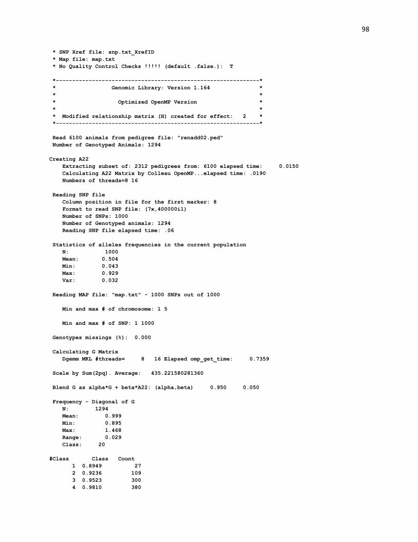
98
* SNP Xref file: snp.txt_XrefID
* Map file: map.txt
* No Quality Control Checks !!!!! (default .false.): T
*--------------------------------------------------------------*
* Genomic Library: Version 1.164 *
* *
* Optimized OpenMP Version *
* *
* Modified relationship matrix (H) created for effect: 2 *
*--------------------------------------------------------------*
Read 6100 animals from pedigree file: "renadd02.ped"
Number of Genotyped Animals: 1294
Creating A22
Extracting subset of: 2312 pedigrees from: 6100 elapsed time: 0.0150
Calculating A22 Matrix by Colleau OpenMP...elapsed time: .0190
Numbers of threads=8 16
Reading SNP file
Column position in file for the first marker: 8
Format to read SNP file: (7x,400000i1)
Number of SNPs: 1000
Number of Genotyped animals: 1294
Reading SNP file elapsed time: .06
Statistics of alleles frequencies in the current population
N: 1000
Mean: 0.504
Min: 0.043
Max: 0.929
Var: 0.032
Reading MAP file: "map.txt" - 1000 SNPs out of 1000
Min and max # of chromosome: 1 5
Min and max # of SNP: 1 1000
Genotypes missings (%): 0.000
Calculating G Matrix
Dgemm MKL #threads= 8 16 Elapsed omp_get_time: 0.7359
Scale by Sum(2pq). Average: 435.221580281360
Blend G as alpha*G + beta*A22: (alpha,beta) 0.950 0.050
Frequency - Diagonal of G
N: 1294
Mean: 0.999
Min: 0.895
Max: 1.468
Range: 0.029
Class: 20
#Class Class Count
1 0.8949 27
2 0.9236 109
3 0.9523 300
4 0.9810 380

99
5 1.010 287
6 1.038 137
7 1.067 33
8 1.096 14
9 1.124 3
10 1.153 1
11 1.182 0
12 1.210 2
13 1.239 0
14 1.268 0
15 1.296 0
16 1.325 0
17 1.354 0
18 1.382 0
19 1.411 0
20 1.440 1
21 1.468 0
Check for diagonal of genomic relationship matrix
Check for diagonal of genomic relationship matrix, genotypes not removed: 0
------------------------------
Final Pedrigree-Based Matrix
------------------------------
Statistic of Rel. Matrix A22
N Mean Min Max Var
Diagonal 1294 1.001 1.000 1.250 0.000
Off-diagonal 1673142 0.005 0.000 0.750 0.001
----------------------
Final Genomic Matrix
----------------------
Statistic of Genomic Matrix
N Mean Min Max Var
Diagonal 1294 1.001 0.898 1.469 0.002
Off-diagonal 1673142 0.005 -0.158 0.791 0.002
Correlation of Genomic Inbreeding and Pedigree Inbreeding
Correlation: 0.2177
All elements - Diagonal / Off-Diagonal
Estimating Regression Coefficients G = b0 11' + b1 A + e
Regression coefficients b0 b1 = 0.000 0.991
Correlation all elements G & A 0.717
Off-Diagonal
Using 83426 elements from A22 >= .02000
Estimating Regression Coefficients G = b0 11' + b1 A + e
Regression coefficients b0 b1 = -0.003 0.999
Correlation Off-Diagonal elements G & A 0.777
Creating A22-inverse
Inverse LAPACK MKL dpotrf/i #threads= 8 16 Elapsed omp_get_time: 0.1071
----------------------
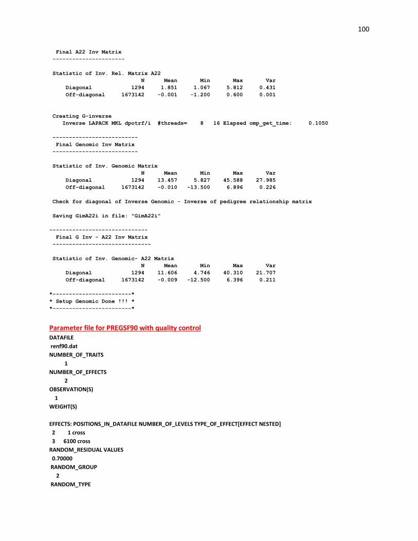
100
Final A22 Inv Matrix
----------------------
Statistic of Inv. Rel. Matrix A22
N Mean Min Max Var
Diagonal 1294 1.851 1.067 5.812 0.431
Off-diagonal 1673142 -0.001 -1.200 0.600 0.001
Creating G-inverse
Inverse LAPACK MKL dpotrf/i #threads= 8 16 Elapsed omp_get_time: 0.1050
--------------------------
Final Genomic Inv Matrix
--------------------------
Statistic of Inv. Genomic Matrix
N Mean Min Max Var
Diagonal 1294 13.457 5.827 45.588 27.985
Off-diagonal 1673142 -0.010 -13.500 6.896 0.226
Check for diagonal of Inverse Genomic - Inverse of pedigree relationship matrix
Saving GimA22i in file: "GimA22i"
------------------------------
Final G Inv - A22 Inv Matrix
------------------------------
Statistic of Inv. Genomic- A22 Matrix
N Mean Min Max Var
Diagonal 1294 11.606 4.746 40.310 21.707
Off-diagonal 1673142 -0.009 -12.500 6.396 0.211
*------------------------*
* Setup Genomic Done !!! *
*------------------------*
Parameter file for PREGSF90 with quality control DATAFILE
renf90.dat
NUMBER_OF_TRAITS
1
NUMBER_OF_EFFECTS
2
OBSERVATION(S)
1
WEIGHT(S)
EFFECTS: POSITIONS_IN_DATAFILE NUMBER_OF_LEVELS TYPE_OF_EFFECT[EFFECT NESTED]
2 1 cross
3 6100 cross
RANDOM_RESIDUAL VALUES
0.70000
RANDOM_GROUP
2
RANDOM_TYPE
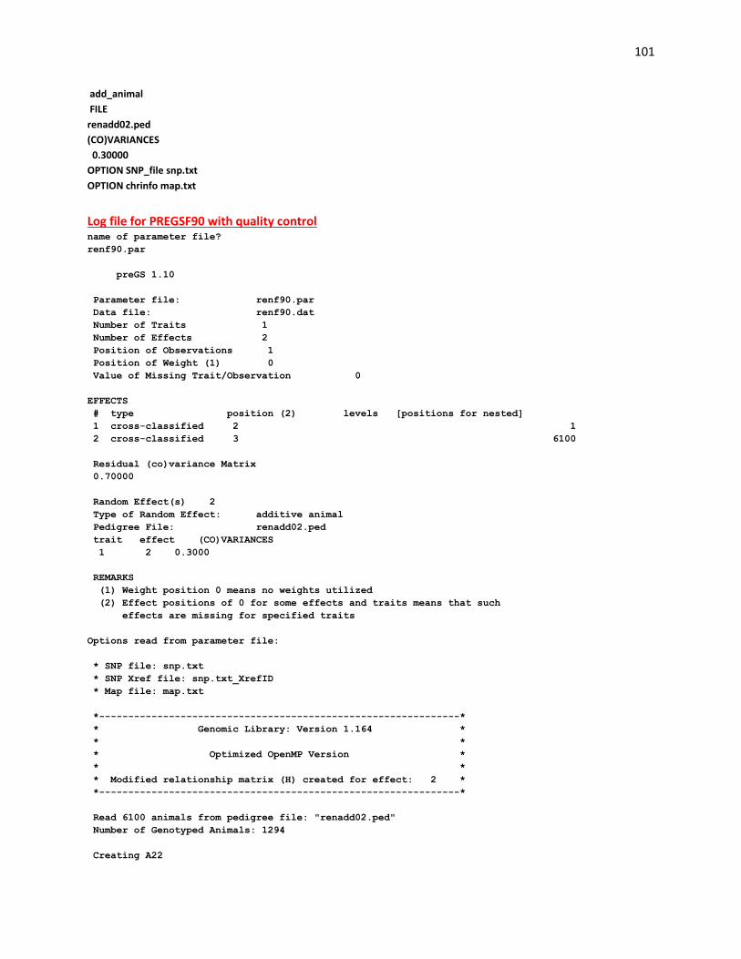
101
add_animal
FILE
renadd02.ped
(CO)VARIANCES
0.30000
OPTION SNP_file snp.txt
OPTION chrinfo map.txt
Log file for PREGSF90 with quality control name of parameter file?
renf90.par
preGS 1.10
Parameter file: renf90.par
Data file: renf90.dat
Number of Traits 1
Number of Effects 2
Position of Observations 1
Position of Weight (1) 0
Value of Missing Trait/Observation 0
EFFECTS
# type position (2) levels [positions for nested]
1 cross-classified 2 1
2 cross-classified 3 6100
Residual (co)variance Matrix
0.70000
Random Effect(s) 2
Type of Random Effect: additive animal
Pedigree File: renadd02.ped
trait effect (CO)VARIANCES
1 2 0.3000
REMARKS
(1) Weight position 0 means no weights utilized
(2) Effect positions of 0 for some effects and traits means that such
effects are missing for specified traits
Options read from parameter file:
* SNP file: snp.txt
* SNP Xref file: snp.txt_XrefID
* Map file: map.txt
*--------------------------------------------------------------*
* Genomic Library: Version 1.164 *
* *
* Optimized OpenMP Version *
* *
* Modified relationship matrix (H) created for effect: 2 *
*--------------------------------------------------------------*
Read 6100 animals from pedigree file: "renadd02.ped"
Number of Genotyped Animals: 1294
Creating A22

102
Extracting subset of: 2312 pedigrees from: 6100 elapsed time: 0.0160
Calculating A22 Matrix by Colleau OpenMP...elapsed time: .0189
Numbers of threads=8 16
Reading SNP file
Column position in file for the first marker: 8
Format to read SNP file: (7x,400000i1)
Number of SNPs: 1000
Number of Genotyped animals: 1294
Reading SNP file elapsed time: .06
Statistics of alleles frequencies in the current population
N: 1000
Mean: 0.504
Min: 0.043
Max: 0.929
Var: 0.032
Reading MAP file: "map.txt" - 1000 SNPs out of 1000
Min and max # of chromosome: 1 5
Min and max # of SNP: 1 1000
Quality Control - SNPs with Call Rate < callrate ( 0.90) will removed: 0
Quality Control - SNPs with MAF < minfreq ( 0.05) will removed: 1
Quality Control - Monomorphic SNPs will be removed: 0
Quality Control - Removed Animals with Call rate < callrate ( 0.90): 0
Quality Control - Check Parent-Progeny Mendelian conflicts
Total animals: 6100 - Genotyped animals: 1294 - Effective: 1294
Number of pairs Individual - Sire: 450
Number of pairs Individual - Dam: 440
Number of trios Individual - Sire - Dam: 206
No sex Chromosome information is available
Parent-progeny conflicts or HWE could eliminate SNPs in sex Chr
Provide map information and sex Chr to checks using autosomes
Checking SNPs for Mendelian conflicts
Total number of effective SNP: 999
Total number of parent-progeny evaluations: 890
Number of SNPs with Mendelian conflicts: 0
Checking Animals for Mendelian conflicts
Total number of effective SNP for checks on Animals: 999
Number of Parent-Progeny Mendelian Conflicts: 0
Number of effective SNPs (after QC): 999
Number of effective Indiviuals (after QC): 1294
Statistics of alleles frequencies in the current population after
Quality Control (MAF, monomorphic, call rate, HWE, Mendelian conflicts)

103
N: 999
Mean: 0.504
Min: 0.051
Max: 0.929
Var: 0.032
Genotypes missings (%): 0.100
Genotypes missings after cleannig (%): 0.000
Calculating G Matrix
Dgemm MKL #threads= 8 16 Elapsed omp_get_time: 0.9840
Scale by Sum(2pq). Average: 435.140185710293
Blend G as alpha*G + beta*A22: (alpha,beta) 0.950 0.050
Frequency - Diagonal of G
N: 1294
Mean: 0.999
Min: 0.895
Max: 1.469
Range: 0.029
Class: 20
#Class Class Count
1 0.8951 27
2 0.9238 109
3 0.9524 304
4 0.9811 379
5 1.010 285
6 1.038 137
7 1.067 32
8 1.096 14
9 1.125 3
10 1.153 1
11 1.182 0
12 1.211 2
13 1.239 0
14 1.268 0
15 1.297 0
16 1.325 0
17 1.354 0
18 1.383 0
19 1.411 0
20 1.440 1
21 1.469 0
Check for diagonal of genomic relationship matrix
Check for diagonal of genomic relationship matrix, genotypes not removed: 0
------------------------------
Final Pedrigree-Based Matrix
------------------------------
Statistic of Rel. Matrix A22
N Mean Min Max Var
Diagonal 1294 1.001 1.000 1.250 0.000
Off-diagonal 1673142 0.005 0.000 0.750 0.001
----------------------
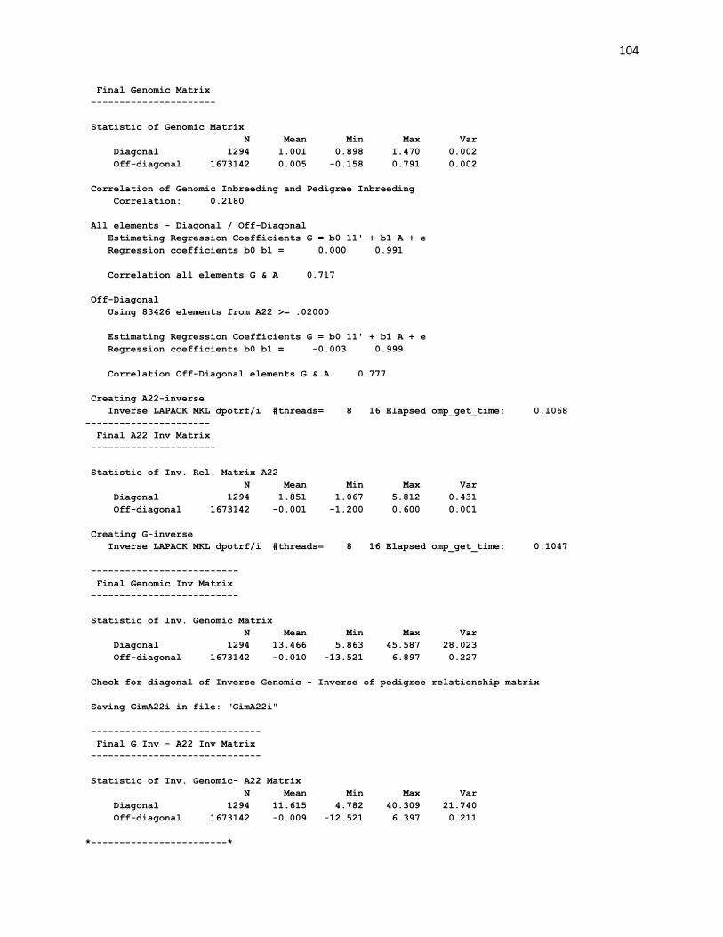
104
Final Genomic Matrix
----------------------
Statistic of Genomic Matrix
N Mean Min Max Var
Diagonal 1294 1.001 0.898 1.470 0.002
Off-diagonal 1673142 0.005 -0.158 0.791 0.002
Correlation of Genomic Inbreeding and Pedigree Inbreeding
Correlation: 0.2180
All elements - Diagonal / Off-Diagonal
Estimating Regression Coefficients G = b0 11' + b1 A + e
Regression coefficients b0 b1 = 0.000 0.991
Correlation all elements G & A 0.717
Off-Diagonal
Using 83426 elements from A22 >= .02000
Estimating Regression Coefficients G = b0 11' + b1 A + e
Regression coefficients b0 b1 = -0.003 0.999
Correlation Off-Diagonal elements G & A 0.777
Creating A22-inverse
Inverse LAPACK MKL dpotrf/i #threads= 8 16 Elapsed omp_get_time: 0.1068
----------------------
Final A22 Inv Matrix
----------------------
Statistic of Inv. Rel. Matrix A22
N Mean Min Max Var
Diagonal 1294 1.851 1.067 5.812 0.431
Off-diagonal 1673142 -0.001 -1.200 0.600 0.001
Creating G-inverse
Inverse LAPACK MKL dpotrf/i #threads= 8 16 Elapsed omp_get_time: 0.1047
--------------------------
Final Genomic Inv Matrix
--------------------------
Statistic of Inv. Genomic Matrix
N Mean Min Max Var
Diagonal 1294 13.466 5.863 45.587 28.023
Off-diagonal 1673142 -0.010 -13.521 6.897 0.227
Check for diagonal of Inverse Genomic - Inverse of pedigree relationship matrix
Saving GimA22i in file: "GimA22i"
------------------------------
Final G Inv - A22 Inv Matrix
------------------------------
Statistic of Inv. Genomic- A22 Matrix
N Mean Min Max Var
Diagonal 1294 11.615 4.782 40.309 21.740
Off-diagonal 1673142 -0.009 -12.521 6.397 0.211
*------------------------*

105
* Setup Genomic Done !!! *
*------------------------*
Parameter file for PREGSF90 with quality control, removing SNP from chromosome 5 and saving the
clean SNP file DATAFILE
renf90.dat
NUMBER_OF_TRAITS
1
NUMBER_OF_EFFECTS
2
OBSERVATION(S)
1
WEIGHT(S)
EFFECTS: POSITIONS_IN_DATAFILE NUMBER_OF_LEVELS TYPE_OF_EFFECT[EFFECT NESTED]
2 1 cross
3 6100 cross
RANDOM_RESIDUAL VALUES
0.70000
RANDOM_GROUP
2
RANDOM_TYPE
add_animal
FILE
renadd02.ped
(CO)VARIANCES
0.30000
OPTION SNP_file snp.txt
OPTION chrinfo map.txt
OPTION excludeCHR 5
OPTION saveCleanSNPs
Log file for PREGSF90 with quality control, removing SNP from chromosome 5 and saving the clean
SNP file name of parameter file?
renf90.par
preGS 1.10
Parameter file: renf90.par
Data file: renf90.dat
Number of Traits 1
Number of Effects 2
Position of Observations 1
Position of Weight (1) 0
Value of Missing Trait/Observation 0
EFFECTS
# type position (2) levels [positions for nested]
1 cross-classified 2 1
2 cross-classified 3 6100

106
Residual (co)variance Matrix
0.70000
Random Effect(s) 2
Type of Random Effect: additive animal
Pedigree File: renadd02.ped
trait effect (CO)VARIANCES
1 2 0.3000
REMARKS
(1) Weight position 0 means no weights utilized
(2) Effect positions of 0 for some effects and traits means that such
effects are missing for specified traits
Options read from parameter file:
* SNP file: snp.txt
* SNP Xref file: snp.txt_XrefID
* Map file: map.txt
* Save Clean SNP data to (SNP_file)_clean file (default .false.)
* Exclude Chromosomes (default .false.): 5
*--------------------------------------------------------------*
* Genomic Library: Version 1.164 *
* *
* Optimized OpenMP Version *
* *
* Modified relationship matrix (H) created for effect: 2 *
*--------------------------------------------------------------*
Read 6100 animals from pedigree file: "renadd02.ped"
Number of Genotyped Animals: 1294
Creating A22
Extracting subset of: 2312 pedigrees from: 6100 elapsed time: 0.0150
Calculating A22 Matrix by Colleau OpenMP...elapsed time: .0190
Numbers of threads=8 16
Reading SNP file
Column position in file for the first marker: 8
Format to read SNP file: (7x,400000i1)
Number of SNPs: 1000
Number of Genotyped animals: 1294
Reading SNP file elapsed time: .06
Statistics of alleles frequencies in the current population
N: 1000
Mean: 0.504
Min: 0.043
Max: 0.929
Var: 0.032
Reading MAP file: "map.txt" - 1000 SNPs out of 1000
Min and max # of chromosome: 1 5
Min and max # of SNP: 1 1000
Excluded 199 SNPs from 1 chromosomes: 5
Quality Control - SNPs with Call Rate < callrate ( 0.90) will removed: 199
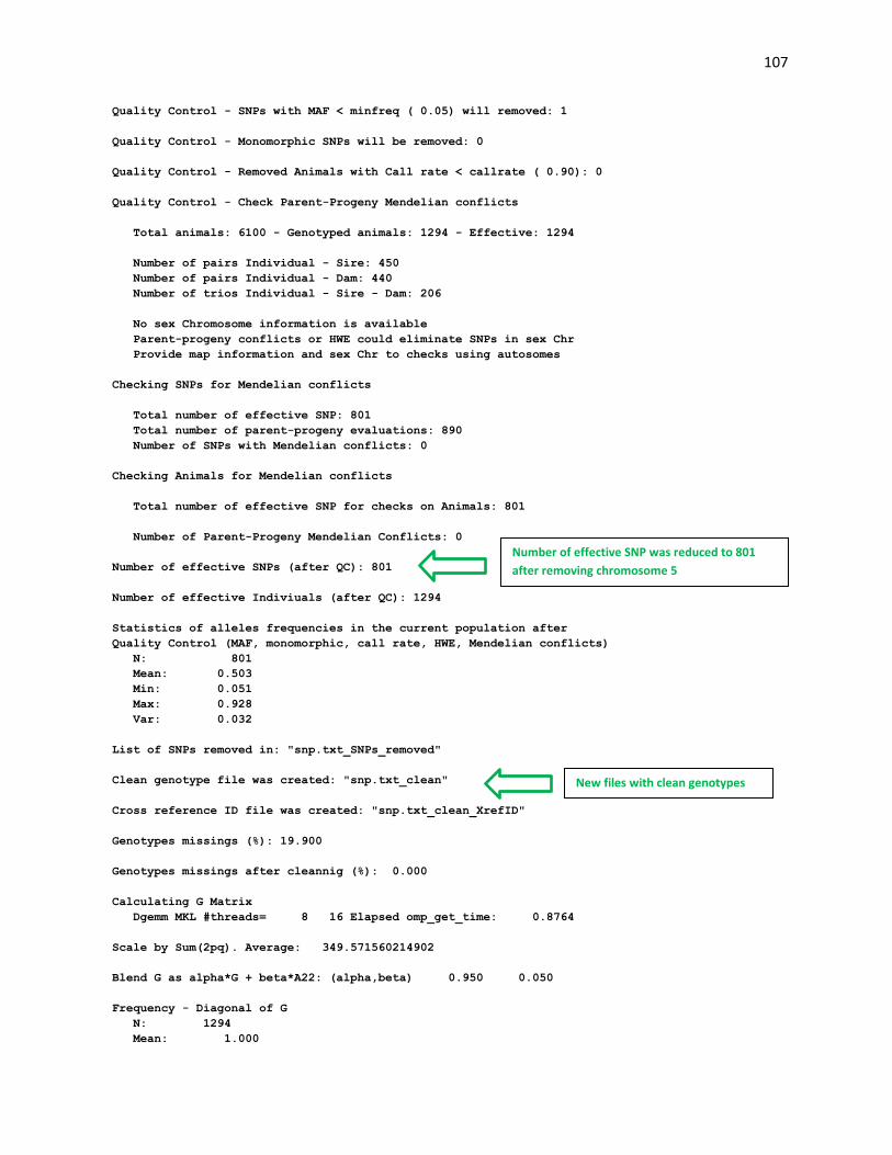
107
Quality Control - SNPs with MAF < minfreq ( 0.05) will removed: 1
Quality Control - Monomorphic SNPs will be removed: 0
Quality Control - Removed Animals with Call rate < callrate ( 0.90): 0
Quality Control - Check Parent-Progeny Mendelian conflicts
Total animals: 6100 - Genotyped animals: 1294 - Effective: 1294
Number of pairs Individual - Sire: 450
Number of pairs Individual - Dam: 440
Number of trios Individual - Sire - Dam: 206
No sex Chromosome information is available
Parent-progeny conflicts or HWE could eliminate SNPs in sex Chr
Provide map information and sex Chr to checks using autosomes
Checking SNPs for Mendelian conflicts
Total number of effective SNP: 801
Total number of parent-progeny evaluations: 890
Number of SNPs with Mendelian conflicts: 0
Checking Animals for Mendelian conflicts
Total number of effective SNP for checks on Animals: 801
Number of Parent-Progeny Mendelian Conflicts: 0
Number of effective SNPs (after QC): 801
Number of effective Indiviuals (after QC): 1294
Statistics of alleles frequencies in the current population after
Quality Control (MAF, monomorphic, call rate, HWE, Mendelian conflicts)
N: 801
Mean: 0.503
Min: 0.051
Max: 0.928
Var: 0.032
List of SNPs removed in: "snp.txt_SNPs_removed"
Clean genotype file was created: "snp.txt_clean"
Cross reference ID file was created: "snp.txt_clean_XrefID"
Genotypes missings (%): 19.900
Genotypes missings after cleannig (%): 0.000
Calculating G Matrix
Dgemm MKL #threads= 8 16 Elapsed omp_get_time: 0.8764
Scale by Sum(2pq). Average: 349.571560214902
Blend G as alpha*G + beta*A22: (alpha,beta) 0.950 0.050
Frequency - Diagonal of G
N: 1294
Mean: 1.000
Number of effective SNP was reduced to 801
after removing chromosome 5
New files with clean genotypes

108
Min: 0.874
Max: 1.593
Range: 0.036
Class: 20
#Class Class Count
1 0.8741 17
2 0.9100 107
3 0.9460 341
4 0.9819 419
5 1.018 281
6 1.054 98
7 1.090 20
8 1.126 4
9 1.162 4
10 1.198 1
11 1.234 0
12 1.270 1
13 1.306 0
14 1.342 0
15 1.377 0
16 1.413 0
17 1.449 0
18 1.485 0
19 1.521 0
20 1.557 1
21 1.593 0
Check for diagonal of genomic relationship matrix
Check for diagonal of genomic relationship matrix, genotypes not removed: 0
------------------------------
Final Pedrigree-Based Matrix
------------------------------
Statistic of Rel. Matrix A22
N Mean Min Max Var
Diagonal 1294 1.001 1.000 1.250 0.000
Off-diagonal 1673142 0.005 0.000 0.750 0.001
----------------------
Final Genomic Matrix
----------------------
Statistic of Genomic Matrix
N Mean Min Max Var
Diagonal 1294 1.001 0.876 1.593 0.002
Off-diagonal 1673142 0.005 -0.169 0.861 0.003
Correlation of Genomic Inbreeding and Pedigree Inbreeding
Correlation: 0.2092
All elements - Diagonal / Off-Diagonal
Estimating Regression Coefficients G = b0 11' + b1 A + e
Regression coefficients b0 b1 = 0.000 0.991
Correlation all elements G & A 0.677
Off-Diagonal
Using 83426 elements from A22 >= .02000

109
Estimating Regression Coefficients G = b0 11' + b1 A + e
Regression coefficients b0 b1 = -0.002 0.996
Correlation Off-Diagonal elements G & A 0.742
Creating A22-inverse
Inverse LAPACK MKL dpotrf/i #threads= 8 16 Elapsed omp_get_time: 0.1409
----------------------
Final A22 Inv Matrix
----------------------
Statistic of Inv. Rel. Matrix A22
N Mean Min Max Var
Diagonal 1294 1.851 1.067 5.812 0.431
Off-diagonal 1673142 -0.001 -1.200 0.600 0.001
Creating G-inverse
Inverse LAPACK MKL dpotrf/i #threads= 8 16 Elapsed omp_get_time: 0.1370
--------------------------
Final Genomic Inv Matrix
--------------------------
Statistic of Inv. Genomic Matrix
N Mean Min Max Var
Diagonal 1294 17.075 7.840 56.092 43.645
Off-diagonal 1673142 -0.013 -16.499 8.893 0.309
Check for diagonal of Inverse Genomic - Inverse of pedigree relationship matrix
Saving GimA22i in file: "GimA22i"
------------------------------
Final G Inv - A22 Inv Matrix
------------------------------
Statistic of Inv. Genomic- A22 Matrix
N Mean Min Max Var
Diagonal 1294 15.223 6.759 51.043 35.648
Off-diagonal 1673142 -0.012 -15.499 8.393 0.289
*------------------------*
* Setup Genomic Done !!! *
*------------------------*
Parameter file for PREGSF90 with quality control and PCA analysis
Include extra option: OPTION plotpca

110
Parameter file for BLUPF90 without genomic information DATAFILE
renf90_5.dat
NUMBER_OF_TRAITS
1
NUMBER_OF_EFFECTS
2
OBSERVATION(S)
1
WEIGHT(S)
EFFECTS: POSITIONS_IN_DATAFILE NUMBER_OF_LEVELS TYPE_OF_EFFECT[EFFECT NESTED]
2 1 cross
3 6100 cross
RANDOM_RESIDUAL VALUES
0.70000
RANDOM_GROUP
2
RANDOM_TYPE
add_animal
FILE
renadd02.ped
(CO)VARIANCES
0.30000
OPTION conv_crit 1e-15
Log file for BLUPF90 without genomic information name of parameter file?
renf90_5.dat has phenotypes for all animals, but generation 5
Linux code to remove phenotypes for those animals:
awk '{ if ($4==5) print 0,$2,$3,$4; else print $1,$2,$3,$4}' renf90.dat > renf90_5.dat
Default convergence criteria = 1e-12
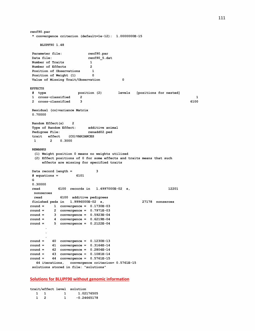
111
renf90.par
* convergence criterion (default=1e-12): 1.0000000E-15
BLUPF90 1.48
Parameter file: renf90.par
Data file: renf90_5.dat
Number of Traits 1
Number of Effects 2
Position of Observations 1
Position of Weight (1) 0
Value of Missing Trait/Observation 0
EFFECTS
# type position (2) levels [positions for nested]
1 cross-classified 2 1
2 cross-classified 3 6100
Residual (co)variance Matrix
0.70000
Random Effect(s) 2
Type of Random Effect: additive animal
Pedigree File: renadd02.ped
trait effect (CO)VARIANCES
1 2 0.3000
REMARKS
(1) Weight position 0 means no weights utilized
(2) Effect positions of 0 for some effects and traits means that such
effects are missing for specified traits
Data record length = 3
# equations = 6101
G
0.30000
read 6100 records in 1.4997000E-02 s, 12201
nonzeroes
read 6100 additive pedigrees
finished peds in 1.9996000E-02 s, 27178 nonzeroes
round = 1 convergence = 0.1730E-03
round = 2 convergence = 0.7971E-03
round = 3 convergence = 0.5923E-04
round = 4 convergence = 0.6219E-04
round = 5 convergence = 0.2122E-04
.
.
.
round = 40 convergence = 0.1230E-13
round = 41 convergence = 0.3164E-14
round = 42 convergence = 0.2804E-14
round = 43 convergence = 0.1081E-14
round = 44 convergence = 0.5761E-15
44 iterations, convergence criterion= 0.5761E-15
solutions stored in file: "solutions"
Solutions for BLUPF90 without genomic information
trait/effect level solution
1 1 1 1.02176505
1 2 1 -0.24665178

112
1 2 2 0.16420973
1 2 3 0.32371581
1 2 4 0.00318130
1 2 5 -0.13277100
EBV accuracy
If accuracy of EBV is desired, it can be calculated based on standard errors (se) for EBV.
BLUPF90 has an option for calculating se:
OPTION sol se
Solutions for BLUPF90 with option to calculate se
trait/effect level solution s.e.
1 1 1 1.02176504 0.02496866
1 2 1 -0.24665117 0.39158195
1 2 2 0.16421026 0.40488662
1 2 3 0.32371755 0.29405286
1 2 4 0.00318218 0.38229658
1 2 5 -0.13277154 0.46566701
Parameter file for BLUPF90 with genomic information (ssGBLUP) DATAFILE
renf90_5.dat
NUMBER_OF_TRAITS
1
NUMBER_OF_EFFECTS
2
OBSERVATION(S)
1
WEIGHT(S)
EFFECTS: POSITIONS_IN_DATAFILE NUMBER_OF_LEVELS TYPE_OF_EFFECT[EFFECT NESTED]
2 1 cross
3 6100 cross
RANDOM_RESIDUAL VALUES
0.70000
RANDOM_GROUP
2
RANDOM_TYPE
add_animal
FILE
renadd02.ped
(CO)VARIANCES
0.30000
OPTION SNP_file snp.txt
OPTION chrinfo map.txt
OPTION conv_crit 1e-15
The solution file (solutions) has 4 columns:
1) Trait [only 1 trait in this example]
2) Effect [we have 2 effects: overall mean (effect 1) and
additive genetic direct (effect 2)]
3) Level [number of the level for each effect in the model]
4) Solution
The solution file now includes a 5th
column with EBV standard errors

113
Log file for BLUPF90 with genomic information (ssGBLUP) name of parameter file?
renf90.par
* convergence criterion (default=1e-12): 1.0000000E-15
Options read from parameter file:
* SNP file: snp.txt
* SNP Xref file:snp.txt_XrefID
* Map file: map.txt
BLUPF90 1.48
Parameter file: renf90.par
Data file: renf90_5.dat
Number of Traits 1
Number of Effects 2
Position of Observations 1
Position of Weight (1) 0
Value of Missing Trait/Observation 0
EFFECTS
# type position (2) levels [positions for nested]
1 cross-classified 2 1
2 cross-classified 3 6100
Residual (co)variance Matrix
0.70000
Random Effect(s) 2
Type of Random Effect: additive animal
Pedigree File: renadd02.ped
trait effect (CO)VARIANCES
1 2 0.3000
REMARKS
(1) Weight position 0 means no weights utilized
(2) Effect positions of 0 for some effects and traits means that such
effects are missing for specified traits
Data record length = 3
# equations = 6101
G
0.30000
read 6100 records in 0.1499770 s, 12201
nonzeroes
read 6100 additive pedigrees
*--------------------------------------------------------------*
* Genomic Library: Version 1.164 *
* *
* Optimized OpenMP Version *
* *
* Modified relationship matrix (H) created for effect: 2 *
*--------------------------------------------------------------*
Read 6100 animals from pedigree file: "renadd02.ped"
Number of Genotyped Animals: 1294
Creating A22
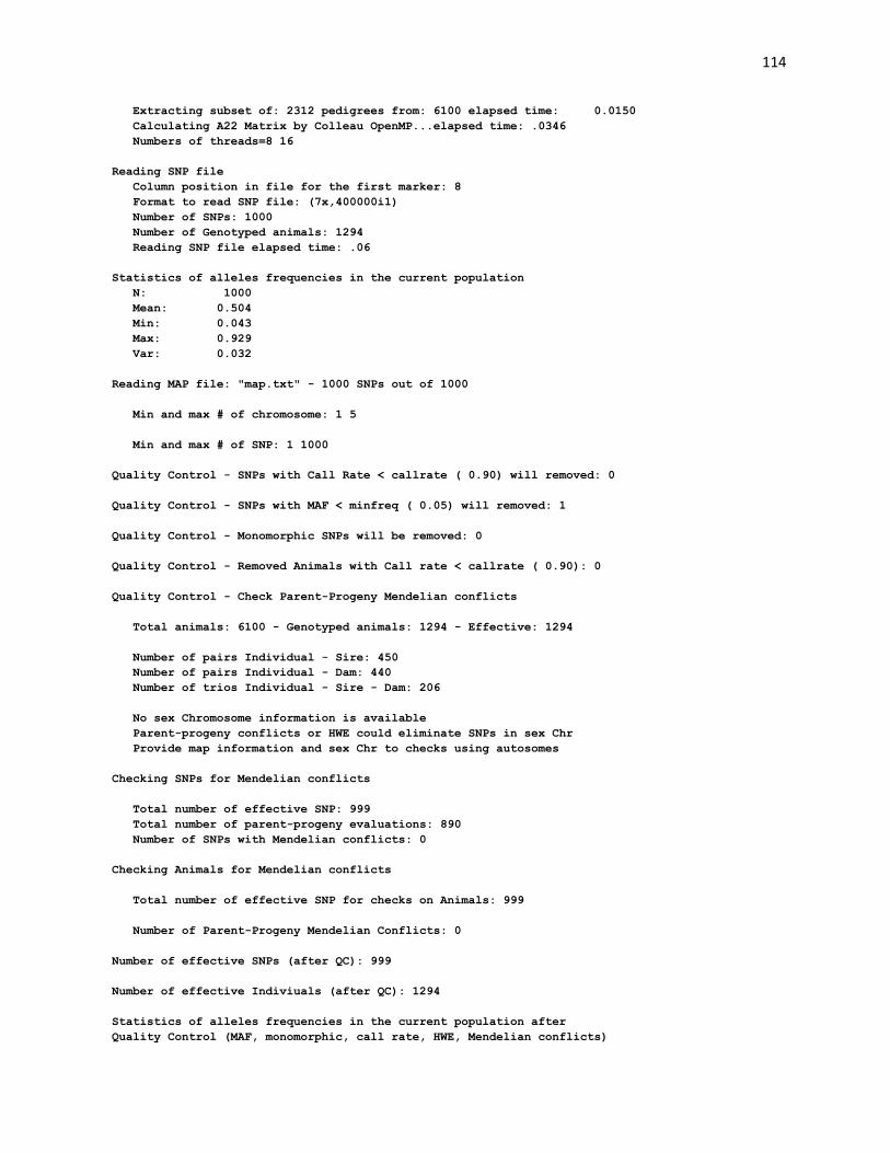
114
Extracting subset of: 2312 pedigrees from: 6100 elapsed time: 0.0150
Calculating A22 Matrix by Colleau OpenMP...elapsed time: .0346
Numbers of threads=8 16
Reading SNP file
Column position in file for the first marker: 8
Format to read SNP file: (7x,400000i1)
Number of SNPs: 1000
Number of Genotyped animals: 1294
Reading SNP file elapsed time: .06
Statistics of alleles frequencies in the current population
N: 1000
Mean: 0.504
Min: 0.043
Max: 0.929
Var: 0.032
Reading MAP file: "map.txt" - 1000 SNPs out of 1000
Min and max # of chromosome: 1 5
Min and max # of SNP: 1 1000
Quality Control - SNPs with Call Rate < callrate ( 0.90) will removed: 0
Quality Control - SNPs with MAF < minfreq ( 0.05) will removed: 1
Quality Control - Monomorphic SNPs will be removed: 0
Quality Control - Removed Animals with Call rate < callrate ( 0.90): 0
Quality Control - Check Parent-Progeny Mendelian conflicts
Total animals: 6100 - Genotyped animals: 1294 - Effective: 1294
Number of pairs Individual - Sire: 450
Number of pairs Individual - Dam: 440
Number of trios Individual - Sire - Dam: 206
No sex Chromosome information is available
Parent-progeny conflicts or HWE could eliminate SNPs in sex Chr
Provide map information and sex Chr to checks using autosomes
Checking SNPs for Mendelian conflicts
Total number of effective SNP: 999
Total number of parent-progeny evaluations: 890
Number of SNPs with Mendelian conflicts: 0
Checking Animals for Mendelian conflicts
Total number of effective SNP for checks on Animals: 999
Number of Parent-Progeny Mendelian Conflicts: 0
Number of effective SNPs (after QC): 999
Number of effective Indiviuals (after QC): 1294
Statistics of alleles frequencies in the current population after
Quality Control (MAF, monomorphic, call rate, HWE, Mendelian conflicts)
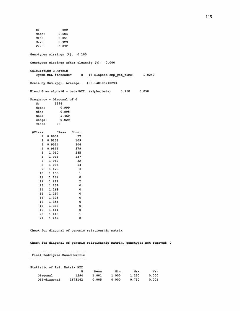
115
N: 999
Mean: 0.504
Min: 0.051
Max: 0.929
Var: 0.032
Genotypes missings (%): 0.100
Genotypes missings after cleannig (%): 0.000
Calculating G Matrix
Dgemm MKL #threads= 8 16 Elapsed omp_get_time: 1.0240
Scale by Sum(2pq). Average: 435.140185710293
Blend G as alpha*G + beta*A22: (alpha,beta) 0.950 0.050
Frequency - Diagonal of G
N: 1294
Mean: 0.999
Min: 0.895
Max: 1.469
Range: 0.029
Class: 20
#Class Class Count
1 0.8951 27
2 0.9238 109
3 0.9524 304
4 0.9811 379
5 1.010 285
6 1.038 137
7 1.067 32
8 1.096 14
9 1.125 3
10 1.153 1
11 1.182 0
12 1.211 2
13 1.239 0
14 1.268 0
15 1.297 0
16 1.325 0
17 1.354 0
18 1.383 0
19 1.411 0
20 1.440 1
21 1.469 0
Check for diagonal of genomic relationship matrix
Check for diagonal of genomic relationship matrix, genotypes not removed: 0
------------------------------
Final Pedrigree-Based Matrix
------------------------------
Statistic of Rel. Matrix A22
N Mean Min Max Var
Diagonal 1294 1.001 1.000 1.250 0.000
Off-diagonal 1673142 0.005 0.000 0.750 0.001
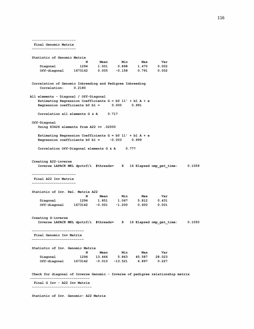
116
----------------------
Final Genomic Matrix
----------------------
Statistic of Genomic Matrix
N Mean Min Max Var
Diagonal 1294 1.001 0.898 1.470 0.002
Off-diagonal 1673142 0.005 -0.158 0.791 0.002
Correlation of Genomic Inbreeding and Pedigree Inbreeding
Correlation: 0.2180
All elements - Diagonal / Off-Diagonal
Estimating Regression Coefficients G = b0 11' + b1 A + e
Regression coefficients b0 b1 = 0.000 0.991
Correlation all elements G & A 0.717
Off-Diagonal
Using 83426 elements from A22 >= .02000
Estimating Regression Coefficients G = b0 11' + b1 A + e
Regression coefficients b0 b1 = -0.003 0.999
Correlation Off-Diagonal elements G & A 0.777
Creating A22-inverse
Inverse LAPACK MKL dpotrf/i #threads= 8 16 Elapsed omp_get_time: 0.1059
----------------------
Final A22 Inv Matrix
----------------------
Statistic of Inv. Rel. Matrix A22
N Mean Min Max Var
Diagonal 1294 1.851 1.067 5.812 0.431
Off-diagonal 1673142 -0.001 -1.200 0.600 0.001
Creating G-inverse
Inverse LAPACK MKL dpotrf/i #threads= 8 16 Elapsed omp_get_time: 0.1093
--------------------------
Final Genomic Inv Matrix
--------------------------
Statistic of Inv. Genomic Matrix
N Mean Min Max Var
Diagonal 1294 13.466 5.863 45.587 28.023
Off-diagonal 1673142 -0.010 -13.521 6.897 0.227
Check for diagonal of Inverse Genomic - Inverse of pedigree relationship matrix
------------------------------
Final G Inv - A22 Inv Matrix
------------------------------
Statistic of Inv. Genomic- A22 Matrix

117
N Mean Min Max Var
Diagonal 1294 11.615 4.782 40.309 21.740
Off-diagonal 1673142 -0.009 -12.521 6.397 0.211
*------------------------*
* Setup Genomic Done !!! *
*------------------------*
hash matrix increased from 131072 to 262144 % filled: 0.8000
hash matrix increased from 262144 to 524288 % filled: 0.8000
hash matrix increased from 524288 to 1048576 % filled: 0.8000
hash matrix increased from 1048576 to 2097152 % filled: 0.8000
finished peds in 25.61810 s, 861721 nonzeroes
round = 1 convergence = 0.6397E-03
round = 2 convergence = 0.4280E-03
round = 3 convergence = 0.3112E-03
round = 4 convergence = 0.9994E-04
round = 5 convergence = 0.8129E-04
.
.
.
round = 90 convergence = 0.3590E-14
round = 91 convergence = 0.2549E-14
round = 92 convergence = 0.2022E-14
round = 93 convergence = 0.1453E-14
round = 94 convergence = 0.9599E-15
94 iterations, convergence criterion= 0.9599E-15
solutions stored in file: "solutions"
Solutions for BLUPF90 with genomic information (ssGBLUP)
The solution file has the same format as in blupf90 without genomic information. The option for
calculating se for EBV can also be used here.
Parameter file for PREDICTF90
Predictivity can be measured as correlation between adjusted phenotypes and (G)EBV. In this example
we show how to use PREDICTF90 to adjust phenotypes for genotyped animals in the validation
population.
1) Adjusting phenotypes
As this program needs solution file, it can be run in the same folder as BLUP with complete data
Parameter file: DATAFILE
pred.dat
NUMBER_OF_TRAITS
1
NUMBER_OF_EFFECTS
2
OBSERVATION(S)
1
WEIGHT(S)
pred.dat is the data file only for genotyped animals
in 5th generation (validation animals). Lines can be
extracted from renf90.dat
118
EFFECTS: POSITIONS_IN_DATAFILE NUMBER_OF_LEVELS TYPE_OF_EFFECT[EFFECT NESTED]
2 1 cross
3 6100 cross
RANDOM_RESIDUAL VALUES
0.70000
RANDOM_GROUP
2
RANDOM_TYPE
add_animal
FILE
renadd02.ped
(CO)VARIANCES
0.30000
OPTION include_effects 2
Log file for adjusting phenotypes for genotyped animals in 5th generation name of parameter file?
pred.par
*** include effets to predict Yhat n, effects 1 2
PREDICTF90 1.3
Parameter file: gen.par
Data file: pred.dat
Number of Traits 1
Number of Effects 2
Position of Observations 1
Position of Weight (1) 0
Value of Missing Trait/Observation 0
EFFECTS
# type position (2) levels [positions for nested]
1 cross-classified 2 1
2 cross-classified 3 6100
Residual (co)variance Matrix
0.70000
Random Effect(s) 2
Type of Random Effect: additive animal
Pedigree File: renadd02.ped
trait effect (CO)VARIANCES
1 2 0.3000
REMARKS
(1) Weight position 0 means no weights utilized
(2) Effect positions of 0 for some effects and traits means that such
effects are missing for specified traits
Data record length = 3
# equations = 6101
*** effets to include in Yhat (T/F): F T
solutions read from file: soltutions
Animal Effect: 2
y(s), yhat(s), residual(s) in written in "yhat_residual" file
300 records read
Trait: 1 300
mean Y -5.204056186291079E-002 var Y 0.979795877964320

119
mean Yhat -1.187536126623551E-002 var Yhat 7.349890384221654E-002
cov (Y,Yhat) 8.232182257800019E-002 corr (Y,Yhat) 0.306765659847626
wrote bvs for animals in data in file "bvs.dat"
Output files from PREDICTF90
yhat_residual
4644 -0.266520 0.415535 0.339710
2176 -0.418925 0.094263 0.508577
bvs.dat
1 2 4644 0.415535
1 2 2176 0.094263
Hint: corr (Y,Yhat) from the output of PREDICTF90 (corr (Y,Yhat) 0.306765659847626) should not be
used as a measure of predictivity because it uses adjusted phenotypes and EBVs from the same dataset.
Usually, predictivity requires phenotypes adjusted for fixed effects in the complete data (benchmark)
and (G)EBVs calculated from the reduced data (without records for validation animals). The regular
predictivity measure is: corr[Y_from_PREDICTf90, (G)EBV_reduced]
For this small example with 1 trait, a general linux code to merge files is:
$awk '{print $1,$2}' ebv_complete/yhat_residual | sort +0 -1 > Y
$awk '{if ($2==2) print $3,$4}' ebv_reduced/solutions | sort +0 -1 >
ebv.temp
$awk '{if ($2==2) print $3,$4}' gebv_reduced/solutions | sort +0 -1 >
gebv.temp
$join -1 +1 -2 +1 Y ebv.temp > file1.temp
$join -1 +1 -2 +1 file1.temp gebv.temp > Y_ebv_gebv
An R code to calculate correlations is:
pred <- read.table(“Y_ebv_gebv”,header=F)
ebv_predictivity <- cor(pred[,2],pred[,3]); ebv_predictivity
gebv_predictivity <- cor(pred[,2],pred[,4]); gebv_predictivity
yhat_residual has 4 columns: animal | y | yhat | residual
Because OPTION include_effects 2 was used:
y is phenotype minus all effects other than animal
yhat receives the second effect, which is the animal effect
residual is phenotype minus animal effect
bvs.dat has 4 columns: trait | effect | Animal | solution (EBV)

120
Parameter files for GWAS using ssGBLUP (ssGWAS)
Run BLUPF90 with genomic information and salve G-1 and A22-1
DATAFILE
renf90.dat
NUMBER_OF_TRAITS
1
NUMBER_OF_EFFECTS
2
OBSERVATION(S)
1
WEIGHT(S)
EFFECTS: POSITIONS_IN_DATAFILE NUMBER_OF_LEVELS TYPE_OF_EFFECT[EFFECT NESTED]
2 1 cross
3 6100 cross
RANDOM_RESIDUAL VALUES
0.70000
RANDOM_GROUP
2
RANDOM_TYPE
add_animal
FILE
renadd02.ped
(CO)VARIANCES
0.30000
OPTION SNP_file snp.txt
OPTION chrinfo map.txt
OPTION no_quality_control
OPTION saveGInverse
OPTION saveA22Inverse
OPTION weightedG wei
Run POSTGSF90 and read G-1 and A22-1
DATAFILE
renf90.dat
NUMBER_OF_TRAITS
1
NUMBER_OF_EFFECTS
2
OBSERVATION(S)
1
WEIGHT(S)
EFFECTS: POSITIONS_IN_DATAFILE NUMBER_OF_LEVELS TYPE_OF_EFFECT[EFFECT NESTED]
2 1 cross
3 6100 cross
RANDOM_RESIDUAL VALUES
0.70000
RANDOM_GROUP
Weights for SNP can be updated by an iterative process, where the initial
weights are all equal to 1.
Linux code to get initial weights for 1000 SNP:
awk 'BEGIN { for (i==1;i<1000;i++) print 1}' > wei

121
2
RANDOM_TYPE
add_animal
FILE
renadd02.ped
(CO)VARIANCES
0.30000
OPTION SNP_file snp.txt
OPTION chrinfo map.txt
OPTION no_quality_control
OPTION Manhattan_plot
OPTION readGInverse
OPTION readA22Inverse
OPTION weightedG wei
OPTION windows_variance 5
Manhattan plots for SNP windows variance
Manhattan plots for SNP effect using moving average of 2 SNP
Moving average of SNP effects can be obtained by using the following option:
OPTION SNP_moving_average n
where n is the number of SNP
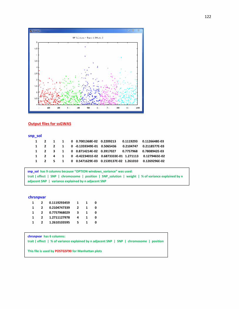
122
Output files for ssGWAS
snp_sol 1 2 1 1 0 0.7001368E-02 0.2209213 0.1119293 0.1126648E-03
1 2 2 1 0 -0.1359349E-01 0.5065436 0.2104747 0.2118577E-03
1 2 3 1 0 0.8714214E-02 0.3917027 0.7757968 0.7808942E-03
1 2 4 1 0 -0.4223401E-02 0.6873333E-01 1.271113 0.1279465E-02
1 2 5 1 0 0.5471629E-03 0.1539137E-02 1.261010 0.1269296E-02
chrsnpvar 1 2 0.1119293459 1 1 0
1 2 0.2104747339 2 1 0
1 2 0.7757968029 3 1 0
1 2 1.2711127978 4 1 0
1 2 1.2610103595 5 1 0
snp_sol has 9 columns because “OPTION windows_variance” was used:
trait | effect | SNP | chromosome | position | SNP_solution | weight | % of variance explained by n
adjacent SNP | variance explained by n adjacent SNP
chrsnpvar has 6 columns:
trait | effect | % of variance explained by n adjacent SNP | SNP | chromosome | position
This file is used by POSTGSF90 for Manhattan plots
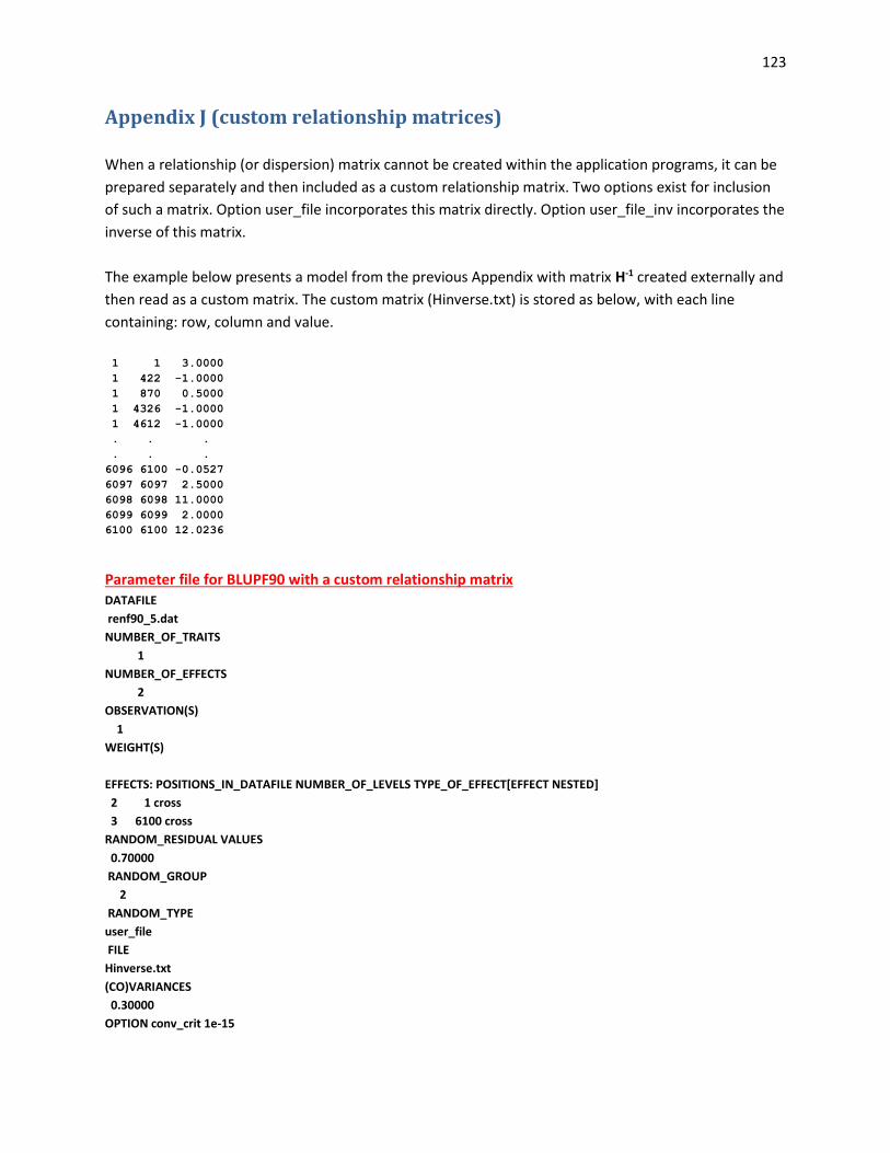
123
Appendix J (custom relationship matrices)
When a relationship (or dispersion) matrix cannot be created within the application programs, it can be
prepared separately and then included as a custom relationship matrix. Two options exist for inclusion
of such a matrix. Option user_file incorporates this matrix directly. Option user_file_inv incorporates the
inverse of this matrix.
The example below presents a model from the previous Appendix with matrix H-1 created externally and
then read as a custom matrix. The custom matrix (Hinverse.txt) is stored as below, with each line
containing: row, column and value.
1 1 3.0000
1 422 -1.0000
1 870 0.5000
1 4326 -1.0000
1 4612 -1.0000
. . .
. . .
6096 6100 -0.0527
6097 6097 2.5000
6098 6098 11.0000
6099 6099 2.0000
6100 6100 12.0236
Parameter file for BLUPF90 with a custom relationship matrix DATAFILE
renf90_5.dat
NUMBER_OF_TRAITS
1
NUMBER_OF_EFFECTS
2
OBSERVATION(S)
1
WEIGHT(S)
EFFECTS: POSITIONS_IN_DATAFILE NUMBER_OF_LEVELS TYPE_OF_EFFECT[EFFECT NESTED]
2 1 cross
3 6100 cross
RANDOM_RESIDUAL VALUES
0.70000
RANDOM_GROUP
2
RANDOM_TYPE
user_file
FILE
Hinverse.txt
(CO)VARIANCES
0.30000
OPTION conv_crit 1e-15

124
Log file for BLUPF90 with a custom relationship matrix name of parameter file?
user.par
* convergence criterion (default=1e-12): 1.0000000E-15
BLUPF90 1.48
Parameter file: user.par
Data file: renf90_5.dat
Number of Traits 1
Number of Effects 2
Position of Observations 1
Position of Weight (1) 0
Value of Missing Trait/Observation 0
EFFECTS
# type position (2) levels [positions for nested]
1 cross-classified 2 1
2 cross-classified 3 6100
Residual (co)variance Matrix
0.70000
Random Effect(s) 2
Type of Random Effect: user defined from file
User File: Hinverse.txt
trait effect (CO)VARIANCES
1 2 0.3000
REMARKS
(1) Weight position 0 means no weights utilized
(2) Effect positions of 0 for some effects and traits means that such
effects are missing for specified traits
Data record length = 3
# equations = 6101
G
0.30000
read 6100 records in 4.7991998E-02 s, 12201 nonzeroes
…
g_usr_inv: read 855620 elements
largest row, column, diagonal: 6100 6100 6100
…
finished peds in 1.776729 s, 861721 nonzeroes
round = 1 convergence = 0.5737E-03
…
round = 80 convergence = 0.9128E-15
80 iterations, convergence criterion= 0.9128E-15
solutions stored in file: "solutions"
The name of custom matrix used is shown here

125
Appendix K (selected programming details)
This section provides some programming insight into an early version of the blupf90 program.
The model is completely described in the module MODEL.
module model
implicit none
! Types of effects
integer,parameter::effcross=0,& !effects can be cross-classified
effcov=1 !or covariables
! Types of random effects
integer, parameter :: g_fixed=1,& ! fixed effect
g_diag=2, & ! diagonal
g_A=3, & ! additive animal
g_A_UPG=4, & ! additive animal with unknown
! parent groups
& g_A_UPG_INB=5, & ! additive animal with unknown
! parent groups and inbreeding
& g_As=6,& ! additive sire
g_PD =7, & ! parental dominance
g_last=8 ! last type
character (40) :: parfile, & !name of parameter file
datafile !name of data set
integer :: ntrait,& !number of traits
neff,& !number of effects
miss=0 !value of missing trait/effect
integer,allocatable :: pos_y(:) !positions of observations
integer :: pos_weight ! position of weight of records; zero if none
integer,allocatable :: pos_eff(:,:),& !positions of effects for each trait
nlev(:),& !number of levels
effecttype(:),& !type of effects
nestedcov(:,:),&!position of nesting effect for each trait
! if the effect is nested covariable
& randomtype(:),& ! status of each effect, as above
randomnumb(:) ! number of consecutive correlated effects
character (40),allocatable:: randomfile(:) ! name of file associated with given
! effect
real, allocatable :: r(:,:),& !residual (co)variance matrix
rinv(:,:),& ! and its inverse
g(:,:,:) ! The random (co)variance matrix for each trait
end module model
The core of the program is presented below.
program BLUPF90
use model;use sparsem; use sparseop
implicit none
real,allocatable :: y(:),& ! observation value
indata(:) ! one line of input data
real :: weight_y ! weight for records
type (sparse_hashm)::xx ! X’X in sparse hash form

126
type (sparse_ija):: xx_ija ! X’X in IJA form, for use with FSPAK only
real, allocatable:: xy(:),sol(:) !X’Y and solutions
real,allocatable :: weight_cov(:,:)
integer,allocatable:: address(:,:) ! start and address of each effect
integer :: neq,io,& ! number of equations and io-status
data_len,& ! length of data record to read
i,j,k,l ! extra variables
real:: val, dat_eff
!
call read_parameters
call print_parameters
neq=ntrait*sum(nlev)
data_len=max(pos_weight,maxval(pos_y),maxval(pos_eff))
print*,'Data record length = ',data_len
allocate (xy(neq), sol(neq),address(neff,ntrait),&
weight_cov(neff,ntrait),y(ntrait),indata(data_len))
call zerom(xx,neq); xy=0
!
call setup_g ! invert R matrices
open(50,file=datafile) !data file
! Contributions from records
do
read(50,*,iostat=io)indata
if (io.ne.0) exit
call decode_record
call find_addresses
call find_rinv
do i=1,neff
do j=1,neff
do k=1,ntrait
do l=1,ntrait
val=weight_cov(i,k)*weight_cov(j,l)*weight_y*rinv(k,l)
call addm(val,address(i,k),address(j,l),xx)
enddo
enddo
enddo
do k=1,ntrait
do l=1,ntrait
xy(address(i,k))=xy(address(i,k))+rinv(k,l)*y(l)*weight_cov(i,k) &
*weight_y
enddo
enddo
enddo
enddo
!
! Random effects' contributions
do i=1,neff
select case (randomtype(i))
case (g_fixed)
continue ! fixed effect, do nothing
case (g_diag)
call add_g_diag(i)
case (g_A, g_As, g_A_UPG,g_A_UPG_INB)
call add_g_add(randomtype(i),i)
case (g_PD)
call add_g_domin(i)
case default
print*,'unimplemented random type',randomtype(i)
endselect
enddo
if (neq < 15) then
print*,'left hand side'
call printm(xx)
print '( '' right hand side:'' ,100f8.1)',xy
endif

127
call solve_iterm(xx,xy,sol)
! Comment the line above and uncomments the lines below only if
! solutions by FSPAK are desired
!xx_ija=xx;
!call fspak90(‘solve’,xx_ija,xy,sol)
if (neq <15) print '( '' solution:'' ,100f7.3)',sol
call store_solutions

128
Modules and Libraries
Module DENSEOP
Subroutines and functions for dense matrix manipulation in Fortran 90.
Uses F90 LAPACK implementation by Alan Miller for some low level routines.
Written by: Tomasz Strabel & Ignacy Misztal, University of Georgia e-mail:
[email protected], [email protected], Oct/5/98-June 8,
2006
The module implements matrix operations on dense general and symmetric matrices. Each
subroutine/function is overloaded to work with several types of arguments. The module is primarily
designed for matrix operations where timing and memory requirements are not critical.
Symmetric matrices
Each of the functions/subroutines works with full-stored and packed (half-stored) matrices. Each
matrix or vector can be single or double precision. However, in one function/subroutine, all
arguments should be of the same precision, and all matrices should be stored the same way.
Subroutines
call chol(a,rank) - Cholesky decomposition
call inverse_s(A,rank)- Generalized inverse: AI = A-
call eigen(A,d,V) - Eigenvalues and eigenvectors: A =V diag(d)*V’
call solve_s(A,b,x) - Generalized solutions: x: Ax=b
The optional variable rank returns the rank of the matrix.
Functions
fchol(A) - Cholesky decomposition
finverse_s(A) - Generalized inverse
fsolve_s(A,b) - Generalized solve
fdet_s(A) - Determinant of A
Procedures for symmetric matrices work with generalized matrices. Redundant rows/columns
equations are determined by operational zero, which is kept in global variable denseop_tol with
default value is 10-10. To change the limit, change the value of the variable in the application
program, e.g., denseop_tol=1d-12
Conversions Let A be a square matrix and AP be a packed matrix
call packit(A,AP) - Conversion from square to packed form; only lower-diagonal
elements are used.

129
call unpackit(AP,A) - Conversion from packed to square form; the matrix is assumed
symmetric.
General matrices
Each matrix or vector can be single or double precision. However, in one function/subroutine, all
arguments should be of the same precision. All matrices are assumed full-rank.
Subroutines
call inverse(A) - Inverse: AI = A-1 call solve(A,b,x) - Solutions: x: Ax=b
Functions
AI=finverse(A) - Returns inverse: AI = Ax=fsolve(A,b) - Computes solutions: x: Ax=b
Printing
call printmat(matrix, text, fmt, un) print any type of matrix using the specified
format fmt and preceded by text. Both text and fmt are optional. If optional un is present, the
output is send to file with unit un.
Warning: The printmat function prints the symmetric packed matrices in full. If a half-stored matrix
is in packed form, it will be printed as full-stored matrix.
Additional subroutines and functions The subroutine(s) and functions below work only with double precision arguments (r8) and
fullstored matrices.
call pos_def(x,text,min_eig,stat) Corrects X if it is not “sufficiently” positive-
definite; ignores rows/columns with 0 elements only.
X - real (r8) symmetric square matrix
text - optional character variable that is printed if X is corrected
min_eig - optional real (r8) variable that sets the minimum relative eigenvalue in X; if
min_eig is missing, 1e-5 is used.
stat - optional logical variable that is set to .true. if X was corrected and .false. if not.
A = diag(b) - creates square diagonal real (r8) matrix with values of real (r8) vector b on
diagonal
b = diag(A) - creates real (r8) vector b containing diagonals of real (r8) matrix A
A=kron(B,C) - A = B “Kronecker product” C; works with real(r4) and real (r8) matrices
Technical details
The basic operations are done in full storage and double precision. Operations with other formats
and precision are obtained by conversions. Computing of eigenvalues/eignevectors and general
matrix operations use parts of LAPACK subroutines as converted by Alan Miller. These subroutines
may contain many more functionality than necessary and may be trimmed to reduce size of the
object code.

130
The modules consist of two files:
lapack90r.f90 - Part of LAPACK denseop.f90 - Interfaces, subroutines, functions and conversion
codes.
For compilation, module kind in file kind.f90 that contains definitions of single and double precision
is also needed.
In the BLUPF90 distribution, these files are included in directory libs and are compiled as denseop.a.
One way to use the denseop module is via a Makefile from an application program in the blupf90
package.
Example (exdense.f90)
Program Example:
use kinds; use denseop
real (r4):: xpacked4(3)=(/1,3,10/) ! Symmetric packed single
precision
real (r4)::x4(2,2) ! Full single precision
real (r8)::x8(2,2) ! Full double precision
call printmat(xpacked4,’ X ‘)
call printmat(fchol(xpacked4),’ Cholesky(X) ‘,’(10(f10.2))')
x4=xpacked4
x8=x4
print*,’ Determinant(xpacked4)=’,fdet_s(xpacked4)
print*,’ Determinant(x8)=’,fdet_s(x8)
print*,’ Determinant(x4)=’,fdet_s(x4)
end
Compilation
To compile standalone:
f90 kind.f90 lapack90r.f90 denseop.f90 exdense.f90
This assumes that all files are in the same directory.
To compile in subdirectory of the blupf90 distribution under Linux/Absoft,
f90 -p ../libs exdense.f90 ../libs/denseop.a
where option -p specifies library directory. This option (-p) is different under different platforms.
See documentation on blupf90 distribution for details.

131
Module SPARSEM
Collection of sparse matrix modules for Fortran 90 useful in animal breeding problems
Written by: Ignacy Misztal, University of Georgia e-mail: [email protected],
9/4/1997 - 5/25/2007
Introduction
Traditionally, programming in animal breeding is done in 2 stages: in a matrix language and in a
regular programming language. Programs in a matrix language such as IML SAS, Matlab,
Mathematica or APL are reasonably simple and useful for creating examples but inefficient for large
problems. Programs in a regular programming language such as Fortran or C/C++ are much more
efficient but could take much longer to write and require substantial training.
Matrix languages are easy to deal with matrices partly because usually only one format is usually
supported: dense rectangular. Operations on such matrices are easy to specify and program, but
large matrices require large memory and long running time. Also, memory and computations are
equal whether matrices are sparse (contain very few nonzero elements) or not. In animal breeding,
many matrices are sparse. If that sparsity is taken into account, the memory requirements and
computations can decrease dramatically. Unfortunately, there is more than one format for storing
sparse matrices, and some computations are fast with one format and but not with another one.
Also, the storage formats and operations are considerably more complicated than dense rectangular
matrices. A library to handle multiple matrix formats and multiple operations would contain many
subroutines, each with a long list of arguments. Such a library would involve considerable learning,
and many details associated with the library would create many opportunities for making a mistake.
One matrix package, Matlab, has some forms of sparse-matrix storage and operations included.
Modern programming languages with “object-oriented” features, such as C++ or Fortran 90, have
abilities to create classes/modules, where many implementation details on specific data structures
can be hidden. A technique called overloading allows single function/subroutine to work with
different formats of its arguments. Therefore, the number of details to remember can be drastically
reduced. Subsequently, programming can be done much easier and quicker.
SPARSEM is a module for Fortran 90 that enables programming common sparse matrix operations
almost as easily as with dense matrices. It supports two dense matrix formats, useful for testing, and
two sparse matrix formats. Changing a program from dense to sparse-matrix format using DENSEM
can be as simple as changing one declaration line. SPARSEM incorporates an interface to FSPAK,
which enables efficient sparse matrix factorization, solving, sparse inversion and calculation of
determinant on matrices much larger than possible with dense matrix structures.

132
Matrix formats
Four matrix formats are available.
DENSEM - dense square matrix.
DENSE_SYMM -dense symmetric upper-stored.
It has approximately only half memory requirements of the dense square matrix.
SPARSE_HASHM - sparse triple accessed by hash algorithm.
This is a very efficient format for set-up and for iterative-solving of sparse matrices.
SPARSE_IJA - Sparse IJA.
This is a memory-efficient format for sparse matrices used by sparse matrix packages.
Format IJA cannot easily be set up directly but can be derived by conversion from the hash
format.
For more information on all these formats see Duff et al, George and Liu, or my class notes.
A popular format that is not included here is linked list. That format is reasonably efficient for
creating and computing with sparse matrices if the number of nonzero elements per row is not too
high and the matrix is not too large. However, the combination of hash plus ija is generally more
efficient.
Matrix operations
The following subroutines/functions are supported. All real scalars and vectors are single precision
unless indicated otherwise.
Operation Description Comments
call init(x) Initialize x Required by standard but usually not necessary because on most systems pointers are initialized automatically
call zerom(x,n) Allocate storage for x as an n*n matrix and zero it
If x was set before, it is reallocated1
call reset(x) Deallocates storage
call addm(a,i,j,x) Add to matrix: x(i,j)=x(i,j)+a
Does not work on SPARSE_IJA
call setm(a,i,j,x) sets element of matrix: x(i,j)=a
Does not work on SPARSE_IJA

133
y=getm(i,j,x) find element of matrix: y=x(I,j)
real(4) function; returns lower-diagonal elements of upper-stored matrix
x=y Conversion between formats
Conversion from sparse to dense formats may require too much storage
call printm(x) Prints x as square matrix
print(x,’internal’) prints sparse matrices in internal format
call solve_iterm(x,rs,sol) Solves: x sol=rs iteratively by SOR
call default_iter (conv,maxround,relax, zerosol)
Changes default iteration parameters
All parameters are optional; default values are: conv(ergence criterion)=1e-10, max round(s)=1000, relax(ation factor)=1.0, zerosol(utions ar beginning of iteration) = .true.
x=block(y,i1,i2,j1,j2) Selects block from y: x=y(i1:i1,j1:j2)
does not work on dense_symm format; may not work with unsymmetric blocks from symmetric matrices
q=quadrf(u,x,v) q=u’Xv real(8) function; does not work on dense_symm format
tr=trace(x,y) Self explanatory real(8) function; x and y must be in same formats; works on densem and sparse_ija formats only
tr=traceblock(x,y,i1,i2,j1, j2)
tr=trace(xy(i1:i2,j1:j 2))
Works as a block-trace combination; produces correct results when blocks of y are nonsymmetric
1The hash matrix is allocated for a default number of elements. If the default is too small, the hash matrix is
enlarged automatically. To change the default p elements, use call zerom(x,n,p). One matrix element in hash
format takes 12 bytes, and for efficient operation there should be at least 10% more nonzero elements
available than used.
All operations assume that the densem type is general while all the other types are upperstored.
Operations tr, quadf work with both upper- and full-stored matrices but the block operation works
literally, i.e., selecting a lower block would return an empty matrix and selecting an upper block

134
would return only an upper-stored matrix. This could be a source of incompatibility between
densem and other formats that use the block operation without taking its limitations into
consideration. Potential problems can be noticed in examples by printing matrices of interest.
Storage type
Matrices in the hash or ija format are half-stored by default. To change the storage type to full, add the option ‘f’ to the addm subroutine: call addm(a,i,j,x,’f’) The subsequent conversion to the ija format will also be full-stored. For conversion from half-stored
hash matrix to full-stored ija, please see a documentation for the GIBBS module.
The printing and other functions/subroutines have been designed for half-stored hash and ija
matrices. Results may not be correct with full-stored matrices.
Numerical accuracy
Module KINDS defines precision r4 to be equivalent to real*4, and r8 to be equivalent to r8.
Precision rh can be set up to r4 or r8 dependent on whether memory or precision is more
important.
Formats DENSEM, DENSE_SYMM, and SPARSE_IJA use precision r8. Format
SPARSE_HASHM uses precision rh. Whenever the precision of numbers in SPARSEM
functions/subroutines is not specified, it is of type rh. Setting rh to r4 is useful when memory usage
needs to be reduced, e.g., for large BLUP programs. Setting rh to r8 is necessary when numerical
accuracy is important, e.g., in variance component programs, and is usually a safer choice.
Diagnostics
Printing of some diagnostic messages depends on the value of an integer variable sparsem_msg.
The value of 3 means maximum diagnostic messages while the value of 0 means no diagnostic
messages. The default is 2. This variable can be set in any part of the application program using the
module SPARSEM.
FSPAK90
FSPAK is a sparse matrix package written in F77 that performs operations on sparse matrices in
format SPARSE_IJA. Operations include solving a system of linear equations by factorization,
calculating a (log)determinant or finding a sparse inverse of a matrix. A sparse inverse is such a
matrix that contains inverse values only for those elements that were nonzero in the original matrix.
For sparse matrices, FSPAK is very efficient computationally.
FSPAK90 is a F90 interface written to simplify the use of FSPAK.
A complete call to FSPAK90 is:
call fspak90(operation,ija,rs,sol,det,msglev,maxmem,rank)
where
operation= “factorize” - calculate sparse factorization

135
“invert” - calculate sparse inverse
“solve” - solve a system of equation
“reset” - reset the storage
“det” - calculate determinant
“stat” - print statistics
“fact_mult” - multiplication by Cholesky factor of the reordered
matrix (if LL=IJA; sol=L*rs)
“inv_fact_mult” - solve the system formed by the Cholesky factor of the
reordered matrix (sol: L*sol=rs)
ija = matrix in SPARSE_IJA form
rs = real (r4) or (r8) vector of right hand side,
sol = real (r4) or (r8), identical to precision of rs, vector of solutions
det = real (r8) determinant or log-determinant
msglev= message level from 0 (minimum) to 3 (maximum); default=0
maxmem=maximum memory available in the system; default=infinite
rank=rank of matrix
All the arguments of fspak90 except “operation” and “ija” are optional except when they are needed
in a specific “operation”. Thus, rs and sol are needed for solving and det for “det” or “ldet”.
Examples: To solve:
call fspak90(’solve’,ija,rs,sol)
for both rs and sol either in single or double precision; all. Preceding steps are done automatically.
To solve using double precision right hand side and solutions: call fspak90(’solve’,ija,rs8=rs,sol8=sol)
To sparse invert: call fspak90(’invert’,ija)
To obtain the determinant d: call fspak90(’det’,ija,det=d)
To obtain the log determinant ld: call fspak90(’ldet’,ija,det=ld)
To obtain rank r with any operation: call fspak90(.....,rank=r)
To force new factorization, when the input matrix has changed: call
fspak90(’factor’,ija)
To deallocate the internal memory:
call fspak90(‘reset’)
To limit memory to a maximum od maxmem, e.g., 20,000k, with any operation call
fspak90(...............,maxmem=20000)

136
Note that only relevant arguments for each step need to be included in calling FSPAK90. Reordering
is performed the first time when FSPAK90 is called. Subsequent factorization except after the option
“reset” will reuse the ordering. Subsequent solves will reuse the factorization.
Additionally:
To sample y from N(0,A) where x~N(0,1) call fspak90(’fact_mult’,A,rs8=x,sol8=y)
To sample y from N(0,A-1) where x~N(0,1) call fspak90(’inv_fact_mult’,A,rs8=x,sol8=y)
For details of the last operations, see Appendix S2
Additional subroutines and functions: Function
y=mult(A,x)
y=mult(x,A)
Implements the matrix by vector multiplication for all matrix formats except dense_symm, and for
double precision x and y.
Subroutine
call multmatscal(A,x)
Implements A=A*x for all matrix formats except dense_symm, and for double precision x.
Hints on using SPARSEM
Initially all the matrices can be implemented in DENSEM format. After the program works well with
an example, convert all data structures for potentially large matrices to sparse formats and verify
that same results are obtained.
Compiling Matrix types and functions subroutine are defined in module sparsem. Subroutine fspak90 is in
module sparseop. Program xx.f90 can be compiled as
f90 -Maa xx.f90 aa/sparsem.a
where aa is the directory containing the modules and the library, and M is the option to include
module directory.
Beginning in May, 1999, SPARSEM is part of a programming package that includes BLUPF90,
REMLF90, GIBSF90 etc. Compilation for several Unix environments is automated by makefiles. To
find details, read Readme and Installation files in the package distributions. To create application
with SPARSEM and possibly other modules, create a subdirectory in the main directory of the
package, and adapt a makefile from the existing directory, e.g., blup.
Sample Programs
Dense matrix solution program

137
program test_sparse_structures
use sparsem; use kinds type
(densem)::x
integer,parameter ::n=5 integer :: i,j
real (rh):: rs(n),sol(n),val
call init(x)
call zerom(x,n)
! set up a sample matrix
do i=1,n
rs(i)=n+1-i
val=10.0*i/i
call addm(val,i,i,x)
do j=i+1,n
val=10.0*i/j call addm(val,i,j,x); call addm(val,j,i,x)
enddo
enddo
print*,'rs: ',rs print*,'matrix' ; call printm(y)
call solve_iterm(y,rs,sol) !solve iteratively print*,'sol: ',sol
end
Triangular dense matrix iterative-solution program ...... type (dense_symm)::x
....... (The rest of the program remains identical)
Sparse hash matrix iterative-solution program
...... type (sparse_hashm)::x
.......
Sparse IJA matrix iterative-solution program
Matrix in ija form cannot be set up directly but can be converted from hash form.
...... type (sparse_hashm)::x
type (sparse_ija)::y
... y=x !conversion
138
call reset(x) ! Optional statement to release storage
print*,'rs: ',rs print*,'matrix' ; call printm(y) call
solve_iterm(y,rs,sol) print*,'sol: ',sol
end
Sparse IJA matrix finite-solution and inversion program with FSPACK90
... use sparsem use sparseop !fspak90 is in module sparseop
..... call fspak90(‘solve’,y,rs,sol)
....
!now invert call
fspak90(‘invert’,y)
call printm(y)
end
References George, A. and Liu, J.W.H. (1981) Computer solution of large sparse positive definite systems.
Prentice-Hall, Englewood Cliffs, N.J.
Appendix S1
Definitions of structure (type)
type densem !traditional dense square matrix
integer :: n
real(8) ,pointer::x(:,:)
end type densem
type dense_symm !upper stored symmetric dense matrix
integer ::n
real(8) ,pointer::x(:)
end type dense_symm
type sparse_hashm
integer:: n,& ! for compatibility mainly
nel,& ! number of elements
filled,& ! number of filled elements
status ! 1 if ready to hash, 2 if in sorted ! order
real (rh) , pointer :: x(:,:)
end type sparse_hashm
type sparse_ija integer :: n,& ! number of equations
nel ! number of nonzeroes

139
integer, pointer::ia(:),ja(:) !will be ia(n+1), ja(m)
real (8), pointer::a(:) !will be a(m)
end type
Accessing structures Structures can be accessed within the application program using the “%” symbol. This is useful, e.g.,
when using Fortran 77 programs. The example below shows how to use a determinant program
written in F77.
type (densem):: z
integer::i,j
real (rh)::value
call init(z)
call zerom(x,2)
! initialize z
do i=1,2
do j=1,2
value=i**j/10. call addm(value, i,j,z)
enddo
enddo
print*, det(z%n,z%x)
end
function det(n,x) !calculate determinant for a 2x2 matrix
integer n
real (r8):: x(n,n),det !
det= x(1,1)*x(2,2)/x(1,2)/x(2,1)
end
Library The following files are compiled into the library:
kind.f90 - definitions of precisions
sparse.f90 - type definitions + main subroutines,
sparse2.f - supporting subroutines (in f77),
fspak.f90 - f90 interface to fspak
fspak.f - main fspak subroutine (in f77),
fspaksub.f - supporting fspak subroutines (in f77),
sparssub.f - low-level subroutines from the book of George and Liu (in f77),
second.f - timing subroutine specific to each computer (in f77).
Subroutines second() specific to other computers can be found in the FSPAK manual.

140
Appendix S2
Multiplication and solving using factors Let A be a matrix. Factorization produced by FSPAK is L:
A=P’LL’P
where P is a reordering matrix chosen to minimize the size of L:
PP’=P'P=I
Operation “fact_mult” multiplies the factor by a vector:
y=P’ L P x
Operation ” inv_fact_mult” solves the system of equation:
P’L’ Py=x
This is equivalent to:
y= P’ (L’-1) Px
Both operations were programmed by Juan Pablo Sanchez. The operations are useful for generation
of large random samples from a multivariate normal distribution. They may be useful in Gibbs
sampler algorithms when setting up and factorization of the system of equations in each round are
feasible.
141
Module Prob Probability routines for use in threshold models and Gibbs sampling
Written by: Ignacy Misztal and Deukhwan Lee, University of Georgia e-mail:
[email protected], 04/29/99-04/19/2001
Module Prob is a collection of random number generators / probabilities / truncated distributions
useful for Gibbs sampling and for threshold models. The module uses features of Fortran 90 to
simplify programnming and high-level optimization to reduce running time, with simplicity being as
important as efficiency. To understand the module fully, please read the documentation on
SPARSEM and on BLUPF90.
Module prob uses high-quality generators from public domain package RANLIB for random number
generators. Some low level code is from Luis Varona.
Subroutines/functions
call set_seed(n)
Sets seed for random number generator to integer n. If this subroutine is not called, the seed will be
selected by the system.
x=gen_uniform(a,b)
a,b - both real (r*) or both integers or both missing.
If a,b are missing, generates samples from uniform(0,1) distribution
If a,b are real (r8), generates samples from uniform(a,b) distribution
If a,b are integers, generates random integer between a and b
x=gen_normal(mean,var)
mean - (r8) scalar or vector
var - (r8) scalar or square matrix
x - (r8) scalar or square matrix
Generates x=N(mean,Var) when mean and var are scalars, or x=MVN(mean,Var) when mean is a
vector and Var is a matrix. Arguments mean and var are optional. If they are missing, sampling is
from N(0,1)
x=gen_invwishart(inv_q_form,df)
inv_q_form - (r8) scalar or square matrix containing inverse of quadratic form
df - an integer containing degrees of freedom
Generates samples from inverted chi square or inverted Wishart distributions.
y=normal(x)
x - real(r8) scalar
y - real (r8) contains density(X) for N(0,1)

142
y=normal_cdf(x)
x - real (r8) scalar
y - real (r8) cumulative distribution function for N(0,1)
y=normal_invcdf(x)
x - real (r8) scalar in the range of <0,1>
y - real (r8) as in: x=normal_cdf(y)
y=generate_trunc_normal(a,b,mean,var)
y - real (r8) scalar or vector
a,b - real (r8) lower and upper bound of random samples
mean - real(r8) scalar or vectors of mean, optional if scalar
var - real(r8) variance or covariance matrix, optional if scalar
If mean and var are missing, generates random samples from N(0,1) distribution truncated to
interval <a,b>.
If mean and var are scalars, generates random samples from N(mean,var) distribution truncated to
interval <a,b>.
If mean is a vector and var is a matrix, generates random samples from MVN(mean,var) distribution
with first dimension truncated to interval <a,b>.
Other functions/subroutines
New functions/subroutines are added to Module prob periodically. Please see program prob.f90 for
details.


![Heritability and breeding value of sheep fertility estimated by ...ptz.icm.edu.pl/download/2009/tom_5_2/3_Piwczynski.pdfof the former, the BLUPF90 computer software [8] was used, and](https://img.pdfslide.us/doc/110x75/612695ba7c5aea54113a1296/heritability-and-breeding-value-of-sheep-fertility-estimated-by-ptzicmedupldownload2009tom523.jpg)


![SOFTWARE Open Access GVCBLUP: a computer package for … · 2017. 8. 25. · DMU [13], BLUPF90 [14]). User-friendliness of the com-puting tool affects the efficiency of data analysis](https://img.pdfslide.us/doc/110x75/6126989f68aa2d4fb230ee3f/software-open-access-gvcblup-a-computer-package-for-2017-8-25-dmu-13-blupf90.jpg)