Vassar CollegeDigital Window @ Vassar

Senior Capstone Projects

2013

Manual and landmark-based morphometriccomparison of two populations of Campeloma, sp.across the K-Pg boundaryGary D. Linkevich

Follow this and additional works at: http://digitalwindow.vassar.edu/senior_capstone

This Open Access is brought to you for free and open access by Digital Window @ Vassar. It has been accepted for inclusion in Senior CapstoneProjects by an authorized administrator of Digital Window @ Vassar. For more information, please contact library_thesis@vassar.edu.

Recommended CitationLinkevich, Gary D., "Manual and landmark-based morphometric comparison of two populations of Campeloma, sp. across the K-Pgboundary" (2013). Senior Capstone Projects. 236.http://digitalwindow.vassar.edu/senior_capstone/236

Manual and landmark-based morphometric

comparison of two populations of Campeloma, sp.

across the K-Pg boundary

Gary D. Linkevich Dept. of Earth Science and Geography

May 2013

Submitted to the faculty in partial fulfillment of the requirements for the degree of Bachelor of Arts in Earth Science

Vassar College, Poughkeepsie, New York, 12604

Thesis Advisors: Stephanie L. Peek, David P. Gillikin, David H. Goodwin

TABLE OF CONTENTS

Abstract .................................................................................................................................................... 1 Acknowledgments .................................................................................................................................. 2 List of Figures ......................................................................................................................................... 3 List of Tables ........................................................................................................................................... 3 CHAPTER 1: INTRODUCTION 1.1 Scientific Context ...................................................................................................................... 4 1.2 Geological Context ................................................................................................................... 5 1.3 Study Setting .............................................................................................................................. 6 CHAPTER 2: METHODS 2.1 Sample Collection ..................................................................................................................... 8 2.2 Manual Morphometrics ........................................................................................................... 12 2.3 Landmark Morphometrics ...................................................................................................... 12 2.3.1 Data Acquisition ................................................................................................................... 12 2.3.2 Data Optimization ............................................................................................................... 15 2.3.3 Skew ....................................................................................................................................... 16 2.3.4 Components of Variation ................................................................................................... 17

2.4 X-Ray Diffraction ..................................................................................................................... 18 2.5 Stable Isotope Analysis ............................................................................................................ 19 CHAPTER 3: RESULTS 3.1 X-Ray Diffraction ..................................................................................................................... 20 3.2 Stable Isotopes .......................................................................................................................... 21 3.3 Manual Morphometrics ........................................................................................................... 22 3.4 Landmark Morphometrics ...................................................................................................... 22 CHAPTER 4: DISCUSSION 4.1 XRD and Stable Isotope Analysis........................................................................................... 26 4.2 Manual Morphometrics ........................................................................................................... 27 4.3 Landmark Morphometrics ...................................................................................................... 29 4.4 Considerations ........................................................................................................................... 30 CHAPTER 5: CONCLUSION 5.1 Summary of Results .................................................................................................................. 31 5.2 Suggestions for Future Work .................................................................................................. 31 REFERENCES ................................................................................................................................... 33 APPENDIX: XRD RESULTS ......................................................................................................... 35

1

ABSTRACT

Understanding how species survive mass extinction events allows scientists to more fully

explore the effects of major biotic change in the fossil record. The Cretaceous-Paleogene (K-

Pg) extinction 65.5 Ma was one of the largest extinction events in Earth’s history and profoundly

affected both terrestrial and marine life. Fossiliferous exposures of the Hell Creek and Fort

Union Formations in the northern Great Plains of the western U.S. offer some of the best

available records of conditions before and after the K-Pg boundary. Similarly, due to their hard

aragonitic shells, conispiral geometry, and prevalence throughout the Phanerozoic Eon, well-

preserved gastropods (snails) are perfect candidates for morphometric and stable-isotope

analyses aimed at reconstructing paleoecological information.

In this study, I compared two populations of the freshwater gastropod Campeloma sp.,

one from before and from after the K-Pg boundary at Hell Creek, Montana. I used principal

components analysis (PCA) of 6 manually measured and 10 landmark-based components of

shell morphological variation to compare the two populations, in order to investigate any

possible anatomical differences that may have arisen in response to the extinction event.

Likewise, I used stable oxygen isotope analysis to investigate potential differences in ontogeny or

growth rate. Taken together, the stable isotope and morphometric analyses suggest that

Campeloma sp. exhibited no major ontogenetic or anatomical differences in response to the events

that triggered the K-Pg extinction. This suggests that Campeloma was capable of withstanding

dramatic environmental change with little to no adaptation in shell morphology.

2

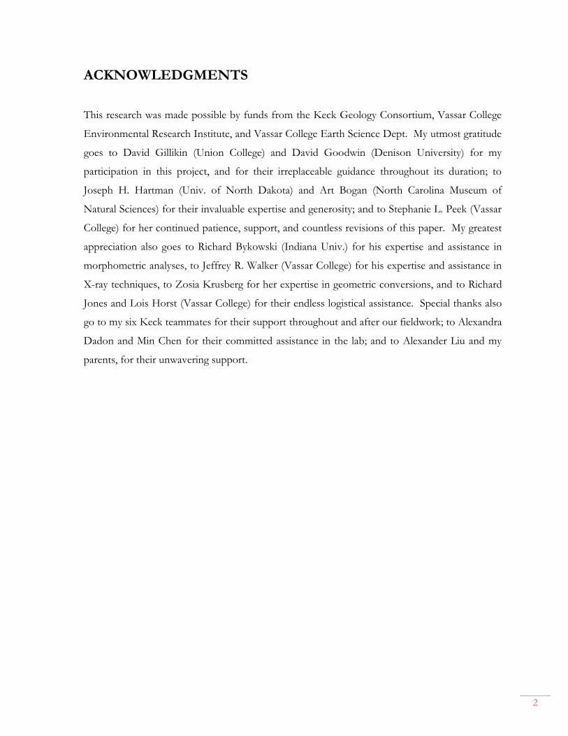
ACKNOWLEDGMENTS

This research was made possible by funds from the Keck Geology Consortium, Vassar College

Environmental Research Institute, and Vassar College Earth Science Dept. My utmost gratitude

goes to David Gillikin (Union College) and David Goodwin (Denison University) for my

participation in this project, and for their irreplaceable guidance throughout its duration; to

Joseph H. Hartman (Univ. of North Dakota) and Art Bogan (North Carolina Museum of

Natural Sciences) for their invaluable expertise and generosity; and to Stephanie L. Peek (Vassar

College) for her continued patience, support, and countless revisions of this paper. My greatest

appreciation also goes to Richard Bykowski (Indiana Univ.) for his expertise and assistance in

morphometric analyses, to Jeffrey R. Walker (Vassar College) for his expertise and assistance in

X-ray techniques, to Zosia Krusberg for her expertise in geometric conversions, and to Richard

Jones and Lois Horst (Vassar College) for their endless logistical assistance. Special thanks also

go to my six Keck teammates for their support throughout and after our fieldwork; to Alexandra

Dadon and Min Chen for their committed assistance in the lab; and to Alexander Liu and my

parents, for their unwavering support.

3

LIST OF FIGURES

1. Biological diversity throughout the Phanerozoic Eon, with the K-Pg event indicated. 2. (a) Map of Great Plains, indicating exposures of Fort Union and Hell Creek formations.

(b) Stratigraphic cross section from Hell Creek, MT, to Huff, ND 3. Map of the Fort Peck Lake East quadrangle, with locations of collection sites described. 4. Comparison of the fossil assortment collected at the two localities visited. 5. Comparison of the sediments at the two localities visited. 6. Setup used to photograph the specimens used in this study. 7. A map of the landmarks used in this study, with landmark definitions included. 8. Visual representation of the optimization process used to streamline the landmark data. 9. A diagram of the influence of skew upon linear measurements. 10. A photograph of one of the Paleogene specimens sampled for stable isotope analysis. 11. Frequency distributions of observed offset in XRD dValues. 12. Stable oxygen isotopic curves for the four gastropods analyzed. 13. Principal components analysis of manually obtained morphometric data. 14. Principal components analysis of landmark-based morphometric data. 15. Principal components analysis of landmark-based morphometric data, with Δθ removed. 16. Scans of two specimens from each population cut in half along the vertical axis.

LIST OF TABLES

1. Comparison of the parameters of variation obtained from the two morphometric methods.

4

CHAPTER 1: INTRODUCTION

1.1 SCIENTIFIC CONTEXT

In the three decades since Alvarez et al. (1980) published crucial evidence for a bolide

impact as the primary cause of the Cretaceous-Paleogene (K-Pg) extinction, the focus of

research regarding this cataclysmic event has slowly shifted away from debating its probable

causes and towards exploring its environmental and biotic consequences. Some of the best

records of these conditions are available in the Mesozoic and early Cenozoic sediments of the

western United States, particularly the late-Cretaceous Hell Creek and early-Paleogene Fort

Union Formations. Similarly-motivated studies of these strata have explored a wide range of

available information, from sedimentology to paleobotany. The richness and concentration of

fossil beds in these formations also allows for anatomically-driven studies in morphometrics and

population statistics.

Gastropods (snails) have been the subject of numerous morphometric studies over the

past few decades due to their taxonomic diversity, consistent presence throughout the

Phanerozoic, and excellent preservation potential. Much of this research has been dedicated to

quantifying and systematizing morphometric analysis. Kohn and Riggs (1975) analyzed linear

measurements of specimens and photographs to characterize shells of the marine gastropod

Conus, and noted the need for precise, objective methods when selecting, coding, and evaluating

character states. As technological advances offered newer ways of obtaining and handling data,

landmark-based geometric morphometric analyses became possible and quickly surpassed

manual morphometrics in popularity among gastropod studies (Vuolo et al., 2011).

The goal of this study is to explore potential changes in the anatomy and lifestyle of the

freshwater gastropod Campeloma sp. that may have arisen as a result of the K-Pg extinction event.

5

I investigated this issue using morphometric analyses (both manual linear measurements and

landmark-based geometry) and geochemical analyses (stable isotopes and X-ray diffraction) of

two populations of Campeloma, one from before and one from after the K-Pg boundary.

1.2 GEOLOGICAL CONTEXT

The K-Pg extinction (formerly known as the “K-T,” T standing for Tertiary, an obsolete

term for the period of time spanned by the Paleogene and Neogene) was the most recent of the

“Big Five” mass extinction events in the Phanerozoic (Fig. 1) (Butterfield, 2007). While

opinions regarding the number of mass extinctions in history vary depending on the standards

used for extinction rate, the bar is usually set at 50% of all animal species (Butterfield, 2007).

The K-Pg boundary suits this criterion easily, given that it witnessed the loss of about 17% of all

families, 50% of all genera, and 75% of all species (Jablonski, 1994). While the magnitude of the

event’s consequences for terrestrial animals is notorious given the demise of the non-avian

dinosaurs, the consequences for

marine biota are not to be

overlooked. Within the

mollusks, for instance, the

number of cephalopod and

bivalve genera was diminished

severely (Macleod et al., 1997); in

fact, apart from nautiloids and

coleoids, all cephalopods went

extinct (Harries et al., 2002).

Figure 1. Biological diversity on the familial level throughout the Phanerozoic Eon, with the 5 major extinction events indicated: (1) Late Ordovician, (2) Late Devonian, (3) Permian-Triassic, (4) Triassic-Jurassic, (5) Cretaceous-Tertiary (Paleogene). http://jpkc.nwu.edu.cn/dqswx/Figures/Figure%207.21.jpg

6

1.3 STUDY SETTING

The Hell Creek Formation (Fm.) is consistently underlain by the Fox Hills Fm. and

overlain by the Fort Union Fm. throughout the Williston Basin (Fig. 2a), although given the

basin’s longitudinal extent, different members of these formations make the contact throughout

the area. For instance, the Colgate Member (Mbr.) of the Fox Hills Fm. that underlies the Hell

Creek Fm. in the west pinches out stratigraphically by North Dakota, and the Tullock Mbr. of

the Fort Union Fm. in the west is replaced by the Ludlow Mbr. inter-fingering with the marine

Cannonball Mbr. from the east (Fig. 2b) (Johnson et al., 2002). As the Hell Creek Fm. and Fort

Union Fm. were deposited in primarily freshwater environments, this inter-fingering represents

the last known transgression-regression cycle of the Western Interior Seaway in North America

(Hartman 2002). Given that both sampling locations for this study were in or near the Fort

Peck reservoir at the western edge of the Williston Basin (Fig. 2a), the stratigraphic context for

the study is the progression from the Hell Creek Fm. to the Tullock Mbr.

Wilde and Bergantino (2004) described the Hell Creek Fm. as a 100-150 m-thick

combination of gray to grayish-brown, fine to medium-grained sandstone and smectitic, silty

shale. Sediments of the Hell Creek Fm. also include carbonate concretions amongst the finer

sandstone and occasional popcorn weathering in the shale. While largely similar in texture, the

sandstone beds that comprise most of the Tullock Mbr. (80-90 m thick) are yellowish-gray in

color, exhibit a broad range of massive, planar, and trough cross bedding, and tend to be more

thin, tabular, and laterally persistent. The Tullock sandstone is also interbedded with brownish-

to purplish-gray claystones and carbonaceous shales. Sediments of both the Hell Creek Fm. and

Tullock Mbr. are generally poorly cemented, prone to weathering, and occasionally interbedded

by thin, somewhat lenticular coal beds.

7

Figure 2. (a) Map of northern Great Plains indicating exposures of Fort Union, Hell Creek, and associated formations. Geographic context for this study outlined in orange. Note Fort Peck Reservoir near Hell Creek (HC), shown in greater detail in Fig. 3. Line of cross-section for (b) indicated in red. From Figure 1 (Johnson et al., 2002). (b) Stratigraphic cross section from Hell Creek, MT, to Huff, ND, showing thickness of Hell Creek and adjacent strata. From Figure 2 (Johnson et al. 2002).

8

CHAPTER 2: METHODS

2.1 SAMPLE COLLECTION

I collected all specimens around the Fort Peck Reservoir on the western edge of the

Williston Basin, Montana (Fig. 3), on July 14-15, 2012. I obtained the Cretaceous specimens

from a fossil-rich (Fig. 4a) exposure of the Hell Creek Formation at Hartman site L6867 (N 47°

45' 10.8", W 106° 29' 56.4”, elev. 784 m). Most Cretaceous specimens were selected from float

(Fig. 5a), although some were extracted from a large consolidated block that had recently rolled

down from the conglomerated shell-bearing layer, and a few were collected in situ. I obtained

Paleogene specimens from a series of broad promontories composed of much less fossiliferous

(Fig. 4b) unconsolidated mudstone and sporadic red sandstone, representing the Tullock

member of the Paleogene Fort Union Formation, at Hartman site L6978 (N 47° 18' 43.2”, W

106° 46' 8.4", elev. 798 m). Paleogene specimens were collected in situ (Fig. 5b).

9

Figure 3. A closer look at the Fort Peck Lake East 30’ x 60’ quadrangle. The location of the Cretaceous (HC) sampling site is designated by point K; the Paleogene sampling site is slightly outside (to the south) of the inset’s field of view. For spatial context, see Fig. 2a. From Figure 1 (Wilde and Bergantino, 2004).

10

Figure 4. Comparison of the fossil assortment collected at the two localities visited. (a) A small, random sample of the numerous Cretaceous specimens collected. (b) The full set of Paleogene specimens collected.

11

Figure 5. Comparison of the sediments at the two localities visited. Note the richly fossiliferous, mostly lithified matrix at the Cretaceous site (a), compared to the looser, fossil-poor sediments of the Paleogene site (b).

12

2.2 MANUAL MORPHOMETRICS

The initial stage of data acquisition for this study relied on manual measurements. All 53

originally collected Paleogene specimens, and a small selection of the Cretaceous specimens,

were measured with a caliper (to the nearest 0.1 mm) and goniometer (to the nearest integer). I

used a caliper to obtain overall height, maximum major and minor diameters, last whorl height,

and ‘modified aperture height’ (MAH), defined as the height from the bottom of the shell to the

shoulder immediately above the aperture (landmark 5 in Fig. 7). I used a goniometer exclusively

to find the low-whorl angle (LWA; defined as the angle formed by the intersection of the lines

tangent to either side of the shell’s spire at the last 2 whorls). I then utilized some of these

measurements to determine compound parameters, including maximum cross-sectional area

(MXSA) and cross-sectional ellipticity (XSE). MXSA is an effective indicator of overall shell

size, while XSE captures a combination of fossil deformation and terminal aperture growth rate,

since the end-of-life value of the rate at which the width of the aperture increases throughout

the shell determines how extreme the aperture width / shell width ratio becomes. I analyzed all

of the manual morphometric data using the paleontological statistical software package PAST

(Hammer & Harper 2001).

2.3 LANDMARK MORPHOMETRICS

2.3.1 Data Acquisition

For the landmark-based component of this study, I photographed all 622 specimens

using a Canon XSi digital camera and 28-135mm Ultrasonic lens. I kept photographs consistent

by using modeling clay to hold each specimen in the same position, a spotlight to provide steady

lighting, and a tripod and external remote to minimize camera movement and vibration (Fig. 6).

13

Figure 6. Setup used to photograph the specimens used in this study. Photograph by Min Chen (Vassar College).

I evaluated the photographs based on four parameters: presence of an intact bottom

edge, visibility of the aperture, presence of a leading aperture edge, and presence of a complete

apex. Most specimens failed in one or two of these criteria, but 141 of them failed in all four

due to their poor preservation; these specimens I discarded. I digitized the remaining

photographs using the TPS software suite (Rohlf 2005). Grouping photos by the

aforementioned criteria made it possible to take advantage of well-preserved specimens while

plotting only clear points on more weathered specimens, thereby maximizing the amount of

robust data obtained and minimizing any estimation.

I placed landmarks at some combination of 15 generally well-preserved locations on

each specimen, as shown in Figure 7. I omitted some landmarks for some specimens only if

they lacked the physical features to allow for such landmark placement. Landmark locations

14

were chosen after consideration of consistently preserved shell features as well as landmarks

utilized by numerous other studies (Kohn and Riggs, 1975; Chiu et al., 2002; Cruz et al., 2011;

and Queiroga et al., 2011; to name a few).

Figure 7. Landmarks used in this study, plotted on a well-preserved Cretaceous specimen. Definitions for the landmark locations are: 1) Bottom edge of shell; 2) Innermost edge of aperture; 3) Outermost edge of aperture; 4) Uppermost edge of aperture; 5) Joint between the shoulder above the aperture and the wall of the last whorl; 6-15) Further joints between each whorl and the shoulder of the next whorl, with the exception of: 10) Furthest-left point on the shell when the central axis is positioned vertically; and 13) Apex.

15

2.3.2 Data Optimization

I then optimized the cumulative data obtained to create the best possible database of

complete information. None of the Paleogene specimens had intact apices, so for comparative

purposes, I discarded apex data from the Cretaceous specimens. Marginal specimens and those

with limited sets of data I likewise disregarded for the sake of robust statistical comparison (this

included Paleogene specimens with only low-whorl data, Paleogene specimens with only low-

whorl and bottom data, and Cretaceous specimens without bottom data). This produced a final

sample population of 30 Paleogene and 128 Cretaceous specimens (Fig. 8).

Figure 8. Visual representation of landmark data obtained from all specimens, created by visually condensing and rotating (90° counterclockwise) the rows and columns of values in the Microsoft Excel spreadsheet containing the data. Data from Paleogene specimens are highlighted in blue; all other data come from Cretaceous specimens. Blanks indicate missing data (data that could not be collected from a particular specimen). (a) Cumulative initial data; (b) Total data after the removal of apex data, marginal Paleogene specimens, and morphometrically poor Cretaceous specimens; (c) Final data used for all statistical comparisons.

16

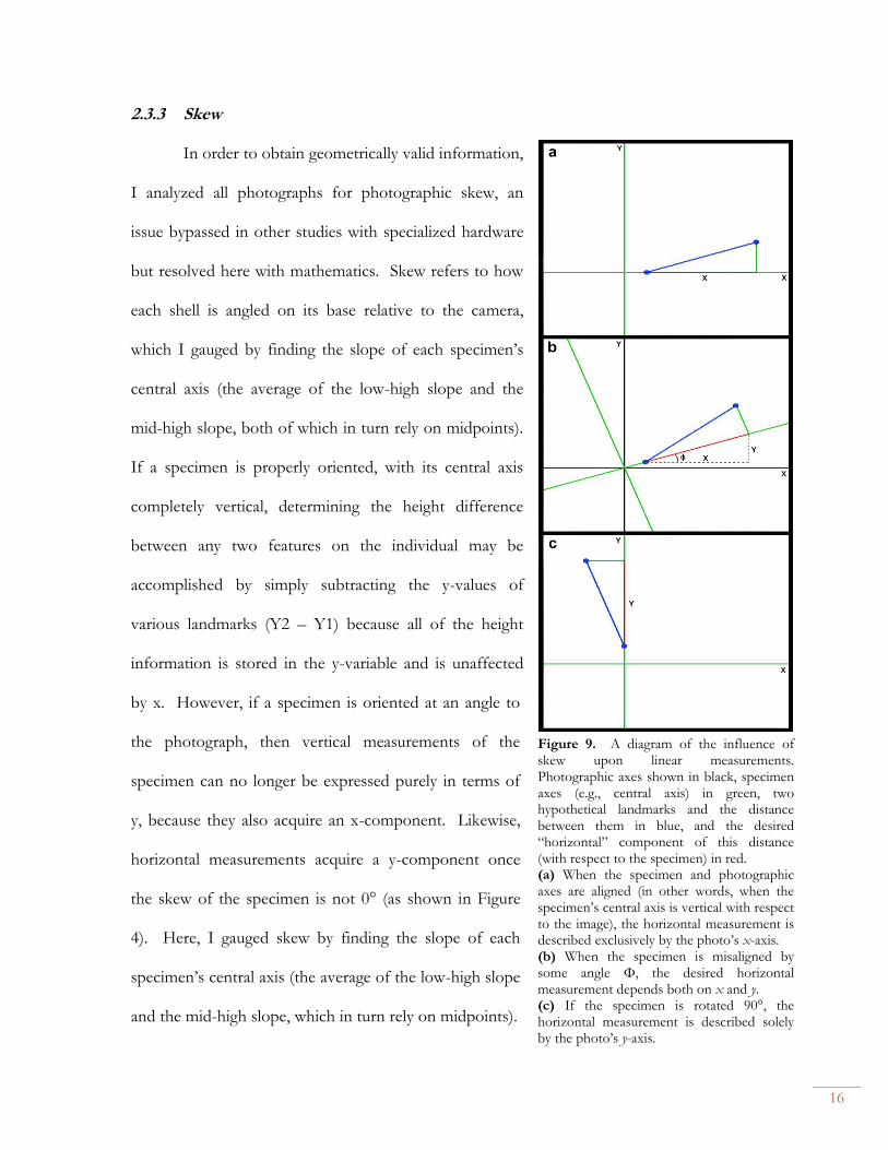
2.3.3 Skew

In order to obtain geometrically valid information,

I analyzed all photographs for photographic skew, an

issue bypassed in other studies with specialized hardware

but resolved here with mathematics. Skew refers to how

each shell is angled on its base relative to the camera,

which I gauged by finding the slope of each specimen’s

central axis (the average of the low-high slope and the

mid-high slope, both of which in turn rely on midpoints).

If a specimen is properly oriented, with its central axis

completely vertical, determining the height difference

between any two features on the individual may be

accomplished by simply subtracting the y-values of

various landmarks (Y2 – Y1) because all of the height

information is stored in the y-variable and is unaffected

by x. However, if a specimen is oriented at an angle to

the photograph, then vertical measurements of the

specimen can no longer be expressed purely in terms of

y, because they also acquire an x-component. Likewise,

horizontal measurements acquire a y-component once

the skew of the specimen is not 0° (as shown in Figure

4). Here, I gauged skew by finding the slope of each

specimen’s central axis (the average of the low-high slope

and the mid-high slope, which in turn rely on midpoints).

Figure 9. A diagram of the influence of skew upon linear measurements. Photographic axes shown in black, specimen axes (e.g., central axis) in green, two hypothetical landmarks and the distance between them in blue, and the desired “horizontal” component of this distance (with respect to the specimen) in red. (a) When the specimen and photographic axes are aligned (in other words, when the specimen’s central axis is vertical with respect to the image), the horizontal measurement is described exclusively by the photo’s x-axis. (b) When the specimen is misaligned by some angle Φ, the desired horizontal measurement depends both on x and y. (c) If the specimen is rotated 90°, the horizontal measurement is described solely by the photo’s y-axis.

17

2.3.4 Components of Variation

I used various measurements derived from the landmark data to establish ten parameters

of variation. These are described below, and compared to the parameters obtained from the

manual morphometric data in Table 1:

1. Aperture area, approximated using landmarks 1-4 to establish semimajor and semiminor

elliptical diameters;

2. Aperture elongation, the ratio between aperture height and width, with values > 1

signifying a taller (rather than wider) ellipse;

3. Shell width, the horizontal distance between landmarks 3 and 10;

4. Ratio of aperture width to shell width;

5. Height of the last whorl, the vertical distance between landmarks 1 and 6;

6. Height of the last 2 whorls, the vertical distance between landmarks 1 and 7;

7. Ratio of parameters 5 and 6;

8. θ low , the angle formed at the intersection of the two slopes between the last and

previous-to-last whorl on either side (synonymous to LWA in the manual

measurements);

9. θ mid , synonymous to θ low , but using the next 2 whorls;

10. Δθ, defined as the difference between parameters 8 and 9.

For principal components analysis, I log-corrected parameters 8-10 to minimize the

difference in magnitude of discrepancies, compared to parameters 1-7.

18

Table 1. Comparison of the parameters of variation obtained from the two morphometric methods, sorted by type. Juxtaposition on the same row indicates synonymy.

Parameter Type Manual Landmark

Total Height Height Height

Last Whorl

Last Whorl Last Whorl

- Last 2 Whorls

- Last 1 / Last 2

Aperture

Mod. Aperture Height -

- Aperture Area

- Aperture Elongation

Diameter

Minor Diameter -

Major Diameter Shell Width

- Aperture Width / Shell Width

Cross-Sectional Max Cross-Sect. Area (MXSA) -

Cross-Sect. Ellipticity (XSE) -

Angular

Low-whorl angle (LWA) θ low

- θ mid

- Δθ

2.4 X-RAY DIFFRACTION

Using a Dremel rotary drill equipped with a diamond-coated bit, I sampled two

specimens from each population and analyzed the resulting powders from 15° to 45° inclination

with a Bruker D2 Phaser desktop diffractometer at Vassar College, Poughkeepsie, NY. The

results were processed in the Bruker DIFFRAC software suite. Due to concerns regarding

potential shell/matrix sampling cross-contamination, I also separately sampled the shell and

matrix of one specimen from each group. I ensured that one of the specimens I chose from

each group was also one of the two I had earlier chosen from each population for stable isotope

analysis.

19

2.5 STABLE ISOTOPE ANALYSIS

I selected two well-preserved specimens from each group for stable isotope analysis,

cleaned with a brush to remove excess matrix, and sampled at 20 locations per shell. These

locations were approximately regular with respect to linear, non-curved distance, corresponding

to the animal’s growth. However, given the shell’s increasing diameter (and likewise,

circumference), this translated to an increase in the number of samples per whorl from apex to

aperture (Fig. 10). I took all samples on the whorl, from apex to aperture, with an NSK Volvere

V-max drill equipped with a 300-micron bit.

δ18O values of aragonite from the 80 samples were measured at the Environmental

Isotope Laboratory at the

Department of Geosciences,

University of Arizona, using an

automated carbonate preparation

device (KIEL-III) coupled to a

gas-ratio mass spectrometer

(Finnigan MAT 252). Powdered

samples were reacted with

dehydrated phosphoric acid under

vacuum at 70°C. The isotope

ratio measurement was calibrated

based on repeated measurements

of NBS-19 and NBS-18, and

precision is ± 0.1 ‰ for δ18O (1σ).

Figure 10. A photograph of one of the Paleogene specimens sampled for stable isotope analysis, showing the drill holes from sampling.

20

CHAPTER 3: RESULTS

3.1 X-RAY DIFFRACTION

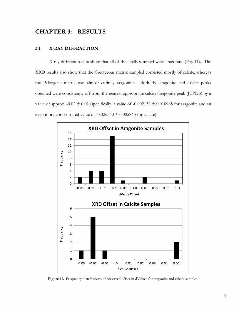
X-ray diffraction data show that all of the shells sampled were aragonitic (Fig. 11). The

XRD results also show that the Cretaceous matrix sampled consisted mostly of calcite, whereas

the Paleogene matrix was almost entirely aragonitic. Both the aragonite and calcite peaks

obtained were consistently off from the nearest appropriate calcite/aragonite peak (JCPDS) by a

value of approx. -0.02 ± 0.01 (specifically, a value of -0.002132 ± 0.010985 for aragonite and an

even more concentrated value of -0.026340 ± 0.005843 for calcite).

Figure 11. Frequency distributions of observed offset in dValues for aragonite and calcite samples.

21

3.2 STABLE ISOTOPE ANALYSIS

Stable isotopic data for the four specimens analyzed yielded distinct but unclear trends

(Fig 12). The curve of δ18O values exhibited irregular but periodic fluctuations, generally

increasing in magnitude from apex to aperture, for both Cretaceous shells and one of the

Paleogene specimens. For the remaining Paleogene shell, fluctuation was small enough that the

trend could almost be called linear, with the exception of one large spike near the aperture. The

δ18O values had averages of -10.62‰ ± 0.49‰ and -11.36‰ ± 0.66‰ for the two Cretaceous

shells, and averages of -10.42‰ ± 0.58‰ and -10.35‰ ± 0.32‰ for the two Paleogene shells.

Figure 12. δ18O curves for the 4 samples analyzed. Color has been added purely to distinguish the

two individuals in each pair, and has no other significance.

22

3.3 MANUAL MORPHOMETRICS

A principal components analysis (PCA) of manually obtained linear data showed a high

degree of separation between the two groups of specimens, with only a small amount of overlap

(Fig. 13a). PC1 consisted of a strong positive correlation between shell height and MXSA, as

well as a weaker positive correlation between MAH and last whorl height. XSE and log(LWA)

are statistically irrelevant (Fig. 13b). PC2 was overall very similar to PC1, with the exception that

MXSA was negatively correlated with the axis, and log(LWA) contributed slightly more than in

PC1 (Fig. 13c).

3.4 LANDMARK MORPHOMETRICS

I ran principal component analysis twice for the landmark-based data – once with log

(Δθ) and once without – because angular measurements were much more difficult to acquire

than linear measurements, and the compound angular parameter log (Δθ) was therefore prone to

error and inconsistency (this will be discussed in further detail later). Overall, landmark-obtained

morphometric data showed far less separation between the two groups than did the manual

results, with most of the data in overlap (Fig. 14a; 15a). In both runs, PC1 consisted of a

positive correlation with aperture area, shell width, and the height of the last 1 and last 2 whorls;

a very weak negative correlation with aperture elongation, log(θ low), and log(θ mid); and almost no

contribution from the aperture/shell width ratio or last 1 / last 2 whorl ratio (Fig. 14b, 15b). In

the first run, PC2 was almost entirely controlled by a positive correlation with log(Δθ), with little

and mostly negative influence from all other parameters; in the second run, PC2 was mostly

comprised of a strong positive correlation with aperture elongation and a negative correlation

with the aperture/shell width ratio.

23

Figure 13. Principal components analysis of manually obtained morphometric data. (a) Scatter plot. (b) Loadings for PC1 (horizontal). (c) Loadings for PC2 (vertical). All figures created in PAST and edited in Adobe Photoshop.

24

Figure 14. Principal components analysis of landmark-based morphometric data. (a) Scatter plot. (b) Loadings for PC1 (horizontal). (c) Loadings for PC2 (vertical). All figures created in PAST and edited in Adobe Photoshop.

25

Figure 15. Principal components analysis of landmark-based morphometric data, with Δθ removed. (a) Scatter

plot. (b) Loadings for PC1 (horizontal). (c) Loadings for PC2 (vertical). All figures created in PAST and edited in Adobe Photoshop.

26

CHAPTER 4: DISCUSSION

4.1 XRD AND STABLE ISOTOPE ANALYSIS

X-ray diffraction results confirm that all sampled specimens are aragonitic, which

(considering the instability of aragonite) rules out the possibility of diagenetic alteration

influencing the isotopic values. The observed offset (-0.02 ± 0.01 in dValue) in XRD data is

most likely due to instrumental error. Given the diffractometer’s very recent installation at its

facility, the observed consistent offset of mineral data peaks from their expected values suggests

a potential error in the instrument’s calibration, or alternatively, a possible error in sampling and

mounting style (with the former the likelier possibility). Based on its small standard deviation,

the error was mostly removed with a simple adjustment of data (+0.02 dValue). Therefore, all

variations in the data are due to physiological and/or environmental factors. In particular, the

primary controlling agent of δ18O values is seasonal temperature fluctuation, which therefore

makes them suitable for investigations of ontogenetic age.

A preliminary exploration of stable isotope data highlighted the notable variability of the

δ18O value curves. The cause of this irregularity has yet to be determined, but a greater number

of samples from each shell would undeniably offer a more complete representation of actual

values. As it stands, the possibility of omitted (or perhaps even misleading) peaks is non-

negligible. However, assuming the available data accurately depict true trends, the ontogenetic

ages of both Cretaceous specimens, as well as the “regular” Paleogene individual, are best

estimated at 4-6 years. A similar estimation cannot be made for the anomalous Paleogene

specimen due to the lack of evident spikes in its data (Fig. 12). The importance of the single

spike in this specimen’s δ18O values is not clear.

27

XRD results show that the matrices of the two shell groups differ in composition, which

corresponds well to the difference in matrix texture. Together with the poor preservation state

of most of the Paleogene specimens, this suggests that the Paleogene sediment is composed

largely of eroded shell material. This makes sense, given the poorly preserved, eroded state of

the Paleogene specimens collected (Fig. 4b.).

4.2 MANUAL MORPHOMETRICS

The four parameters comprising PC1 (height, MXSA, aperture height, and last whorl)

(Fig. 13b) are all fundamentally synonymous to the organism’s overall age and size. Their

mutual positive correlation supports the basic notion that all of them increase steadily over the

course of the organism’s lifespan, as well as the additional notion that all of the information they

represent could therefore be represented by any one of them. This is corroborated by the

findings of McShane et al. (1994), who concluded that shell height alone among 61 populations

of abalone (Haliotis iris) captured over 70% over the variation in other parameters covarying with

specimen length. In Fig. 14, it is fairly obvious that PC1 shows a strong difference between the

two populations, and seems to imply that Cretaceous shells were generally much larger than their

Paleogene counterparts. While this is technically true, it cannot be interpreted as a robust

anatomical or ontogenetic difference between the two populations due to a twofold

preservational and sampling bias.

First, as shown in Fig. 5, the contrast in depositional environment is striking, and this

has implications not only for the number of specimens preserved (and thus, collected), but also

for the state of preservation seen in the two populations (see Fig. 16). The magnitude of this

difference is such that a great number of Cretaceous individuals had to be disregarded because

their apex data were of no use without Paleogene apex data for comparison (Fig. 8).

28

Second, due to the fact that the

Cretaceous locality was explored the day before

the Paleogene, as well as to human

overexcitement, the specimens collected at the

Cretaceous site were the biggest and best-

preserved; that is, almost no juveniles were

collected (Fig. 4a). In other words, an attempt to

collect as much morphometric data as possible in

fact resulted in a significant gap, and created an

unrepresentative sample of the locality. By

contrast, fossil density at the Paleogene locality

was so low that I had to collect any and all

specimens I found, creating a representative

sample of locality and including both adults and

juveniles (Fig. 4b).

PC 2 demonstrates a strong negative

(inverse) correlation between MXSA the other

three size-related parameters, suggesting that some individuals are more bulbous (that is, with

greater MXSA given a smaller height) while others are more slender (smaller MXSA given a

greater height). This difference is not due to preservational deformation, because XSE

(ellipticity) is a non-factor in both principal components; that is, the specimens are not

“squashed.” However, while this is a notable difference and has implications for both the

organism’s lifestyle and depositional environment, Fig. 13a shows that it distinguishes between

individuals within each population, rather than actually between the two populations.

Figure 16. Scans of two Paleogene specimens (top) and two Cretaceous specimens (bottom) that were cut in half along the vertical axis.

29

4.3 LANDMARK MORPHOMETRICS

Similarly to the manual morphometric results, the primary factors controlling the axis of

greatest variation (PC1) in the landmark-derived morphometric data (Fig. 14a, 15a) are all

directly related to the organism’s size: aperture area, shell width, and the heights of the last 1 and

last 2 whorls (Fig. 14b). In the first PCA of landmark-based data, there is almost no

contribution to PC1 (and little to PC2) from the ratios of aperture width : shell width or last 1 :

last 2 whorls, which suggests that these ratios are fairly consistent throughout all specimens (Fig.

14b-c). The reason PC2 is controlled almost exclusively by log(Δθ) (more than all other

parameters combined) is most likely a result of simple inconsistency; accurate angle

measurements were difficult to achieve with the landmarks and software used, evidently

introducing an underestimated degree of error.

In the second PCA, conducted with log(Δθ) removed, the mutual relationships of the

other parameters did not change (Fig. 15b), but with the over-dominant contribution of log(Δθ)

removed, the greatest component of variation in PC2 is a strong negative correlation between

aperture elongation and the aperture width : shell width ratio (Fig. 15c). Unfortunately, this does

not reveal anything not intuitively obvious: the taller and narrower the aperture is, the less of the

shell’s total width it comprises. In general, whether log(Δθ) is included in the analysis or not,

neither PC1 nor PC2 offer any distinguishable trend of variation between the two groups; the

vast majority of the data are in overlap (Fig. 14a, 15a).

30

4.4 CONSIDERATIONS

Conventionally, angular measurements of gastropod shells have been based on

connecting the outermost extremities of adjacent whorls. While I conducted the manual angular

measurements in this study in a similar manner, I placed the photo-digitized landmarks in the

joints of the shoulders rather than on the whorls. I chose this approach for three main reasons:

1) potential inaccuracy (the inside joint of a shoulder is a point location, and therefore offers a

far narrower margin of error in free-hand landmark placement than the smoothly curved surface

on the outer extremity of a whorl); 2) guaranteed inaccuracy (the lithified matrix on a large

number of the Cretaceous specimens obscures all or part of many whorls, and makes an already

wide margin of error even wider when attempting to place landmarks); and 3) erroneous

preliminary geometric analysis (which suggested that placing landmarks in the joints of the

shoulders would return similar values for the angle as would placing them on the outer extremity

of the whorls, given that what appears as a width differential between the whorl- and shoulder-

based angles could be explained as a vertical translation of the same fundamental angle).

The first of these reasons is geometrically valid – joints indeed offer a smaller natural

margin of error for landmark placement than arcs – but the latter two were misguided because:

1) citing matrix obstruction as a key difference in the reliability of whorl data vs. shoulder data

fails to take into account that the shoulders, as the most geometrically exposed features of the

shell, are the most prone to erosion; and 2) the nature of the balance between shoulder breadth

and whorl curvature was not fully understood. Shoulder breadth increases as the individual

grows, but the rate of this increase remains to be investigated, particularly in relation to the

ontogenetic rate of change in whorl curvature (the flatness or convexity of each successive

whorl). Given the lack of evidence that these two rates are necessarily in sync, the accuracy of

the landmark-derived angular measurements obtained must come into question.

31

CHAPTER 5: CONCLUSION

5.1 SUMMARY OF RESULTS

I compared two populations of the freshwater gastropod Campeloma, sp. from across the

Cretaceous-Paleogene boundary at Hell Creek, MT, with morphometric and stable isotope

analyses in order to investigate possible anatomical or ontogenetic differences in the organism in

response to the cataclysmic extinction event 65.5 Ma. Stable isotope results are of too low a

resolution to reveal any detailed information, but suggest that specimens on both sides of the

boundary were between 4-6 years of age at death. Taken together, the manual and landmark

data suggest that the two populations are anatomically indistinguishable from each other with

the exception of size, but this discrepancy is due largely to a difference in preservation and

selection bias between the two sites, rather than to a verified difference in anatomy or lifestyle.

As far as the analyses incorporated into this study show, Campeloma sp. exhibited no major

ontogenetic or anatomical changes in response to the events that triggered the K-Pg extinction.

From a purely evolutionary standpoint, this genus was therefore most likely a generalist, and

capable of withstanding dramatic environmental change with little to no adaptation in its shell

morphology.

5.2 SUGGESTIONS FOR FUTURE WORK

Given the aforementioned difficulties involved in acquiring angular measurements

(introduced in Sect. 3.4 and 4.3), one possible further topic for investigation is the variation in

the balance between the rate of change of shoulder breadth and the rate of change of whorl

curvature (defined in Sect. 4.4). An inconsistent balance would constitute one major reason that

PC2 in the original landmark-derived data is controlled almost completely by angular

32

measurements (Fig. 14c). Given that accurate whorl-based angular measurements are easier to

obtain by hand (with a goniometer), a promising direction for such research would be to

combine manual and landmark-based data in order to quantify the correlation between shoulder

joint angles and whorl angles. An understanding of this correlation would allow for better

interpretation of results similar to those obtained in this study. Further, given the selection bias

explained in Sect. 4.2, a self-explanatory direction for a follow-up study to this one would invest

more planning and execution into sample collection, making sure to obtain comparable

individuals from both populations. It should be noted that the greatest distinction between the

manual and landmark-based analyses used in this study is in the proportion of Paleogene to

Cretaceous specimens, due to availability at the time of measurement (1.26:1 in manual, 0.23:1 in

landmark). Future studies incorporating a synthesis of these two methods may achieve clearer

results by using a consistent balance of specimens, if possible.

33

REFERENCES

Alvarez, L.W., Alvarez, W., Asaro, F., and Michel, H.V., 1980, Extraterrestrial cause for the Cretaceous-Tertiary extinction: Science, v. 208 (4448), p. 1095-1108 Butterfield, N. J., 2007, Macroevolution and macroecology through deep time: Palaeontology, v. 50 (1), p. 41–55 Chiu, Y.W., Chen, H.C., Lee, S.C., Chen, A.C., 2002, Morphometric analysis of shell and operculum variations in the viviparid snail, Cipangopaludina chinensis (Mollusca: Gastropoda), in Taiwan: Zoological Studies, v. 41 (3), p. 321-331 Cruz, R.A.L., Pante, M.J.R., Rohlf, F.J., 2012, Geometric morphometric analysis of shell shape variation in Conus (Gastropoda: Conidae): Zoological Journal of the Linnean Society, v. 165, p. 296-310 Hammer, Ø., Harper, D.A.T., and P. D. Ryan, (2001). “PAST: Paleontological Statistics Software Package for Education and Data Analysis.” Palaeontologia Electronica 4(1): 9pp. Harries, P.J., Johnson, K.R., Cobban, W.A., Nichols, D.J., 2002, Marine Cretaceous-Tertiary boundary section in southwestern South Dakota: Comment and Reply: Geology, v. 30 (10), p. 954–955 Hartman, J.H., 2002, Hell Creek Formation and the early picking of the Cretaceous-Tertiary boundary in the Williston Basin, in Hartman, J.H., Johnson, K.R., and Nichols, D.J., eds., The Hell Creek Formation and the Cretaceous-Tertiary boundary in the northern Great Plains: An integrated continental record of the end of the Cretaceous: Boulder, Colorado, Geological Society of America Special Paper 361, p. 1- 7. Jablonski, D., 1994, Extinctions in the fossil record (and discussion): Philosophical Transactions of the Royal Society of London, Series B., v. 344, p. 11-17 JCPDS - International Centre for Diffraction Data, American Society for Testing and Materials, 1986, Mineral powder diffraction file: data book. International Centre for Diffraction Data Johnson, K.R., Nichols, D.J., and Hartman, J.H., 2002, Hell Creek Formation: A 2001 synthesis, in Hartman, J.H., Johnson, K.R., and Nichols, D.J., eds., The Hell Creek Formation and the Cretaceous-Tertiary boundary in the northern Great Plains: An integrated continental record of the end of the Cretaceous: Boulder, Colorado, Geological Society of America Special Paper 361, p. 503–510. Kohn, A.J., Riggs, A.C., 1975, Morphometry of the Conus shell: Systematic Zoology, v. 24 (3), p. 346-359 MacLeod, N., Rawson, P.F., Forey, P.L., Banner, F.T., Boudagher-Fadel, M.K., Bown, P.R., Burnett, J.A., Chambers, P., Culver, S., Evans, S.E., Jeffery, C., Kaminski, M.A., Lord, A.R.,

34

Milner, A.C., Milner, A.R., Morris, N., Owen, E., Rosen, B.R., Smith, A.B., Taylor, P.D., Urquhart, E., Young, J.R., 1997, The Cretaceous-Tertiary biotic transition: Journal of the Geological Society, v. 154 (2), p. 265–292 McShane, P.E., Schiel, D.R., Mercer, S.F., Murray, T., 1994, Morphometric variation in Haliotis iris (Mollusca: Gastropoda): analysis of 61 populations: New Zealand Journal of Marine and Freshwater Research, v. 28, p. 357-364 Queiroga, H., Costa, R., Leonardo, N., Soares, D., Cleary, D.F.R., 2011, Morphometric variation in two intertidal gastropods: Contributions to Zoology, v. 80 (3), p. 201-211 Rohlf, F. J. 2005a. tpsDig2, digitize landmarks and outlines. Version 8/25/08. Department of Ecology and Evolution, State University of New York, Stony Brook, NY. Vuolo, I., Gianolla., D., Cerone, E.P., Esu, D., 2011, Variation in shell morphology in the fossil freshwater gastropod Tanousia subovata(Settepassi 1965) from the Mercure Basin (Middle Pleistocene, southern Italy): Distinct taxa or ecophenotypic variation?: Arch. Molluskenkunde, v. 140 (1), p. 19-28 Wilde, E.M., Bergantino, R.B., 2004, Geologic and Structure Contour Map of the Fort Peck Lake East 30’ x 60’ Quadrangle, Eastern Montana: Montana Bureau of Mines and Geology, Open File Report MBMG 498

35

APPENDIX: XRD RESULTS

36

37