Mankiw Chapter 21 - Amazon S3s3.amazonaws.com/zanran_storage/user... · Principle of Microeconomics Zhao 2 Mankiw Chapter 21 A generic representation of consumer choice • From choice

1Principle of Microeconomics Zhao

Mankiw Chapter 21

Principle of Microeconomics

Chapter 21

Consumer choices

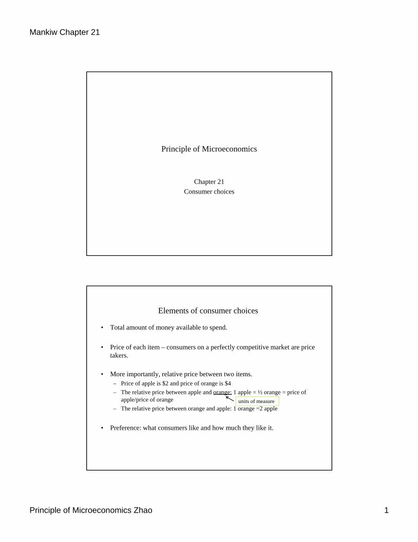
Elements of consumer choices

• Total amount of money available to spend.

• Price of each item – consumers on a perfectly competitive market are price takers.

• More importantly, relative price between two items.– Price of apple is $2 and price of orange is $4

– The relative price between apple and orange: 1 apple = ½ orange = price of apple/price of orange

– The relative price between orange and apple: 1 orange =2 apple

• Preference: what consumers like and how much they like it.

units of measure


Mankiw Chapter 21

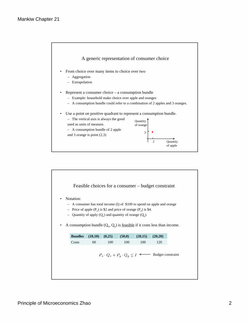
A generic representation of consumer choice

• From choice over many items to choice over two– Aggregation

– Extrapolation

• Represent a consumer choice – a consumption bundle– Example: household make choice over apple and oranges

– A consumption bundle could refer to a combination of 2 apples and 3 oranges.

• Use a point on positive quadrant to represent a consumption bundle. – The vertical axis is always the good

used as units of measure.

– A consumption bundle of 2 apple

and 3 orange is point (2,3)

Quantity of apple

Quantity of orange

2

3

Feasible choices for a consumer – budget constraint

• Notation:– A consumer has total income (I) of $100 to spend on apple and orange

– Price of apple (Px) is $2 and price of orange (Py) is $4.

– Quantity of apply (Qx) and quantity of orange (Qy)

• A consumption bundle (Qx, Qy) is feasible if it costs less than income.

Bundles (10,10) (0,25) (50,0) (20,15) (20,20)

Costs 60 100 100 100 120

Budget constraint


Mankiw Chapter 21

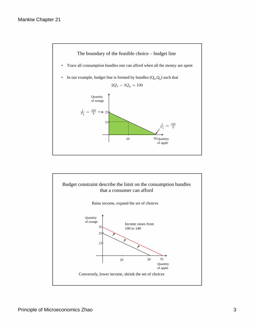
The boundary of the feasible choice – budget line

• Trace all consumption bundles one can afford when all the money are spent

• In our example, budget line is formed by bundles (Qx,Qy) such that

Quantity of apple

Quantity of orange

50

25

20

15

Budget constraint describe the limit on the consumption bundles that a consumer can afford

Raise income, expand the set of choices

Quantity of apple

Quantity of orange

50

25

20

15

Conversely, lower income, shrink the set of choices

35

70

Income raises from 100 to 140


Mankiw Chapter 21

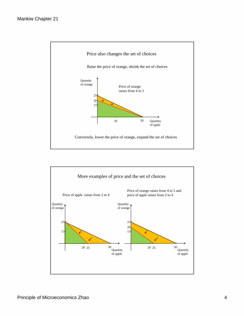
Price also changes the set of choices

Raise the price of orange, shrink the set of choices

Quantity of apple

Quantity of orange

50

25

20

15

Conversely, lower the price of orange, expand the set of choices

20

Price of orange raises from 4 to 5

More examples of price and the set of choices

Quantity of apple

Quantity of orange

50

25

20

15

Price of apple raises from 2 to 4

25Quantity of apple

Quantity of orange

50

25

20

1520

Price of orange raises from 4 to 5 and price of apple raises from 2 to 4

25


Mankiw Chapter 21

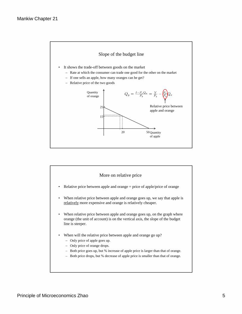
Slope of the budget line

• It shows the trade-off between goods on the market– Rate at which the consumer can trade one good for the other on the market

– If one sells an apple, how many oranges can he get?

– Relative price of the two goods

Quantity of apple

Quantity of orange

50

25

20

15

Relative price between apple and orange

More on relative price

• Relative price between apple and orange = price of apple/price of orange

• When relative price between apple and orange goes up, we say that apple is relatively more expensive and orange is relatively cheaper.

• When relative price between apple and orange goes up, on the graph where orange (the unit of account) is on the vertical axis, the slope of the budget line is steeper.

• When will the relative price between apple and orange go up?– Only price of apple goes up.

– Only price of orange drops.

– Both price goes up, but % increase of apple price is larger than that of orange.

– Both price drops, but % decrease of apple price is smaller than that of orange.


Mankiw Chapter 21

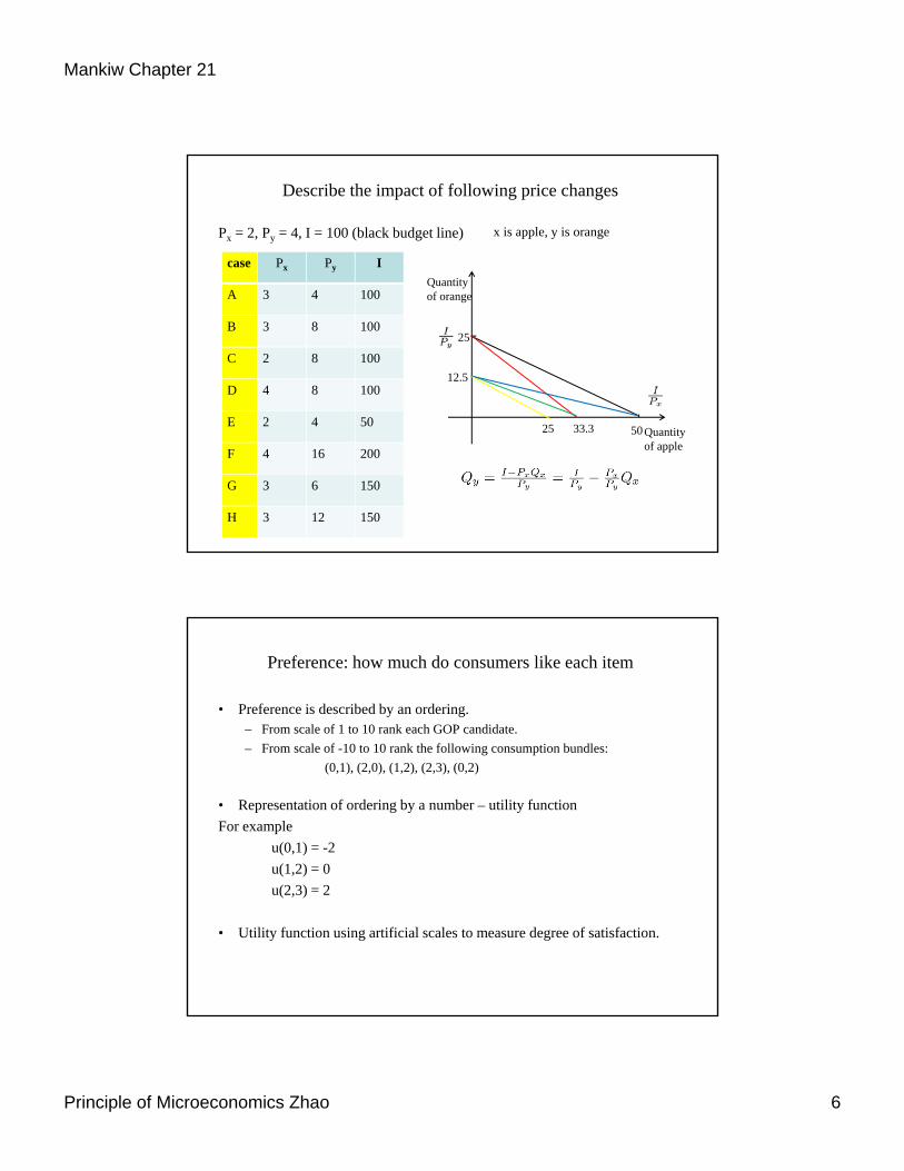
Describe the impact of following price changes

Px = 2, Py = 4, I = 100 (black budget line)

Quantity of apple

Quantity of orange

50

25

12.5

25 33.3

case Px Py I

A 3 4 100

B 3 8 100

C 2 8 100

D 4 8 100

E 2 4 50

F 4 16 200

G 3 6 150

H 3 12 150

x is apple, y is orange

Preference: how much do consumers like each item

• Preference is described by an ordering.– From scale of 1 to 10 rank each GOP candidate.

– From scale of -10 to 10 rank the following consumption bundles:

(0,1), (2,0), (1,2), (2,3), (0,2)

• Representation of ordering by a number – utility function

For example

u(0,1) = -2

u(1,2) = 0

u(2,3) = 2

• Utility function using artificial scales to measure degree of satisfaction.


Mankiw Chapter 21

Basic logical requirements for preference ordering

• Completeness: When compare two bundles, red and blue

A) Red is preferred to blue

B) Blue is preferred to red

C) Indifferent between red and blue

D) Don’t know

• Transitivity: If you say that red is better than blue, blue is better than green, then you can’t say that green is better than red.

• No lexicographical ordering.

More apple is always better, no matter how much orange I get. If two bundles have the same amount of apples, then I prefer the one with more oranges.

Application of contour maps --Topographic maps

• Contour map: 2-D representation of 3-D object


Mankiw Chapter 21

Topographic maps of Stone mountain

US surface temperature contour maps


Mankiw Chapter 21

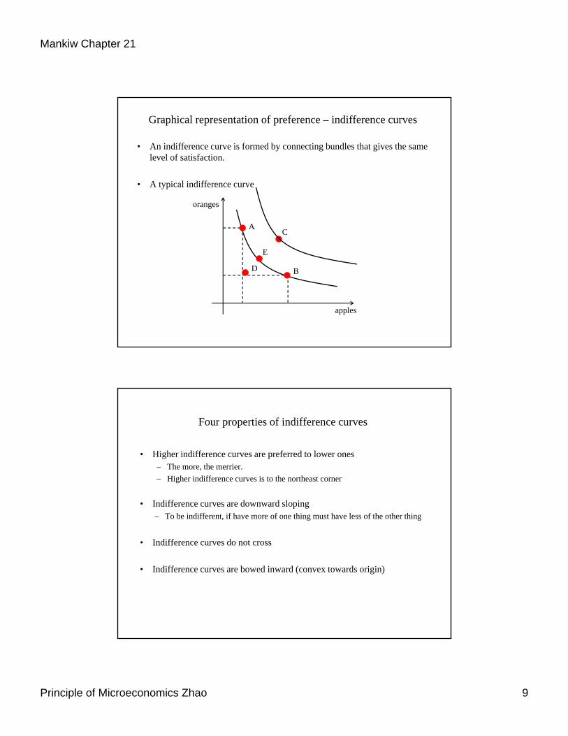
Graphical representation of preference – indifference curves

• An indifference curve is formed by connecting bundles that gives the same level of satisfaction.

• A typical indifference curve

apples

oranges

A

B

C

D

E

Four properties of indifference curves

• Higher indifference curves are preferred to lower ones– The more, the merrier.

– Higher indifference curves is to the northeast corner

• Indifference curves are downward sloping– To be indifferent, if have more of one thing must have less of the other thing

• Indifference curves do not cross

• Indifference curves are bowed inward (convex towards origin)


Mankiw Chapter 21

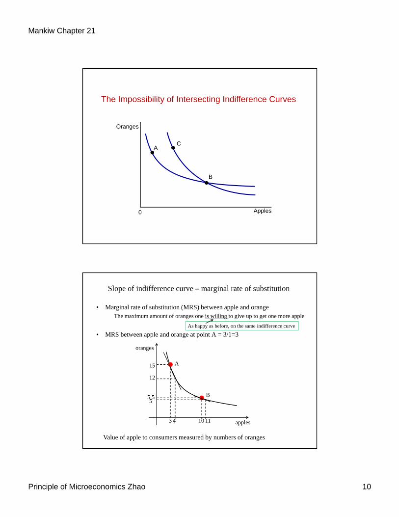
The Impossibility of Intersecting Indifference Curves

Oranges

Apples0

C

B

A

Slope of indifference curve – marginal rate of substitution

• Marginal rate of substitution (MRS) between apple and orangeThe maximum amount of oranges one is willing to give up to get one more apple

• MRS between apple and orange at point A = 3/1=3

apples

oranges

A

B

3 4

15

12

10 11

55.5

As happy as before, on the same indifference curve

Value of apple to consumers measured by numbers of oranges


Mankiw Chapter 21

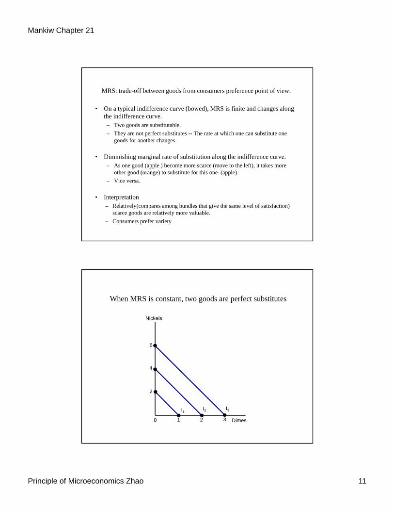
MRS: trade-off between goods from consumers preference point of view.

• On a typical indifference curve (bowed), MRS is finite and changes along the indifference curve.

– Two goods are substitutable.

– They are not perfect substitutes -- The rate at which one can substitute one goods for another changes.

• Diminishing marginal rate of substitution along the indifference curve.– As one good (apple ) become more scarce (move to the left), it takes more

other good (orange) to substitute for this one. (apple).

– Vice versa.

• Interpretation– Relatively(compares among bundles that give the same level of satisfaction)

scarce goods are relatively more valuable.

– Consumers prefer variety

When MRS is constant, two goods are perfect substitutes

Nickels

6

2

4

Dimes 0 1 32

I1 I2 I3


Mankiw Chapter 21

When MRS is either infinite or zero, two goods are perfect complements

Leftshoes

Rightshoes

0 54

5

I2

I1

6

Constrained optimization

I want to live at the warmest place in the state of Georgia.


Mankiw Chapter 21

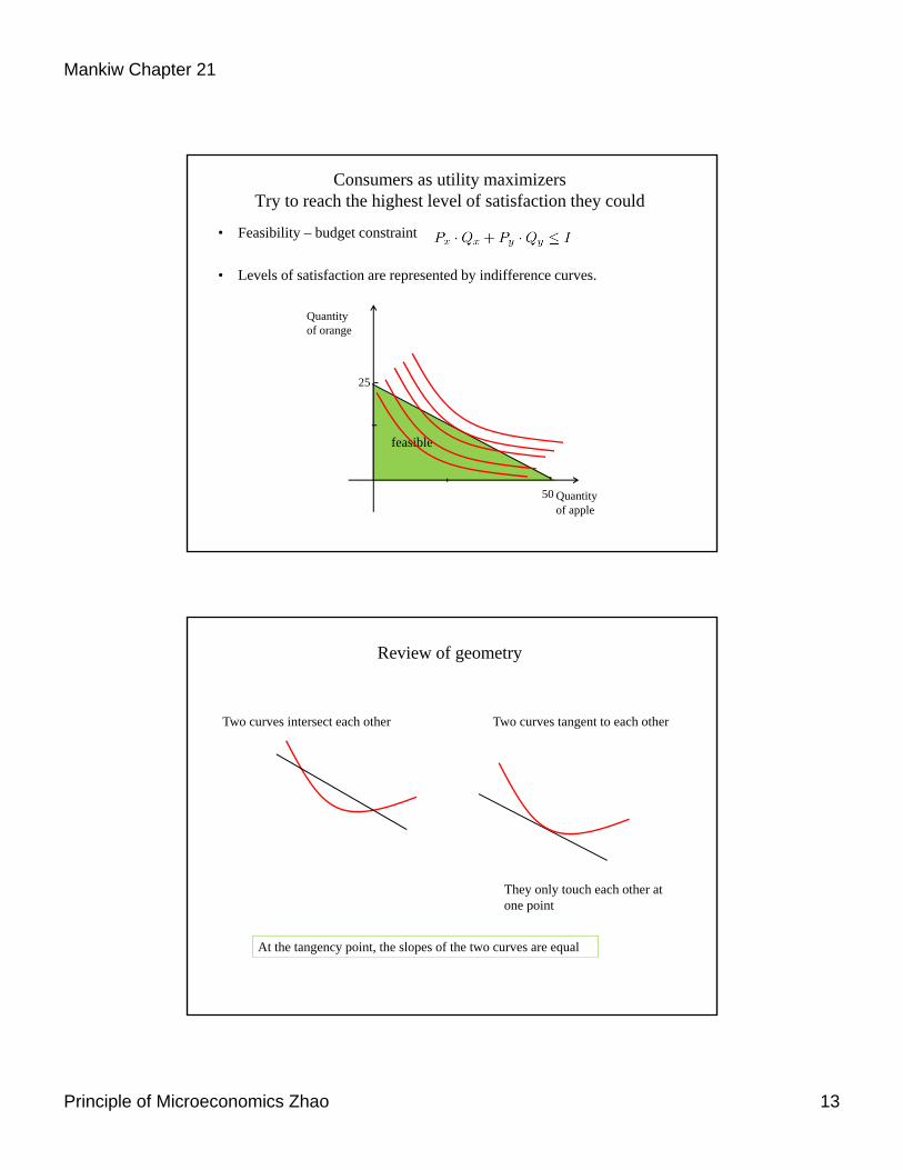
Consumers as utility maximizersTry to reach the highest level of satisfaction they could

• Feasibility – budget constraint

• Levels of satisfaction are represented by indifference curves.

Quantity of apple

Quantity of orange

50

25

feasible

Review of geometry

Two curves intersect each other Two curves tangent to each other

They only touch each other at one point

At the tangency point, the slopes of the two curves are equal


Mankiw Chapter 21

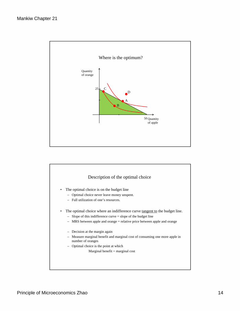
Where is the optimum?

Quantity of apple

Quantity of orange

50

25D

A

B

C

Description of the optimal choice

• The optimal choice is on the budget line– Optimal choice never leave money unspent.

– Full utilization of one’s resources.

• The optimal choice where an indifference curve tangent to the budget line.– Slope of this indifference curve = slope of the budget line

– MRS between apple and orange = relative price between apple and orange

– Decision at the margin again

– Measure marginal benefit and marginal cost of consuming one more apple in number of oranges

– Optimal choice is the point at which

Marginal benefit = marginal cost


Mankiw Chapter 21

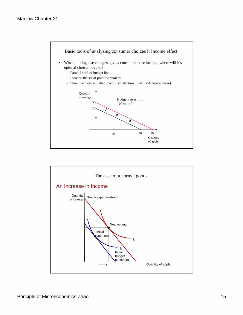
Basic tools of analyzing consumer choices I: Income effect

• When nothing else changes, give a consumer more income, where will his optimal choice move to?

– Parallel shift of budget line

– Increase the set of possible choices

– Should achieve a higher level of satisfaction. (new indifference curve)

Quantity of apple

Quantity of orange

50

25

20

15

35

70

Budget raises from 100 to 140

An Increase in Income

Quantityof orange

Quantity of apple0

New budget constraint

I2

I1

New optimum

Initialbudgetconstraint

Initial optimum

The case of a normal goods


Mankiw Chapter 21

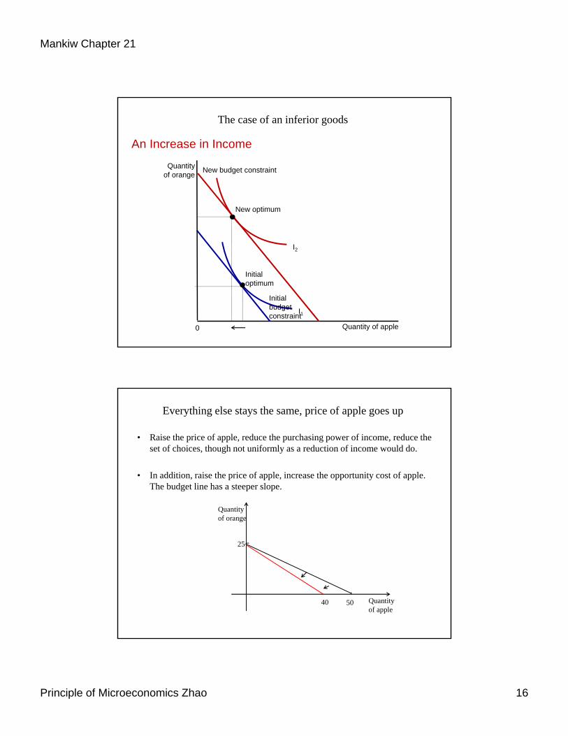
An Increase in Income

Quantityof orange

Quantity of apple0

New budget constraint

I2

I1

New optimum

Initialbudgetconstraint

Initial optimum

The case of an inferior goods

Everything else stays the same, price of apple goes up

• Raise the price of apple, reduce the purchasing power of income, reduce the set of choices, though not uniformly as a reduction of income would do.

• In addition, raise the price of apple, increase the opportunity cost of apple. The budget line has a steeper slope.

Quantity of apple

Quantity of orange

50

25

40


Mankiw Chapter 21

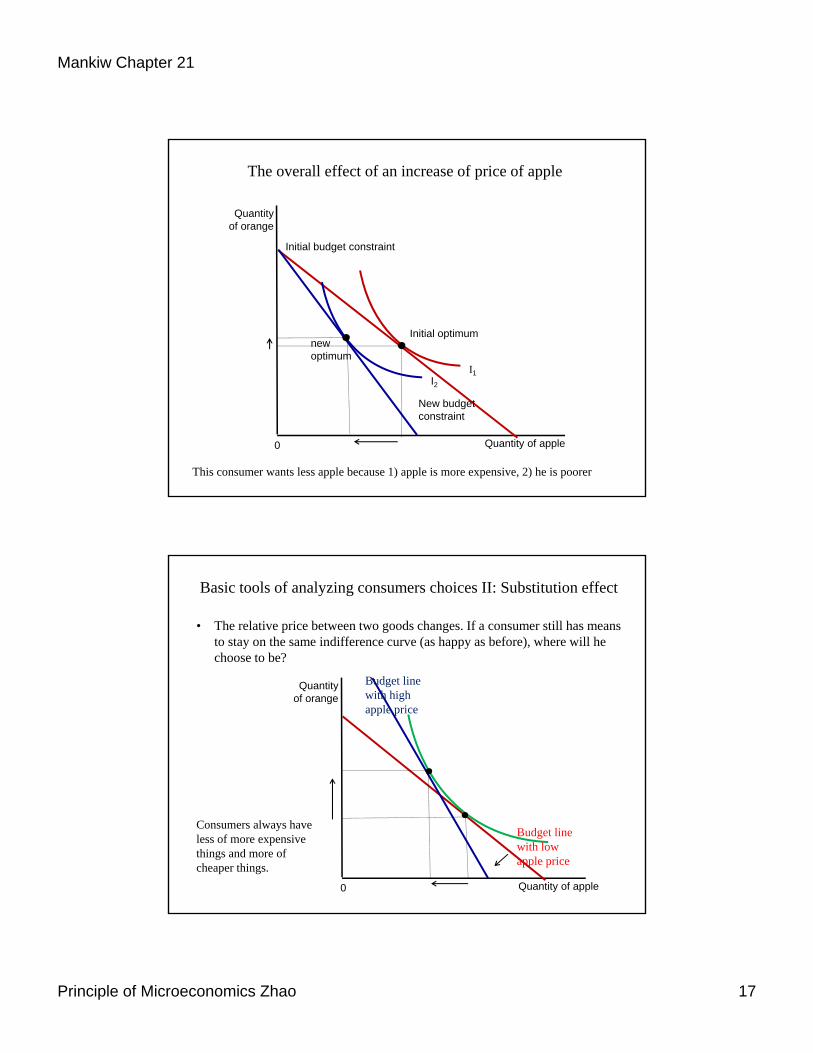
The overall effect of an increase of price of apple

Quantityof orange

Quantity of apple0

Initial budget constraint

I1I2

Initial optimum

New budgetconstraint

new optimum

This consumer wants less apple because 1) apple is more expensive, 2) he is poorer

• The relative price between two goods changes. If a consumer still has means to stay on the same indifference curve (as happy as before), where will he choose to be?

Basic tools of analyzing consumers choices II: Substitution effect

Quantityof orange

Quantity of apple0

Budget line with high apple price

Budget line with low apple price

Consumers always have less of more expensive things and more of cheaper things.


Mankiw Chapter 21

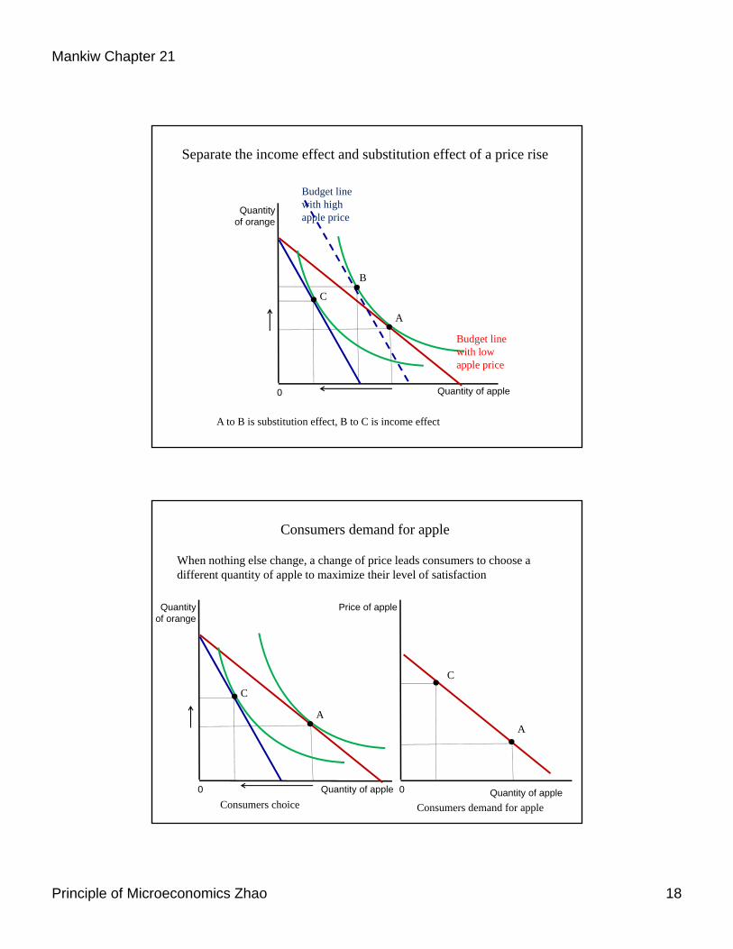
Separate the income effect and substitution effect of a price rise

Quantityof orange

Quantity of apple0

Budget line with high apple price

Budget line with low apple price

A

B

C

A to B is substitution effect, B to C is income effect

Consumers demand for apple

When nothing else change, a change of price leads consumers to choose a different quantity of apple to maximize their level of satisfaction

Quantityof orange

Quantity of apple0

A

C

Price of apple

Quantity of apple0

A

C

Consumers choice Consumers demand for apple


Mankiw Chapter 21

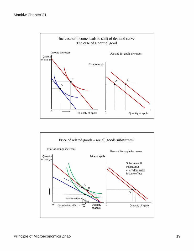
Increase of income leads to shift of demand curveThe case of a normal good

Quantityof orange

Quantity of apple0

B

A

Price of apple

Quantity of apple0

A B

Income increases Demand for apple increases

Price of related goods – are all goods substitutes?

Quantityof orange

Quantity of apple

0

A

B

Price of apple

Quantity of apple0

AB

Price of orange increasesDemand for apple increases

C

Income effect

Substitution effect

Substitutes, if substitution effect dominatesincome effect


Mankiw Chapter 21

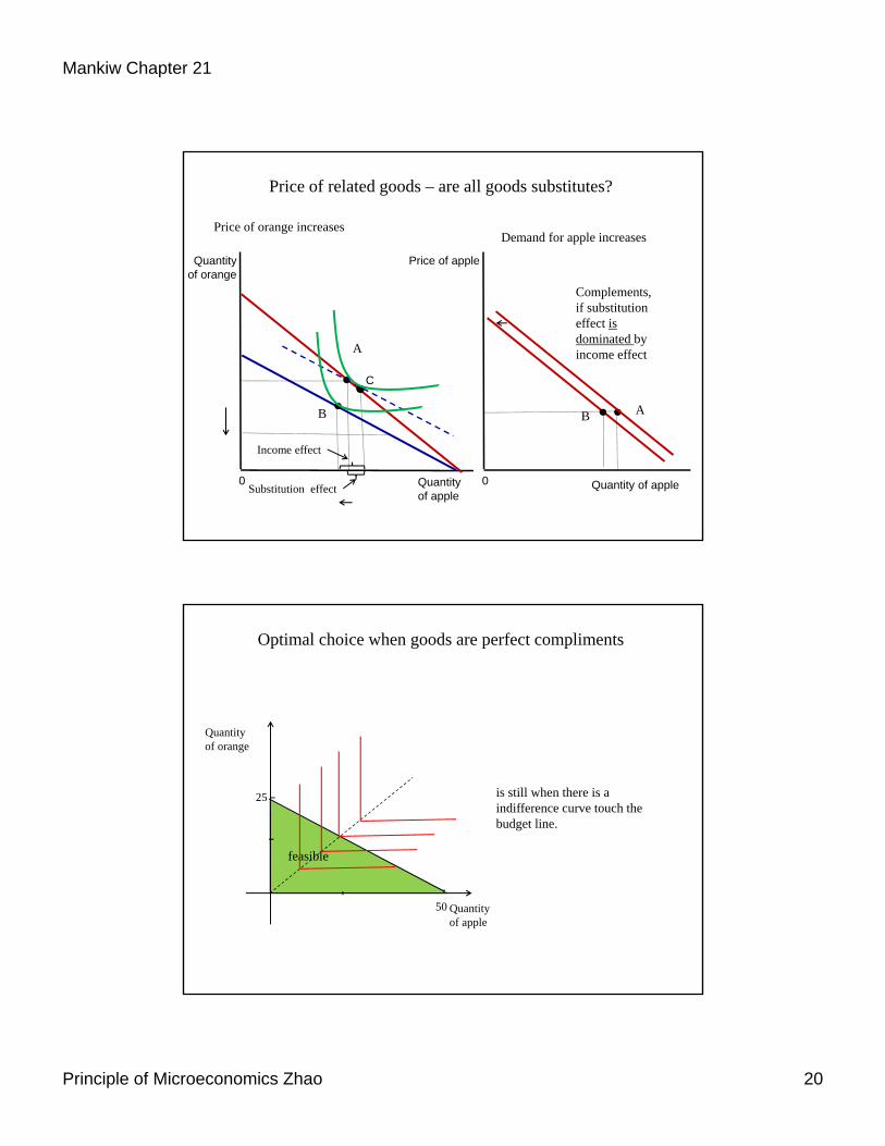
Price of related goods – are all goods substitutes?

Quantityof orange

Quantity of apple

0

A

B

Price of apple

Quantity of apple0

AB

Price of orange increasesDemand for apple increases

C

Income effect

Substitution effect

Complements, if substitution effect is dominated by income effect

Optimal choice when goods are perfect compliments

Quantity of apple

Quantity of orange

50

25

feasible

is still when there is a indifference curve touch the budget line.


Mankiw Chapter 21

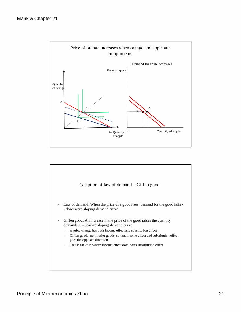
Price of orange increases when orange and apple are compliments

Quantity of apple

Quantity of orange

50

25

A

B

Price of apple

Quantity of apple0

AB

Demand for apple decreases

Exception of law of demand – Giffen good

• Law of demand: When the price of a good rises, demand for the good falls -- downward sloping demand curve

• Giffen good: An increase in the price of the good raises the quantity demanded. – upward sloping demand curve

– A price change has both income effect and substitution effect

– Giffen goods are inferior goods, so that income effect and substitution effect goes the opposite direction.

– This is the case where income effect dominates substitution effect


Mankiw Chapter 21

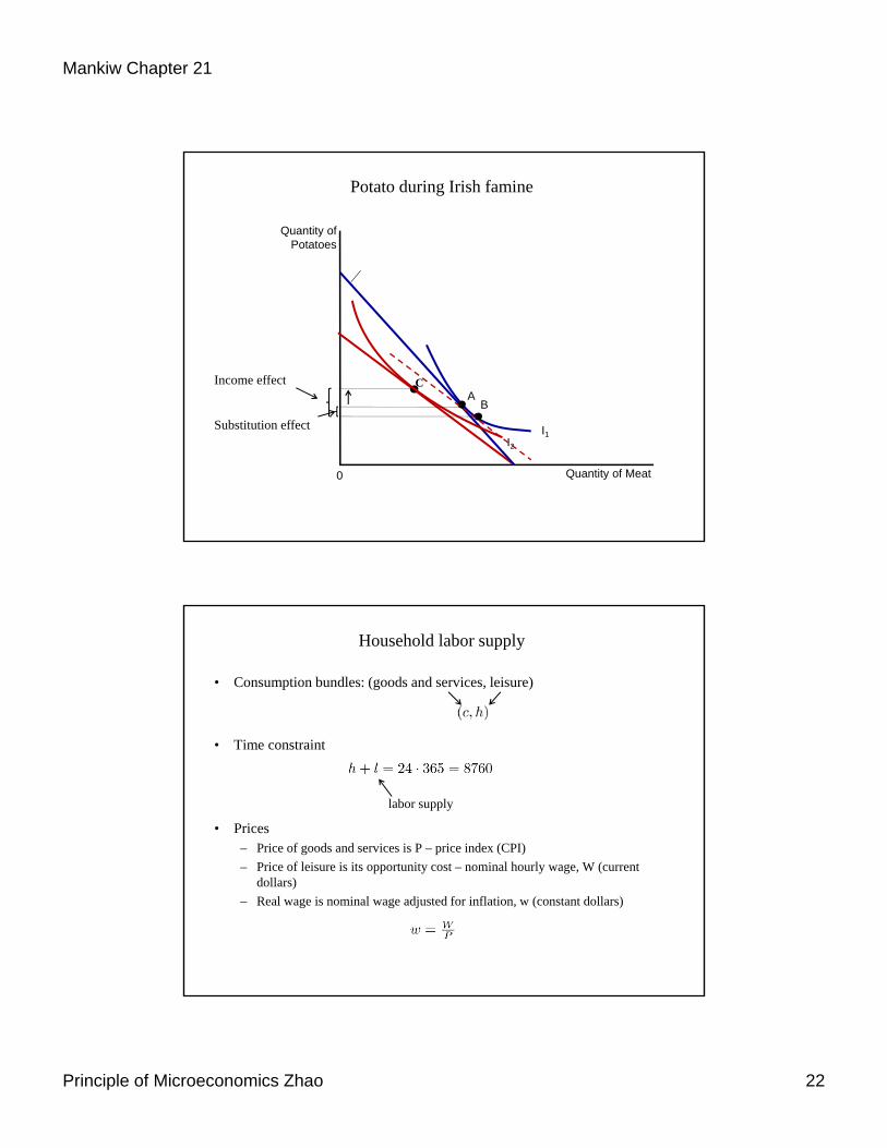
Potato during Irish famine

Quantity ofPotatoes

Quantity of Meat0

I1

AB

C

I2

Substitution effect

Income effect

Household labor supply

• Consumption bundles: (goods and services, leisure)

• Time constraint

• Prices– Price of goods and services is P – price index (CPI)

– Price of leisure is its opportunity cost – nominal hourly wage, W (current dollars)

– Real wage is nominal wage adjusted for inflation, w (constant dollars)

labor supply


Mankiw Chapter 21

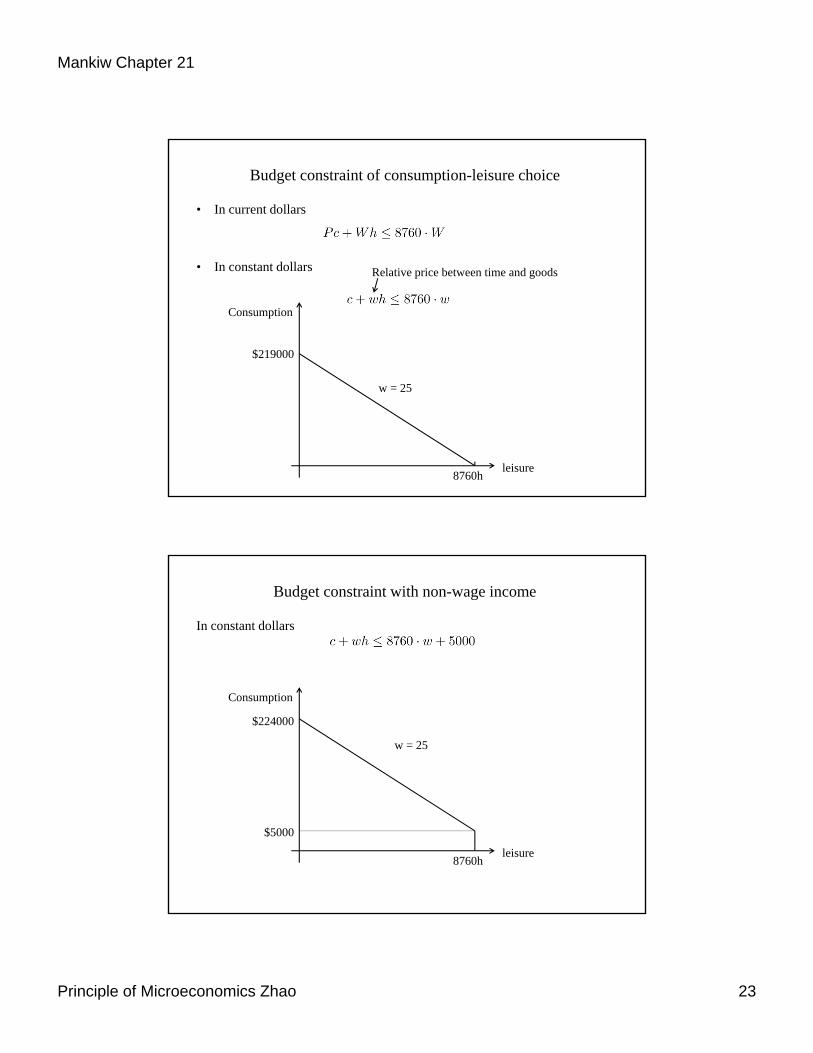
Budget constraint of consumption-leisure choice

• In current dollars

• In constant dollars Relative price between time and goods

Consumption

leisure8760h

w = 25

$219000

Budget constraint with non-wage income

In constant dollars

Consumption

leisure8760h

w = 25

$224000

$5000


Mankiw Chapter 21

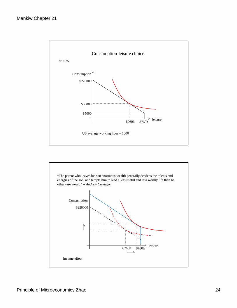
Consumption-leisure choice

Consumption

leisure8760h

w = 25

$220000

$5000

$50000

6960h

US average working hour = 1800

“The parent who leaves his son enormous wealth generally deadens the talents and energies of the son, and tempts him to lead a less useful and less worthy life than he otherwise would” -- Andrew Carnegie

Consumption

leisure8760h

$220000

6760h

Income effect


Mankiw Chapter 21

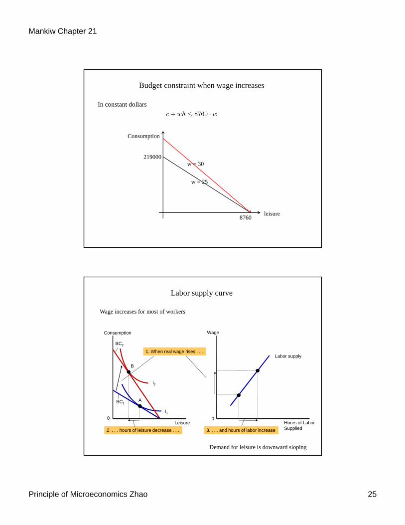
Budget constraint when wage increases

In constant dollars

Consumption

leisure8760

w = 25

219000w = 30

Labor supply curve

Wage increases for most of workers

Consumption

Leisure0

Wage

Hours of LaborSupplied

0

Labor supply

I2

I1

BC2

BC1A

B

1. When real wage rises . . .

2. . . . hours of leisure decrease . . . 3. . . . and hours of labor increase

Demand for leisure is downward sloping


Mankiw Chapter 21

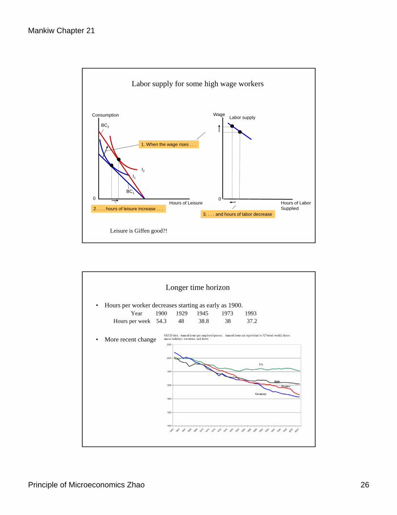
Labor supply for some high wage workers

Consumption

Hours of Leisure0

Wage

Hours of LaborSupplied

0

Labor supply

I2I1

BC2

BC1

1. When the wage rises . . .

2. . . . hours of leisure increase . . .3. . . . and hours of labor decrease

Leisure is Giffen good?!

Longer time horizon

• Hours per worker decreases starting as early as 1900.Year 1900 1929 1945 1973 1993

Hours per week 54.3 48 38.8 38 37.2

• More recent change


Mankiw Chapter 21

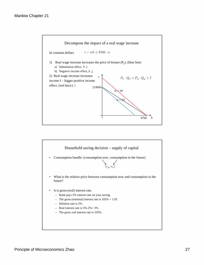
Decompose the impact of a real wage increase

In constant dollars

1) Real wage increase increases the price of leisure (Py). (blue line)a) Substitution effect,

b) Negative income effect,

2) Real wage increase increases

income I – bigger positive income

effect. (red line)

c

8760

w = 25

219000w = 30

h

Household saving decision – supply of capital

• Consumption bundle: (consumption now, consumption in the future)

• What is the relative price between consumption now and consumption in the future?

• It is gross (real) interest rate. – Bank pays 5% interest rate on your saving.

– The gross (nominal) interest rate is 105% = 1.05

– Inflation rate is 2%.

– Real interest rate is 5%-2%= 3%

– The gross real interest rate is 103%.


Mankiw Chapter 21

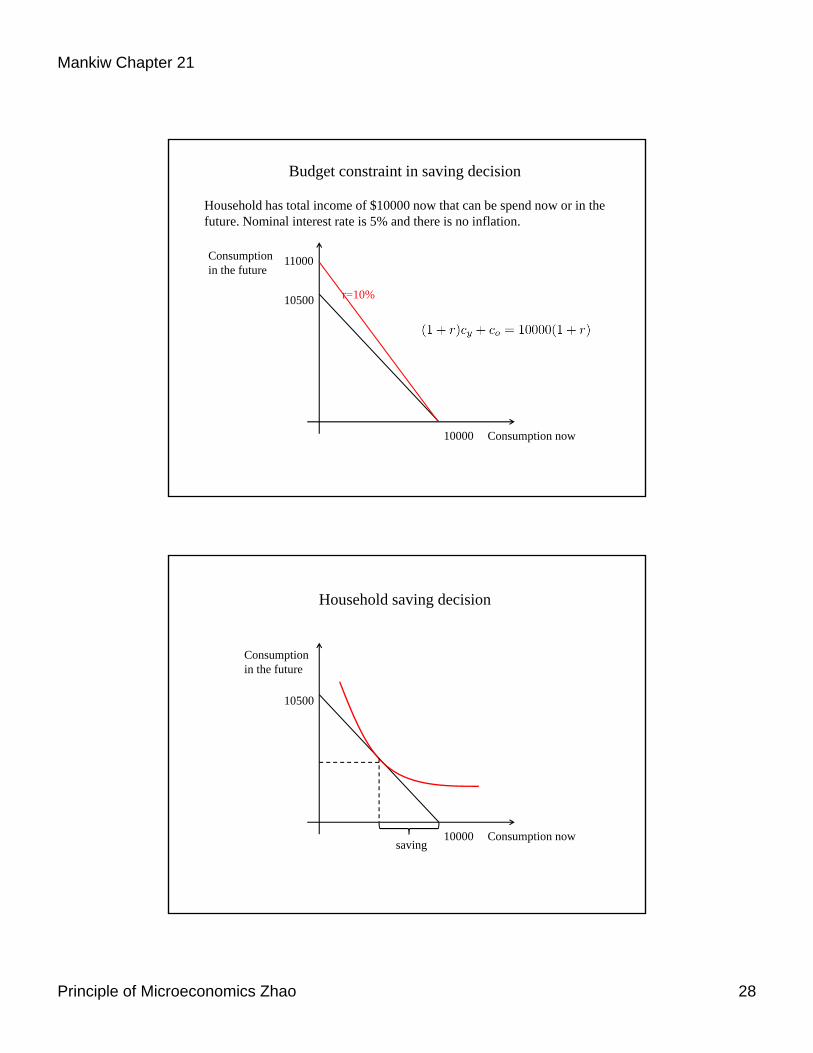
Budget constraint in saving decision

Household has total income of $10000 now that can be spend now or in the future. Nominal interest rate is 5% and there is no inflation.

Consumption now

Consumption in the future

10000

10500

11000

r=10%

Household saving decision

Consumption in the future

10000

10500

Consumption nowsaving


Mankiw Chapter 21

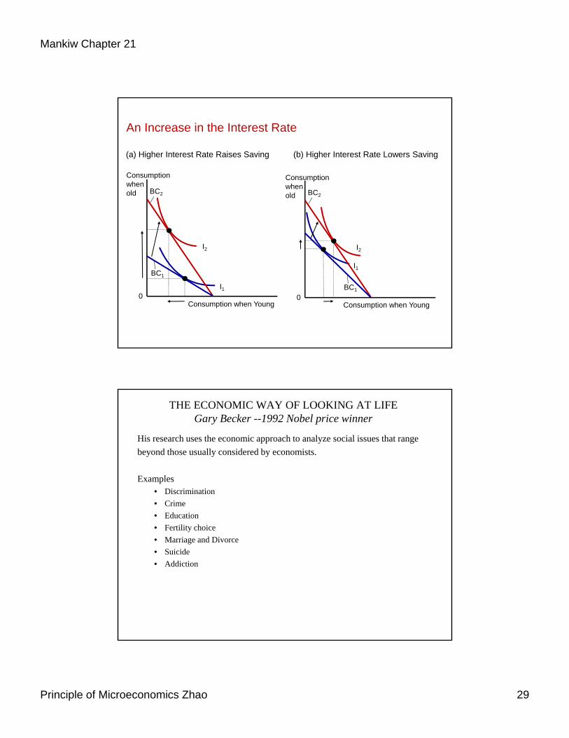
An Increase in the Interest Rate

Consumptionwhenold

(a) Higher Interest Rate Raises Saving

Consumption when Young0

I2

I1

BC2

BC1

Consumptionwhenold

(b) Higher Interest Rate Lowers Saving

Consumption when Young0

I2

I1

BC2

BC1

THE ECONOMIC WAY OF LOOKING AT LIFEGary Becker --1992 Nobel price winner

His research uses the economic approach to analyze social issues that range

beyond those usually considered by economists.

Examples• Discrimination

• Crime

• Education

• Fertility choice

• Marriage and Divorce

• Suicide

• Addiction


Mankiw Chapter 21

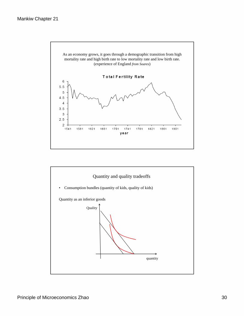
As an economy grows, it goes through a demographic transition from high mortality rate and high birth rate to low mortality rate and low birth rate.

(experience of England from Soares)

Quantity and quality tradeoffs

• Consumption bundles (quantity of kids, quality of kids)

Quantity as an inferior goods

Quality

quantity


Mankiw Chapter 21

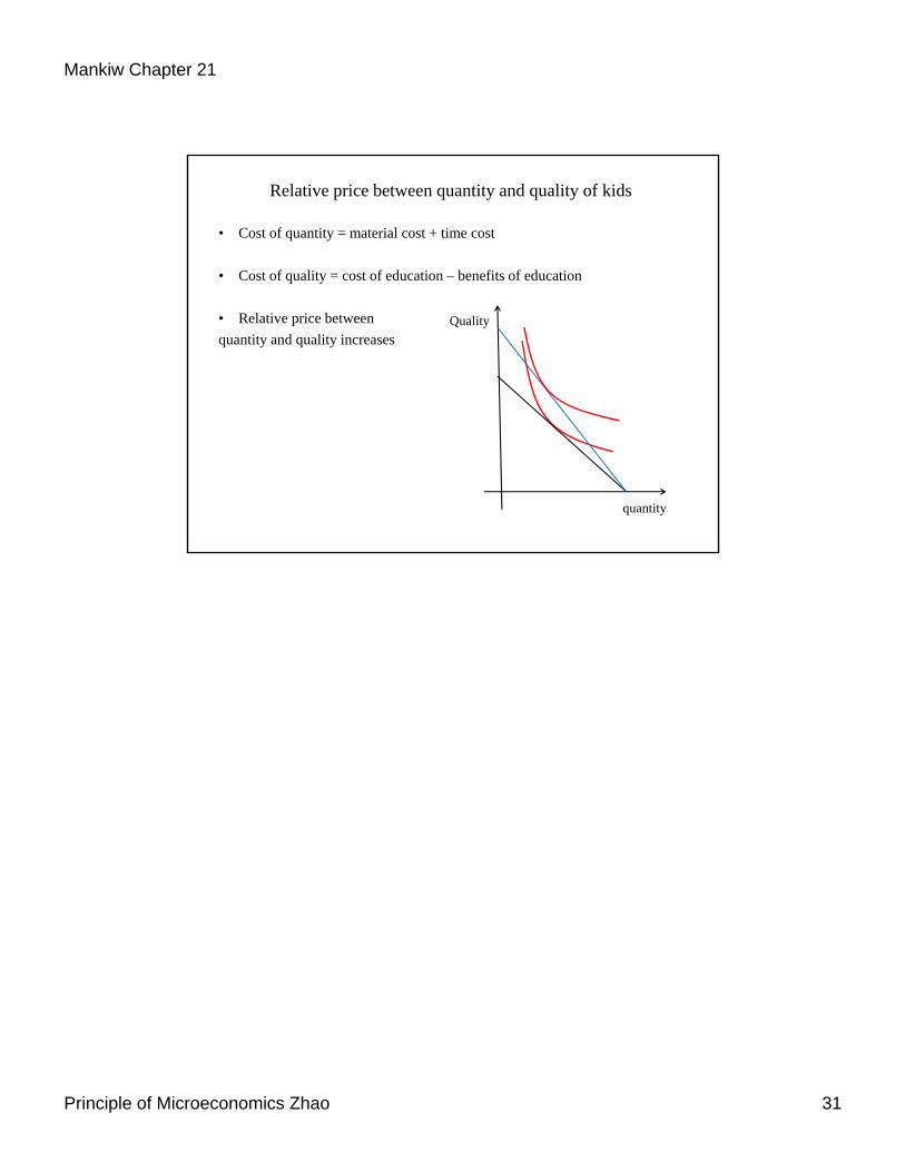
Relative price between quantity and quality of kids

• Cost of quantity = material cost + time cost

• Cost of quality = cost of education – benefits of education

• Relative price between

quantity and quality increasesQuality

quantity

Documents

Mankiw Chapter 21 - Amazon S3s3.amazonaws.com/zanran_storage/user... · Principle of Microeconomics Zhao 2 Mankiw Chapter 21 A generic representation of consumer choice • From choice