Embed Size (px)
Citation preview

Manipulations in Spin and Space: Tensors, Rotations, and
Average Hamiltonian Theory
Len Mueller
University of California,Riverside

Hamiltonians in NMR
• I, B in lab frame• A is a second-rank Cartesian tensor and is a molecular-level property that depends
on local geometry, electronic structure, and orientation within the lab frame• Can manipulate the Hamiltonian through both the spin and space components• Need a working knowledge of both tensors and rotations and techniques for
solving time-dependent quantum mechanical problems
λλλλ SIcH ⋅⋅= A
...,,...,
JD,σ,A =
=λ
λ IBS
=
zzyzxz
zyyyxy
zxyxxx
aaaaaaaaa
A

Part I: Tensors and Rotations in NMR
Len Mueller
University of California,Riverside

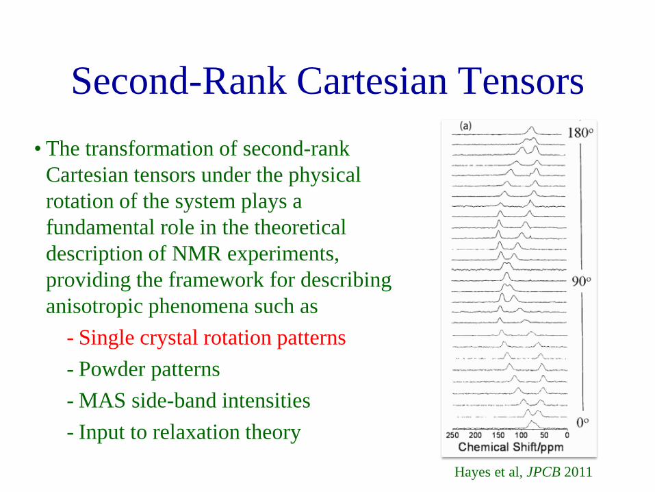
Second-Rank Cartesian Tensors • The transformation of second-rank
Cartesian tensors under the physical rotation of the system plays a fundamental role in the theoretical description of NMR experiments, providing the framework for describing anisotropic phenomena such as
- Single crystal rotation patterns- Powder patterns- MAS side-band intensities- Input to relaxation theory
A A′R
Second-Rank Cartesian Tensors • The transformation of second-rank
Cartesian tensors under the physical rotation of the system plays a fundamental role in the theoretical description of NMR experiments, providing the framework for describing anisotropic phenomena such as
- Single crystal rotation patterns- Powder patterns- MAS side-band intensities- Input to relaxation theory
Hayes et al, JPCB 2011

Second-Rank Cartesian Tensors • The transformation of second-rank
Cartesian tensors under the physical rotation of the system plays a fundamental role in the theoretical description of NMR experiments, providing the framework for describing anisotropic phenomena such as
- Single crystal rotation patterns- Powder patterns- MAS side-band intensities- Input to relaxation theory 13C Chemical Shift (ppm)

Second-Rank Cartesian Tensors • The transformation of second-rank
Cartesian tensors under the physical rotation of the system plays a fundamental role in the theoretical description of NMR experiments, providing the framework for describing anisotropic phenomena such as
- Single crystal rotation patterns- Powder patterns- MAS side-band intensities- Input to relaxation theory 29Si Chemical Shift (ppm)

Second-Rank Cartesian Tensors • The transformation of second-rank
Cartesian tensors under the physical rotation of the system plays a fundamental role in the theoretical description of NMR experiments, providing the framework for describing anisotropic phenomena such as
- Single crystal rotation patterns- Powder patterns- MAS side-band intensities- Input to relaxation theory

Tensors and Rotations• Two ways to treat this are the direct rotation in Cartesian form
and the decomposition of the Cartesian tensor into irreducible spherical components that rotate in subgroups of rank 0, 1, and 2 – you need to know how to manipulate tensors in both forms
– these must give the same results!
( ) pkRkqp
k
kpqk D AA Ω=′ ∑
−=
)(
A A′R
1−=′ RARA

Tensors and Rotations:The Problem
• As written and applied in most standard NMR texts they do not!• There is a curious need to switch sense of rotation for Cartesian
and spherical tensors to effect the same transformation
( ) pkRkqp
k
kpqk D AA Ω=′ ∑
−=
)(
A A′R
1−=′ RARA

Tensors and Rotations:The Problem
A A′R
1−=′ RARA
• A problem that is rarely noted and has not been reconciled• Not convention, but fundamental
( ) pkRkqp
k
kpqk D AA 1
)(−Ω=′ ∑
−=
• As written and applied in most standard NMR texts they do not!• There is a curious need to switch sense of rotation for Cartesian
and spherical tensors to effect the same transformation

Goals of this Part 1• Review the transformation of second-rank tensors under rotation
in both Cartesian and spherical tensor form• Reconcile the inconsistency in the sense of rotation necessary to
produce equivalent transformations• A uniform approach to the rotation of a physical system and the
corresponding transformation of the spatial components of the NMR Hamiltonian – expressed as either Cartesian or spherical tensors
Mueller, Concepts in Magnetic Resonance A, 38A, 221-235 (2011)

Outline for Part 1• Construction of the NMR Hamiltonian in terms of second-rank tensors
• Cartesian rotation matrices• Irreducible spherical tensor basis• A consistent treatment of rotations in spherical tensor form
• Example: Rotation of an ab intio chemical shielding tensor
• What went wrong and a few words of caution

Hamiltonians in NMR
• I, B in lab frame• A is a second-rank Cartesian tensor and is a molecular-level
property that depends on local geometry, electronic structure, and orientation within the lab frame
λλλλ SIcH ⋅⋅= A
...,,...,
JD,σ,A =
=λ
λ IBS
=
zzyzxz
zyyyxy
zxyxxx
aaaaaaaaa
A
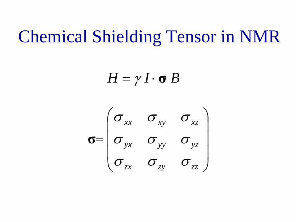
Chemical Shielding Tensor in NMR
BIH ⋅⋅= σγ
=
zzzyzx
yzyyyx
xzxyxx
σσσσσσσσσ
σ
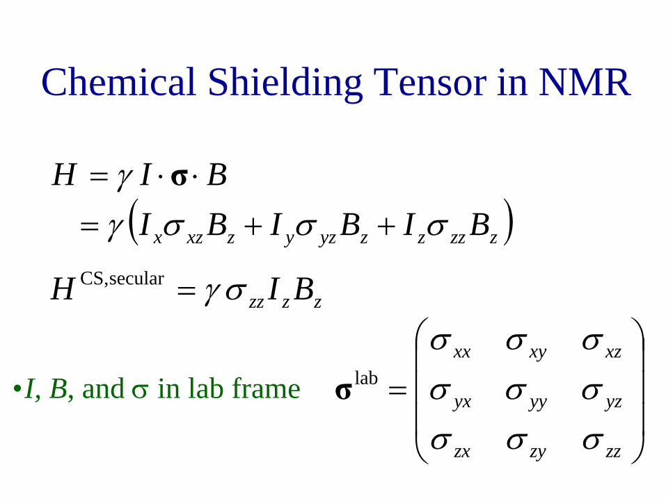
Chemical Shielding Tensor in NMR
( )zzzzzyzyzxzx BIBIBIBIH
σσσγγ
++=⋅⋅= σ
=
zzzyzx
yzyyyx
xzxyxx
σσσσσσσσσ
labσ•I, B, and σ in lab frame
zzzz BIH σγ=secularCS,

Principal Axis System
=
ZZ
YY
XX
σσ
σ
000000
PASσ
Often represent tensors as ellipsoids with PAS components as axes. This is not a completely accurate mapping (but still useful).

Orientation Dependence
1
000000
−
=
RR
ZZ
YY
XX
zzzyzx
yzyyyx
xzxyxx
σσ
σ
σσσσσσσσσ
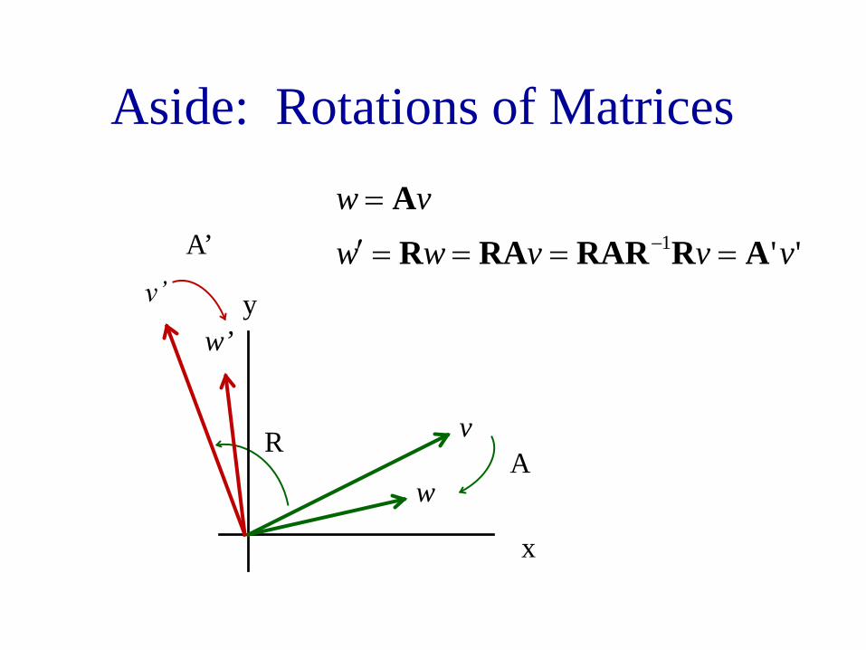
Aside: Rotations of Matrices
''1 vvvwwvw
ARRARRARA
====′
=−
y
x
v
wA
w’
A’
R

Rotations and Euler Angles
ZYZ Convention

Rotation Matrices and Euler Angles
( )
−+−+−−−
=βγβγβ
βαγαγβαγαγβαβαγαγβαγαγβα
γβαcossinsincossin
sinsincoscossincossinsincoscoscossinsincoscossinsincoscossinsincoscoscos
,,A
Active Rotation: Rotate body-fixed frame relative to the observer-fixed frame
Bouten, Physica 42 (1969) 572-580

Rotation Matrices and Euler Angles
( )
+−−−
−+−=
ββαβαγβγαγβαγαγβαγβγαγβαγαγβα
γβαcossinsinsincos
sinsincoscossincossincossinsincoscoscossinsincoscoscossinsinsincoscoscos
,,P
Passive Rotation: Rotate observer-fixed frame relative to the body-fixed frame
Bouten, Physica 42 (1969) 572-580

Constructing the Rotation Matrix
Active
x
y
x
y
x
y
Passive
( )
−=
1000cossin0sincos
αααα
αza ( )
−=
1000cossin0sincos
αααα
αzp

Constructing the Rotation MatrixActive Passive
( )
−=
1000cossin0sincos
αααα
αza ( )
−=
1000cossin0sincos
αααα
αzp
( )
−=
ββ
βββ
cos0sin010
sin0cos
ya ( )
−=
ββ
βββ
cos0sin010
sin0cos
yp
( ) ( ) ( ) ( )αβγγβα ZYZ pppP =,,( ) ( ) ( ) ( )αβγγβα ZYZ aaaA =,,
Easy! Rotatable frame is the observer frame so just multiply
Hard! Rotatable axes X,Y,Z are not unit axes in observer frame x,y,z. But they can easily be transformed into rotations in the observer (space-fixed) frame; note the reversal in the order of angles (problem set !)
( ) ( ) ( ) ( )γβαγβα zyz aaaA =,,

Active vs. Passive Rotation
x
y
x
y
x
y
( ) ( )γβαγβα ,,,, 1−= AP
Active Passive

Active vs. Passive:Is there a Difference?
x
y
x
y
=
z
y
x
z
y
x
bbb
aaa
R

Active vs. Passive: Is there a Difference?
x
y
x
y
=
z
y
x
z
y
x
bbb
aaa
R

Bases and Coordinates:A Critical Distinction
• Bases
iRyxxx xiyxi
Rz ˆˆsinˆcossincos
01
cossinsincos
ˆˆ,
∑=
=+=
=
−== αα
αα
αααα
R
ixiyxi
iixyxi
x
yx
yx
y
x
y
x
y
x
cRcRc
cccc
cc
cc
cc
1
,,
cossinsincos
cossinsincos
−
==∑∑ ==′
+−
=
−=
=
′′
αααα
αααα
R
• Asymmetry between bases and coefficients (coordinates) transform in the opposite sense
• Well-known correspondence in linear algebra
• Coordinates:

Tensors and Rotations
Cartesian
( ) pkRkqp
k
kpqk D AA Ω=′ ∑
−=
)(1−=′ RARA
Irreducible Spherical Tensors

Wigner Rotation Elements
( ) qkOpkD RRkqp =Ω)(
qk• OR is the quantum mechanical rotation operator• is a generalized angular momentum basis ket

Active vs. Passive Rotation Operators
Active
Ix
Iy
Ix
Iy
Passive
( ) zyz IiIiIiA eeeO γβαγβα −−−=,, ( ) zyz IiIiIi
P eeeO αβγγβα =,,
Ix
Iy
Bouten, Physica 42 (1969) 572-580

Wigner Rotation Elements
( ) qkOpkD RRkqp =Ω)(
( )∑
∑∑
−=
′
′−=′
Ω=
′′==
k
kpR
kqp
k
kpR
kR
R
pkD
qkOpkpkqkOqk
)(
Basis Component Equation

Arbitrary Ket
( )∑∑−=
Ω==k
kpqR
kqpkq
kR
R pkDcO,
)(ψψ
∑∑−=
=k
kqkq
kqkcψ

Irreducible Spherical Tensor Basis[ ][ ]
( )[ ]( )[ ]
( )[ ]( )[ ]xyyxyyxx
yzzyxzzx
zzyyxxzz
zyyzzxxz
xyyxi
zzyyxx
i
i
i
TTTTT
TTTTT
TTTTT
TTTTT
TTT
TTTT
+±−=
+±+=
++−=
−±−−=
−−=
++−=
±
±
±
21
22
21
12
61
02
21
11
201
31
00
3
=
=
=
=
=
=
=
=
=
100000000
,010000000
,001000000
,000100000
,000010000
,000001000
,000000100
,000000010
,000000001
zzyzxz
zyyyxy
zxyxxx
TTT
TTT
TTT
−±±
=
±±=
−
−=
±
−−=
−−=
−=
±±
±
0000101
,01
00100
,200010001
,01
00100
,000001010
,100010001
21
2221
1261
02
21
1120131
00
ii
ii
iii
TTT
TTT
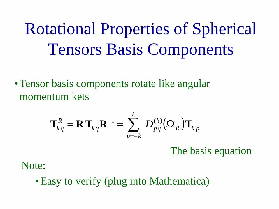
Rotational Properties of Spherical Tensors Basis Components
•Tensor basis components rotate like angular momentum kets
Note: •Easy to verify (plug into Mathematica)
( ) pkRkqp
k
kpqk
Rqk D TRTRT Ω== ∑
−=
− )(1
The basis equation

• Expansion of an arbitrary matrix
jkjk
k
kjkjkjk
k
kjkba TTA *
2
0
2
0∑∑∑∑
−==−==
==
AT†jkjkjk Trba == *
=
zzyzxz
zyyyxy
zxyxxx
aaaaaaaaa
A
• Bases not Hermitian, so
nlmknmlkTr δδ=TT†
STB: Complete and Orthonormal
Mehring“symmetric”
Mueller, CMR“direct”

STB: Complete and Orthonormal
• Not Hermitian, so use
nlmknmlkTr δδ=TT†
• Expansion of an arbitrary matrix
jkjk
k
kjka TA ∑∑
−==
=2
0
AT†jkjk Tra =
[ ][ ]
( )[ ]( )[ ]
( )[ ]( )[ ]xyyxyyxx
yzzyxzzx
zzyyxxzz
zyyzzxxz
xyyxi
zzyyxx
aaiaaa
aaiaaa
aaaaa
aaiaaa
aaa
aaaa
+−=
++=
++−=
−−−=
−=
++−=
±
±
±
21
22
21
12
61
02
21
11
201
31
00
3• Coefficients defined this way are
the complex conjugates of those frequently encountered in the literature (no fundamental problem).
=
zzyzxz
zyyyxy
zxyxxx
aaaaaaaaa
A

Rotation of Spherical Tensors
( )
( ) qkjkRkjq
k
kj
k
kqk
qkRkjq
k
kqjk
k
kjk
jkjk
k
kjk
aD
Da
a
T
T
RTR
RARA
Ω=
Ω=
=
=′
∑∑∑
∑∑∑
∑∑
−=−==
−=−==
−==
)(2
0
)(2
0
2
0
1-
-1

Rotation of Spherical Tensors( )
( ) ( ) ( )( ) ( ) ( )( ) ( ) ( )
( ) ( ) ( ) ( ) ( )( ) ( ) ( ) ( ) ( )( ) ( ) ( ) ( ) ( )( ) ( ) ( ) ( ) ( )( ) ( ) ( ) ( ) ( )
ΩΩΩΩΩΩΩΩΩΩΩΩΩΩΩΩΩΩΩΩΩΩΩΩΩ
=
′′′′′
ΩΩΩΩΩΩΩΩΩ
=
′′′
Ω=′
−
−
−−
−−
−−
−−−−−−−
−−−−−−−
−
−
−
−
−
−−−−−
22
12
02
12
22
)2(22
)2(12
)2(02
)2(12
)2(22
)2(21
)2(11
)2(01
)2(11
)2(21
)2(20
)2(10
)2(00
)2(10
)2(20
)2(21
)2(11
)2(01
)2(11
)2(21
)2(22
)2(12
)2(02
)2(12
)2(22
22
12
02
12
22
11
01
11
)1(11
)1(01
)1(11
)1(10
)1(00
)1(10
)1(11
)1(01
)1(11
11
01
11
00)0(
0000
aaaaa
DDDDDDDDDDDDDDDDDDDDDDDDD
aaaaa
aaa
DDDDDDDDD
aaa
aDa
RRRRR
RRRRR
RRRRR
RRRRR
RRRRR
RRR
RRR
RRR
R rank 0
rank 1
rank 2

The Secular Component
Typically just need to keep track of the secular component of the rotated tensor or the coefficient of the 2,0th
component of the rotated spherical tensor
zozz IH ωσ=secularCS,
( ) ( )γβασ
σσ
γβασσσσσσσσσ
,,00
0000
,, 1−
=
RR
ZZ
YY
XX
zzzyzx
yzyyyx
xzxyxx
0031
0232 σσσ −=zz

The “Coefficient” Equation
( ) ( ) ( ) ( ) ( )( ) ( ) ( ) ( ) ( )( ) ( ) ( ) ( ) ( )( ) ( ) ( ) ( ) ( )( ) ( ) ( ) ( ) ( )
ΩΩΩΩΩΩΩΩΩΩΩΩΩΩΩΩΩΩΩΩΩΩΩΩΩ
=
′′′′′
−
−
−−
−−
−−
−−−−−−−
−−−−−−−
−
−
22
12
02
12
22
)2(22
)2(12
)2(02
)2(12
)2(22
)2(21
)2(11
)2(01
)2(11
)2(21
)2(20
)2(10
)2(00
)2(10
)2(20
)2(21
)2(11
)2(01
)2(11
)2(21
)2(22
)2(12
)2(02
)2(12
)2(22
22
12
02
12
22
aaaaa
DDDDDDDDDDDDDDDDDDDDDDDDD
aaaaa
RRRRR
RRRRR
RRRRR
RRRRR
RRRRR
( ) pRpqp
q aDa 2)2(
2
22 Ω=′ ∑
−=
Tensor before the rotation of the physical system.
Tensor after the rotation of the physical system.

Rotated ComponentsThe basis “component” equation
The “coefficient” equation
Do not want to confuse these two equations!
( ) pRqpp
qRq D 2
)2(2
2
122 TRTRT Ω== ∑
−=
−
( ) pRpqp
q aDa 2)2(
2
22 Ω=′ ∑
−=
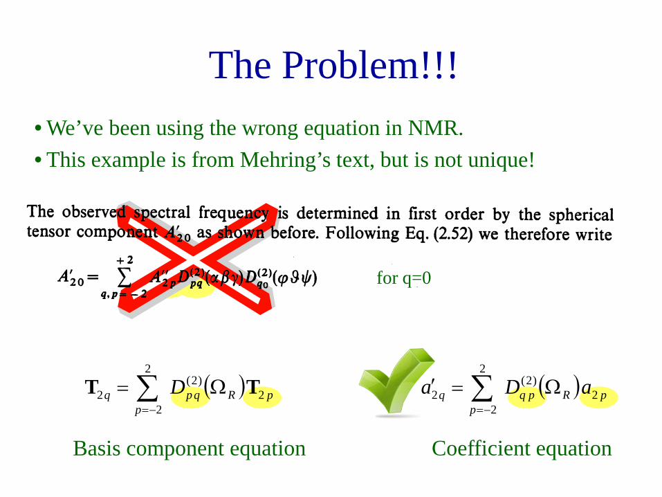
The Problem!!!
for q=0
• We’ve been using the wrong equation in NMR.• This example is from Mehring’s text, but is not unique!
( ) pRqpp
q D 2)2(
2
22 TT Ω= ∑
−=
Basis component equation Coefficient equation
( ) pRpqp
q aDa 2)2(
2
22 Ω=′ ∑
−=

• Expansion of an arbitrary matrix
jkjk
k
kjkb TA *
2
0∑∑
−==
=
AT†jkjk Trb =*
[ ][ ]
( )[ ]( )[ ]
( )[ ]( )[ ]xyyxyyxx
yzzyxzzx
zzyyxxzz
zyyzzxxz
xyyxi
zzyyxx
aaiaab
aaiaab
aaaab
aaiaab
aab
aaab
+±−=
+±+=
++−=
−±−−=
−−=
++−=
±
±
±
21
22
21
12
61
02
21
11
201
31
00
3
=
zzyzxz
zyyyxy
zxyxxx
aaaaaaaaa
A
• Bases not Hermitian, so
nlmknmlkTr δδ=TT†
STB: Complete and Orthonormal
( ) jkkj
jk bb −+−= 1*
• Verify by direct substitution
Mehringconvention

The Coefficient Equation
( ) *)(*pkR
kpq
k
kpqk bDb Ω=′ ∑
−=
( ) pkRkqp
k
kpqk bDb 1
)(−Ω=′ ∑
−=
( ) ( ) ( )1)(1)(*)(
−Ω=Ω=Ω −
RkqpR
kqpR
kpq DDD
( ) ( ) 1),(),( −Ω=Ω Rpassivek
qpRactivek
qp DD
Form I
Form II

Bases and CoefficientsThe basis equation
The coefficient equation
( ) pkRkqp
k
kpqk
Rqk D TRTRT Ω== ∑
−=
− )(1
( ) pkRkqp
k
kpkq bDb 1
)(−Ω=′ ∑
−=
( ) *)(*pkR
kpq
k
kpqk bDb Ω=′ ∑
−=

( ) pkRkqp
k
kpqk aDb 1
)(−Ω=′ ∑
−=( ) pkR
kqp
k
kpqk D TT Ω= ∑
−=
)(
The Problem!!!•We’ve been using the wrong equation in NMR.•This example is from Mehring’s text, but is not unique!
Basis equation Coefficient equation

An Example: Rotation of an AbInitio Chemical Shielding Tensor
−−−
−=
4.1198.21.50.50.1319.6
5.17.85.151aσ
−−−=
9.1207.71.39.100.1526.0
1.02.10.129I,bσ
Active rotation of molecule Cα CSA calculated in Gaussian (B3LYP, 6311++G**)

An Example: CS in Glycine
( ) ( )364A364AII ,,,, ππππππ -1RσRσ ab, =
−−−=
9.1208.71.39.100.1526.0
2.02.10.129II b,σ
Cartesian
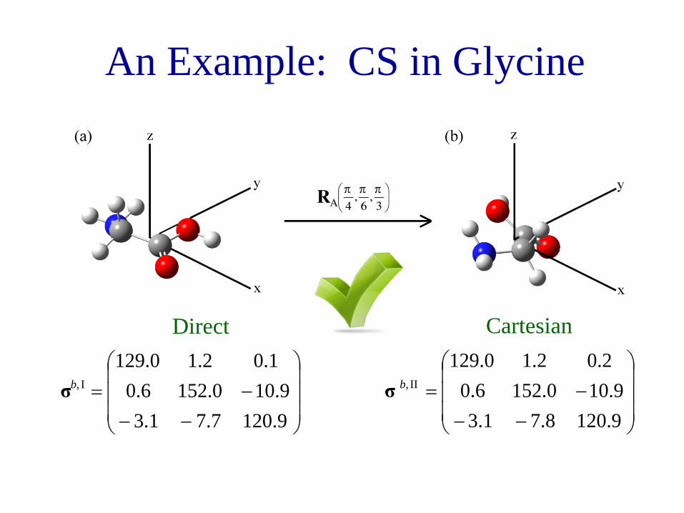
An Example: CS in Glycine
−−−=
9.1208.71.39.100.1526.0
2.02.10.129II b,σ
−−−=
9.1207.71.39.100.1526.0
1.02.10.129I b,σ
Direct Cartesian

An Example: CS in Glycine
1.
2.
3.
ajk
ajk Tr σT†=σ
( )( ) ajkR
kjq
k
kj
bqk D σσ πππ
364A ,,)( Ω= ∑
−=
−−−=
9.1208.71.39.100.1526.0
2.02.10.129III b,σ
jkb
jk
k
kjk
b, Tσ σ∑∑−==
=2
0
III
ST: Coefficient Eqn.

An Example: CS in Glycine
−−−=
9.1208.71.39.100.1526.0
2.02.10.129III b,σ
−−−=
9.1208.71.39.100.1526.0
2.02.10.129II b,σ
−−−=
9.1207.71.39.100.1526.0
1.02.10.129I b,σ
Direct
Cartesian
ST: Coefficient Eqn.
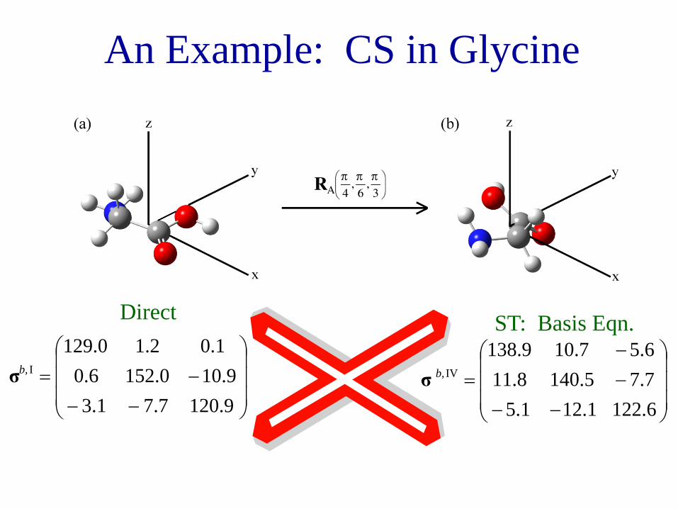
An Example: CS in Glycine
−−−−
=6.1221.121.57.75.1408.116.57.109.138
IV b,σ
−−−=
9.1207.71.39.100.1526.0
1.02.10.129I b,σ
Direct ST: Basis Eqn.

What Went Wrong?
• How come we did not notice this earlier?
• Compensating errors that appeared to make the approach consistent
- Used the basis equation - Switched the sense of rotation between the Cartesian and spherical tensor transformations

What Went Wrong?
• Mispairing of Cartesian and Wigner rotation matrices makes basis equation appear to work for coordinate transformations
• Not unique to Mehring’s text – predates use in NMR• Bouten, Physica 42 (1969) 572-580
• Errors in: Edmonds (1957), Rose (1957)• Correct in: Wigner (1959), Fano and Racah (1959), Edmonds (1996)
Passive!
Active!

Implications for NMR
Bad News:• You will read a lot of papers in which the rotations
implemented in spherical tensor form are the inverse of what was intended or stated

Implications for NMR
Good News:• You will read a lot of papers in which the rotations
implemented in spherical tensor form are JUST the inverse of what was intended or stated
Bad News:• You will read a lot of papers in which the rotations
implemented in spherical tensor form are the inverse of what was intended or stated
Implications for NMR
Simulation Programs:• Both Simpson and Spinach are in practice using the passive
convention
Good News:• You will read a lot of papers in which the rotations
implemented in spherical tensor form are JUST the inverse of what was intended or stated
Bad News:• You will read a lot of papers in which the rotations
implemented in spherical tensor form are the inverse of what was intended or stated

When Does it Matter?
• The consistent treatment of rotations of the physical system and spatial tensors in the NMR Hamiltonian is necessary to make connections back to the molecular frame
• The coordinate equation:
Mueller, Concepts in Magnetic Resonance A, 38A, 221-235 (2011)
( ) pkRkpq
k
kpqk aDa Ω=′ ∑
−=
)(

Hamiltonians in Spherical Tensor Form
=⊗=
zzyzxz
zyyyxy
zxyxxx
ISISISISISISISISIS
ISλλλ
λλλ
λλλ
λλS
[ ][ ]
( )[ ]( )[ ]
( )[ ]( )[ ]xyyxyyxx
yzzyxzzx
zzyyxxzz
zyyzzxxz
xyyxi
zzyyxx
ISISiISISs
ISISiISISs
ISISISISs
ISISiISISs
ISISs
ISISISs
+−=
++=
++−=
−−−=
−=
++−=
±
±
±
21
22
21
12
61
02
21
11
201
31
00
3
( ) jkjkj
k
kjk
jkjk
k
kjkjkjk
k
kjk
sac
sac
cSIcH
−−==
′′′′
′
′−=′=′−==
−=
=
=
⋅⋅=
∑∑
∑∑∑∑
1
Tr
Tr
2
0
2
0
2
0
λ
λ
λλλ
λλλλ
TT
SAA
An advantage of spherical tensors is that they isolate elements of 2nd
rank Cartesian tensors that transform together under rotation.
To take full advantage of them, must write the Hamiltonian in ST form

Secular Approximation[ ]
[ ]( )[ ]
( )[ ]( )[ ]
( )[ ]xyyxyyxx
yzzyxzzx
zzyyxxzz
zyyzzxxz
xyyxi
zzyyxx
ISISiISISs
ISISiISISs
ISISISISs
ISISiISISs
ISISs
ISISISs
+−=
++=
++−=
−−−=
−=
++−=
±
±
±
21
22
21
12
61
02
21
11
201
31
00
3
0
0
0
0
22
12
62
02
11
01
31
00
=
=
=
=
=
−=
±
±
±
s
s
ISs
s
s
ISs
zz
zz[ ]
( )[ ]
0
0
3
0
0
22
12
61
02
11
01
31
00
=
=
++−=
=
=
++−=
±
±
±
s
s
ISISISISs
s
s
ISISISs
zzyyxxzz
zzyyxx
• Discard terms that do not commute with IZ
tot
HeteronuclearHomonuclear
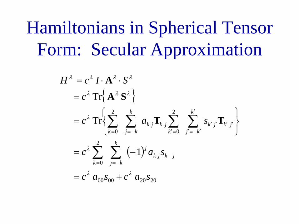
Hamiltonians in Spherical Tensor Form: Secular Approximation
( )
20200000
2
0
2
0
2
0
1
Tr
Tr
sacsac
sac
sac
cSIcH
jkjkj
k
kjk
jkjk
k
kjkjkjk
k
kjk
λλ
λ
λ
λλλ
λλλλ
+=
−=
=
=
⋅⋅=
−−==
′′′′
′
′−=′=′−==
∑∑
∑∑∑∑ TT
SAA

Hamiltonian and Reference Frames
( ) ( ) ( ) ( ) PASPAS
lab1labPAS
labPASPAS
lablabPAS
1PASlabPAS
lablab
SRARSA
SRARSA
ΩΩ==
ΩΩ==−
−
TrcTrc
TrcTrcHλλ
λλλ
( ) ( ) ( ) ( )
( ) ( ) ( ) ( ) labPAS
labPASPAS
lab1
PASlab
1labPASlab
PAS
labPAS
lablabPAS
1PAS
lablabPAS
1PASlabPAS
SRAR
RSRA
RSRA
SRAR
ΩΩ=
ΩΩ=
ΩΩ=
ΩΩ=
−
−
−
−
Trc
Trc
Trc
TrcH
λ
λ
λ
λλ
( )labPASΩR
Starting frame
Final frame
Trace is invariant with respect to basis, so can write the Hamiltonian in any reference frame
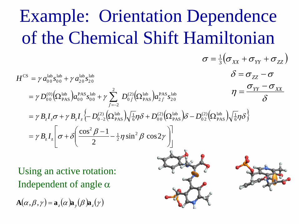
Example: Orientation Dependence of the Chemical Shift Hamiltonian
( ) ( )
( ) ( ) ( )
−
−+=
Ω−Ω+Ω−+=
Ω+Ω=
+=
−
′′−=′
∑
γβηβδσγ
ηδδηδγσγ
γγ
γγ
2cossin2
1cos 221
2
zz
61lab
PAS)2(
20labPAS
)2(006
1labPAS
)2(20
lab02
PAS2
labPAS
)2(0
2
2
lab00
PAS00
labPAS
)0(00
lab02
lab02
lab00
lab00
CS
IB
DDDIBIB
saDsaD
sasaH
zzzz
jjj
( )ZZYYXX σσσσ ++= 31
δσση XXYY −
=
σσδ −= ZZ
Using an active rotation:Independent of angle α
( ) ( ) ( ) ( )γβαγβα zyz aaaA =,,

Example: Hamiltonian under MAS
Part of problem set #1
( )[ ] ( )( )
( ) ( )( )γωβαηδ
γωβαηδ
γωβαηδ
γωβαηβδ
σγ
++
++−
++
++−+
−=
t
tt
t
IBH
r
r
r
r
zz
sincos2sin
cos2sin2cos122sincos2sin
22cos2cos12cossin
32
31
21
31
31
412
21
cs
0,,labrotor mrt θω=Ω
= −
31cos 1
mθ
Passive rotation• Angles describe how
to get from rotor back to lab frame
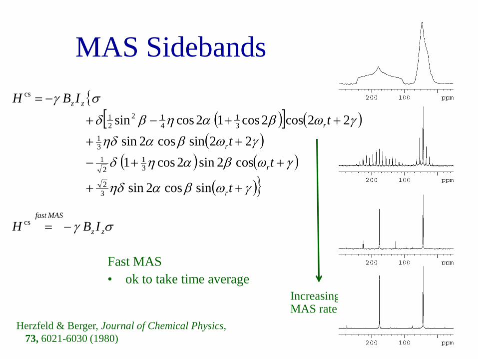
MAS Sidebands
( )[ ] ( )( )
( ) ( )( )γωβαηδ
γωβαηδγωβαηδ
γωβαηβδ
σγ
++
++−
++
++−+
−=
t
tt
tIBH
r
r
r
r
zz
sincos2sin
cos2sin2cos122sincos2sin
22cos2cos12cossin
32
31
21
31
31
412
21
cs
Increasing MAS rate
Herzfeld & Berger, Journal of Chemical Physics,73, 6021-6030 (1980)
σγ zz
MASfastIBH −=cs
Fast MAS• ok to take time average
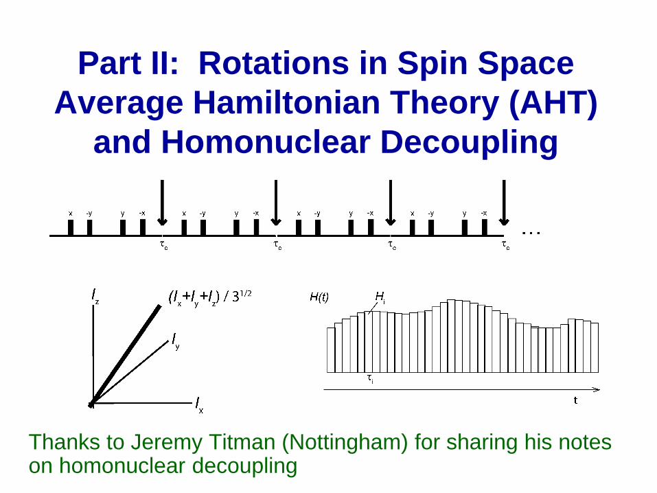
Part II: Rotations in Spin Space Average Hamiltonian Theory (AHT)
and Homonuclear Decoupling
Thanks to Jeremy Titman (Nottingham) for sharing his notes on homonuclear decoupling

Time Evolution and Average Hamiltonian Theory
( ) ∏ −=j
iH jjetU τ
( ) tHietU −=
∑≠j
jHH
[ ] 0, =kj HHunlessEffective Hamiltonian
• MAS and multiple pulses lead to time-dependent Hamiltonians
• Complicates dynamics when H does not always commute with itself at all times

Time-Dependent Problems in NMR
Several approaches exist:•Large term in Hamiltonian dominates
- Interaction representation •Periodic Hamiltonian with “small” terms
- Average Hamiltonian Theory•General Problem
- Brute force
( ) ∏ −=j
iH jjetU τ

The Rotating Frame:Preliminaries
( ) ( ) ( )ttiHtt ψψ −=∂∂
( ) ( ) ( )oo tttUt ψψ ,=
( ) ( ) ( )00 ,, ttUtiHttUt −=∂∂
( ) ( ) ( )[ ]ttHitt ρρ ,−=∂∂
( ) ( ) ( ) ( )oo ttUtttUt ,, 0+= ρρ
Equations of motion from Q.M. (always satisfied)

The Rotating FrameIn NMR the Zeeman interaction dominates when viewed from the lab frame
So pick a reference frame that rotates about the z-axis near the Larmor frequency from which to view the system.
( ) ( )tHHItH rfizio
i++= ∑ intω
Picture courtesy of Mei Hong

The Rotating FrameIn NMR the Zeeman interaction dominates when viewed from the lab frame
So pick a reference frame that rotates about the z-axis near the Larmor frequency from which to view the system.
Note this is a PASSIVE rotation! Coriolis force!
( ) ( )tHHItH rfizio
i++= ∑ intω
( ) totzIti
o etU ω=

The Rotating Frame: The Math( ) ( ) ( )ttUt o ψψ =~
( ) ( ) ( )oo tttUt ψψ ~,~~ =
( ) ( ) ( ) ( ) ( )ooooo ttUttUtUt ψψ ,~+=
( ) ( ) ( ) ( )( ) ( ) ( ) ( )ooooo
ooooo
tUttUtUttU
tUttUtUttU+
+
=
=
,,~,~,
( ) ( ) ( ) ( ) ( )o
eff
ooootot
ttUHi
tUttUtUttU
,~~,,~
−=
= +∂∂
∂∂
( ) ( ) ( ) ( ) ( ) ( ) ( )( ) ( ) ( ) ( ) ( ) ( ) ( )tUtUitHtUtUitHUtU
tUtiUtHtUtiUtHUtUH
oooooo
ooooooeff
+++
+++
+=+=
−=−=
~
~~
( ) ( )tUtU oto ∂∂= Time-evolution in the
rotating frame isn’t just due to Coriolis term!
( )tH~
Define rotating frame by Uo(t)
Time evolution in rot. frame
Substituting
Define rotating frame effective Hamiltonian

The Rotating Frame( ) tot
zItio etU ω=
( )
( ) ( )
( ) ( )tHtHI
tHtHI
etHHeI
IHeeH
rfzi
io
rfzi
io
Itirf
Itiz
i
io
totz
ItiItieff
totz
totz
totz
totz
secsecint
int
int
~~
~~
~
++∆≈
++∆=
++∆=
−=
∑
∑
∑ −
−
ω
ω
ω
ωωω
ωω
( ) ( )tHHItH rfizio
i++= ∑ intω
The secular approximation: Ignore terms with fast time-dependence
tItIeIe yxIti
xIti zz ωωωω sincos −=− Rotating at Larmor
frequency – ignore(left behind in lab frame)
Much smaller offset freqand may change t.d. of Hrf

Secular Approximation[ ]
[ ]( )[ ]
( )[ ]( )[ ]
( )[ ]xyyxyyxx
yzzyxzzx
zzyyxxzz
zyyzzxxz
xyyxi
zzyyxx
ISISiISISs
ISISiISISs
ISISISISs
ISISiISISs
ISISs
ISISISs
+−=
++=
++−=
−−−=
−=
++−=
±
±
±
21
22
21
12
61
02
21
11
201
31
00
3
0
0
0
0
22
12
62
02
11
01
31
00
=
=
=
=
=
−=
±
±
±
s
s
ISs
s
s
ISs
zz
zz[ ]
( )[ ]
0
0
3
0
0
22
12
61
02
11
01
31
00
=
=
++−=
=
=
++−=
±
±
±
s
s
ISISISISs
s
s
ISISISs
zzyyxxzz
zzyyxx
• Discard terms that do not commute with IZ
tot
HeteronuclearHomonuclear

The Interaction Representation
• Generalization of the rotating frame.
• Uo(t) can be any large term in the Hamiltonian
• Example, spin-locking fields, CP, and Lee-Goldberg decoupling

Chemical Shift Under Spin-Lock
Let:( ) xz IItH 1ωω +∆=
In the interaction frame:
( ) [ ]xo tIitU 1exp ω=
( )
( ) ( ) 0
sincos
~
11
11
1
11
11
≈
+∆=−+∆=
−=−
−
yz
xtIi
xztIi
xtIitIieff
ItItIeIIe
IetHeHxx
xx
ωωωωωω
ωωω
ωωChemical shifts do not evolve under spin lock

Dipolar Coupling Under Spin-Lock
( ) [ ] )(3 2112121 xxzzD IIIIIItH ++⋅−= ωωIn the interaction frame:
( ) [ ])(exp 211 xxo IItItU += ω
( )( ) ( )( ) ( ) ( )( )
( ) ( )
( ) 212121
21212123
21212123
2121211111
1
3
sincossincos3
~11
IIIIIIIIII
IIIIII
IIItItItItIetHeH
xxD
xxD
yyzzD
yzyzD
totx
tIitIieff totx
totx
⋅−−=
⋅−−⋅=
⋅−+=
⋅−++=−= −
ωω
ω
ωωωωωωωω
time average
scaled by -1/2 and rotated to be along x

The “Toggling” Frame•An interaction representation for multi-pulse sequences that pushes ahead with the applied pulses
•Often used to analyze multi-pulse homonucleardecoupling

Homonuclear Decoupling
•The use of rf pulses to average dipolar couplings
•Used to improve resolution in 1H and 19F NMR spectra by removing homonuclear couplings

Homogeneous 1H Network
• In solids, 1H lines are broad, even under moderate MAS
• Inhomogeneous part shifts energies of the Zeeman eigenstates
• Homogeneous part mixes degenerate states and causes line broadening. Flip-flop transitions lead to fluctuations of the state that interfere with MAS when νr < D
( )+−−+ +−=⋅−∝ 212121
212121 23 IIIIIIIIIIH zzzzD
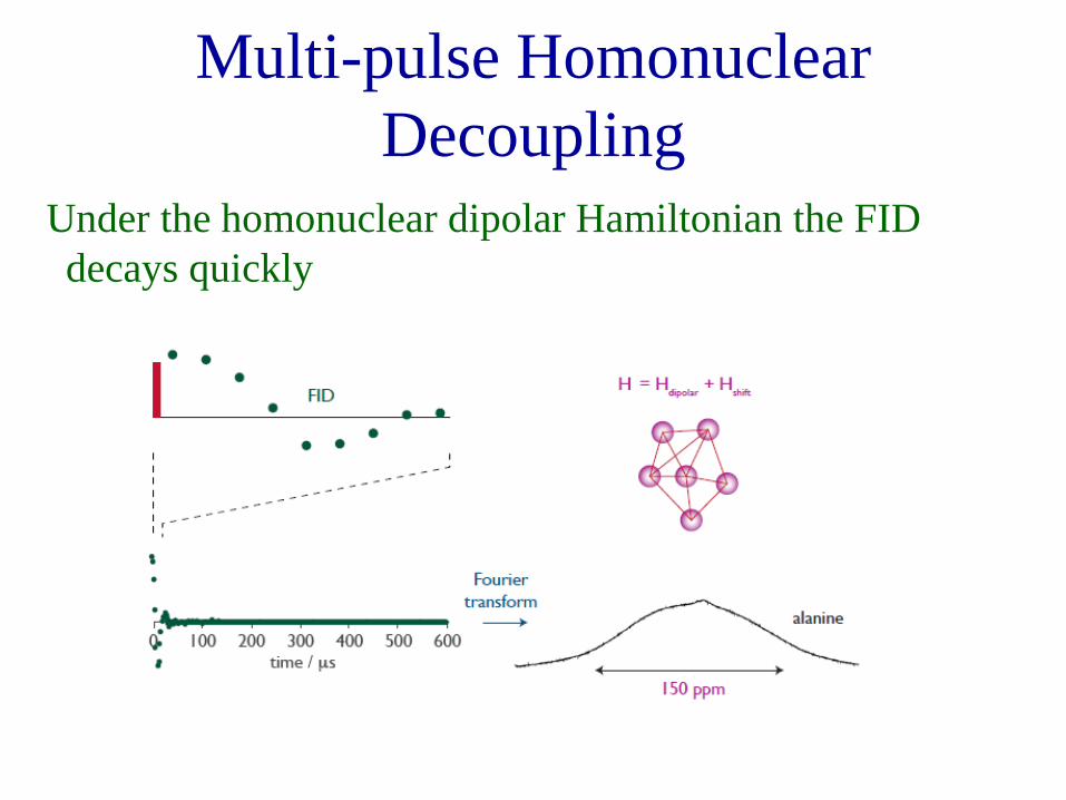
Multi-pulse HomonuclearDecoupling
Under the homonuclear dipolar Hamiltonian the FID decays quickly

Homonuclear decoupling involves sampling the FID stroboscopically, between bursts of a multi-pulse sequence designed to remove the dipolar interaction
Homonuclear Decoupling

Homonuclear Decoupling•Heteronuclear
( )zzIS
SID SIr
H 22
1cos3 2
3
−−=
βγγ ( )2121
2
312
2
32
1cos3 IIIIr
H zzD ⋅−
−−=
βγ
•Homonuclear
can independently flip not individually addressable

Homonuclear Decoupling
•WAHUHA
John Waugh

Average Hamiltonian Theory
Assuming :• A periodic Hamiltonian H(t) which is piecewise-constant over intervals τj
• Stroboscopic observation synchronized with the period of the Hamiltonian
Then it is possible to express the multi-pulse sequence as a transformation under an effective Hamiltonian given by the repeated application of the Baker-Campbell-Hausdorff expansion:
This expansion converges provided |Η|τc << 1Can also be applied to continuous pulses such as spin-locking fields
( ) ∑== jcjHtH ττ
[ ] [ ] [ ] ...,,,
...
1133223311222)1(
3322111)0(
)2()1()0(
+++=
+++=
+++=
− ττττττ
τττ
τ
τ
HHHHHHH
HHHHHHHH
c
c
i
eff

Calculating the Average Hamiltonian in the Toggling Frame
At the end of the cycle the toggling frame and rotating frame are back in register.

( )( )( )2121
2121
2121
333
IIIIDHIIIIDHIIIIDH
yyYY
xxXX
zzZZ
⋅−=
⋅−=
⋅−=
τττττ ππππ ZZx
ZZy
ZZy
ZZx
ZZ iHIiiHIiiHIiiHIiiH eeeeeeeeeU −−−−−−−= 2222 2
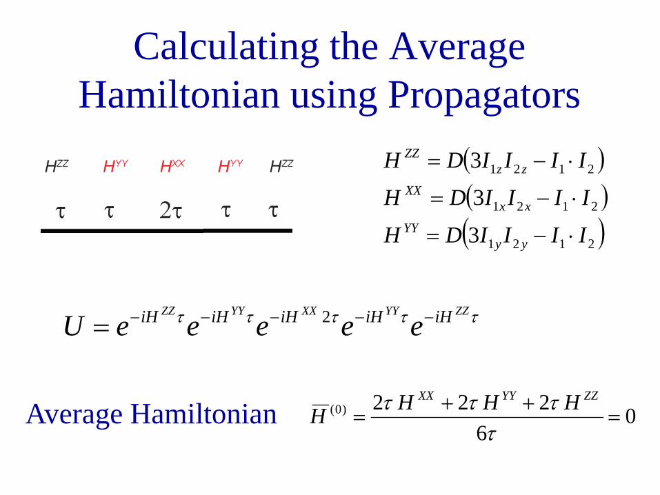
Calculating the Average Hamiltonian using Propagators
ττ ππ 22 22XX
yZZ
y iHIiiHIi eeee −−− =
τττττ ππ ZZx
ZZXXZZx
ZZ iHIiiHiHiHIiiH eeeeeeeU −−−−−−= 22 2
problem set #1

( )( )( )2121
2121
2121
333
IIIIDHIIIIDHIIIIDH
yyYY
xxXX
zzZZ
⋅−=
⋅−=
⋅−=
Calculating the Average Hamiltonian using Propagators
τττττ ππ ZZx
ZZXXZZx
ZZ iHIiiHiHiHIiiH eeeeeeeU −−−−−−= 22 2
( )( )( )2121
2121
2121
333
IIIIDHIIIIDHIIIIDH
yyYY
xxXX
zzZZ
⋅−=
⋅−=
⋅−=
Calculating the Average Hamiltonian using Propagators
τττττ ZZYYXXYYZZ iHiHiHiHiH eeeeeU −−−−−= 2
Average Hamiltonian 06
222)0( =++
=τ
τττ ZZYYXX HHHH

AHT: Chemical Shift Scaling
yY
xX
zZ
IHIHIH
ω
ω
ω
∆=
∆=
∆=
Average Hamiltonian is
( )zyx
ZYX
III
HHHH
++∆
=
++=
3
6222)0(
ωτ
τττ

WAHUHA
yY
xX
zZ
IHIHIH
ω
ω
ω
∆=
∆=
∆=
Average Hamiltonian is
( )33
6222)0(
zyx
ZYX
III
HHHH
++∆=
++=
ωτ
τττ
scaling factor = 0.577

WAHUHA
U. Haeberlen, U. Kohlschütter, J. Kempf, H.W. Spiess and H. Zimmerman, Chem. Phys., 3, 248 (1974).
τc short, ~ 20 µs

Improved Homonuclear DecouplingMuch effort has been expended modifying the basic sequence so that:• Higher order terms are removed from the effective Hamiltonian• Terms arising from rf inhomogeneity, pulse imperfections, and resonance
offsets are compensated
Symmetric Cycles: all odd-order terms cancel
Supercycles: MREV-8 repeats WAHUHA cycle with phase supercycle. Removes effect of rf inhomogeneity.
( ) ( )tHtH c −= τ

Combination with MASCRAMPS
• Combines spin-space averaging of a multi-pulse sequence with the spatial averaging of MAS
• Assumes the sample is static on the time scale of the multi-pulse sequence cycle time

Experimental AspectsSecond averaging: Homonuclear decoupling is most efficient when applied
off-resonance
Phase transients: The main pulse imperfections that cannot be easily compensated for with a supercycle. These can be minimized by detuning the probe/amplifier slightly.
Chemical shift scaling: Chemical shift evolution is about an effective field, so observed shifts are scaled. The scaling factor can be calculated, but is usually found empirically.

DUMBOReplaces multi-pulse sequence with a continuously phase-modulated rf pulse.
Theoretically only works in the CRAMPS regime (τc < τr), but practically it operates well with τc = 30 µs and νr = 25 kHz.
A. Lesage, D. Sakellariou, S. Hediger, B. Elena, P. Charmont, S. Seuernagel and L. Emsley, J. Magn. Reson., 163, 105 (2003).

Additional Sequences
T-MREVMSHOT-NTIMESFSLGPMLGand more!

Frequency-Switched Lee-Goldberg Decoupling
This method consists of a period of evolution about an effective field (the resultant of the resonance offset and the rf field B1) oriented at the magic angle and can be considered as a spin space variant of magic angle spinning.
Supercycles can be constructed by alternating periods of positive and negative offset frequency coupled with alternating B1 phase.
A. Bielecki, A. C. Kolbert and M. H. Levitt, Chem. Phys. Lett., 155, 341 (1989).

Conclusion
( ) jkjkj
k
kjksac
SIcH
−−==
−=
⋅⋅=
∑∑ 12
0
λ
λλλλ A

Ellipsoid Representation
Often represent tensors as ellipsoids with PAS components as axes. This is not a completely accurate mapping (but still useful). Correct shielding surface is given by an ovaloid.

Aside: Rotating (Wave)Functions
( ) ( ) ( )rrr
rrrRrrr11
11
''
''''
'
−−
−−
==
=====
=
RR
RR
R
ψψψψψψ
ψψ
• Same functional form but x’’,y’’,z’’ now depend on R and x,y,z.
y
x
Rψ(x,y)
ψ’(x,y)y’’
x’’
R-1• Best treated by
considering the inverse rotation of the coordinate system


![M. Billaud-Friess ,A.Nouyand O. Zahm€¦ · canonical tensors, Tucker tensors, Tensor Train tensors [27,40], Hierarchical Tucker tensors [25] or more general tree-based Hierarchical](https://img.pdfslide.us/doc/110x75/606a2ea8ed4bc80bc83876de/m-billaud-friess-anouyand-o-zahm-canonical-tensors-tucker-tensors-tensor-train.jpg)