Manifold Homotopy via the Flow Complex

Bardia Sadri∗

Abstract

It is known that the critical points of the distance function induced by a dense sample P ofa submanifold Σ of Rn are distributed into two groups, one lying close to Σ itself, called theshallow, and the other close to medial axis of Σ, called deep critical points. We prove that under(uniform) sampling assumption, the union of stable manifolds of the shallow critical points havethe same homotopy type as Σ itself and the union of the stable manifolds of the deep criticalpoints have the homotopy type of the complement of Σ. The separation of critical points underuniform sampling entails a separation in terms of distance of critical points to the sample. Thismeans that if a given sample is dense enough with respect to two or more submanifolds of Rn, thehomotopy types of all such submanifolds together with those of their complements are capturedas unions of stable manifolds of shallow versus those of deep critical points, in a filtration of theflow complex based on the distance of critical points to the sample. This results in an algorithmfor homotopic manifold reconstruction when the target dimension is unknown.

1 Introduction

Surface reconstruction is the problem of producing from a discrete sample of a surface Σ a conciselyrepresented surface Σ that closely approximates Σ and shares its topology, provided that the sampleis dense enough. Due to its many applications, this problem has a rich literature spanning severaldisciplines. In computational geometry a great deal of attention has been given to algorithms thatguarantee topological and geometric accuracy of the output under assumptions on the density ofthe sample; see e.g. [7, 3, 5, 4, 6, 2, 8, 9] or [13] for a survey. Traditionally, “topological equivalence”has been interpreted as homeomorphism or even the stronger notion of ambient isotopy. This inparticular requires the reconstructed object Σ to also be a manifold and of the same dimension asthe target surface Σ. In this paper, we relax this interpretation to homotopy equivalence (see [26] fordefinitions). Thus we seek to homotopically reconstruct the target manifold which consists of findinga concisely represented (here polyhedral) subset of Rn that is within small Hausdorff distance tothe original manifold and shares its homotopy type. We emphasize here that the outcome of ahomotopic reconstruction of a sampled manifold need not be a manifold itself.

An intuitive idea that has inspired several reconstruction algorithms [27, 1, 9] is to interpret thereconstructed surface as the zero level set of a (signed) distance function which evaluates to (near)zero in all of the sampled points. The distance function to the target surface itself is clearly one suchfunction. When the sample is sufficiently dense, the distance to the sample closely approximates thedistance to the target surface. Thus one may use the distance function induced by the sample as thestarting point for building the distance function that leads to the the reconstructed surface. Studyof distance functions as a natural approach to surface reconstruction has lead to the examination

∗Department of Computer Science, University of Toronto, Toronto, Ontario, Canada. The majority of work onthis paper was carried out when the author was at the University of Illinois at Urbana-Champaign.

1

of deeper properties of such functions such as their singularities, gradients, or steepest ascent flows[32, 20].

The flow complex was introduced by Giesen and John [22] as a tool for geometric modelingthough much of the mathematical foundations behind the flow complex were well-explored prior tothat (see [24] and references therein). In essence, for a discrete set P ⊂ Rn, the cells of the flowcomplex of P is a cell complex that partitions the entire space into a number of cells each of whichis a stable set (aka stable manifold) under a flow map φP that results from the integration of avector field vP that generalizes the gradient of the distance to P [28]. Each cell of the flow complexis the stable manifold of (set of all points that flow into) a critical point of the distance functioninduced by P . In [21], it was noted empirically that if P is a dense sample of a surface Σ, then theflow complex of P contains a subcomplex that approximates Σ.

Prior to [21], flow methods were employed for surface reconstruction (e.g. [20]) but the firstof such algorithms with geometric and topological guarantees was found by Dey et al. [18] whoproved a sharp separation of critical points of the distance function induced by surface samples intotwo groups. The points in the first group, called the shallow critical points lie close to the surfaceitself, and those in the second group, called the deep critical points lie close to the medial axis of thesurface. They further showed that for surfaces in R3, the boundary of the union of stable manifoldsof inner or outer deep critical points is homeomorphic to the original surface, provided that thesample is dense enough and meets extra regularity conditions.

Contributions. We prove important topological properties about the flow complex induced bydense samples of submanifolds of Rn of arbitrary dimension and codimension. These properties ina way generalize reconstruction result of [18], albeit with certain reservations. On the downside, westrengthen the adaptive sampling assumption of [18] to the uniform sampling where the sample is asubset of the manifold with bounded Hausdorff distance to it. Moreover, the notion of topologicalequivalence is weakened from homeomorphism to homotopy equivalence, thus our results translateto algorithms for homotopic reconstruction. On the upside, we prove that the union of stablemanifolds of the shallow critical points approximates the manifold and captures its homotopy typewhile that of the deep ones does the same for the complement of the manifold. Plus, we showthat this works for any closed submanifold of a Euclidean space of any dimension not just for(codimension-1) surfaces. Capturing the homotopy type of the complement in addition to thatof the manifold results in a much stronger topological guarantee. For example, all closed curves,knotted or not, have the same homotopy type and are in fact homeomorphic, but it is the homotopytypes of their complements that allow us to distinguish knotted curves from each other or from theunknotted ones. The homotopy equivalence of union of stable manifolds of shallow critical pointsto the target manifold simply follows from a sequence of known results on the homotopy types offlow shapes, alpha shapes, and union of balls [17, 29, 19, 11]. The other homotopy equivalence, i.e.between the union of stable manifolds of deep critical points and the complement of the manifold, isthe core result of this paper and its raison d’etre. Standard distance flow arguments as those usedin [28, 15, 23] fail in this case; see Section 5. We thus use a novel proof method that successivelyapplies such flow arguments on a family of intermediate sets that are indexed by the indices ofshallow critical points.

Rec

onst

ruct

ion

Usi

ng

Wit

nes

sC

omple

xes

Leo

nid

as

J.G

uib

as∗

Ste

ve

Y.O

udot†

Abst

ract

We

pre

sent

anov

elre

const

ruct

ion

alg

ori

thm

that,

giv

enan

input

poin

tse

tsa

mple

dfr

om

an

obje

ctS

,builds

aone-

para

met

erfa

mily

of

com

ple

xes

that

appro

xim

ate

Sat

dif-

fere

nt

scale

s.A

ta

hig

hle

vel

,our

met

hod

isver

ysi

milar

in

spir

itto

Chew

’ssu

rface

mes

hin

galg

ori

thm

,w

ith

one

nota

ble

diff

eren

ce:

the

rest

rict

edD

elaunay

tria

ngula

tion

isre

pla

ced

by

the

witnes

sco

mple

x,w

hic

hm

akes

our

alg

ori

thm

applica

-

ble

inany

met

ric

space

.To

pro

ve

its

corr

ectn

ess

on

curv

es

and

surf

ace

s,w

ehig

hlight

the

rela

tionsh

ipbet

wee

nth

ew

it-

nes

sco

mple

xand

the

rest

rict

edD

elaunay

tria

ngula

tion

in

2d

and

in3d.

Spec

ifica

lly,

we

pro

ve

that

both

com

ple

xes

are

equalin

2d

and

close

lyre

late

din

3d,

under

som

em

ild

sam

pling

ass

um

pti

ons.

1In

troducti

on

The

pro

ble

mof

reco

nst

ruct

ing

acu

rve

ora

surf

ace

from

scat

tere

ddat

apoi

nts

has

rece

ived

alo

tof

atte

nti

onin

the

pas

t.A

lthou

ghit

isill-pos

edin

gener

al,

since

in-

finit

ely

man

ysh

apes

wit

hdiff

eren

tto

pol

ogic

alty

pes

can

inte

rpol

ate

agi

ven

poi

nt

clou

d,

anum

ber

ofpro

vably

good

met

hods

hav

ebee

npro

pos

ed.

The

com

mon

de-

nom

inat

orof

thes

em

ethods

isth

eas

sum

pti

onth

atth

ein

put

poi

nt

set

isden

sely

sam

ple

dfr

oma

suffi

cien

tly

regu

lar

shap

e:th

isas

sum

pti

onm

akes

the

reco

nst

ruc-

tion

pro

ble

mw

ell-pose

d,

since

all

suffi

cien

tly

regu

lar

shap

esin

terp

olat

ing

the

poi

nt

set

hav

eth

esa

me

topo-

logi

calty

pe

and

are

clos

eto

one

anot

her

geom

etri

cally.

Itsu

ffice

sth

ento

appro

xim

ate

any

ofth

ese

shap

esto

get

the

righ

tan

swer

.T

he

noti

onofε-

sam

ple

,in

troduce

dby

Am

enta

and

Ber

n[1

],pro

vid

esa

sound

math

emat

ical

fram

ewor

kfo

rth

iskin

dof

appro

ach

,th

eco

rres

pon

din

gse

tof

reco

nst

ruct

ible

shap

esbei

ng

the

clas

sof

man

ifold

sw

ith

posi

tive

reach

[21]

.A

num

ber

ofpro

vably

-good

al-

gori

thm

sar

ebas

edon

the

ε-sa

mpling

theo

ry–

see

[7]fo

ra

surv

ey,an

dse

vera

lex

tensi

ons

hav

ebee

npro

pose

dto

reco

nst

ruct

man

ifol

ds

inhig

her

-dim

ensi

onal

spac

es[1

2]or

from

noi

sypoi

nt

clou

ddat

a[2

0].

The

theo

ryit

self

has

bee

nre

centl

yex

tended

toa

larg

ercl

ass

of

shap

es,

know

nas

the

clas

sof

Lip

schit

zm

anifol

ds[6

].In

all

thes

e

∗ Com

pute

rSci

ence

Dep

art

men

t,Sta

nfo

rdU

niv

ersi

ty.

guib

as@

cs.s

tanfo

rd.e

du

† Com

pute

rSci

ence

Dep

art

men

t,Sta

nfo

rdU

niv

ersi

ty.

stev

e.oudot@

stanfo

rd.e

du

met

hods,

the

Del

aunay

tria

ngula

tion

ofth

ein

put

poin

tse

tpla

ys

apro

min

ent

role

since

the

finalre

const

ruct

ion

isex

trac

ted

from

it.

Fig

ure

1:O

ne-

par

amet

erfa

mily

of

com

ple

xes

built

by

the

algo

rith

m,an

dth

eir

Bet

tinum

ber

s.

This

appro

ach

tosu

rfac

ere

const

ruct

ion

islim

ited

bec

ause

itas

sum

esim

plici

tely

that

apoi

ntcl

oud

shou

ldal

way

sre

pre

sent

asi

ngl

ecl

ass

of

shapes

.C

onsi

der

the

exam

ple

ofa

clos

edhel

icalcu

rve

rolled

around

ato

rus

inR

3–

see

Fig

ure

1.Tak

ea

very

den

seunifor

mpoi

nt

sam

ple

ofth

ecu

rve:

what

does

this

poin

tse

tre

pre

sent,

the

curv

eor

the

toru

s?A

lthough

bot

hob

ject

sar

ew

ell-sa

mple

dacc

ordin

gto

Am

enta

and

Ber

n’s

sam

pling

theo

ry,

clas

sica

lre

const

ruct

ion

met

hods

alw

ays

choose

asi

ngl

esh

ape,

her

eth

ecu

rve

orth

eto

rus,

by

rest

rict

ing

them

selv

esei

ther

toa

cert

ain

dim

ensi

onor

toa

cert

ain

scal

e:fo

rin

stance

,th

ere

const

ruct

ion

met

hod

of[1

2]or

the

dim

ensi

on

det

ecti

on

algo

rith

mof

[19]

willdet

ect

the

curv

ebut

not

the

toru

s,si

nce

the

poi

nt

set

isa

spar

sesa

mple

ofth

ecu

rve

but

not

ofth

eto

rus.

Now

,w

ecl

aim

that

the

resu

ltof

the

reco

nst

ruct

ion

should

not

be

eith

erth

ecu

rve

orth

eto

rus,

but

bot

hof

them

.M

ore

gener

ally,

the

resu

ltof

the

reco

nst

ruct

ion

shou

ldbe

aon

e-par

am

eter

fam

ily

ofco

mple

xes

,w

hose

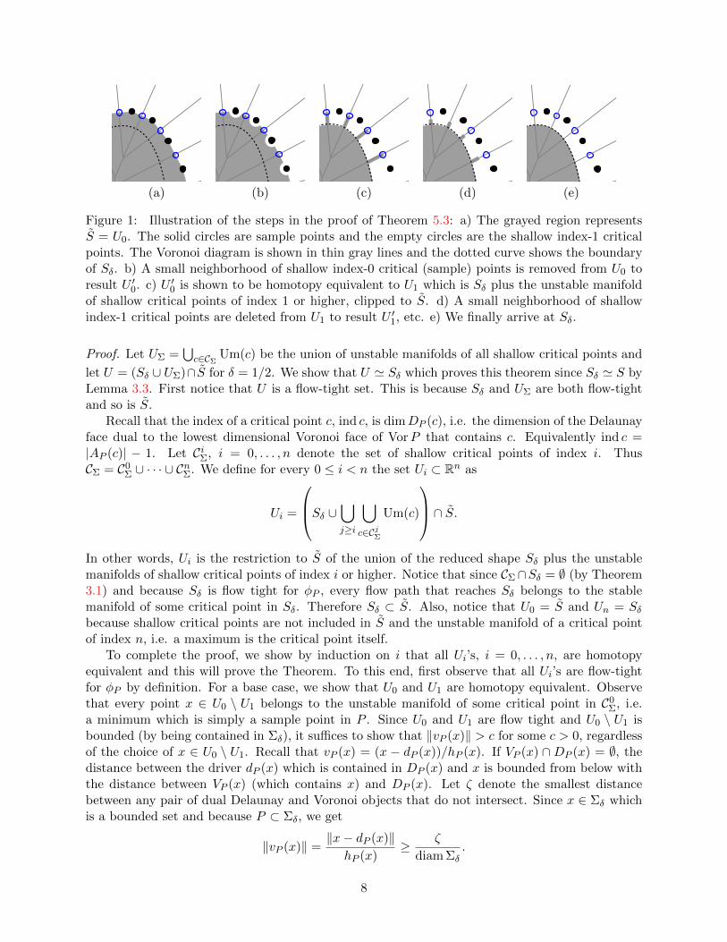
In many scientific settings, a subspace of interest from a high dimensional space isexpected to be a manifold or lie close to one. Naturally occurring data often have muchlower inherent dimension than the space in which they live. Inferring the topology ofsuch subspaces based on a collected sample poses a version of the manifold reconstruc-tion problem in which the dimension of the target manifold is not known. In fact, itcan be the case that the given sample is a dense sample for multiple submanifolds of

2

various dimensions of the larger space. For example, in the figure on the right, a sample of thecurve can also be regarded as a sample for the torus in which the curves is contained and given thesample alone as input, either the curve or the torus can be returned as a reconstruction of the targetmanifold. As a result, in recent years, there has been growing interest in manifold reconstructionalgorithms that are not supplied with a target dimension (See e.g. [25]).

For uniform samples, the separation of critical points, which is determined in terms of theirdistance from the target manifold, translates into a separation in terms of the distance from thesample itself. In other words, if one sorts the critical points in the order of their distance to thesample, the shallow critical points make a prefix of this ordering. Thus if one filters the flow complexby putting together the stable manifolds, i.e. cells associated to, critical points in all prefixes ofthis ordered sequence, one is guaranteed to reach in this filtration a shape homotopy equivalentto any manifold that is represented densely enough by the given sample. As mentioned above,the union of stable manifolds of the remaining critical points then captures the homotopy type ofthe complement of that manifold. Notice that this filtration is independent of the manifold andis simply a function of the given sample. Thus in the above example of the curve on the torus, ifthe given sample is dense for both the curve and the torus, the above filtration results homotopicreconstruction of both the curve and the torus, as well as their complements, in different stages.

Two important remarks are in order:

1. The significance of the results of this paper is primarily theoretical as in practice the flowcomplex is expensive to compute. Numerical issues can affect the structural accuracy of thiscomplex and its exact computation has only been implemented in R3 [12]. This is in contrastto much more robustly manageable and more efficiently computable structures such as offsetsurfaces, alpha-shapes, or witness complexes (See e.g. [16]). Nevertheless, distance functionshave been repeatedly used as the basis of many reconstruction algorithms and we believe thatthe stable manifolds of the flow induced by these functions capture much of the structure ofthese functions and elucidate their role in manifold reconstruction.

2. Although the results presented in this paper are stated for uniform noise-free samples ofsmooth submanifolds of Rn, they all generalize to considerably broader settings at the costof adjustments of constants: noisy (but uniform) samples can be accommodated using theresults of [15]. Furthermore, the assumption of the target shape being a smooth manifoldcan be dramatically relaxed to allow arbitrary compacts subsets of Rn with positive µ-reachin which case the sample can be taken as any finite (µ, κ)-approximation of the shape for anappropriate choice of κ (See [14] for the definitions as well as a more general separation result).We omit these generalizations from this manuscript and leave them for the full-version of thispaper.

The structure of the paper is as follows: In Section 2 we formally introduce the flow map φPinduced by a point set P as well as the resulting flow complex. In Section 3 we prove a slightlydifferent version of the critical points separation result of [18] for uniform samples of submanifoldsof Rn of arbitrary dimension. In Section 4 we show that the union of stable manifolds of theshallow critical points capture the homotopy type of the manifold. Then in Section 5 we prove thecorresponding result for the deep critical points and the complement of the manifold. Concludingremarks are provided in Section 6.

3

2 Background and Preliminaries

Let P be closed nonempty subset of Rn. The complement of P is the open set P c = Rn \ P .For any point x ∈ P c, let hP (x) = infy∈P ‖x − y‖ be the distance function defined by P and letAP (x) = {y ∈ P : ‖x− y‖ = hP (x)}.

While the distance function hP is not smooth, it induces a vector field vP over P c whichbehaves like the gradient of hP in the sense that vP (x) 6= 0 if and only if there is a unique directionof steepest ascent for hP at x in which case the direction of this steepest ascent is given by vP (x)(see [24] for more general statement and details). The vector vP (x) at a point x is characterized

by vP (x) = x−dP (x)hP (x) , where dP (x), called driver of x is the center of the smallest enclosing ball of

AP (x), or equivalently, the closest point in convAP (x), the convex hull of AP (x), to x. The criticalpoints of hP are those points x for which vP (x) = 0, or equivalently, x = dP (x) ∈ convAP (x).

Lieutier [28] proved that if P c is bounded, then Euler schemes defined by vP on P c uniformlyconverge and this results in a flow map φP : R+×P c → P c (where R+ is the set of non-negative reals)which he also proved to be continuous in both variables (in fact some of these results on distancefunctions were discovered earlier in higher generality on semi-concave functions [30]). Intuitively,φP (t, x) is the point y that is reached from following the vector field vP for time interval of lengtht, starting at x, by infinitesimal movements proportional to the magnitude of vP . The map φP hasthe classical properties of a flow map, namely φP (0, x) = x, φP (s+ t, x) = φP (s, φP (t, x)), and forany point x and any t ≥ 0, vP (φP (t, x)) is the right-derivative of φP (t, x). Lieutier also proved thathP along any flow orbit, i.e. t 7→ hP (φP (t, x)) is increasing and in addition satisfies

hP (φP (t, x)) = hP (x) +

∫ t

0‖vP (φP (τ, x))‖2dτ. (1)

The special case where P is finite is of particular interest to us and the rest of this section goesover special properties of the flow maps in this case. Let VorP and DelP respectively denote theVoronoi and Delaunay complexes induced by P . For any point x ∈ Rn, we represent by VP (x) thelowest dimensional face of VorP that contains x, and by DP (x) the face in DelP dual to VP (x).The set AP (x) is the vertex set of DP (x) and dP (x) becomes the closest point on DP (x) to x. Itcan be verified that all points in the relative interior of the same Voronoi face have the same driver.Since the affine hulls of a Voronoi face and its dual are orthogonal with total dimension n, theyintersect in exactly one point. Thus if VP (x) and DP (x) intersect, then this intersection consistsof a single critical point which is the driver of x. All critical points (except for the maximum atinfinity) are characterized the same way (as intersection points of duals). Following [22], we makea general position assumption that all pairs of Voronoi and Delaunay objects that are dual to andintersect each other, do so in their relative interiors. The index of a critical point c is defined asthe dimension of DP (c).

For a given flow map φP , the flow orbit of a regular point x, denoted φP (x) is defined asφP ([0,+∞), x). For a set T we use φP (T ) for

⋃x∈T φP (x). Notice that by this definition T ⊆ φP (T ).

For a critical point c of hP , the set of all points x whose flow orbit converges to c is called thestable manifold of c and denoted by Sm(c) = {x : φP (+∞, x) = c}. Although there is no flow outof a critical point c, we study the orbits of points very close to c. Some of these points flow into cwhile other flow away from it. We define the unstable manifold Um(c) of a critical point c, as theset of all points into which points arbitrarily close to c flow. Formally, Um(c) =

⋂ε>0 φP (B(c, ε)),

where B(c, ε) denotes the open ball of radius ε centered at c. In other words, the unstable manifoldof c consists of c and all the integral lines that start infinitesimally close to c.

Proposition 2.1 Let P be finite. For a critical point c of hP , Um(c) = φP (VP (c)).

4

A set T is said to be flow-tight for φP if φP (T ) = T . Stable and unstable manifolds of criticalpoints and their union and intersections are flow tight. Let CP be the set of critical points of hPinduced by P (including the critical point at infinity). The (stable) flow complex of P , denotedSfcP is the collection of stable manifolds of all critical points in CP . Generically, the cell associatedto an index k critical point is a topological open k-ball. Moreover, if for critical points c, c′ ∈ CP ,c ∈ ∂ Sm(c′), then Sm(c) ⊂ ∂ Sm(c′). The following lemma states an important structural propertyof the stable and unstable flow complex that follows from the correctness of the algorithms forcomputing these complexes [31, 10].

Lemma 2.2 If for c ∈ CP , ind c = k, then every critical point c′ ∈ ∂ Sm(c) has index less thank, provided that Sm(c) does not intersect the (n − k − 1)-skeleton of VorP . Under the sameassumption, if c ∈ ∂Um(c′), then ind c′ < ind c.

All but a measure-0 set of points P satisfy the requirement that Sm(c) must stay clear fromfaces of VorP of dimension n− k − 1 or smaller (see [31]).

Terminology. For the rest of this paper, by a manifold we refer to a C2-smooth closed submani-fold Σ of Rn of arbitrary codimension. The medial axis M(Σ) of Σ consists of points in space with2 or more closest points in Σ. The reach of Σ is the minimum distance of any point of M(Σ) toΣ. The C2-smoothness of Σ implies that its reach is strictly positive. Any point x 6∈ M(Σ), has aunique closest point x in Σ. The half-line bounded at x through x hits M(Σ) for the first time ata point x (or at infinity).

A point set P ⊂ Σ is a uniform ξ-sample of Σ if ∀x ∈ Σ ∃p ∈ P : ‖x − p‖ ≤ ξ. For a givenparameter r ≥ 0, the union of balls

⋃p∈P B(p, r) is denoted by B(r)(P ). The α-shape of P of

parameter r, denoted K(r)(P ) is the underlying space of restriction of DelP to B(r)(P ) (see [19]).The flow shape of P for parameter r, denoted F (r)(P ) is the union of stable manifolds of criticalpoints at distance ≤ r from P (see [17]).

3 Shallow versus deep critical points

For any point x ∈ Rn\(Σ∪M(Σ)) let µ(x) = ‖x− x‖. If x is at infinity, then µ(x) =∞. Otherwise,

the ratio 0 < ‖x−x‖‖x−x‖ < 1, is a relative measure of how close to Σ or M(Σ) the point x is. It turns out

[18, 15] that when a (possibly noisy) sample P of Σ satisfies some density requirements, then criticalpoints of hP are distributed, according to the above measure, into two distinguishable groups, onelying very close to Σ and the other to M(Σ). We state an essentially weaker version of the lemmathat is formulated for uniform samples. A proof can be found in the Appendix. Variants of thisresult for noisy samples, or for surfaces of positive µ-read can be found in [15] and [14].

Theorem 3.1 Let P be an ετ -sample of a manifold Σ of reach τ with ε ≤ 1/√

3. Then for everycritical point c of hP , either ‖c− c‖ ≤ ε2τ, or ‖c− c‖ ≥ (1− 2ε2)τ. In the former case we call c ashallow critical point and in the latter a deep critical point.

The following Corollary is a technical improvement of Proposition 7.1 in [15] or Lemma 3.3 in[29].

Corollary 3.2 Let P be an ετ -sample of a manifold Σ of reach τ with ε ≤ 1/√

3. Then, forevery shallow critical point c of hP , hP (c) ≤

√5/3 · ετ , and for every deep critical point c′ of hP ,

hP (c′) ≥ (1− 2ε2)τ .

5

Proof. Let c be a shallow critical point of hP and let λ = ‖c − c‖/τ . Since c is shallow, λ ≤ ε2.Since µ(c) ≥ τ , by Lemma A.1, hP (c) ≤ `(ε, λ)τ . Therefore

hP (c) ≤√λ2 + ε2(1 + λ) · τ ≤

√ε4 + ε2(1 + ε2) · τ

=√

1 + 2ε2 · ετ ≤√

5

3· ετ.

On the other hand, if c′ is a deep critical point, by Theorem 3.1, ‖c′− c′‖ ≥ µ(c′)−2ε2τ ≥ (1−2ε2)τ .The proof follows from the fact that hP (c′) ≥ ‖c′ − c′‖. �

For any 0 ≤ δ < 1, the δ-tubular neighborhood of a manifold Σ of reach τ is defined as the setΣδ = {x ∈ Rn : ‖x− x‖ ≤ δτ}. Notice that M(Σ) ⊂ Σc

δ.The following statement is classical. A proof is supplied in the Appendix for completeness.

Lemma 3.3 For any 0 ≤ δ < 1, cl Σcδ is homotopy equivalent to Σc. In fact, the former is a strong

deformation retract of the latter.

The following lemma is an adaptation of a similar lemma from [23] for uniforms samples. Theproof is provided in the Appendix.

Lemma 3.4 Let P be an ετ -sample of a manifold Σ of reach τ with ε ≤ 1/(1+√

2). Then, cl Σcδ is

flow-tight under the flow φP , for any ε2

1−ε < δ < 1− ε− ε2

1−ε . In particular this is true for δ = 1/2.

The above lemma implies that union of stable manifolds of shallow critical points is containedin Σδ for δ = ε2/(1− ε) thus providing the Hausdorff distance guarantee for our homotopic recon-structions. Alternatively, one can replace Σδ with a union of balls of an appropriately small radiuscentered at all sample points and show that the complement of the this union is flow tight underφP (See e.g. [15]).

4 Homotopy Type of the Manifold

In this section we show that in a dense enough sample of a submanifold of Rn, the union of stablemanifolds of the shallow critical points has the same homotopy type as the manifold itself. Thisstatement follows from the following sequence of results.

Lemma 4.1 [29] Let Σ be a manifold of reach τ and let P be an ετ -sample of Σ for any ε ≤12

√3/5. Then B(r)(P ) deformation retracts (and is in particular homotopy equivalent) to Σ, for

any 2ετ < r <√

3/5 · τ .

Lemma 4.2 [19] For any r ≥ 0, B(r)(P ) and the α-shape K(r)(P ) are homotopy equivalent.

Lemma 4.3 [17, 11] For any r, the flow shape F (r)(P ) and the α-shapes K(r)(P ) are homotopyequivalent.

Theorem 4.4 Let Σ be a manifold of reach τ and let P be an ετ -sample of Σ for ε ≤ 12

√3/5.

Then Σ is homotopy equivalent to the union U of stable manifolds of shallow critical points of hP .

Proof. For a critical point c of hP , by Corollary 3.2 hP (c) ≤√

5/3 · ετ if c is shallow and hP (c) ≥(1 − 2ε2)τ if c is deep. For ε < 1

2

√3/5 the latter bound is strictly greater than the former and

therefore there is a positive value r for which hP (c) < r for every shallow critical point c andhP (c′) > r for every deep critical point c′. Thus the flow shape F (r)(P ) is precisely the union ofstable manifolds of shallow critical points of hP with respect to Σ. Lemmas 4.1, 4.2, 4.3 now implythat this union is homotopy equivalent to Σ. �

6

5 Homotopy Type of the Complement of the Manifold

In this section we prove that the union of stable manifolds of deep critical points has the homotopytype of Σc using the continuity of the flow map φP . The technique is inspired from the work ofLieutier [28]. A proof can be found in [31] (Theorem 4.20, page 111).

Theorem 5.1 Let P be a finite set of points in Rn. If for sets Y ⊂ X ⊂ Rn, X and Y are bothflow-tight for φP , i.e. φP (X) = X and φP (Y ) = Y , and if X \Y is bounded, and, finally, if there isa constant c > 0 for which ‖vP (x)‖ ≥ c for all x ∈ X \ Y , then X and Y are homotopy equivalent.

A difficulty in using the above theorem is that φP is proven in [28] to be continuous on P c as longas it is a bounded set. This can be overcome by clipping the space with a very large ball, thusletting P0 = P ∪ Bc where B is a very large ball satisfying P ⊂ 1

5B. It can then be verified thatwithin 1

2B, φP and φP0 agree which is enough for what we want to prove. In the sequel CΣ denotesthe set of shallow critical points of P where P is an ετ -sample of a manifold Σ of reach τ . Thevalue of ε is determined later. For shorthand, we write S for Σc as well Sδ for Σc

δ.

Lemma 5.2 Let c be a critical point of hP and let U ⊆ Rn be a flow-tight set for φP with c 6∈ U .Let V = rel intVP (c). For r ≥ 0, let Vr = V ∩ B(c, r). Then for every r ≥ 0, if U ∩ B(c, r) ⊂ V ,then U \ Vr is flow-tight for φP and U and U \ Vr have the same homotopy type.

Proof. We build a deformation retraction from U to U \ Vr. Since c is a critical point and V is therelative interior of the lowest-dimensional Voronoi face that contains c, c is the driver of the pointsin V . Consequently, if x 6= c is a point in V ∩ U , dP (x) = c and since U is flow-tight for φP , wehave

{x+ t(x− c) : t ≥ 0} ∩ clV ⊆ U.

Now, define the map ρr : Vr → ∂Vr (where ∂Vr is defined relative to the affine hull of Vr) asρr(x) = x + t(x − c) for the smallest t ≥ 0 such that ρr(x) ∈ ∂Vr. In other words, ρr(x) is thepoint at which the ray shot from x in the direction x − c hits the boundary of Vr. Since Vr isconvex (it is the intersection of V and B(c, r) which are both convex), it is easy to see that themap ρr is continuous (it is a central projection from a point in a convex set to the boundary of theconvex set) and because of the assumption that U ∩ B(c, r) ⊂ V this implies that the retractionmap ρ∗r : U → U \ Vr defined below is also continuous.

ρ∗r(x) =

{ρr(x) x ∈ Vr,x x ∈ U \ Vr.

We now define the map Rr : [0, 1]× U → U as

Rr(t, x) =

{(1− t)x+ tρr(x) x ∈ Vr,x x ∈ U \ Vr.

which gives us a straight line homotopy from the identity map of U to the retraction ρr.If U ∩B(c, r) ⊂ V , then for any y ∈ Vr ∩ U , only points in Vr can flow into y. In other words,

y = φP (t, x) for some t ≥ 0 and x ∈ U implies that x ∈ Vr. Therefore, all flow lines that areaffected by removal of Vr from U start in Vr. But we saw above that each such flow line loses aninitial segment in U \ Vr. Thus U \ Vr is flow tight for φP . �

Theorem 5.3 Let ε ≤ 12

√3/5. Let S =

⋃c∈C\CΣ Sm(c) be the union of stable manifolds of all

deep critical points of hP with respect to Σ. Then S is homotopy equivalent to S.

7

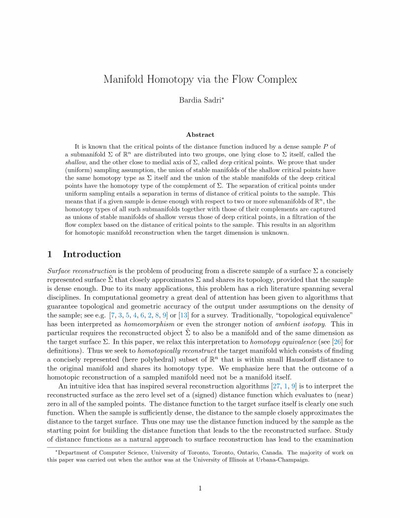
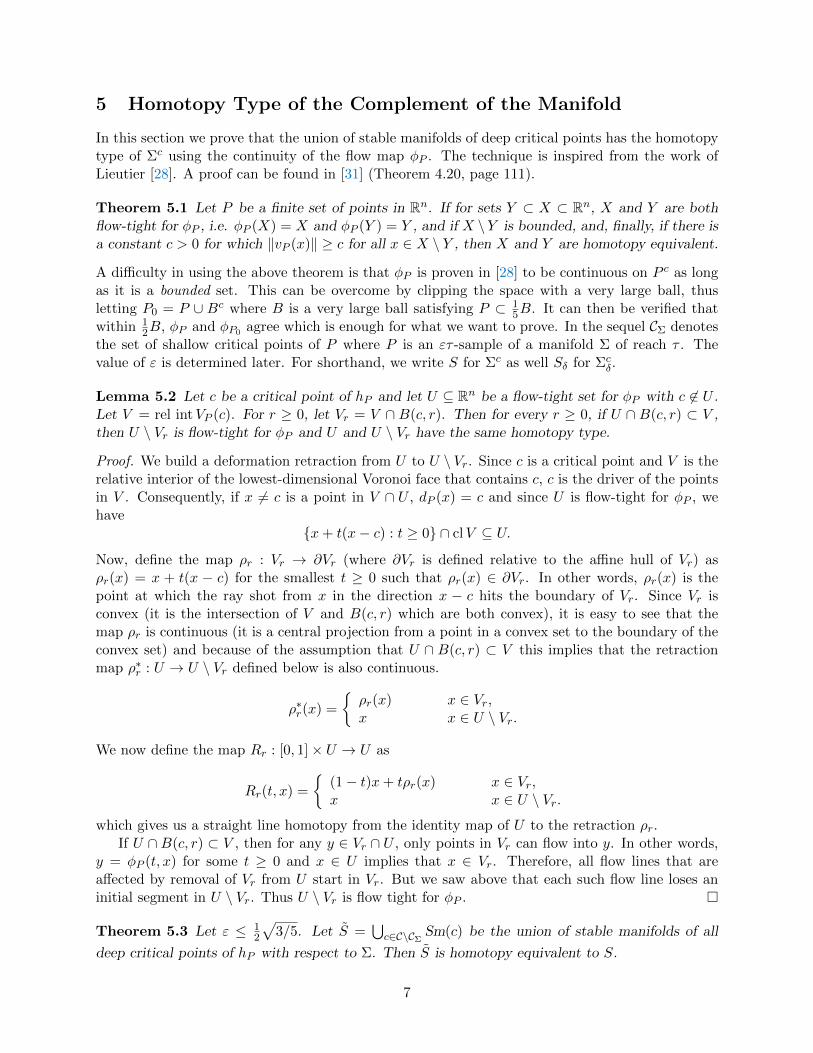
(a) (b) (c) (d) (e)

Figure 1: Illustration of the steps in the proof of Theorem 5.3: a) The grayed region representsS = U0. The solid circles are sample points and the empty circles are the shallow index-1 criticalpoints. The Voronoi diagram is shown in thin gray lines and the dotted curve shows the boundaryof Sδ. b) A small neighborhood of shallow index-0 critical (sample) points is removed from U0 toresult U ′0. c) U ′0 is shown to be homotopy equivalent to U1 which is Sδ plus the unstable manifoldof shallow critical points of index 1 or higher, clipped to S. d) A small neighborhood of shallowindex-1 critical points are deleted from U1 to result U ′1, etc. e) We finally arrive at Sδ.

Proof. Let UΣ =⋃c∈CΣ Um(c) be the union of unstable manifolds of all shallow critical points and

let U = (Sδ ∪ UΣ)∩ S for δ = 1/2. We show that U ' Sδ which proves this theorem since Sδ ' S byLemma 3.3. First notice that U is a flow-tight set. This is because Sδ and UΣ are both flow-tightand so is S.

Recall that the index of a critical point c, ind c, is dimDP (c), i.e. the dimension of the Delaunayface dual to the lowest dimensional Voronoi face of VorP that contains c. Equivalently ind c =|AP (c)| − 1. Let CiΣ, i = 0, . . . , n denote the set of shallow critical points of index i. ThusCΣ = C0

Σ ∪ · · · ∪ CnΣ. We define for every 0 ≤ i < n the set Ui ⊂ Rn as

Ui =

Sδ ∪⋃j≥i

⋃c∈CjΣ

Um(c)

∩ S.In other words, Ui is the restriction to S of the union of the reduced shape Sδ plus the unstablemanifolds of shallow critical points of index i or higher. Notice that since CΣ∩Sδ = ∅ (by Theorem3.1) and because Sδ is flow tight for φP , every flow path that reaches Sδ belongs to the stablemanifold of some critical point in Sδ. Therefore Sδ ⊂ S. Also, notice that U0 = S and Un = Sδbecause shallow critical points are not included in S and the unstable manifold of a critical pointof index n, i.e. a maximum is the critical point itself.

To complete the proof, we show by induction on i that all Ui’s, i = 0, . . . , n, are homotopyequivalent and this will prove the Theorem. To this end, first observe that all Ui’s are flow-tightfor φP by definition. For a base case, we show that U0 and U1 are homotopy equivalent. Observethat every point x ∈ U0 \ U1 belongs to the unstable manifold of some critical point in C0

Σ, i.e.a minimum which is simply a sample point in P . Since U0 and U1 are flow tight and U0 \ U1 isbounded (by being contained in Σδ), it suffices to show that ‖vP (x)‖ > c for some c > 0, regardlessof the choice of x ∈ U0 \ U1. Recall that vP (x) = (x − dP (x))/hP (x). If VP (x) ∩DP (x) = ∅, thedistance between the driver dP (x) which is contained in DP (x) and x is bounded from below withthe distance between VP (x) (which contains x) and DP (x). Let ζ denote the smallest distancebetween any pair of dual Delaunay and Voronoi objects that do not intersect. Since x ∈ Σδ whichis a bounded set and because P ⊂ Σδ, we get

‖vP (x)‖ =‖x− dP (x)‖

hP (x)≥ ζ

diam Σδ.

8

If, on the other hand, VP (x) ∩ DP (x) = {c}, then x ∈ Um(c). Since x ∈ U0 \ U1, c has to haveindex 0 and therefore c = dP (x) and ‖vP (x)‖ = 1.

Thus we assume that U0 ' · · · ' Ui and prove that Ui ' Ui+1. We do this in two stages. Firstwe construct a set U ′i by removing a neighborhood of every index-i shallow critical point in sucha way that U ′i is still flow tight for φP . We then show that Ui ' U ′i ' Ui+1 (See Figure 1). Theconstruction of U ′i uses Lemma 5.2. We thus remove for each shallow critical point c a neighborhoodB(c, rc) from Ui for which rc > 0 is chosen small enough so that B(c, rc) ∩ Ui ⊂ VP (c). This is thecase unless the unstable manifold of some other shallow critical point c′ reaches arbitrarily closeto c and is not contained in Um(c). Lemma 2.2 now implies that in this case ind c′ < ind c. Butthe unstable manifolds of shallow critical points of index less than i = ind c are not included in Ui.Thus by Lemma 5.2 we can remove a neighborhood of every shallow critical point of index i fromUi to get a set U ′i that is flow-tight for φP and is homotopy equivalent to U0.

Next we show that U ′i ' Ui+1. For this we use Theorem 5.1. Since U ′i and Ui+1 are bothflow-tight for φP , all we need to do is to find a lower bound for ‖vP (x)‖ for points x ∈ U ′i \ Ui+1.For any such point x, the driver dP (x) is contained in DP (x). There are two cases to consider;depending on whether VP (x) and DP (x) intersect or not.

If VP (x)∩DP (x) = ∅ then as argued above ‖vP (x)‖ ≥ ζ/(diam Σδ). On the other hand if VP (x)and DP (x) do intersect, their intersection will (by definition) be a critical point c which coincideswith dP (x). In this case x ∈ Um(c).

Notice that c cannot be a deep critical point since these critical points and their unstablemanifolds are contained in S1−2ε2 ⊂ Sδ which is flow-tight for φP . Thus c is a shallow criticalpoint. But in that case c must have index ≤ i since unstable manifolds of shallow critical points ofindex i+ 1 and higher are included in Ui+1 while c ∈ U ′i \ Ui+1. Therefore

‖vP (x)‖ =‖x− c‖hP (x)

≥dist(U ′i ,

⋃ij=0 C

jΣ)

diam Σδ> 0.

Theorem 5.1 now implies that U ′i ' Ui+1. The proof follows from the observation that Σδ ⊂ UΣ

and therefore S ⊂ Sδ ∪ UΣ implying that U = S. �The following corollary immediately follows from Corollary 3.1, Theorem 4.4, and Theorem

5.3. In essence, it enables us to reconstruct all the manifold a given sample densely represents (seeFigure 2).

Corollary 5.4 Let Σ1, . . . ,Σs be manifolds of various dimensions for all of which the same sampleP is an ετi-sample where τi is the reach of Σi, i = 1, . . . , s. If c1, . . . , cm are the set of criticalpoints of hP ordered such that hP (c1) < · · · < hP (cm), then for each i, there is a ji such that⋃j≤ji Sm(cj) ' Σi and

⋃j>ji

Sm(cj) ' Σci .

6 Conclusions

In this paper, we proved that the separation of critical points of a smooth submanifold of Rn leads toa very natural way of homotopic reconstruction of the submanifold and its complement. Combinedwith the fact that this separation can be formulated in terms of the distance from the sample, oneobtains a way of homotopic reconstruction of all submanifolds that are represented densely enoughby the input sample.

The main result of this paper generalizes to allow noisy samples, i.e. discrete point sets whichare within a small enough Hausdorff distance of the manifold. Using the original separation result of

9

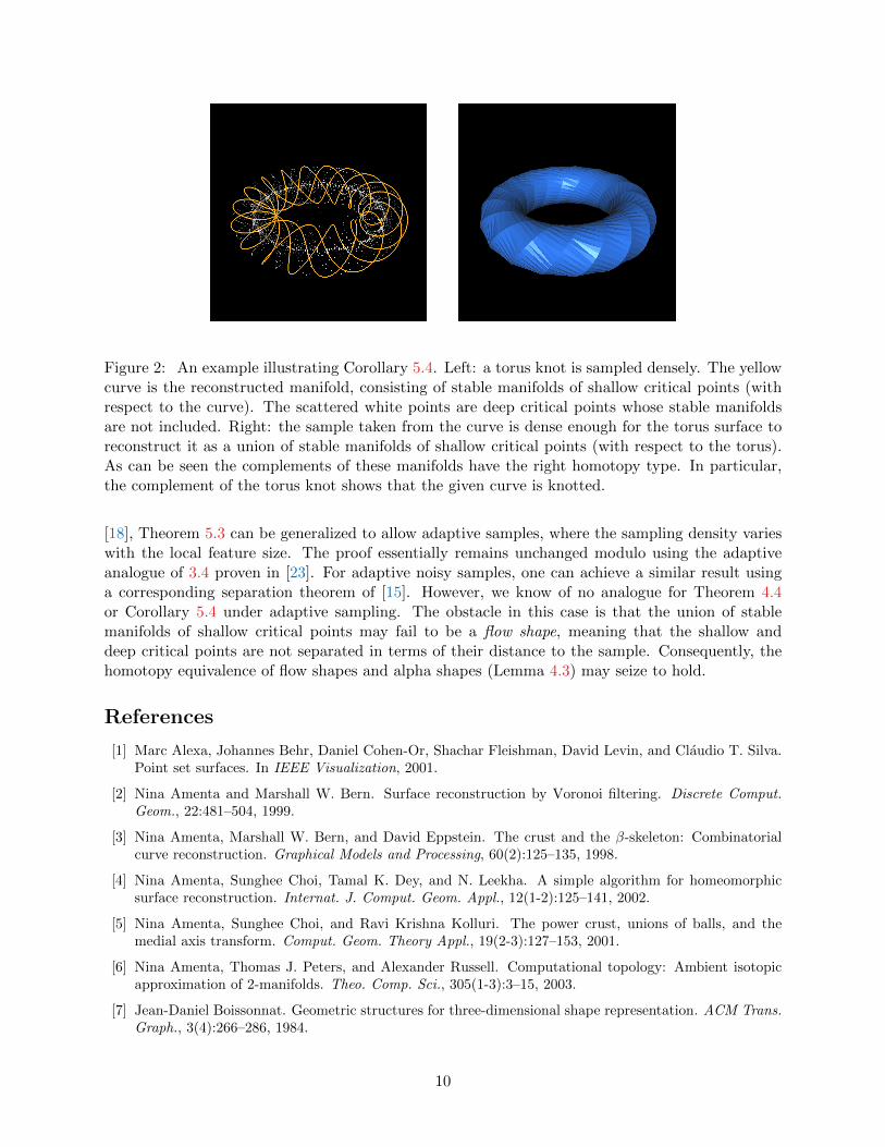
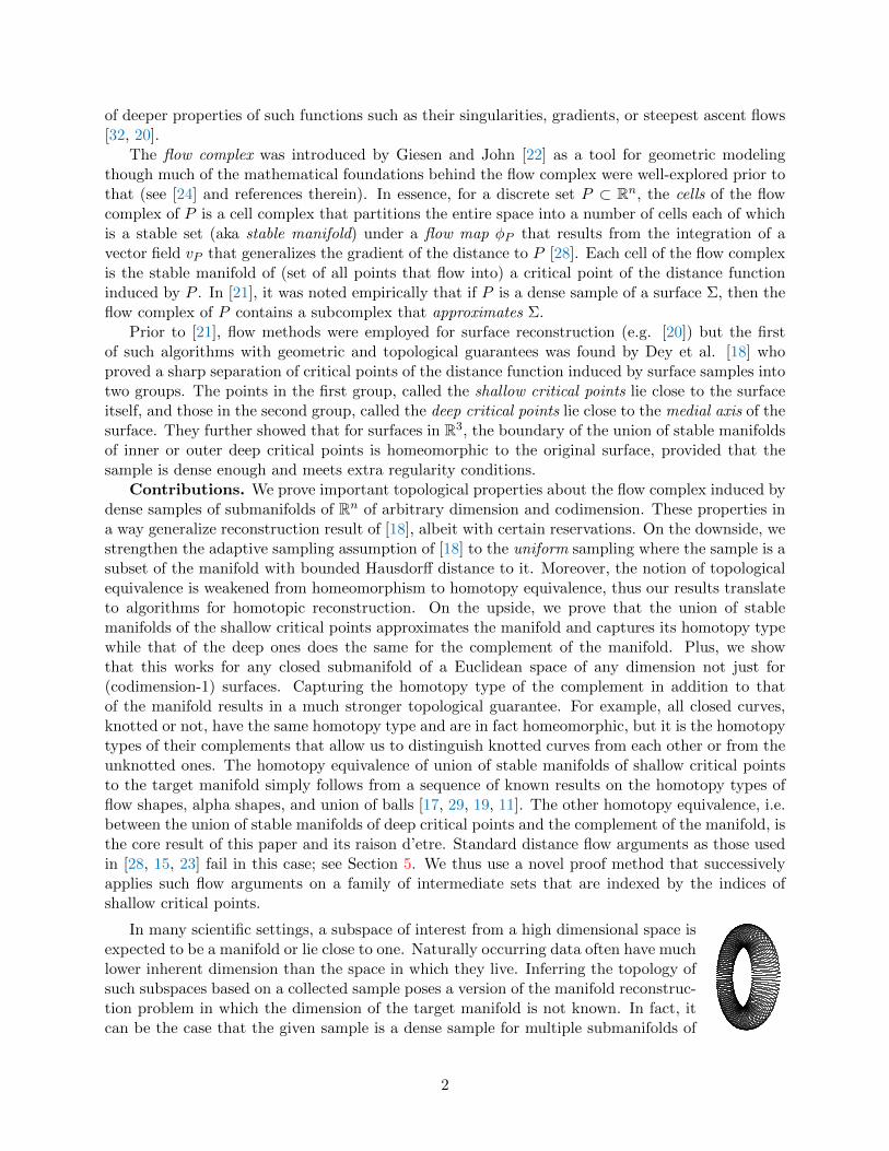
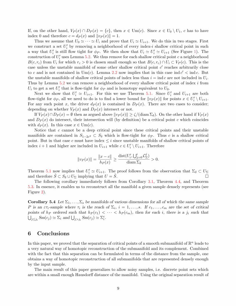
Figure 2: An example illustrating Corollary 5.4. Left: a torus knot is sampled densely. The yellowcurve is the reconstructed manifold, consisting of stable manifolds of shallow critical points (withrespect to the curve). The scattered white points are deep critical points whose stable manifoldsare not included. Right: the sample taken from the curve is dense enough for the torus surface toreconstruct it as a union of stable manifolds of shallow critical points (with respect to the torus).As can be seen the complements of these manifolds have the right homotopy type. In particular,the complement of the torus knot shows that the given curve is knotted.

[18], Theorem 5.3 can be generalized to allow adaptive samples, where the sampling density varieswith the local feature size. The proof essentially remains unchanged modulo using the adaptiveanalogue of 3.4 proven in [23]. For adaptive noisy samples, one can achieve a similar result usinga corresponding separation theorem of [15]. However, we know of no analogue for Theorem 4.4or Corollary 5.4 under adaptive sampling. The obstacle in this case is that the union of stablemanifolds of shallow critical points may fail to be a flow shape, meaning that the shallow anddeep critical points are not separated in terms of their distance to the sample. Consequently, thehomotopy equivalence of flow shapes and alpha shapes (Lemma 4.3) may seize to hold.

References

[1] Marc Alexa, Johannes Behr, Daniel Cohen-Or, Shachar Fleishman, David Levin, and Claudio T. Silva.Point set surfaces. In IEEE Visualization, 2001.

[2] Nina Amenta and Marshall W. Bern. Surface reconstruction by Voronoi filtering. Discrete Comput.Geom., 22:481–504, 1999.

[3] Nina Amenta, Marshall W. Bern, and David Eppstein. The crust and the β-skeleton: Combinatorialcurve reconstruction. Graphical Models and Processing, 60(2):125–135, 1998.

[4] Nina Amenta, Sunghee Choi, Tamal K. Dey, and N. Leekha. A simple algorithm for homeomorphicsurface reconstruction. Internat. J. Comput. Geom. Appl., 12(1-2):125–141, 2002.

[5] Nina Amenta, Sunghee Choi, and Ravi Krishna Kolluri. The power crust, unions of balls, and themedial axis transform. Comput. Geom. Theory Appl., 19(2-3):127–153, 2001.

[6] Nina Amenta, Thomas J. Peters, and Alexander Russell. Computational topology: Ambient isotopicapproximation of 2-manifolds. Theo. Comp. Sci., 305(1-3):3–15, 2003.

[7] Jean-Daniel Boissonnat. Geometric structures for three-dimensional shape representation. ACM Trans.Graph., 3(4):266–286, 1984.

10

[8] Jean-Daniel Boissonnat and Frederic Cazals. Smooth surface reconstruction via natural neighbourinterpolation of distance functions. Comput. Geom. Theory Appl., 22(1-3):185–203, 2002.

[9] Jean-Daniel Boissonnat and Steve Oudot. Provably good sampling and meshing of Lipschitz surfaces.In Proc. 22nd Annu. ACM Sympos. Comput. Geom., pages 337–346, 2006.

[10] Kevin Buchin, Tamal K. Dey, Joachim Giesen, and Matthias John and. Recursive geometry of the flowcomplex and topology of the flow complex filtration. Comput. Geom. Theory Appl., 40:115–157, 2008.

[11] Kevin Buchin and Joachim Giesen. Flow complex: General structure and algorithms. In Proc. 16thCanad. Conf. Comput. Geom., pages 270–273, 2005.

[12] Frederic Cazals. Robust construction of the extended three-dimensional flow complex. Research Report5903, INRIA, 2006.

[13] Frederic Cazals and Joachim Giesen. Delaunay triangulation based surface reconstruction. In Jean-Daniel Boissonnat and Monique Teillaud, editors, Effective Computational Geometry for Curves andSurfaces. Springer-Verlag, 2006.

[14] Frederic Chazal, David Cohen-Steiner, and Andre Lieutier. A sampling theory for compacts in Euclideanspace. In Proc. 22nd Annu. ACM Sympos. Comput. Geom., pages 319–326, 2006.

[15] Frederic Chazal and Andre Lieutier. Topology guaranteeing manifold reconstruction using distancefunction to noisy data. In Proc. 22nd Annu. ACM Sympos. Comput. Geom., pages 112–118, 2006.

[16] Frederic Chazal and Steve Yann Oudot. Towards persistence-based reconstruction in euclidean spaces.In SCG ’08: Proceedings of the twenty-fourth annual symposium on Computational geometry, pages232–241, 2008.

[17] Tamal K. Dey, Joachim Giesen, and Matthias John. Alpha-shapes and flow shapes are homotopyequivalent. In Proc. 35th Annu. ACM Sympos. Theory Comput., pages 493–502, 2003.

[18] Tamal K. Dey, Joachim Giesen, Edgar A. Ramos, and Bardia Sadri. Critical points of the distance toan epsilon-sampling of a surface and flow-complex-based surface reconstruction. In Proc. 21st Annu.ACM Sympos. Comput. Geom., pages 218–227, 2005.

[19] H. Edelsbrunner. The union of balls and its dual shape. Discrete Comput. Geom., 13:415–440, 1995.

[20] Herbert Edelsbrunner. Surface reconstruction by wrapping finite point sets in space. Discrete & Com-putational Geometry, 32:231–244, 2004.

[21] Joachim Giesen and Matthias John. Surface reconstruction based on a dynamical system. ComputerGraphics Forume, 21:363–371, 2002.

[22] Joachim Giesen and Matthias John. The flow complex: A data structure for geometric modeling. InProc. 14th ACM-SIAM Sympos. Discrete Algorithms, pages 285–294, 2003.

[23] Joachim Giesen, Edgar A. Ramos, and Bardia Sadri. Medial axis approximation and unstable flowcomplex. In Proc. 22nd Annu. ACM Sympos. Comput. Geom., pages 327 – 336, 2006.

[24] Karl Grove. Critical point theory for distance functions. Symposia in Pure Mathematics, 54(3):357–385,1993.

[25] Leonidas J. Guibas and Steve Oudot. Reconstruction using witness complexes. In Proc. 18th ACM-SIAM Sympos. Discrete Algorithms, pages 1076–1085, 2007.

[26] Allen Hatcher. Algebraic Topology. Cambridge University Press, 2001.

[27] Hugues Hoppe, Tony DeRose, Tom Duchamp, John Alan McDonald, and Werner Stuetzle. Surfacereconstruction from unorganized points. In Proc. SIGGRAPH ’92, pages 71–78, 1992.

[28] Andre Lieutier. Any bounded open subset of Rn has the same homotopy type as its medial axis.Computer-Aided Design, 36(11):1029–1046, 2004.

11

c−

1B+

B−

Bε

zx

x

c+

`

B`

y

r

β

c−

1B+

B−

Bε

x

x

c+

yγ

γ1

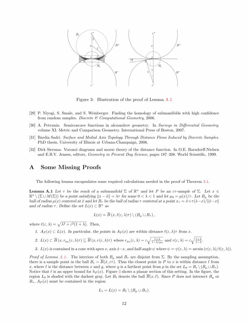
Figure 3: Illustration of the proof of Lemma A.1

[29] P. Niyogi, S. Smale, and S. Weinberger. Finding the homology of submanifolds with high confidencefrom random samples. Discrete & Computational Geometry, 2006.

[30] A. Petrunin. Semiconcave functions in alexandrov geometry. In Surveys in Differential Geometry,volume XI: Metric and Comparison Geometry. International Press of Boston, 2007.

[31] Bardia Sadri. Surface and Medial Axis Topology Through Distance Flows Induced by Discrete Samples.PhD thesis, University of Illinois at Urbana-Champaign, 2006.

[32] Dirk Siersma. Voronoi diagrams and morse theory of the distance function. In O.E. Barndorff-Nielsenand E.B.V. Jensen, editors, Geometry in Present Day Science, pages 187–208. World Scientific, 1999.

A Some Missing Proofs

The following lemma encapsulates some required calculations needed in the proof of Theorem 3.1.

Lemma A.1 Let τ be the reach of a submanifold Σ of Rn and let P be an ετ -sample of Σ. Let x ∈Rn \ (Σ∪M(Σ)) be a point satisfying ‖x− x‖ = λτ for some 0 < λ < 1 and let µ0 = µ(x)/τ . Let Bµ be theball of radius µ(x) centered at x and let Bτ be the ball of radius τ centered at a point xτ = x+τ(x−x)/‖x−x‖and of radius τ . Define the set L(x) ⊂ Rn as

L(x) = B (x, `(ε, λ)τ) \ (Bµ ∪Bτ ) ,

where `(ε, λ) =√λ2 + ε2(1 + λ). Then,

1. AP (x) ⊂ L(x). In particular, the points in AP (x) are within distance `(ε, λ)τ from x.

2. L(x) ⊂ B (x, rµ0(ε, λ)τ) ⊆ B (x, r(ε, λ)τ) where rµ0(ε, λ) = ε√

1+λ1−λ/µ0

and r(ε, λ) = ε√

1+λ1−λ .

3. L(x) is contained in a cone with apex x, axis x−x, and half-angle ψ where ψ = ψ(ε, λ) = arcsin (r(ε, λ)/`(ε, λ)).

Proof of Lemma A.1. The interiors of both Bµ and Bτ are disjoint from Σ. By the sampling assumption,there is a sample point in the ball Bε = B(x, ετ). Thus the closest point in P to x is within distance ` fromx, where ` is the distance between x and y, where y is a farthest point from p in the set L0 = Bε \ (Bµ∪Bτ ).Notice that ` is an upper bound for hP (x). Figure 3 shows a planar section of this setting. In the figure, theregion L0 is shaded with the darkest gray. Let B` denote the ball B(x, `). Since P does not intersect Bµ orBτ , AP (x) must be contained in the region

L1 = L(x) = B` \ (Bµ ∪Bτ ).

12

Let z be a point in this region farthest away from x and let r = ‖x− z‖. Let γ be the angle between y − xand the hyper-plane tangent to Σ at x and normal to x− x. It can be easily seen from Figure 3 (right) thatsin γ = ε/2.

To simplify notation, let us take τ as unit length. Since the angle ](y − x, x − x) is π/2 + γ we haveusing the cosine rule

`2 = ‖x− z‖2 = ‖x− y‖2

= λ2 + ε2 − 2ελ cos(π/2 + γ)

= λ2 + ε2 − 2ελ sin γ

= λ2 + ε2(1 + λ).

Now by applying the cosine rule to the triangle xzx, we have for the angle β = ](x− x, z − x)

cosβ =µ20 + (µ0 − λ)2 − `2

2µ0(µ0 − λ)

=µ20 + (µ0 − λ)2 − λ2 − ε2(1 + λ)

2µ0(µ0 − λ)

= 1− ε2

2µ20

· 1 + λ

1− λ/µ0.

If we rewrite the above equality as

cosβ = 1− 2

(ε

2µ0

√1 + λ

1− λ/µ0

)2

,

and observe on the figure that sin(β/2) = (r/2)/µ0, we can use the identity cosβ = 1−2 sin2(β/2) to obtain,

r = ε ·

√1 + λ

1− λ/µ0.

To complete the proof, we need to only show that the angle β′ = ](x − x, z − x) is smaller than ψ(ε, δ) asgiven in the statement of the Lemma. From the figure sinβ′ = h/` where h is the distance between z andthe line supporting the segment xx. Since h ≤ r, sinβ′ ≤ r/l = sinψ. �

Proof of Theorem 3.1. For simplicity we scale the distances so as to have τ = 1. Refer Figure 3 in theproof of Lemma A.1 (Appendix A). First observe that if c is at infinity, the open halfspace whose boundaryis tangent to Σ at c and contains c, is disjoint from Σ and therefore from P . This immediately implies thatc cannot be a critical point. Thus we assume that c is at finite distance from c.

By Lemma A.1, AP (x) ⊂ B` = B(x, `), where ` = `(ε, λ) as defined in Lemma A.1. On the otherhand AP (x) is disjoint from Bµ = B(x, µ) where µ = µ(x). Let H be the hyperplane normal to x − xthrough x and let R be the radius of the ball of intersection between H and Bµ. The plane H is at distance‖x− x‖ = µ(x)− λ from x. By the Pythagorean theorem

R2 = µ2 − (µ− λ)2.

If the radius ` of B` is less than R, then B` \Bµ is strictly contained in the open half-spaces of Rn \H thatcontains x. Since x ∈ H, this implies that x 6∈ conv(B` \ Bµ) which further entails that x 6∈ convAP (x).Since dP (x) ∈ convAP (x), this would imply that ](x−x, vP (x)) < π/2. In particular, x cannot be a criticalpoint if R > ` or equivalently if

µ2 − (µ− λ)2 > λ2 + ε2(1 + λ).

Rearranging the above inequality gives us

2λ2 + (ε2 − 2µ)λ+ ε2 < 0.

13

Solving for λ, we get λmin < λ < λmax, where λmin = 12

(µ− ε2/2−

√(µ− ε2/2)

2 − 2ε2)

and λmax =

12

(µ− ε2/2 +

√(µ− ε2/2)

2 − 2ε2)

. Since µ ≥ 1, ε ≤ 1/√

3 is sufficient to have (µ−ε2/2)2−2ε2 ≥ 0. Thus

for ε ≤ 1/√

3, both λmin and λmax are real. The assumption of ε ≤ 1/√

3 can be written as 3ε2 ≤ 1 fromwhich

2ε2 + 1 ≤ 2− ε2 ≤ 2µ− ε2 = 2(µ− ε2/2).

Multiplying by 2ε2 ≥ 0, gives us2ε2(2ε2 + 1) ≤ 4ε2(µ− ε2/2).

By adding (µ− ε2/2)2 to both sides and rearranging we get

(µ− ε2/2)2 − 2ε2 ≥((µ− ε2/2)− 2ε2

)2.

The smaller side being non-negative allows us to take square roots of both sides which by rearranging resultsλmin ≤ ε2. As for λmax, using the inequality

√1− t ≥ 1− t for 0 ≤ t ≤ 1

λmax =1

2(µ− ε2/2)

(1 +

√1− 2ε2

(µ− ε2/2)2

)

≥ 1

2(µ− ε2/2)

(2− 2ε2

(µ− ε2/2)2

)= µ− ε2/2− ε2

µ− ε2/2≥ µ− ε2/2− ε2

1− ε2/2≥ µ− 2ε2.

Thus if ε2 < λ < µ − 2ε2, the point x is separated from convAP (x) and therefore x cannot be a criticalpoint. To complete the proof, we note that µ ≥ τ = 1. �

Proof of Lemma 3.3. Consider the retraction map r : Σc → cl Σcδ given by

r(x) =

{x+ δτ · (x− x)/‖x− x‖ x ∈ Σc \ cl Σcδx x ∈ cl Σcδ

The map r is continuous on Σc \cl Σcδ since (x− x)/‖x− x‖ changes continuously with x (because the surfaceis smooth), the map x 7→ x is continuous because the only points of discontinuity of this map are medialaxis points of which there are none in Σc \ cl Σcδ. The continuity of r on all of its domain follows from agluing argument using the fact that the points on the boundary of Σcδ are mapped to themselves both withthe identity map and with the mapping x 7→ x+ δτ · (x− x)/‖x− x‖.

If we now define the map R : [0, 1]× Σc → cl Σcδ as

R(t, x) =

{(1− t)x+ tr(x) x ∈ Σc \ cl Σcδx x ∈ cl Σcδ,

the map R is a straight-line homotopy from the identity of Σc to the retraction map r. �

B Proof of Lemma 3.4

Lemma B.1 Let x be a point satisfying ‖x− x‖ = δτ . Then, the angle α that vP (x) makes with x− x isbounded by

arccos

(2δ(1− ε− δ)− ε2

2(1− δ)(δ + ε)

),

provided that the argument of the arccos is between 0 and 1.

Proof. Let c be the point on the line segment xx at distance τ from x.

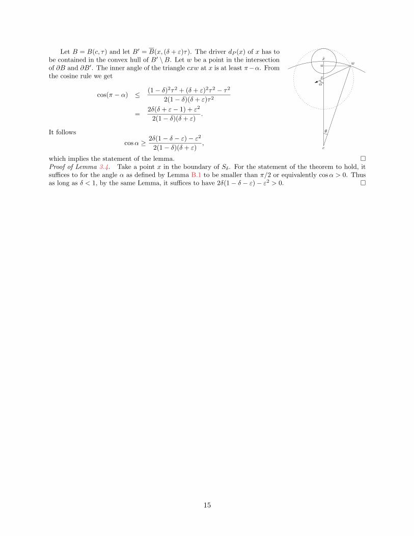
14

x

α

x

u

θ

c

w

Let B = B(c, τ) and let B′ = B(x, (δ + ε)τ). The driver dP (x) of x has tobe contained in the convex hull of B′ \B. Let w be a point in the intersectionof ∂B and ∂B′. The inner angle of the triangle cxw at x is at least π−α. Fromthe cosine rule we get

cos(π − α) ≤ (1− δ)2τ2 + (δ + ε)2τ2 − τ2

2(1− δ)(δ + ε)τ2

=2δ(δ + ε− 1) + ε2

2(1− δ)(δ + ε).

It follows

cosα ≥ 2δ(1− δ − ε)− ε2

2(1− δ)(δ + ε),

which implies the statement of the lemma. �Proof of Lemma 3.4. Take a point x in the boundary of Sδ. For the statement of the theorem to hold, itsuffices to for the angle α as defined by Lemma B.1 to be smaller than π/2 or equivalently cosα > 0. Thusas long as δ < 1, by the same Lemma, it suffices to have 2δ(1− δ − ε)− ε2 > 0. �

15