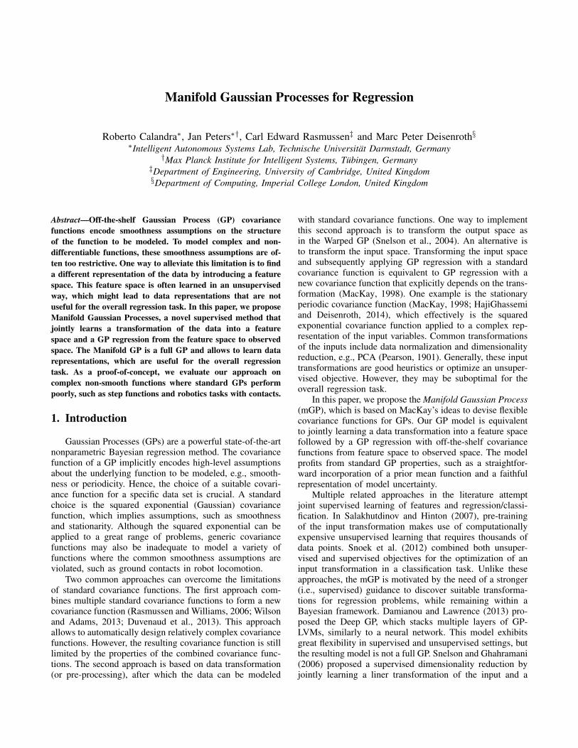
Manifold Gaussian Processes for Regression

Roberto Calandra∗, Jan Peters∗†, Carl Edward Rasmussen‡ and Marc Peter Deisenroth§∗Intelligent Autonomous Systems Lab, Technische Universitat Darmstadt, Germany

†Max Planck Institute for Intelligent Systems, Tubingen, Germany‡Department of Engineering, University of Cambridge, United Kingdom§Department of Computing, Imperial College London, United Kingdom

Abstract—Off-the-shelf Gaussian Process (GP) covariancefunctions encode smoothness assumptions on the structureof the function to be modeled. To model complex and non-differentiable functions, these smoothness assumptions are of-ten too restrictive. One way to alleviate this limitation is to finda different representation of the data by introducing a featurespace. This feature space is often learned in an unsupervisedway, which might lead to data representations that are notuseful for the overall regression task. In this paper, we proposeManifold Gaussian Processes, a novel supervised method thatjointly learns a transformation of the data into a featurespace and a GP regression from the feature space to observedspace. The Manifold GP is a full GP and allows to learn datarepresentations, which are useful for the overall regressiontask. As a proof-of-concept, we evaluate our approach oncomplex non-smooth functions where standard GPs performpoorly, such as step functions and robotics tasks with contacts.

1. Introduction

Gaussian Processes (GPs) are a powerful state-of-the-artnonparametric Bayesian regression method. The covariancefunction of a GP implicitly encodes high-level assumptionsabout the underlying function to be modeled, e.g., smooth-ness or periodicity. Hence, the choice of a suitable covari-ance function for a specific data set is crucial. A standardchoice is the squared exponential (Gaussian) covariancefunction, which implies assumptions, such as smoothnessand stationarity. Although the squared exponential can beapplied to a great range of problems, generic covariancefunctions may also be inadequate to model a variety offunctions where the common smoothness assumptions areviolated, such as ground contacts in robot locomotion.

Two common approaches can overcome the limitationsof standard covariance functions. The first approach com-bines multiple standard covariance functions to form a newcovariance function (Rasmussen and Williams, 2006; Wilsonand Adams, 2013; Duvenaud et al., 2013). This approachallows to automatically design relatively complex covariancefunctions. However, the resulting covariance function is stilllimited by the properties of the combined covariance func-tions. The second approach is based on data transformation(or pre-processing), after which the data can be modeled

with standard covariance functions. One way to implementthis second approach is to transform the output space asin the Warped GP (Snelson et al., 2004). An alternative isto transform the input space. Transforming the input spaceand subsequently applying GP regression with a standardcovariance function is equivalent to GP regression with anew covariance function that explicitly depends on the trans-formation (MacKay, 1998). One example is the stationaryperiodic covariance function (MacKay, 1998; HajiGhassemiand Deisenroth, 2014), which effectively is the squaredexponential covariance function applied to a complex rep-resentation of the input variables. Common transformationsof the inputs include data normalization and dimensionalityreduction, e.g., PCA (Pearson, 1901). Generally, these inputtransformations are good heuristics or optimize an unsuper-vised objective. However, they may be suboptimal for theoverall regression task.

In this paper, we propose the Manifold Gaussian Process(mGP), which is based on MacKay’s ideas to devise flexiblecovariance functions for GPs. Our GP model is equivalentto jointly learning a data transformation into a feature spacefollowed by a GP regression with off-the-shelf covariancefunctions from feature space to observed space. The modelprofits from standard GP properties, such as a straightfor-ward incorporation of a prior mean function and a faithfulrepresentation of model uncertainty.

Multiple related approaches in the literature attemptjoint supervised learning of features and regression/classi-fication. In Salakhutdinov and Hinton (2007), pre-trainingof the input transformation makes use of computationallyexpensive unsupervised learning that requires thousands ofdata points. Snoek et al. (2012) combined both unsuper-vised and supervised objectives for the optimization of aninput transformation in a classification task. Unlike theseapproaches, the mGP is motivated by the need of a stronger(i.e., supervised) guidance to discover suitable transforma-tions for regression problems, while remaining within aBayesian framework. Damianou and Lawrence (2013) pro-posed the Deep GP, which stacks multiple layers of GP-LVMs, similarly to a neural network. This model exhibitsgreat flexibility in supervised and unsupervised settings, butthe resulting model is not a full GP. Snelson and Ghahramani(2006) proposed a supervised dimensionality reduction byjointly learning a liner transformation of the input and a

X Y

Regression

F

(a) Supervised learning of a regression function.

X YL

Regression

M G

(b) Supervised learning integrating out a latent space isintractable.

X YH

Input Transformation

Regression

M G|M

(c) Unsupervisedly learned input transformation M fol-lowed by a conditional regression G|M .

X YH

Input Transformation + Regression

M G

(d) Manifold GP: joint supervised learning of the inputtransformation M and the regression task G.

Figure 1: Different regression settings to learn the function F : X → Y . (a) Standard supervised regression. (b) Regressionwith an auxiliary latent space L that allows to simplify the task. In a full Bayesian framework, L would be integrated out,which is analytically intractable. (c) Decomposition of the overall regression task F into discovering a feature space Husing the map M and a subsequent (conditional) regression G|M . (d) Our mGP learns the mappings G and M jointly.

GP. Snoek et al. (2014) transformed the input data usinga Beta distribution whose parameters were learned jointlywith the GP. However, the purpose of this transformation isto account for skewness in the data, while mGP allows fora more general class of transformations.

2. Manifold Gaussian Processes

In the following, we review methods for regression,which may use latent or feature spaces. Then, we providea brief introduction to Gaussian Process regression. Finally,we introduce the Manifold Gaussian Processes, our novelapproach to jointly learning a regression model and a suit-able feature representation of the data.

2.1. Regression with Learned Features

We assume N training inputs xn ∈ X ⊆ RD andrespective outputs yn ∈ Y ⊆ R, where yn = F (xn) + w,w ∼ N

(0, σ2

w

), n = 1, . . . , N . The training data is denoted

byX and Y for the inputs and targets, respectively. We con-sider the task of learning a regression function F : X → Y .The corresponding setting is given in Figure 1a. Discoveringthe regression function F is often challenging for nonlinearfunctions. A typical way to simplify and distribute the com-plexity of the regression problem is to introduce an auxiliarylatent space L. The function F can then be decomposedinto F = G ◦M , where M : X → L and G : L → Y ,as shown in Figure 1b. In a full Bayesian framework, thelatent space L is integrated out to solve the regression

task F , which is often analytically unfeasible (Schmidt andO’Hagan, 2003).

A common approximation to the full Bayesian frame-work is to introduce a deterministic feature space H, and tofind the mappings M and G in two consecutive steps. First,M is determined by means of unsupervised feature learning.Second, the regression G is learned supervisedly as a con-ditional model G|M , see Figure 1c. The use of this featurespace can reduce the complexity of the learning problem.For example, for complicated non-linear functions a higher-dimensional (overcomplete) representation H allows learn-ing a simpler mapping G : H → Y . For high-dimensionalinputs, the data often lies on a lower-dimensional mani-fold H, e.g., due to non-discriminant or strongly correlatedcovariates. The lower-dimensional feature space H reducesthe effect of the curse of dimensionality. In this paper, wefocus on modeling complex functions with a relatively low-dimensional input space, which, nonetheless, cannot be wellmodeled by off-the-shelf GP covariance functions.

Typically, unsupervised feature learning methods de-termine the mapping M by optimizing an unsupervisedobjective, independent from the objective of the overallregression F . Examples of such unsupervised objectives arethe minimization of the input reconstruction error (auto-encoders (Vincent et al., 2008)), maximization of the vari-ance (PCA (Pearson, 1901)), maximization of the statisticalindependence (ICA (Hyvarinen and Oja, 2000)), or thepreservation of the distances between data (isomap (Tenen-baum et al., 2000) or LLE (Roweis and Saul, 2000)). Inthe context of regression, an unsupervised approach for

feature learning can be insufficient as the learned datarepresentation H might not suit the overall regressiontask F (Wahlstrom et al., 2015): Unsupervised and super-vised learning optimize different objectives, which do notnecessarily match, e.g., minimizing the reconstruction erroras unsupervised objective and maximizing the marginal like-lihood as supervised objective. An approach where featurelearning is performed in a supervised manner can insteadguide learning the feature mapping M toward representa-tions that are useful for the overall regression F = G ◦M .This intuition is the key insight of our Manifold GaussianProcesses, where the feature mapping M and the GP Gare learned jointly using the same supervised objective asdepicted in Figure 1d.

2.2. Gaussian Process Regression

GPs are a state-of-the-art probabilistic non-parametricregression method (Rasmussen and Williams, 2006). Sucha GP is a distribution over functions

F ∼ GP (m, k) (1)

and fully defined by a mean function m (in our case m ≡ 0)and a covariance function k. The GP predictive distributionat a test input x∗ is given by

p (F(x∗)|D,x∗) = N(µ(x∗), σ

2(x∗)), (2)

µ(x∗) = kT∗ (K + σ2

wI)−1Y , (3)

σ2(x∗) = k∗∗ − kT∗ (K + σ2wI)

−1k∗ , (4)

where D = {X,Y } is the training data, K is the ker-nel matrix with Kij = k(xi,xj), k∗∗ = k(x∗,x∗),k∗ = k(X,x∗) and σ2

w is the measurement noise variance.In our experiments, we use different covariance functionsk. Specifically, we use the squared exponential covariancefunction with Automatic Relevance Determination (ARD)

kSE(xp,xq) = σ2f exp

(− 1

2 (xp−xq)TΛ−1(xp−xq)

), (5)

with Λ = diag([l21, ..., l2D]), where li are the characteristic

length-scales, and σ2f is the variance of the latent function F .

Furthermore, we use the neural network covariance function

kNN(xp,xq) = σ2f sin

−1

(xT

p Pxq√(1+xT

p Pxp)(1+xTq Pxq)

), (6)

where P is a weight matrix. Each covariance functionpossesses various hyperparameters θ to be selected. Thisselection is performed by minimizing the Negative LogMarginal Likelihood (NLML)

NLML(θ) = − log p(Y |X,θ) (7)·= 1

2YT (Kθ + σ2

wI)−1Y + 1

2 log |Kθ + σ2wI|

Using the chain-rule, the corresponding gradient can becomputed analytically as

∂NLML(θ)∂θ

=∂NLML(θ)

∂Kθ

∂Kθ

∂θ, (8)

which allows us to optimize the hyperparameters usingQuasi-Newton optimization, e.g., L-BFGS (Liu and No-cedal, 1989).

2.3. Manifold Gaussian Processes

In this section, we describe the mGP model and itsparameters θmGP itself, and relate it to standard GP regres-sion. Furthermore, we detail training and prediction with themGP.

2.3.1. Model. As shown in Figure 1d, the mGP considersthe overall regression as a composition of functions

F = G ◦M . (9)

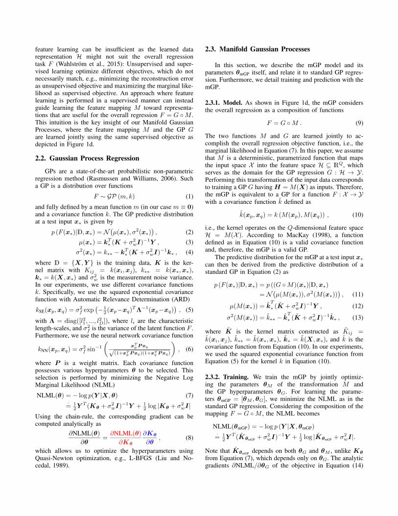
The two functions M and G are learned jointly to ac-complish the overall regression objective function, i.e., themarginal likelihood in Equation (7). In this paper, we assumethat M is a deterministic, parametrized function that mapsthe input space X into the feature space H ⊆ RQ, whichserves as the domain for the GP regression G : H → Y .Performing this transformation of the input data correspondsto training a GP G havingH =M(X) as inputs. Therefore,the mGP is equivalent to a GP for a function F : X → Ywith a covariance function k defined as

k(xp,xq) = k (M(xp),M(xq)) , (10)

i.e., the kernel operates on the Q-dimensional feature spaceH = M(X ). According to MacKay (1998), a functiondefined as in Equation (10) is a valid covariance functionand, therefore, the mGP is a valid GP.

The predictive distribution for the mGP at a test input x∗can then be derived from the predictive distribution of astandard GP in Equation (2) as

p (F(x∗)|D,x∗) = p ((G ◦M)(x∗)|D,x∗)

= N(µ(M(x∗)), σ

2(M(x∗))), (11)

µ(M(x∗)) = kT

∗ (K + σ2wI)

−1Y , (12)

σ2(M(x∗)) = k∗∗ − kT

∗ (K + σ2wI)

−1k∗ , (13)

where K is the kernel matrix constructed as Kij =k(xi,xj), k∗∗ = k(x∗,x∗), k∗ = k(X,x∗), and k is thecovariance function from Equation (10). In our experiments,we used the squared exponential covariance function fromEquation (5) for the kernel k in Equation (10).

2.3.2. Training. We train the mGP by jointly optimiz-ing the parameters θM of the transformation M andthe GP hyperparameters θG. For learning the parame-ters θmGP = [θM ,θG], we minimize the NLML as in thestandard GP regression. Considering the composition of themapping F = G ◦M , the NLML becomes

NLML(θmGP) = − log p (Y |X,θmGP)·= 1

2YT (KθmGP + σ2

wI)−1Y + 1

2 log |KθmGP + σ2wI|.

Note that KθmGP depends on both θG and θM , unlike Kθ

from Equation (7), which depends only on θG. The analyticgradients ∂NLML/∂θG of the objective in Equation (14)

with respect to the parameters θG are computed as in thestandard GP, i.e.,

∂NLML(θmGP)

∂θG=∂NLML(θmGP)

∂KθmGP

∂KθmGP

∂θG. (14)

The gradients of the parameters θM of the feature mappingare computed by applying the chain-rule

∂NLML(θmGP)

∂θM=∂NLML(θmGP)

∂KθmGP

∂KθmGP

∂H

∂H

∂θM, (15)

where only ∂H/∂θM depends on the chosen input trans-formation M , while ∂KθmGP/∂H is the gradient of thekernel matrix with respect to the Q-dimensional GP traininginputs H = M(X). Similarly to standard GP, the param-eters θmGP in the mGP can be obtained using off-the-shelfoptimization methods.

2.3.3. Input Transformation. Our approach can use anydeterministic parametric data transformation M . We focuson multi-layer neural networks and define their structure as[q1− . . .− ql] where l is the number of layers, and qi is thenumber of neurons of the ith layer. Each layer i = 1, . . . , lof the neural network performs the transformation

Ti(Z) = σ (W iZ +Bi) , (16)

where Z is the input of the layer, σ is the transfer func-tion, and W i and Bi are the weights and the bias ofthe layer, respectively. Therefore, the input transforma-tion M of Equation (9) is M(X) = (Tl ◦ . . . ◦T1)(X).The parameters θM of the neural network M arethe weights and biases of the whole network, so thatθM = [W 1,B1, . . . ,W l,Bl]. The gradients ∂H/∂θM inEquation (15) are computed by repeated application of thechain-rule (backpropagation).

3. Experimental Results

To demonstrate the efficiency of our proposed approach,we apply the mGP to challenging benchmark problemsand a real-world regression task. First, we demonstrate thatmGPs can be successfully applied to learning discontin-uous functions, a daunting undertaking with an off-the-shelf covariance function, due to its underlying smoothnessassumptions. Second, we evaluate mGPs on a function withmultiple natural length-scales. Third, we assess mGPs onreal data from a walking bipedal robot. The locomotiondata set is highly challenging due to ground contacts, whichcause the regression function to violate standard smoothnessassumptions.

To evaluate the goodness of the different models on thetraining set, we consider the NLML previously introducedin Equation (7) and (14). Additionally, for the test set, wemake use of the Negative Log Predictive Probability (NLPP)

− log p(y = y∗|X,x∗,Y ,θ) , (17)

where the y∗ is the test target for the input x∗ as computedfor the standard GP in Equation (2) and (11) for the mGPmodel.

We compare our mGP approach with GPs using the SE-ARD and NN covariance functions, which implement themodel in Figure 1a. Moreover, we evaluate two unsupervisedfeature extraction methods, Random Embeddings and PCA,followed by a GP SE-ARD, which implements the modelin Figure 1c.1 For the model in Figure 1d, we consider twovariants of mGP with the log-sigmoid σ (x) = 1/(1 + e−x)and the identity σ (x) = x transfer functions. These twotransfer functions lead to a non-linear and a linear trans-formation M , respectively.

3.1. Step Function

In the following, we consider the step function

y = F(x) + w , w ∼ N(0, 0.012

),

F(x) =

{0 if x ≤ 0

1 if x > 0. (18)

For training, 100 inputs points are sampled from N(0, 1)

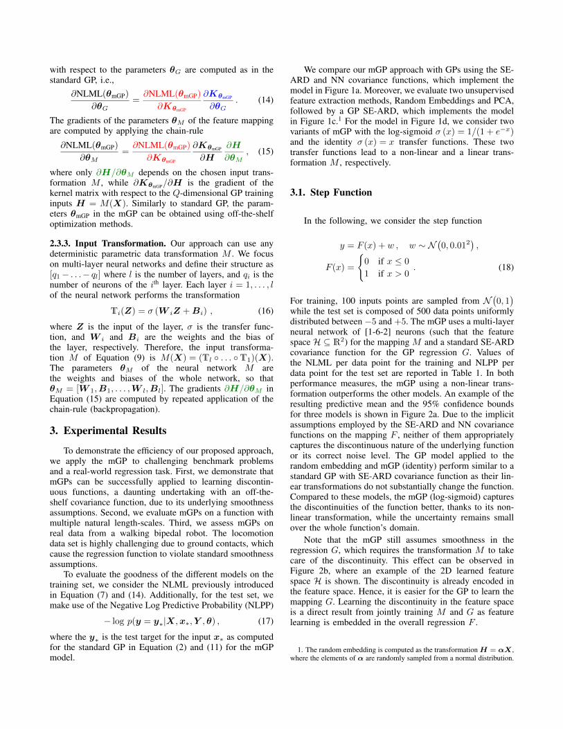
while the test set is composed of 500 data points uniformlydistributed between −5 and +5. The mGP uses a multi-layerneural network of [1-6-2] neurons (such that the featurespace H ⊆ R2) for the mapping M and a standard SE-ARDcovariance function for the GP regression G. Values ofthe NLML per data point for the training and NLPP perdata point for the test set are reported in Table 1. In bothperformance measures, the mGP using a non-linear trans-formation outperforms the other models. An example of theresulting predictive mean and the 95% confidence boundsfor three models is shown in Figure 2a. Due to the implicitassumptions employed by the SE-ARD and NN covariancefunctions on the mapping F , neither of them appropriatelycaptures the discontinuous nature of the underlying functionor its correct noise level. The GP model applied to therandom embedding and mGP (identity) perform similar to astandard GP with SE-ARD covariance function as their lin-ear transformations do not substantially change the function.Compared to these models, the mGP (log-sigmoid) capturesthe discontinuities of the function better, thanks to its non-linear transformation, while the uncertainty remains smallover the whole function’s domain.

Note that the mGP still assumes smoothness in theregression G, which requires the transformation M to takecare of the discontinuity. This effect can be observed inFigure 2b, where an example of the 2D learned featurespace H is shown. The discontinuity is already encoded inthe feature space. Hence, it is easier for the GP to learn themapping G. Learning the discontinuity in the feature spaceis a direct result from jointly training M and G as featurelearning is embedded in the overall regression F .

1. The random embedding is computed as the transformationH = αX ,where the elements of α are randomly sampled from a normal distribution.

-5 -4 -3 -2 -1 0 1 2 3 4 5-0.5

0

0.5

1

1.5GP SE-ARD

Input X

Outp

ut

Y

GP NN

mGP

Training set

(a) GP prediction.

-5 -4 -3 -2 -1 0 1 2 3 4 5-0.2

0

0.2

0.4

0.6

0.8

1

Latent dimension 1

Latent dimension 2

Input X

Featu

re s

pace

H

(b) Learned mapping M using mGP (log-sigmoid).

Figure 2: Step Function: (a) Predictive mean and 95% confidence bounds for a GP with SE-ARD covariance function(blue solid), a GP with NN covariance function (red dotted) and a log-sigmoid mGP (green dashed) on the step functionof Equation (18). The discontinuity is captured better by an mGP than by a regular GP with either SE-ARD or NNcovariance functions. (b) The 2D feature space H discovered by the non-linear mapping M as a function of the input X .The discontinuity of the modeled function is already captured by the non-linear mapping M . Hence, the mapping fromfeature space H to the output Y is smooth and can be easily managed by the GP.

Table 1: Step Function: Negative Log Marginal Likelihood(NLML) and Negative Log Predictive Probability (NLPP)per data point for the step function of Equation (18). ThemGP (log-sigmoid) captures the nature of the underlyingfunction better than a standard GP in both the training andtest sets.

Method Training set Test setNLML RMSE NLPP RMSE

GP SE-ARD −0.68 1.00× 10−2 +0.50× 10−3 0.58GP NN −1.49 0.57× 10−2 +0.02× 10−3 0.14mGP (log-sigmoid) −2.84 1.06× 10−2 −6.34× 10−3 0.02mGP (identity) −0.68 1.00× 10−2 +0.50× 10−3 0.58RandEmb + GP SE-ARD −0.77 5.26× 10−2 +0.51× 10−3 0.52

3.2. Multiple Length-Scales

In the following, we demonstrate that the mGP canbe used to model functions that possess multiple intrinsiclength-scales. For this purpose, we rotate the function

y = 1−N(x2|3, 0.52

)−N

(x2| − 3, 0.52

)+ x1

100 (19)

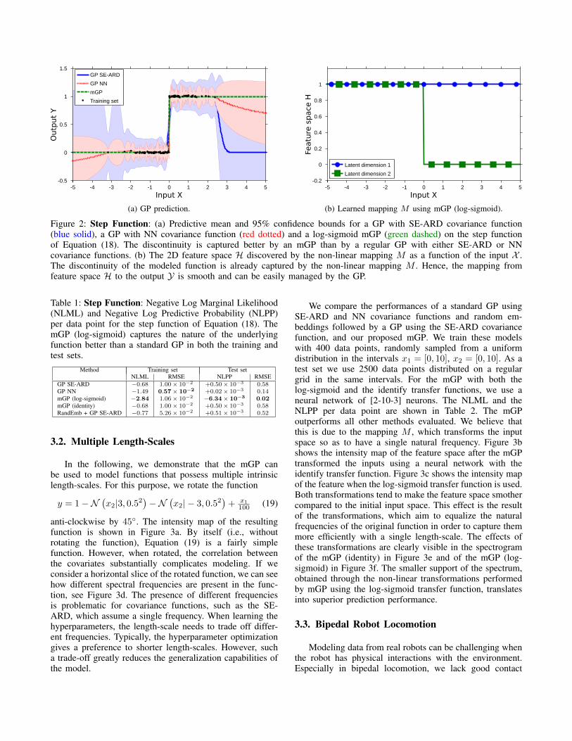
anti-clockwise by 45◦. The intensity map of the resultingfunction is shown in Figure 3a. By itself (i.e., withoutrotating the function), Equation (19) is a fairly simplefunction. However, when rotated, the correlation betweenthe covariates substantially complicates modeling. If weconsider a horizontal slice of the rotated function, we can seehow different spectral frequencies are present in the func-tion, see Figure 3d. The presence of different frequenciesis problematic for covariance functions, such as the SE-ARD, which assume a single frequency. When learning thehyperparameters, the length-scale needs to trade off differ-ent frequencies. Typically, the hyperparameter optimizationgives a preference to shorter length-scales. However, sucha trade-off greatly reduces the generalization capabilities ofthe model.

We compare the performances of a standard GP usingSE-ARD and NN covariance functions and random em-beddings followed by a GP using the SE-ARD covariancefunction, and our proposed mGP. We train these modelswith 400 data points, randomly sampled from a uniformdistribution in the intervals x1 = [0, 10], x2 = [0, 10]. As atest set we use 2500 data points distributed on a regulargrid in the same intervals. For the mGP with both thelog-sigmoid and the identify transfer functions, we use aneural network of [2-10-3] neurons. The NLML and theNLPP per data point are shown in Table 2. The mGPoutperforms all other methods evaluated. We believe thatthis is due to the mapping M , which transforms the inputspace so as to have a single natural frequency. Figure 3bshows the intensity map of the feature space after the mGPtransformed the inputs using a neural network with theidentify transfer function. Figure 3c shows the intensity mapof the feature when the log-sigmoid transfer function is used.Both transformations tend to make the feature space smothercompared to the initial input space. This effect is the resultof the transformations, which aim to equalize the naturalfrequencies of the original function in order to capture themmore efficiently with a single length-scale. The effects ofthese transformations are clearly visible in the spectrogramof the mGP (identity) in Figure 3e and of the mGP (log-sigmoid) in Figure 3f. The smaller support of the spectrum,obtained through the non-linear transformations performedby mGP using the log-sigmoid transfer function, translatesinto superior prediction performance.

3.3. Bipedal Robot Locomotion

Modeling data from real robots can be challenging whenthe robot has physical interactions with the environment.Especially in bipedal locomotion, we lack good contact

x 2

x1

(a) Intensity map of the function.

h1

h 2

(b) Intensity map of the learned featurespace for the mGP (identity).

h1

h 2

(c) Intensity map of the learned featurespace for the mGP (log-sigmoid).

Magnitude

Frequency

(d) Spectrum of the function.

Magnitude

Frequency

(e) Spectrum of the learned feature spacefor the mGP (identity).

Magnitude

Frequency

(f) Spectrum of the learned feature spacefor the mGP (log-sigmoid).

Figure 3: Multiple Length-Scales: Intensity map of (a) the considered function, (b) the learned feature space of the mGPwith a linear activation function and (c) with a log-sigmoid activation. (d)–(f) The corresponding Spectrum for (d) theoriginal function and the learned feature space for (e) mGP (identity) and (f) mGP (log-sigmoid). The spectral analysisof the original function shows the presence of multiple frequencies. The transformations learned by both variants of mGPfocus the spectrum of the feature space towards a more compact frequencies support.

Table 2: Multiple Length-Scales: NLML per data point forthe training set and NLPP per data point for the test set. ThemGP captures the nature of the underlying function betterthan a standard GP in both the training and test sets.

Method Training set Test setNLML RMSE NLPP RMSE

GP SE-ARD −2.46 0.40× 10−3 −4.34 1.51× 10−2

GP NN −1.57 1.52× 10−3 −2.53 6.32× 10−2

mGP (log-sigmoid) −6.61 0.37× 10−4 −7.37 0.58× 10−4

mGP (identity) −5.60 0.79× 10−4 −6.63 2.36× 10−3

RandEmb + GP SE-ARD −0.47 6.84× 10−3 −1.29 1.19× 10−1

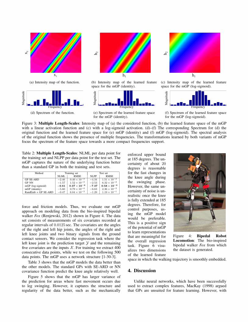
force and friction models. Thus, we evaluate our mGPapproach on modeling data from the bio-inspired bipedalwalker Fox (Renjewski, 2012) shown in Figure 4. The dataset consists of measurements of six covariates recorded atregular intervals of 0.0125 sec. The covariates are the anglesof the right and left hip joints, the angles of the right andleft knee joints and two binary signals from the groundcontact sensors. We consider the regression task where theleft knee joint is the prediction target Y and the remainingfive covariates are the inputs X . For training we extract 400consecutive data points, while we test on the following 500data points. The mGP uses a network structure [1-30-3].

Table 3 shows that the mGP models the data better thanthe other models. The standard GPs with SE-ARD or NNcovariance function predict the knee angle relatively well.

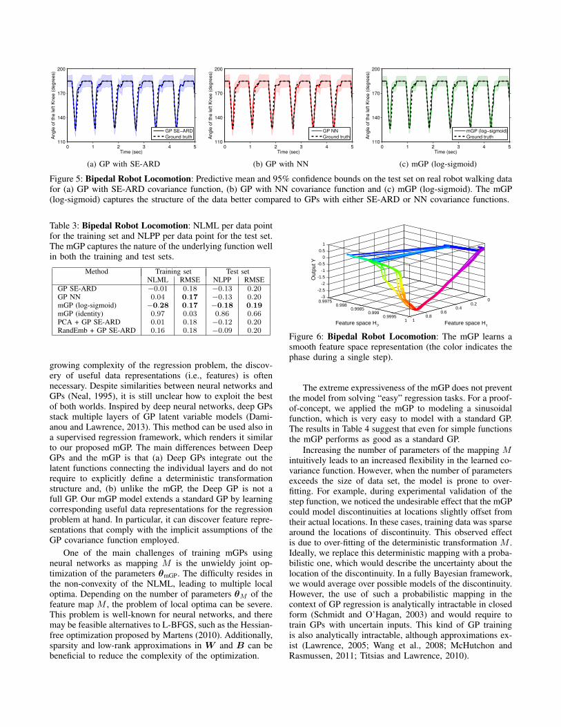
Figure 5 shows that the mGP has larger variance ofthe prediction for areas where fast movement occurs dueto leg swinging. However, it captures the structure andregularity of the data better, such as the mechanically

Figure 4: Bipedal RobotLocomotion: The bio-inspiredbipedal walker Fox from whichthe dataset is generated.

enforced upper boundat 185 degrees. The un-certainty of about 20degrees is reasonablefor the fast changes inthe knee angle duringthe swinging phase.However, the same un-certainty of noise is un-realistic once the kneeis fully extended at 185degrees. Therefore, forcontrol purposes, us-ing the mGP modelwould be preferable.This is a positive signof the potential of mGPto learn representationsthat are meaningful forthe overall regressiontask. Figure 6 visu-alizes two dimensionsof the learned featurespace in which the walking trajectory is smoothly embedded.

4. Discussion

Unlike neural networks, which have been successfullyused to extract complex features, MacKay (1998) arguedthat GPs are unsuited for feature learning. However, with

0 1 2 3 4 5110

140

170

200

Time (sec)

AngleoftheleftKnee(degrees)

GP SE−ARDGround truth

(a) GP with SE-ARD

0 1 2 3 4 5110

140

170

200

Time (sec)

Ang

leof

the

left

Kne

e(d

egre

es)

GP NNGround truth

(b) GP with NN

0 1 2 3 4 5110

140

170

200

Time (sec)

Ang

leof

the

left

Kne

e(d

egre

es)

mGP (log−sigmoid)Ground truth

(c) mGP (log-sigmoid)

Figure 5: Bipedal Robot Locomotion: Predictive mean and 95% confidence bounds on the test set on real robot walking datafor (a) GP with SE-ARD covariance function, (b) GP with NN covariance function and (c) mGP (log-sigmoid). The mGP(log-sigmoid) captures the structure of the data better compared to GPs with either SE-ARD or NN covariance functions.

Table 3: Bipedal Robot Locomotion: NLML per data pointfor the training set and NLPP per data point for the test set.The mGP captures the nature of the underlying function wellin both the training and test sets.

Method Training set Test setNLML RMSE NLPP RMSE

GP SE-ARD −0.01 0.18 −0.13 0.20GP NN 0.04 0.17 −0.13 0.20mGP (log-sigmoid) −0.28 0.17 −0.18 0.19mGP (identity) 0.97 0.03 0.86 0.66PCA + GP SE-ARD 0.01 0.18 −0.12 0.20RandEmb + GP SE-ARD 0.16 0.18 −0.09 0.20

growing complexity of the regression problem, the discov-ery of useful data representations (i.e., features) is oftennecessary. Despite similarities between neural networks andGPs (Neal, 1995), it is still unclear how to exploit the bestof both worlds. Inspired by deep neural networks, deep GPsstack multiple layers of GP latent variable models (Dami-anou and Lawrence, 2013). This method can be used also ina supervised regression framework, which renders it similarto our proposed mGP. The main differences between DeepGPs and the mGP is that (a) Deep GPs integrate out thelatent functions connecting the individual layers and do notrequire to explicitly define a deterministic transformationstructure and, (b) unlike the mGP, the Deep GP is not afull GP. Our mGP model extends a standard GP by learningcorresponding useful data representations for the regressionproblem at hand. In particular, it can discover feature repre-sentations that comply with the implicit assumptions of theGP covariance function employed.

One of the main challenges of training mGPs usingneural networks as mapping M is the unwieldy joint op-timization of the parameters θmGP. The difficulty resides inthe non-convexity of the NLML, leading to multiple localoptima. Depending on the number of parameters θM of thefeature map M , the problem of local optima can be severe.This problem is well-known for neural networks, and theremay be feasible alternatives to L-BFGS, such as the Hessian-free optimization proposed by Martens (2010). Additionally,sparsity and low-rank approximations in W and B can bebeneficial to reduce the complexity of the optimization.

Feature space H1

Feature space H2

Out

put Y

00.2

0.40.6

0.81

0.99750.998

0.99850.999

0.99951

-3

-2.5

-2

-1.5

-1

-0.5

0

0.5

1

Figure 6: Bipedal Robot Locomotion: The mGP learns asmooth feature space representation (the color indicates thephase during a single step).

The extreme expressiveness of the mGP does not preventthe model from solving “easy” regression tasks. For a proof-of-concept, we applied the mGP to modeling a sinusoidalfunction, which is very easy to model with a standard GP.The results in Table 4 suggest that even for simple functionsthe mGP performs as good as a standard GP.

Increasing the number of parameters of the mapping Mintuitively leads to an increased flexibility in the learned co-variance function. However, when the number of parametersexceeds the size of data set, the model is prone to over-fitting. For example, during experimental validation of thestep function, we noticed the undesirable effect that the mGPcould model discontinuities at locations slightly offset fromtheir actual locations. In these cases, training data was sparsearound the locations of discontinuity. This observed effectis due to over-fitting of the deterministic transformation M .Ideally, we replace this deterministic mapping with a proba-bilistic one, which would describe the uncertainty about thelocation of the discontinuity. In a fully Bayesian framework,we would average over possible models of the discontinuity.However, the use of such a probabilistic mapping in thecontext of GP regression is analytically intractable in closedform (Schmidt and O’Hagan, 2003) and would require totrain GPs with uncertain inputs. This kind of GP trainingis also analytically intractable, although approximations ex-ist (Lawrence, 2005; Wang et al., 2008; McHutchon andRasmussen, 2011; Titsias and Lawrence, 2010).

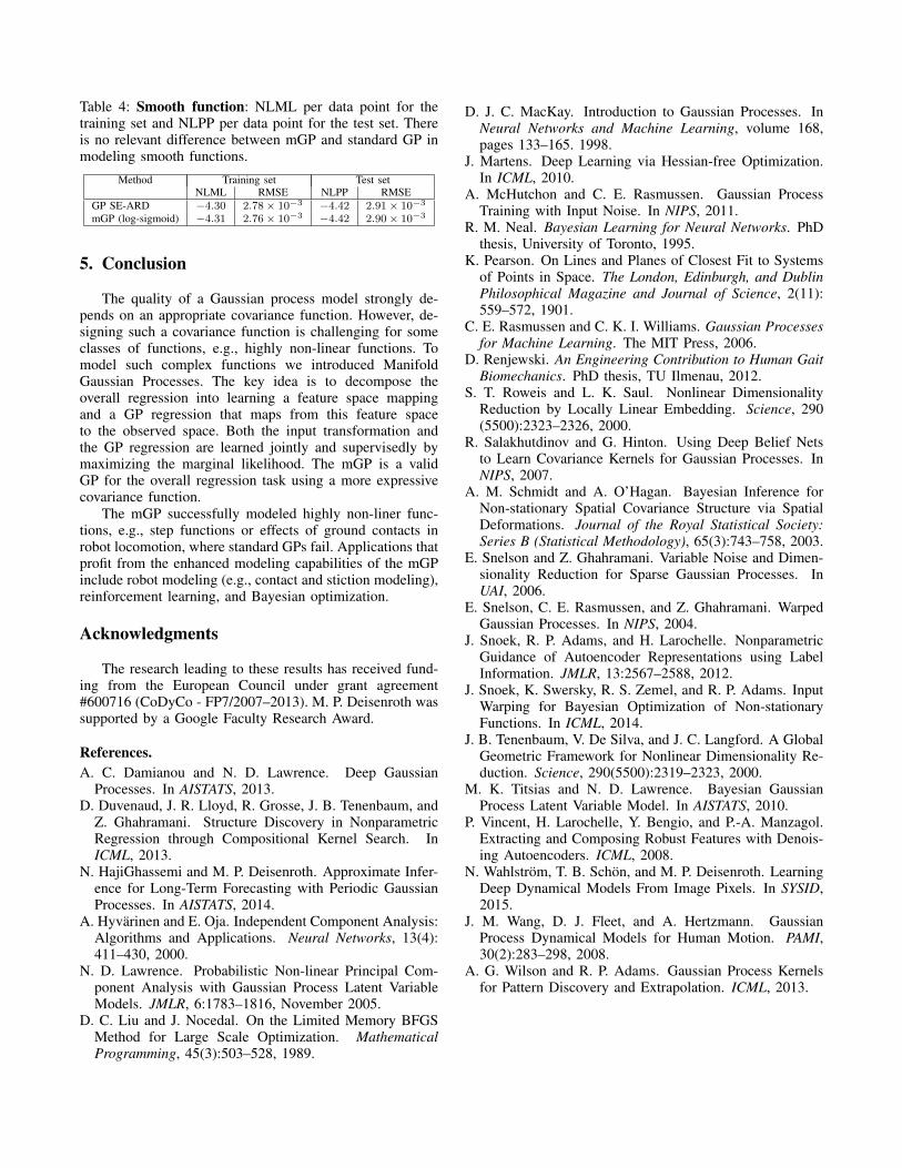
Table 4: Smooth function: NLML per data point for thetraining set and NLPP per data point for the test set. Thereis no relevant difference between mGP and standard GP inmodeling smooth functions.

Method Training set Test setNLML RMSE NLPP RMSE

GP SE-ARD −4.30 2.78× 10−3 −4.42 2.91× 10−3

mGP (log-sigmoid) −4.31 2.76× 10−3 −4.42 2.90× 10−3

5. Conclusion

The quality of a Gaussian process model strongly de-pends on an appropriate covariance function. However, de-signing such a covariance function is challenging for someclasses of functions, e.g., highly non-linear functions. Tomodel such complex functions we introduced ManifoldGaussian Processes. The key idea is to decompose theoverall regression into learning a feature space mappingand a GP regression that maps from this feature spaceto the observed space. Both the input transformation andthe GP regression are learned jointly and supervisedly bymaximizing the marginal likelihood. The mGP is a validGP for the overall regression task using a more expressivecovariance function.

The mGP successfully modeled highly non-liner func-tions, e.g., step functions or effects of ground contacts inrobot locomotion, where standard GPs fail. Applications thatprofit from the enhanced modeling capabilities of the mGPinclude robot modeling (e.g., contact and stiction modeling),reinforcement learning, and Bayesian optimization.

Acknowledgments

The research leading to these results has received fund-ing from the European Council under grant agreement#600716 (CoDyCo - FP7/2007–2013). M. P. Deisenroth wassupported by a Google Faculty Research Award.

References.A. C. Damianou and N. D. Lawrence. Deep Gaussian

Processes. In AISTATS, 2013.D. Duvenaud, J. R. Lloyd, R. Grosse, J. B. Tenenbaum, and

Z. Ghahramani. Structure Discovery in NonparametricRegression through Compositional Kernel Search. InICML, 2013.

N. HajiGhassemi and M. P. Deisenroth. Approximate Infer-ence for Long-Term Forecasting with Periodic GaussianProcesses. In AISTATS, 2014.

A. Hyvarinen and E. Oja. Independent Component Analysis:Algorithms and Applications. Neural Networks, 13(4):411–430, 2000.

N. D. Lawrence. Probabilistic Non-linear Principal Com-ponent Analysis with Gaussian Process Latent VariableModels. JMLR, 6:1783–1816, November 2005.

D. C. Liu and J. Nocedal. On the Limited Memory BFGSMethod for Large Scale Optimization. MathematicalProgramming, 45(3):503–528, 1989.

D. J. C. MacKay. Introduction to Gaussian Processes. InNeural Networks and Machine Learning, volume 168,pages 133–165. 1998.

J. Martens. Deep Learning via Hessian-free Optimization.In ICML, 2010.

A. McHutchon and C. E. Rasmussen. Gaussian ProcessTraining with Input Noise. In NIPS, 2011.

R. M. Neal. Bayesian Learning for Neural Networks. PhDthesis, University of Toronto, 1995.

K. Pearson. On Lines and Planes of Closest Fit to Systemsof Points in Space. The London, Edinburgh, and DublinPhilosophical Magazine and Journal of Science, 2(11):559–572, 1901.

C. E. Rasmussen and C. K. I. Williams. Gaussian Processesfor Machine Learning. The MIT Press, 2006.

D. Renjewski. An Engineering Contribution to Human GaitBiomechanics. PhD thesis, TU Ilmenau, 2012.

S. T. Roweis and L. K. Saul. Nonlinear DimensionalityReduction by Locally Linear Embedding. Science, 290(5500):2323–2326, 2000.

R. Salakhutdinov and G. Hinton. Using Deep Belief Netsto Learn Covariance Kernels for Gaussian Processes. InNIPS, 2007.

A. M. Schmidt and A. O’Hagan. Bayesian Inference forNon-stationary Spatial Covariance Structure via SpatialDeformations. Journal of the Royal Statistical Society:Series B (Statistical Methodology), 65(3):743–758, 2003.

E. Snelson and Z. Ghahramani. Variable Noise and Dimen-sionality Reduction for Sparse Gaussian Processes. InUAI, 2006.

E. Snelson, C. E. Rasmussen, and Z. Ghahramani. WarpedGaussian Processes. In NIPS, 2004.

J. Snoek, R. P. Adams, and H. Larochelle. NonparametricGuidance of Autoencoder Representations using LabelInformation. JMLR, 13:2567–2588, 2012.

J. Snoek, K. Swersky, R. S. Zemel, and R. P. Adams. InputWarping for Bayesian Optimization of Non-stationaryFunctions. In ICML, 2014.

J. B. Tenenbaum, V. De Silva, and J. C. Langford. A GlobalGeometric Framework for Nonlinear Dimensionality Re-duction. Science, 290(5500):2319–2323, 2000.

M. K. Titsias and N. D. Lawrence. Bayesian GaussianProcess Latent Variable Model. In AISTATS, 2010.

P. Vincent, H. Larochelle, Y. Bengio, and P.-A. Manzagol.Extracting and Composing Robust Features with Denois-ing Autoencoders. ICML, 2008.

N. Wahlstrom, T. B. Schon, and M. P. Deisenroth. LearningDeep Dynamical Models From Image Pixels. In SYSID,2015.

J. M. Wang, D. J. Fleet, and A. Hertzmann. GaussianProcess Dynamical Models for Human Motion. PAMI,30(2):283–298, 2008.

A. G. Wilson and R. P. Adams. Gaussian Process Kernelsfor Pattern Discovery and Extrapolation. ICML, 2013.