1

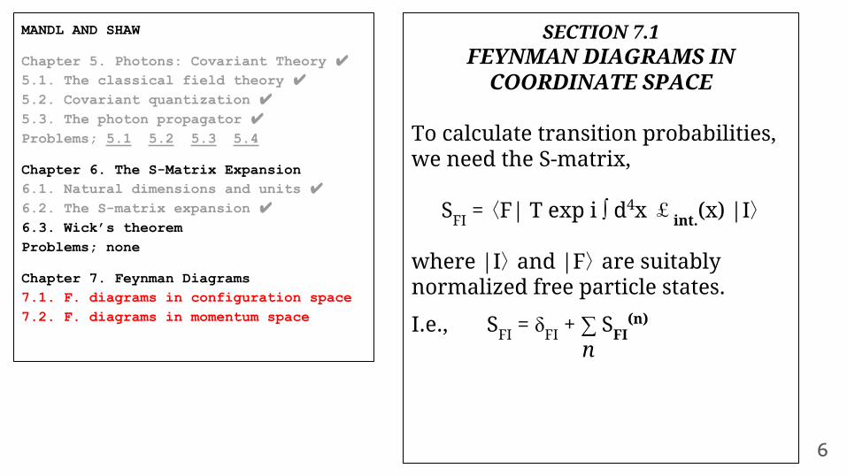
MANDL AND SHAW

Chapter 5. Photons: Covariant Theory5.1. The classical field theory ✔5.2. Covariant quantization ✔5.3. The photon propagatorProblems; 5.1 5.2 5.3 5.4

Chapter 6. The S-Matrix Expansion6.1. Natural Dimensions and Units ✔6.2. The S-matrix expansion ✔6.3. Wick’s theoremProblems; none

1

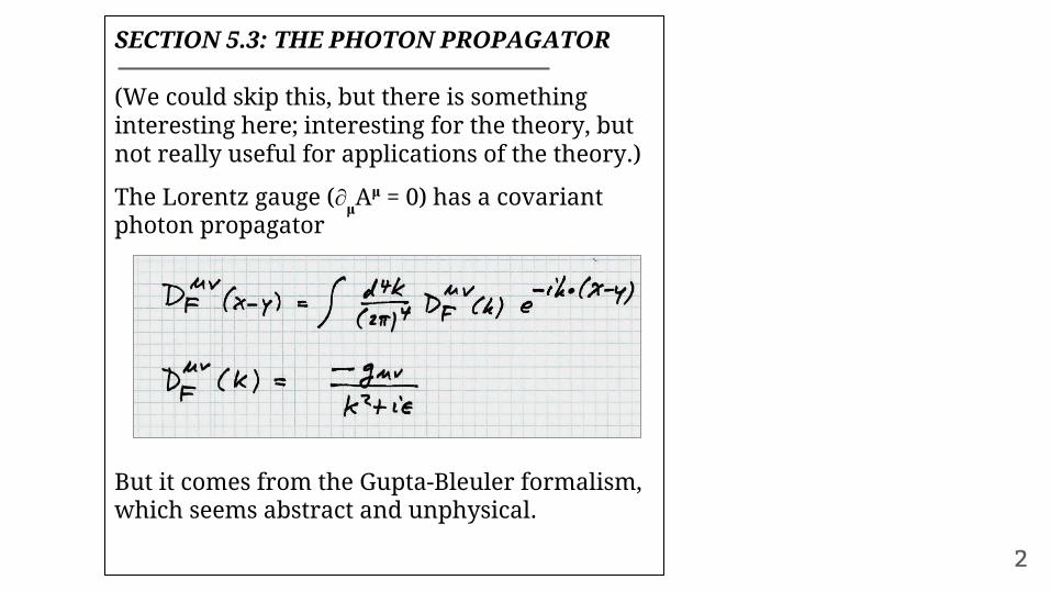
SECTION 5.3: THE PHOTON PROPAGATOR

(We could skip this, but there is something interesting here; interesting for the theory, but not really useful for applications of the theory.)

The Lorentz gauge (∂μAμ = 0) has a covariant

photon propagator

But it comes from the Gupta-Bleuler formalism, which seems abstract and unphysical.

2

1

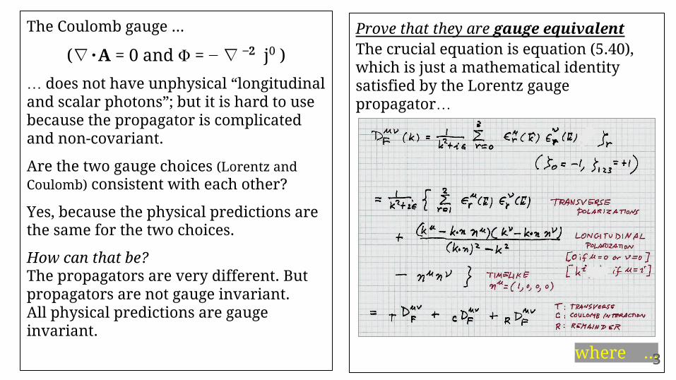
Prove that they are gauge equivalentThe crucial equation is equation (5.40),which is just a mathematical identity satisfied by the Lorentz gauge propagator…

where ...

The Coulomb gauge ...

(∇・A = 0 and Φ = − ∇ −2 j0 )

… does not have unphysical “longitudinal and scalar photons”; but it is hard to use because the propagator is complicated and non-covariant.

Are the two gauge choices (Lorentz and Coulomb) consistent with each other?

Yes, because the physical predictions are the same for the two choices.

How can that be?The propagators are very different. But propagators are not gauge invariant.All physical predictions are gauge invariant.

3

1

4

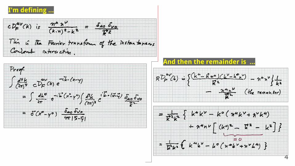
1 I'm defining ...

And then the remainder is ...

+

5

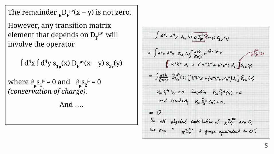
The remainder RDFμν(x − y) is not zero.

However, any transition matrix element that depends on DF

μν will involve the operator

∫ d4x ∫ d4y s1μ(x) DFμν(x − y) s2ν(y)

where ∂μs1μ = 0 and ∂μs2

μ = 0 (conservation of charge).

And ….

1

6

MANDL AND SHAW

Chapter 5. Photons: Covariant Theory ✔5.1. The classical field theory ✔5.2. Covariant quantization ✔5.3. The photon propagator ✔Problems; 5.1 5.2 5.3 5.4

Chapter 6. The S-Matrix Expansion6.1. Natural dimensions and units ✔6.2. The S-matrix expansion ✔6.3. Wick’s theoremProblems; none

Chapter 7. Feynman Diagrams7.1. F. diagrams in configuration space7.2. F. diagrams in momentum space

2 SECTION 7.1FEYNMAN DIAGRAMS IN

COORDINATE SPACE

To calculate transition probabilities, we need the S-matrix,

SFI = 〈F| T exp i ∫ d4x ￡int.(x) |I〉

where |I〉 and |F〉 are suitably normalized free particle states.

I.e., SFI = δFI + ∑ SFI(n)

n

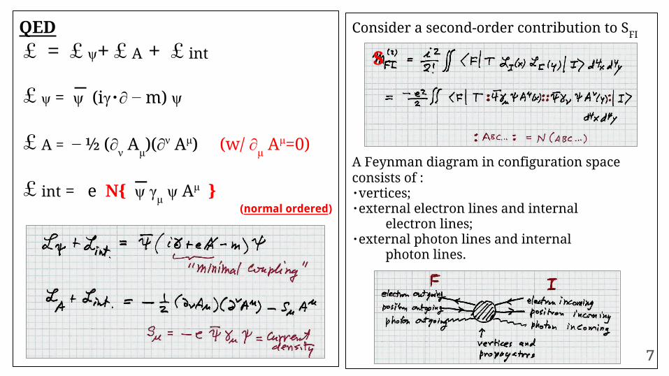
QED

￡ = ￡ψ+￡A + ￡int

￡ψ = ψ (iγ・∂ − m) ψ

￡A = − ½ (∂ν Aμ)(∂ν Aμ) (w/ ∂μ A

μ=0)

￡int = e N{ ψ γμ ψ Aμ }(normal ordered)

Consider a second-order contribution to SFI

A Feynman diagram in configuration space consists of :・vertices;・external electron lines and internal

electron lines;・external photon lines and internal

photon lines.

7

−

−

2

S

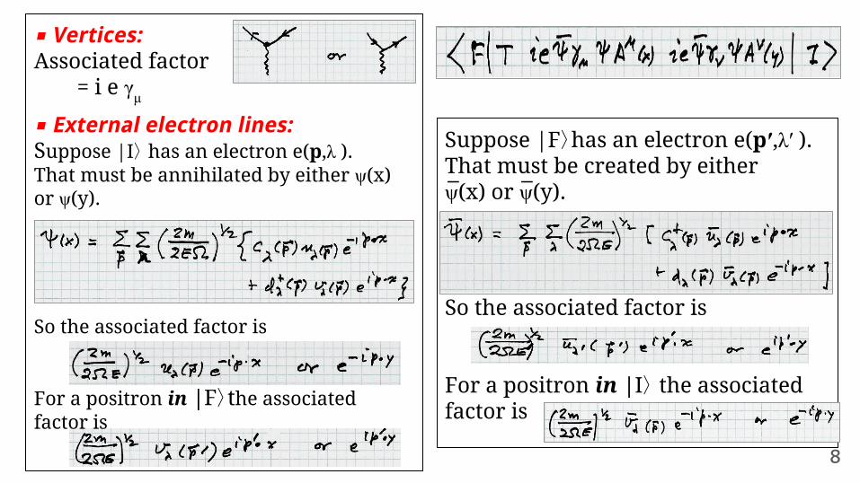
◾ Vertices:Associated factor

= i e γμ◾ External electron lines:Suppose |I〉 has an electron e(p,λ ).That must be annihilated by either ψ(x) or ψ(y).

So the associated factor is

For a positron in |F〉the associated factor is

8

2

Suppose |F〉has an electron e(p′,λ′ ).That must be created by eitherψ(x) or ψ(y).

So the associated factor is

For a positron in |I〉 the associated factor is

− −

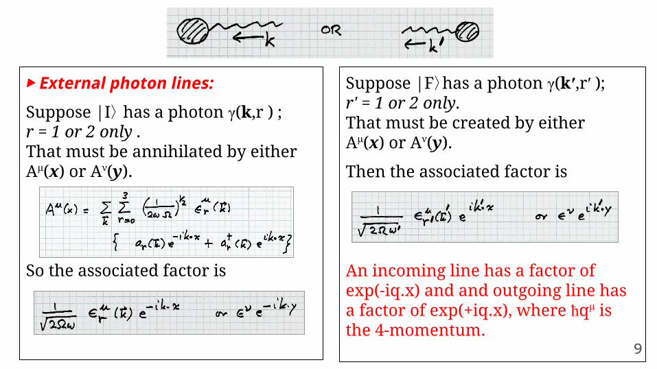
Suppose |F〉has a photon γ(k′,r′ );r' = 1 or 2 only.That must be created by eitherAμ(x) or Aν(y).

Then the associated factor is

An incoming line has a factor of exp(-iq.x) and and outgoing line has a factor of exp(+iq.x), where ħqμ is the 4-momentum.

▶ External photon lines:

Suppose |I〉 has a photon γ(k,r ) ;r = 1 or 2 only .That must be annihilated by either Aμ(x) or Aν(y).

So the associated factor is

9

2

10

▶ Internal electron lines:

Suppose Wick’s theorem requires the contraction ψ(x) ψ(y) ...

Then the associated factor is

SF(x − y) =

= (2π)−4∫ d4p SF(p) e−ip.(x − y)

−

▶ Internal photon lines:

Suppose Wick’s theorem requires the contraction Aμ(x) Aν(y) ...

Then the associated factor is

DFμν(x − y) =

= (2π)−4∫ d4k DFμν(k) e−ik.(x − y)

The other fields produce propagators.( Wick's theorem )

2