Mandatory management forecasts and lender expectations

1

Mandatory management forecasts and lender expectations

management

Andrew Ferguson, University of Technology, Sydney

Gabriel Pündrich, Bocconi University

August 2019

Abstract: The objective of this study is to broaden the existing literature on management forecasts

by examining how managers respond in terms of forecast characteristics once they are subject to

debt monitoring after project finance (PF) approval. Examining a large sample of mandatory

management forecasts of quarterly expenditure disclosed by early stage mining companies, we

find PF approval results in managers increasing overestimates of cash outflows or creating ‘budget

slack’. This is consistent with forecasts serving to manage expectations of lenders, signalling lower

risk of cost-overruns during the mine development and construction phase.

Keywords: Mandatory management forecasts, project finance, expectations management

*Corresponding author: Andrew Ferguson, email: [email protected]. We thank Ray Ball, John Core, Dan

Collins, Annita Florou, Jacquelyn Gillette, Amy Hutton, Claudia Imperatore, Alvis Lo, Suzie Noh, Valeria Marcia,

Georg Rickmann, Sugata Roychowdhury, Eric So, Andrew Sutherland, Suzie Noh, Rodrigo Verdi, Joseph Weber and

workshop participants at University of Iowa, Massachusetts Institute of Technology, Boston College, the 2018

International Accounting Symposium and the 2019 AAA conference for comments and suggestions. Finally, we thank

Matthew Grosse for assistance in compiling project finance data.

mailto:[email protected]

2

1. Introduction

Prior literature suggests expectations management is a primary motive for management

forecasts (Cotter, Tuna and Wysocki, 2006; Kato, Skinner and Kunimura, 2009). These studies

consider management forecasts used as a tool to manage the expectations of analysts and investors.

The objective of this study is to broaden the existing literature on management forecasts by

examining how managers forecast characteristics change in order to manage lender expectations.

To small mining companies without internal sources of finance, debt finance and ongoing support

of the lender is critical to developing high-risk projects, without which project development,

production and cash flow generation are not possible. To this extent, managers of small companies

have added incentives to manage (meet) expectations of project financiers and to manage forecasts

accordingly.

There is a paucity of research on the impact of leverage and more specifically the introduction

of lender monitoring on management forecasts, but prior studies suggest that greater leverage

should improve forecast accuracy owing to monitoring benefits (Hutton, Lee and Shu, 2012).

However, Hutton et al. (2012) suggest that managers in high information asymmetry settings

(where managers have an information advantage) may choose to issue less accurate forecasts

where they have incentives to do so (p. 1,218). We argue the receipt of Project Finance (PF)

approval changes managers’ incentives in terms of both forecast accuracy and bias such that

managers are motivated to meet the expectations of the new lender. It is likely that the new lender

is the target of this expectations management due to the limited analyst coverage of small mining

companies (Brown, Feigin and Ferguson, 2014) and high information asymmetry present in firms

previously all equity financed (Grossman and Hart, 1982).

Our study is motivated by the lack of prior research on the effects of introducing debt finance

into the capital structure of small firms and implications for forecast characteristics. We draw a

3

distinction between incentives of managers in large firms to manage expectations of analysts and

investors subject to prior study (Hutton, Lee, Shu, 2012; Cotter, Tuna and Wysocki, 2006; Kato,

Skinner and Kunimura, 2009) and those incentives of managers of small firms without a credit

history obtaining PF approval (Diamond, 1991). Accordingly, we might expect different forecast

characteristics in this alternative setting. We consider two research questions. Firstly, we examine

how PF approval impacts mandatory cash flow forecast accuracy and bias. Secondly, we consider

the likely duration of these effects.1

To examine these questions, we use a large sample of mandatory management forecasts of

expected future cash outflows related to operating activities payments disclosed by early-stage

(pre-production) mining firms known as Mining Exploration Entities (MEEs) in Australia.2

Notably, managers of MEEs are required to forecast only cash outflows related to operating

activities given their pre-production status. Although cash flow forecasts are a critical component

of successful investing (Goodman et al., 2013), they are not typically directly observable by

external stakeholders. Our setting is unique in that there are mandatory quarterly forecasts of

operating cash flows. Prior research has found it challenging to disentangle voluntary disclosure

choices and management forecast quality due to self-selection effects associated with managers

voluntarily providing earnings forecasts (e.g., Lennox and Park, 2006; Bamber et al., 2010;

Goodman et al., 2013; Lennox et al., 2011). The presence of mandatory management forecasts of

cash flows, however, allows us to consider forecast quality without potential concerns caused by

choice to provide management forecasts.

1 In a prior working paper version, Hutton et al. 2012 suggest that such incentives may play a more important role in

short term forecasts, as opposed to long-horizon forecasts. Our study considers short term forecasts 2 In this study, payment, cash payment, cash outflow, and cash expenditure are used interchangeably.

4

We hypothesize that MEEs obtaining PF coincides with the beginning of the mine

construction phase, where cost-overruns can be fatal, with frequent examples of failed projects

(BMO et al., 2014).3 Accordingly, we argue that to manage expectations of the lender, managers

will follow the old maxim ‘under-promise, over-deliver’ (Arnold 1986). In practical terms, this

suggests managers have incentives to bias forecasts towards providing overestimates of cash

outflows (under-promise) for which they can later meet (over-deliver). We further predict that

since PF is typically provided in tranches (similar to venture capital funding rounds, e.g., Sahlman,

1990, Gompers and Lerner, 1999), managers’ incentives to overestimate will be confined to the

period where debt drawdown occurs. This is because managers must meet project development

and construction milestones in order to secure a drawdown of further loan tranches to enable

project completion and the commencement of cash flow generation in the production phase

(Litvak, 2004).4 Accordingly, we suggest a time period where managing the expectations of the

lender is more likely. The possibility that managers may prefer less accurate short-term forecasts

should they be incentivized to do so is consistent with suggestions in Hutton et al., (2012).

Using a sample of in excess of 24,000 Appendix 5B filings over the period from July 1996 to

2014, we find that post-PF approval, manager’s exhibit increased the propensity to create budget

slack (forecast overestimates) while the level of underestimation remains unchanged. Additionally,

in terms of duration of this effect, we find that budget slack is most pronounced in the 12 month

period following PF approval, a period corresponding with project debt tranche drawdown and

construction activity, suggesting that management are most concerned about managing lender

3 See, for example, the history of the Bulong Nickel Project.

4 The MEE setting features lower analyst following that may provide managers different incentives concerning

their forecasts (Jiang, 2008). Second, pre-production MEEs have high information asymmetry in an industry featuring

significant levels of project failure. Also, Australia is a low litigation environment, and there are no plaints of

misleading forecasts by MEEs suggesting low potential legal constraints (Baginski, Hassell, and Kimbrough, 2002).

5

expectations where further debt tranches are yet to be drawn down (the lender retains discretion as

to whether this is possible) to enable project construction completion. These results are robust to

controlling for selection effects using a propensity score matching approach. These findings shed

light on how managers respond in terms of forecast characteristics once they are subject to debt

monitoring (e.g., Daley and Vigeland, 1983; Demerjian and Owens, 2016). We interpret this as

evidence consistent with the use of forecasts to manage lender expectations and mitigate concerns

of cost overruns (Cotter, Tuna and Wysocki, 2006; Kato, Skinner and Kunimura, 2009).

Our setting has a number of other interesting features. Debt finance in the US includes public

and private sources. In Australia, however, there is no material public debt market, meaning the

main source of debt finance available to most mining projects is private debt.5 Further, our setting

features the mandated disclosure of point, rather than range forecast estimates. This contrasts with

prior US literature, which features a dominance of range estimates compared to point estimates

(Hutton, Lee and Shu, 2012). Lastly, we examine a setting featuring the existence of management

cost forecasts by small firms. This contrasts the prior literature which has a large firm focus and is

important owing to the suggestion that in settings where managers have a dominant information

set (high information asymmetry), may be incentivized to forecast differently to large firms

(Hutton, Lee and Shu, 2012). Further, prior literature has focused on earnings forecasts, whilst in

this study, we focus on management forecasts of cash outflows.

The remainder of this paper is organized as follows. Section 2 reviews the background and

develops the hypothesis. Section 3 contains the research design, while Section 4 contains the

results. Section 5 concludes.

2. Background and hypothesis

5 A small number of much larger global mining firms are able to access debt markets in the US or Europe, e.g., BHP.

6

According to BDO, the number of MEE’s listed on the ASX as of June 2018 is 705.6

Excluding foreign listings, the number of ASX listed companies as at June 30th, 2018 was 2012.7

Thus MEEs typically comprise around 35% of total ASX listed entities. More broadly, the minerals

industry accounts for over half of Australia’s export earnings. The objectives of MEEs are both

homogeneous and straightforward. MEEs raise money through IPO’s or SEOs, and after listing

(or raising seasoned equity) spend money on exploration activity to make economic resource

discoveries. They have simple structures typically with a board of 3-4 persons, which will include

a technical director (geologist). Usually, apart from a company secretary, they will have no other

employees. MEEs are not equity carve-outs, nor are they subsidiaries of larger mining companies.

MEEs typically survive by issuing common or ordinary equity to shareholders (there is no

preferred equity issued in this setting). Occasionally, MEEs will issue options over ordinary shares

which trade alongside the fully paid shares on the ASX. Investors are typically speculators who

are attracted to the high payoffs associated with any discovery and subsequent mine development.

The ASX requires MEEs with no product sales to file a quarterly cash flow report called an

“Appendix 5B” (an example of an Appendix 5B is provided in Appendix II). These filings are

required since January 18th, 1996, and have the objective of assisting the market in understanding

the extent to which the entity is achieving its goals by disclosing information about expenditures

and cash flow (ASX, 2002, para.7). Guidance Note 31 of the ASX listing rules states that MEEs

are classified as such since their ‘main business activity is expending funds on mineral exploration

and evaluation and have minimal product revenues.’ The Guidance Note defines a ‘material

mining project’ as one in which a listed entity or subsidiary has an economic interest (whether

6 ‘Beneath the Surface Junior Mining Outlook’; BDO Edition 6, November 2018. 7 ASX Market Statistics. https://www.asx.com.au/about/historical-market-statistics.htm#No%20of%20Companies

(Link accessed 20190527).

https://www.asx.com.au/about/historical-market-statistics.htm#No%20of%20Companies

7

alone or jointly with others), where that interest is, or is likely to be, material in the context of the

overall business operations or financial results of the entity and subsidiaries (on a consolidated

basis).8

5Bs are required to be filed periodically until an MEE enters production and after that applies

to the ASX for permission to file only quarterly activities reports.9 Under ASX Listing Rule 5.5,

Appendix 5Bs must be filed within one month of the end of each quarter (March, June, September,

and December). These filings apply to companies defined as MEEs by the ASX as distinct from

Mining Producing Entities (ASX Listing Rules, Chapter 19). Thus, 5B filings for MEEs and the

forecasts of cash expenditure contained therein are mandatory under ASX listing rules for liquidity

risk assessment purposes.10

A unique feature of the PF approvals in Australia is a precise time-stamp given to

announcements along with a price-sensitive flag under the ASX’s continuous disclosure

requirements. The price-sensitive flag is due to the materiality of PF approvals for MEEs. The

announcements nearly always contain the lender identity, and PF approvals are associated with

positive market reactions (Ferguson, Grosse and Lam, 2018). Despite the high-risk nature of

8 A similar rule applies to non-mining research and development (R&D) companies admitted based on ‘commitments

test’ on or after 1st September 1999 such as pharmaceuticals and biotech firms that are required to file additional cash

flow disclosure in the form of the Appendix 4C (4Cs). However, R&D firms are only required to file 4Cs for eight

quarters after admission to the official list in order to disclose whether cash raised in an IPO has been spent in a manner

consistent with the companies’ business objectives (ASX Listing Rule 4.10.19). The 4Cs can be contrasted with 5Bs

disclosed by MEEs since 4Cs do not require disclosure of forecasts of cash outflows. Thus, we examine only 5Bs that

are required since 7/1/1996 and are not constrained by a 2-year disclosure period limit. MEEs are viewed by the

Australian Stock Exchange (ASX) as being high risk and consequently are required to produce additional mandatory

management expenditure forecasts (5Bs) as part of their quarterly reporting requirements. Unlike prior studies of

mandatory forecasts (where the forecasts are not in the strictest sense mandatory; e.g., Kato et al., 2009), operating

cash flow forecasts in MEEs are fully mandated by the ASX, are produced quarterly. 9 When an MEE progresses to seeking PF, it is common for MEE’s to spin off or dispose of non-development project-

related exploration interests effectively becoming ‘single project.’ A good example is the recent spin-off of Ardea

Resources by Heron Resources before the PF’s of the Woodlawn Zinc-Copper Project in New South Wales. Ardea

Resources primarily contained Heron Resources Western Australian nickel exploration interests. 10 See “estimated or forecast cash payments” in Section 1.5, page 3, of Appendix II and “actual cash flow” in Section

1.2, page 1.

8

mining projects, good projects can generate substantial profit margins for MEEs. Occasionally,

lenders take equity positions in MEEs they finance, which, unlike in the US, is legal in Australia.

This is especially common for mezzanine, seed or bridge loans, which are provided before the

main PF.11 Further, project sponsors may obtain PF from non-bank sources such as dedicated

mining investment funds, joint venture participants (larger mining companies), export credit

agencies, or off-take counterparties.12 PF loans are subject to loan covenants and are secured loans

collateralized by all project assets (Gatti et al., 2013). The PF lender’s incentive to monitor the

MEE is operationalized through contractual devices such as covenants and collateral similar to

those provisions in commercial bank lending (Rajan and Winton, 1995). Further, the structure of

PF loan drawdowns typically occurs at the lender’s discretion, with the drawdown of subsequent

debt tranches (undrawn facilities) subject to stringent performance hurdles. One limitation of this

study is that covenants are not observable. Thus, in the case of covenants, their implications may

differ from general loan covenants explored in the literature given the very specific nature of the

assets, the scope for opportunistic behavior and the concentrated nature of economic and financial

risk inherent in PF arrangements (Dailami, and Hauswald, 2003).13

Another feature of the US debt finance setting is the presence of a sizeable portion of the

information-sensitive debt (publicly traded corporate bonds). In Australia, however, there is no

11 These much smaller facilities are routinely provided to fund the completion of bankable feasibility studies or pilot

process plant construction, for example. 12 Non-bank sources of project loans are discussed further in Ferguson, Grosse and Lam (2019). 13 Mines in Australia are rarely financed through public debt markets as there is no information sensitive (public) debt

market in Australia (one exception is Fortescue Metals financing of its Cloud Break Iron Ore project located in

Western Australia, where Fortescue tapped the US public debt market - Refer to FMG ASX announcement dated

14/08/2006). Instead, the vast majority of PF occurs through private debt arrangements. MEEs are at high risk with

mining projects exhibiting many high profile failures. For example, the Bulong Nickel project located in Western

Australia, which ‘defaulted on its senior secured notes when its new pressure acid leach technology did not work as

expected’ (Esty 2002, p.75). Further, capital investment projects are notoriously high risk with suggestions that ‘50%

by my estimate encounter big setbacks’ and ‘where it is possible worst-case forecasts are almost always too optimistic’

(Arnold, 1986). Thus, in this high information asymmetry setting, management reputation and credibility are likely to

be important to lenders (Diamond, 1991).

9

active corporate bond market, meaning the primary source of debt finance available to most mining

projects is private debt.14

The relation between financing and forecast bias

Prior literature has shown that management forecasts are an important channel managers use

to convey information to equity (Lennox and Park, 2006; Skinner, 1994; Land and Lundholm,

2000; Cheng and Lo, 2006) and debt holders (Shivakumar et al., 2001; Jiang, 2008; Chin et al.,

2018; Bourveau et al., 2018). Other literature examines the reasons for management earnings

forecasts, arguing that expectations management is a primary motivation (Cotter, Tuna and

Wysocki, 2006; Kato, Skinner and Kunimura, 2009). This study draws on prior literature

suggesting the important role of expectations management in motivating management forecasts by

examining a different setting, featuring the existence of small firms obtaining PF approvals. These

firms lack credit history (Diamond, 1991) and exist in an information environment that features

low levels of analyst coverage (Brown, Feigin and Ferguson, 2014). Given these attributes of the

setting, we argue that managers will be primarily interested in fulfilling the expectations and the

new lender, who’s primary concern is cost-overruns and project failure.

Construction cost overruns occur where the actual costs of developing the project exceed

forecast capex and budget projections, resulting in the need to obtain additional funds to bring the

project into production and thus the cash generation phase. Forecast project capital costs are well

understood by the market from prior forecasts of capex appearing in feasibility studies. Cost

overruns in the construction phase can be fatal in MEEs (BMO et al., 2014), potentially

constituting an event of default and allowing the bank to terminate the facility agreement making

the existing financing due and payable (usually resulting in bankruptcy for MEEs). Consequently,

14 A small number of much larger global mining firms can access debt markets in the US or Europe, e.g., BHP,

Anaconda Nickel.

10

we argue managers of MEEs have incentives to overestimate forecast expenditures during the

construction phase to reassure the new lender and the equity market that cost-overruns are not an

issue for the project. Such signaling from managers is likely to be of added importance given the

significant adverse selection and moral hazard problems lenders and investors face in this sector

(Akerlof 1978).15

Prior to production commencement, MEE’s generate no internal funds, with banks providing

loans to firms with by and large no prior credit history (Diamond, 1991). 16,17 Arguments that

managers are incentivized to issue cost forecast overestimates to avoid cost-overruns are consistent

with assertions in Hutton et al. (2012). They suggest that managers in high information asymmetry

settings (where managers have an information advantage) may choose to issue less accurate

forecasts where they have incentives to do so (p. 1,218). Consistent with this argument, we suggest

this different setting is one where different forecast characteristics may result and pose the

following hypothesis in relation to managers incentives to overestimate future cash outflows after

obtaining PF as follows:

H1: Management forecasts will overestimate forecast cash payments related to operating

activities after PF is obtained.

Financing and the timing of forecast bias

15 The PF is associated with higher market value and is explored by Ferguson, Grosse and Lam (2019). 16 Another source of information on project construction is through the quarterly report of activities, where the progress

of project development are qualitatively described. However, the Appendix 5Bs are the only source of quantitative

assurance of progress on project development, which given the high level of information asymmetry, is likely to be of

added importance to both equity and debt market participants. 17 The role of intermediaries who finance early-stage firms and the ex-ante due diligence and monitoring activities

associated with the financing provided has been examined in venture capitalists (Chan, 1983), commercial banks

(Diamond, 1991) and private placement investors (Hertzel and Smith, 1993). These studies have shown how these

investments are possible to be accomplished in settings with substantial information asymmetry. Lastly, Ali et al.,

(2018) suggest that that firms use capital expenditure forecasts as a commitment mechanism to reduce contracting

costs with creditors.

11

Our second hypothesis relates to the timing of overestimates. Consistent with prior discussion,

PF approval for MEEs marks the beginning of the project development phase for MEEs possessing

other statutory approvals that are then able to commence mine construction activities.18 Like

venture capital funding rounds, PF debt tranches are typically staged investments, where the lender

makes available subsequent debt tranches to the borrower, conditional upon certain performance

hurdles being achieved (Sahlman, 1990, Gompers and Lerner, 1999). Prior theoretical signaling

literature identifies staged investment alternatives in the financing small of firms (Litvak, 2004,

Kim and Wagman, 2016). They identify the negative signaling risks associated with an investor

or venture capitalist (in this case a lender) not choosing to make a subsequent investment.

Similar to other research and development focused firms, MEEs are highly dependent on

meeting each hurdle concerning individual debt tranches to enable construction to continue to

completion. Thus, we argue the period of overestimation will coincide with the time between PF

approval and final tranche drawdown. We estimate this period coincides with construction

timelines, being approximately 12 months following PF approval. Thus we pose our second

hypothesis:

H2: Management forecasts will overestimate forecast cash payments related to operating

activities in the first year after the loan.

3. Research Design

3.1 Model specification

To examine H1, we estimate the following regression:

18 Another factor that may also influence forecasts is covenants. However, one limitation in our study is that covenants

are not observable, and its implications may differ from general loans primarily explored in the literature given the

very specific nature of the assets, the scope for opportunistic behavior and the concentrated nature of economic and

financial risk inherent in project finance (Dailami, and Hauswald, 2003).

12

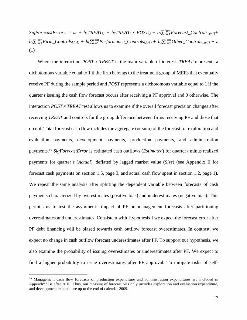
SigForecastErrori,t = αt + b1TREATi,t + b2TREATt x POSTi,t + bk∑𝑖=1𝑖=𝑛Forecast_Controlsi,(t-1)+

bk∑𝑖=1𝑖=𝑛Firm_Controlsi,(t-1) + bk∑𝑖=1

𝑖=𝑛Performance_Controlsi,(t-1) + bk∑𝑖=1𝑖=𝑛Other_Controlsi,(t-1) + ε

(1)

Where the interaction POST x TREAT is the main variable of interest. TREAT represents a

dichotomous variable equal to 1 if the firm belongs to the treatment group of MEEs that eventually

receive PF during the sample period and POST represents a dichotomous variable equal to 1 if the

quarter t issuing the cash flow forecast occurs after receiving a PF approval and 0 otherwise. The

interaction POST x TREAT test allows us to examine if the overall forecast precision changes after

receiving TREAT and controls for the group difference between firms receiving PF and those that

do not. Total forecast cash flow includes the aggregate (or sum) of the forecast for exploration and

evaluation payments, development payments, production payments, and administration

payments.19 SigForecastError is estimated cash outflows (Estimated) for quarter t minus realized

payments for quarter t (Actual), deflated by lagged market value (Size) (see Appendix II for

forecast cash payments on section 1.5, page 3, and actual cash flow spent in section 1.2, page 1).

We repeat the same analysis after splitting the dependent variable between forecasts of cash

payments characterized by overestimates (positive bias) and underestimates (negative bias). This

permits us to test the asymmetric impact of PF on management forecasts after partitioning

overestimates and underestimates. Consistent with Hypothesis I we expect the forecast error after

PF debt financing will be biased towards cash outflow forecast overestimates. In contrast, we

expect no change in cash outflow forecast underestimates after PF. To support our hypothesis, we

also examine the probability of issuing overestimates or underestimates after PF. We expect to

find a higher probability to issue overestimates after PF approval. To mitigate risks of self-

19 Management cash flow forecasts of production expenditure and administration expenditures are included in

Appendix 5Bs after 2010. Thus, our measure of forecast bias only includes exploration and evaluation expenditure,

and development expenditure up to the end of calendar 2009.

13

selection bias associated with the characteristic of firms receiving PF, tests are re-run restricting

the sample only to firms receiving PF, and by using a propensity score matching approach.

To examine Hypothesis II (H2), we run the following regression:

SigForecastErrori,t = b0 + bk∑𝑘=1𝑘=4Y(k)Before_loan + bk∑𝑘=1

𝑘=4Y(k)After_Loan +

bk∑𝑖=1𝑖=𝑛Forecast_Controlsi,(t-1)+ bk∑𝑖=1

𝑖=𝑛Firm_Controlsi,(t-1) + bk∑𝑖=1𝑖=𝑛Performance_Controlsi,(t-1) +

bk∑𝑖=1𝑖=𝑛Other_Controlsi,(t-1) + ε (2)

To test H2, we rerun the regression in the first hypothesis after adding dummies of the firm-

years around the first loan. This is done by adding four dummies indicating each one of the four

years before the loan (Y4_Before_Loan, Y3_Before_Loan, Y2_Before_Loan, and

Y1_Before_Loan) and for each one of the five years after the loan (Y1_After_Loan, Y2_After_Loan,

Y3_After_Loan, and Y4_After_Loan). We expect the overestimation bias to be higher in the first

year after the loan (Y1_After_Loan). To examine H2, we examine whether management forecasts

increase overestimates during the high-risk project construction phase. For this test, we rerun Eq.

(2) after substituting the dependent variable by the yearly dispersion (standard deviation) of

SigForecastError as a measure of uncertainty on the assessment of forecast credibility. We repeat

the test to all the components involved in the estimation (e.g., actual cost, estimation,

overestimation, and underestimation). We expect the first year after PF approval (Y1_After_Loan)

will have a significant and positive association with the standard deviation (dispersion) of forecast

error and its components. We further discuss the validity of our measure of uncertainty by running

a time-series to examine the decrease in the autocorrelation between overestimation bias driven by

larger actual cost dispersion.

Control variables are based on prior studies investigating management forecasts and other

literature examining MEEs (e.g., Kato, Skinner and Kunimura, 2009; Ferguson and Pündrich,

2015). Apart from controlling for lagged forecast error, we include control variables categorized

14

into three groups: forecast characteristics (Forecast_Controls), firm controls (Firm_Controls), and

firm performance (Perfomance_Controls). Forecast_Controls control for the autocorrelation

forecast bias by including lagged forecast bias (SigForecastError(t-1)). We include such lag controls

because prior research (Kato et al., 2009) has found that forecast error is autocorrelated. We also

include the number of pages accompanying the 5B to control for standalone Appendix 5Bs or 5Bs

appended to quarterly activities reports.

Firm-level control variables (Firm_Controls) include firm size (Size) calculated as the 60-

days average market value in a distance of 2-months before the announcement. We include a

control variable for firm size since prior studies (Kato et al., 2009) find larger firms have less

optimistic forecasts possibly due to higher external discipline (they may be cross-listed on overseas

exchanges or may face greater political and regulatory scrutiny). Further, managers of larger firms

may bear relatively larger reputational costs. Cash burn rate (Cash_Burn_Rate) is included to

control for incentives in communicating forecast cash outflow underestimates due to the

restrictions on remaining cash balances. Cash_Burn_Rate is calculated as the inverse of the

number of quarter’s worth of expenditure activity remaining at the current cash spending rate.

Other variables included are the lagged amount of cash available in the firm in the quarter (Cash)

scaled by lagged market value (Size). We include the age of the company (Firm age) as the number

of days the firm has been listed on the ASX to control for skill in forecasting payments since older

firms will have more experience and therefore should result in a smaller forecast bias. To control

for ownership concentration, we include the ratio of shares owned by the top 20 shareholders in

the company (Top_20).20

20 Firms are required by ASX to disclose the top 20 shareholders in their annual reports.

15

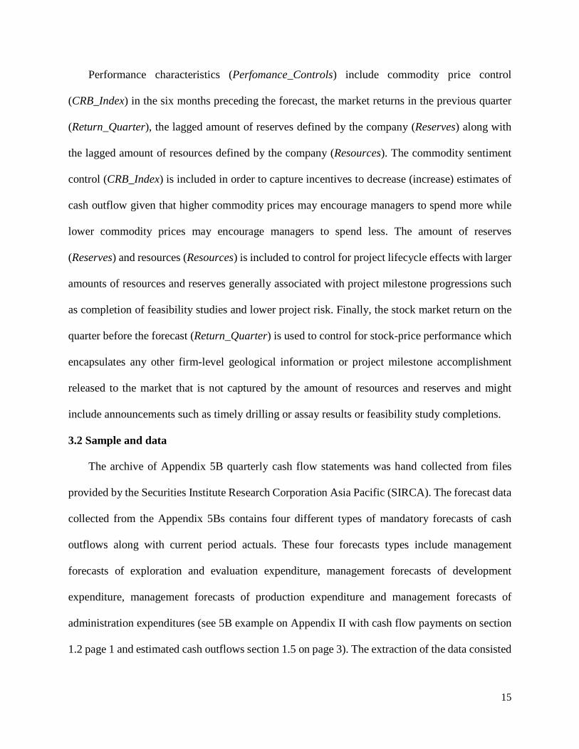
Performance characteristics (Perfomance_Controls) include commodity price control

(CRB_Index) in the six months preceding the forecast, the market returns in the previous quarter

(Return_Quarter), the lagged amount of reserves defined by the company (Reserves) along with

the lagged amount of resources defined by the company (Resources). The commodity sentiment

control (CRB_Index) is included in order to capture incentives to decrease (increase) estimates of

cash outflow given that higher commodity prices may encourage managers to spend more while

lower commodity prices may encourage managers to spend less. The amount of reserves

(Reserves) and resources (Resources) is included to control for project lifecycle effects with larger

amounts of resources and reserves generally associated with project milestone progressions such

as completion of feasibility studies and lower project risk. Finally, the stock market return on the

quarter before the forecast (Return_Quarter) is used to control for stock-price performance which

encapsulates any other firm-level geological information or project milestone accomplishment

released to the market that is not captured by the amount of resources and reserves and might

include announcements such as timely drilling or assay results or feasibility study completions.

3.2 Sample and data

The archive of Appendix 5B quarterly cash flow statements was hand collected from files

provided by the Securities Institute Research Corporation Asia Pacific (SIRCA). The forecast data

collected from the Appendix 5Bs contains four different types of mandatory forecasts of cash

outflows along with current period actuals. These four forecasts types include management

forecasts of exploration and evaluation expenditure, management forecasts of development

expenditure, management forecasts of production expenditure and management forecasts of

administration expenditures (see 5B example on Appendix II with cash flow payments on section

1.2 page 1 and estimated cash outflows section 1.5 on page 3). The extraction of the data consisted

16

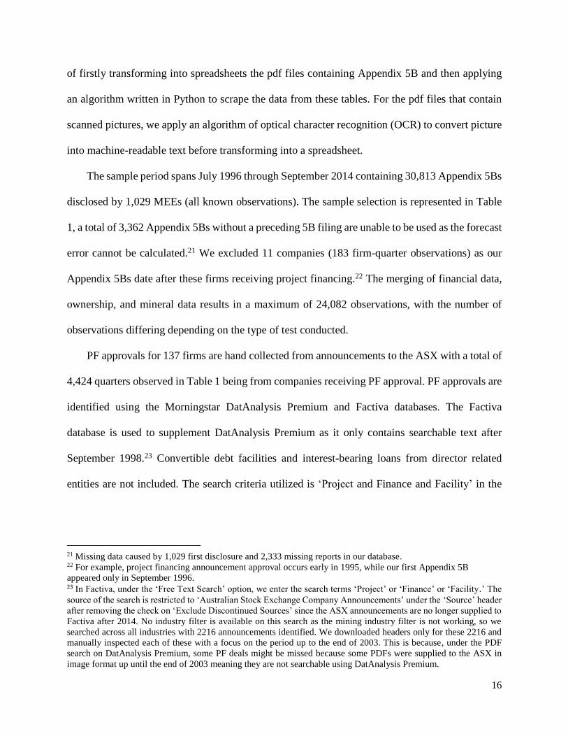
of firstly transforming into spreadsheets the pdf files containing Appendix 5B and then applying

an algorithm written in Python to scrape the data from these tables. For the pdf files that contain

scanned pictures, we apply an algorithm of optical character recognition (OCR) to convert picture

into machine-readable text before transforming into a spreadsheet.

The sample period spans July 1996 through September 2014 containing 30,813 Appendix 5Bs

disclosed by 1,029 MEEs (all known observations). The sample selection is represented in Table

1, a total of 3,362 Appendix 5Bs without a preceding 5B filing are unable to be used as the forecast

error cannot be calculated.21 We excluded 11 companies (183 firm-quarter observations) as our

Appendix 5Bs date after these firms receiving project financing.22 The merging of financial data,

ownership, and mineral data results in a maximum of 24,082 observations, with the number of

observations differing depending on the type of test conducted.

PF approvals for 137 firms are hand collected from announcements to the ASX with a total of

4,424 quarters observed in Table 1 being from companies receiving PF approval. PF approvals are

identified using the Morningstar DatAnalysis Premium and Factiva databases. The Factiva

database is used to supplement DatAnalysis Premium as it only contains searchable text after

September 1998.23 Convertible debt facilities and interest-bearing loans from director related

entities are not included. The search criteria utilized is ‘Project and Finance and Facility’ in the

21 Missing data caused by 1,029 first disclosure and 2,333 missing reports in our database. 22 For example, project financing announcement approval occurs early in 1995, while our first Appendix 5B

appeared only in September 1996. 23 In Factiva, under the ‘Free Text Search’ option, we enter the search terms ‘Project’ or ‘Finance’ or ‘Facility.’ The

source of the search is restricted to ‘Australian Stock Exchange Company Announcements’ under the ‘Source’ header

after removing the check on ‘Exclude Discontinued Sources’ since the ASX announcements are no longer supplied to

Factiva after 2014. No industry filter is available on this search as the mining industry filter is not working, so we

searched across all industries with 2216 announcements identified. We downloaded headers only for these 2216 and

manually inspected each of these with a focus on the period up to the end of 2003. This is because, under the PDF

search on DatAnalysis Premium, some PF deals might be missed because some PDFs were supplied to the ASX in

image format up until the end of 2003 meaning they are not searchable using DatAnalysis Premium.

17

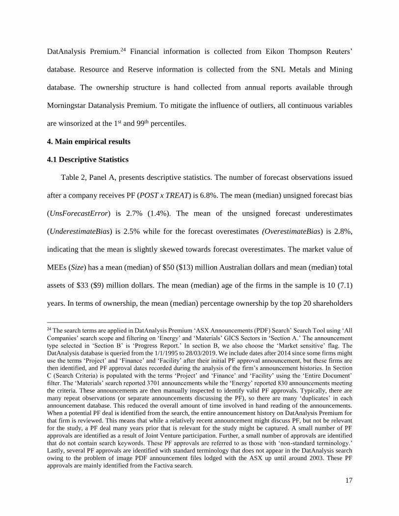
DatAnalysis Premium.24 Financial information is collected from Eikon Thompson Reuters’

database. Resource and Reserve information is collected from the SNL Metals and Mining

database. The ownership structure is hand collected from annual reports available through

Morningstar Datanalysis Premium. To mitigate the influence of outliers, all continuous variables

are winsorized at the 1st and 99th percentiles.

4. Main empirical results

4.1 Descriptive Statistics

Table 2, Panel A, presents descriptive statistics. The number of forecast observations issued

after a company receives PF (POST x TREAT) is 6.8%. The mean (median) unsigned forecast bias

(UnsForecastError) is 2.7% (1.4%). The mean of the unsigned forecast underestimates

(UnderestimateBias) is 2.5% while for the forecast overestimates (OverestimateBias) is 2.8%,

indicating that the mean is slightly skewed towards forecast overestimates. The market value of

MEEs (Size) has a mean (median) of $50 ($13) million Australian dollars and mean (median) total

assets of $33 ($9) million dollars. The mean (median) age of the firms in the sample is 10 (7.1)

years. In terms of ownership, the mean (median) percentage ownership by the top 20 shareholders

24 The search terms are applied in DatAnalysis Premium ‘ASX Announcements (PDF) Search’ Search Tool using ‘All

Companies’ search scope and filtering on ‘Energy’ and ‘Materials’ GICS Sectors in ‘Section A.’ The announcement

type selected in ‘Section B’ is ‘Progress Report.’ In section B, we also choose the ‘Market sensitive’ flag. The

DatAnalysis database is queried from the 1/1/1995 to 28/03/2019. We include dates after 2014 since some firms might

use the terms ‘Project’ and ‘Finance’ and ‘Facility’ after their initial PF approval announcement, but these firms are

then identified, and PF approval dates recorded during the analysis of the firm’s announcement histories. In Section

C (Search Criteria) is populated with the terms ‘Project’ and ‘Finance’ and ‘Facility’ using the ‘Entire Document’

filter. The ‘Materials’ search reported 3701 announcements while the ‘Energy’ reported 830 announcements meeting

the criteria. These announcements are then manually inspected to identify valid PF approvals. Typically, there are

many repeat observations (or separate announcements discussing the PF), so there are many ‘duplicates’ in each

announcement database. This reduced the overall amount of time involved in hand reading of the announcements.

When a potential PF deal is identified from the search, the entire announcement history on DatAnalysis Premium for

that firm is reviewed. This means that while a relatively recent announcement might discuss PF, but not be relevant

for the study, a PF deal many years prior that is relevant for the study might be captured. A small number of PF

approvals are identified as a result of Joint Venture participation. Further, a small number of approvals are identified

that do not contain search keywords. These PF approvals are referred to as those with ‘non-standard terminology.’

Lastly, several PF approvals are identified with standard terminology that does not appear in the DatAnalysis search

owing to the problem of image PDF announcement files lodged with the ASX up until around 2003. These PF

approvals are mainly identified from the Factiva search.

18

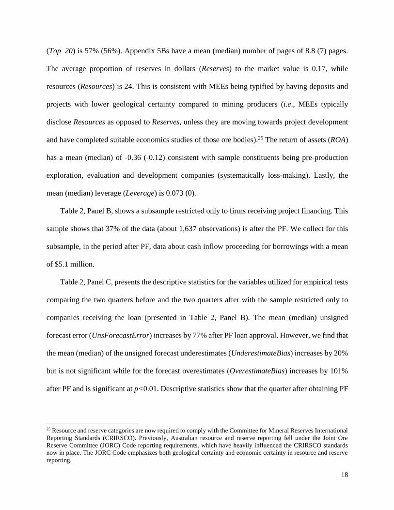
(Top_20) is 57% (56%). Appendix 5Bs have a mean (median) number of pages of 8.8 (7) pages.

The average proportion of reserves in dollars (Reserves) to the market value is 0.17, while

resources (Resources) is 24. This is consistent with MEEs being typified by having deposits and

projects with lower geological certainty compared to mining producers (i.e., MEEs typically

disclose Resources as opposed to Reserves, unless they are moving towards project development

and have completed suitable economics studies of those ore bodies).25 The return of assets (ROA)

has a mean (median) of -0.36 (-0.12) consistent with sample constituents being pre-production

exploration, evaluation and development companies (systematically loss-making). Lastly, the

mean (median) leverage (Leverage) is 0.073 (0).

Table 2, Panel B, shows a subsample restricted only to firms receiving project financing. This

sample shows that 37% of the data (about 1,637 observations) is after the PF. We collect for this

subsample, in the period after PF, data about cash inflow proceeding for borrowings with a mean

of $5.1 million.

Table 2, Panel C, presents the descriptive statistics for the variables utilized for empirical tests

comparing the two quarters before and the two quarters after with the sample restricted only to

companies receiving the loan (presented in Table 2, Panel B). The mean (median) unsigned

forecast error (UnsForecastError) increases by 77% after PF loan approval. However, we find that

the mean (median) of the unsigned forecast underestimates (UnderestimateBias) increases by 20%

but is not significant while for the forecast overestimates (OverestimateBias) increases by 101%

after PF and is significant at p<0.01. Descriptive statistics show that the quarter after obtaining PF

25 Resource and reserve categories are now required to comply with the Committee for Mineral Reserves International

Reporting Standards (CRIRSCO). Previously, Australian resource and reserve reporting fell under the Joint Ore

Reserve Committee (JORC) Code reporting requirements, which have heavily influenced the CRIRSCO standards

now in place. The JORC Code emphasizes both geological certainty and economic certainty in resource and reserve

reporting.

19

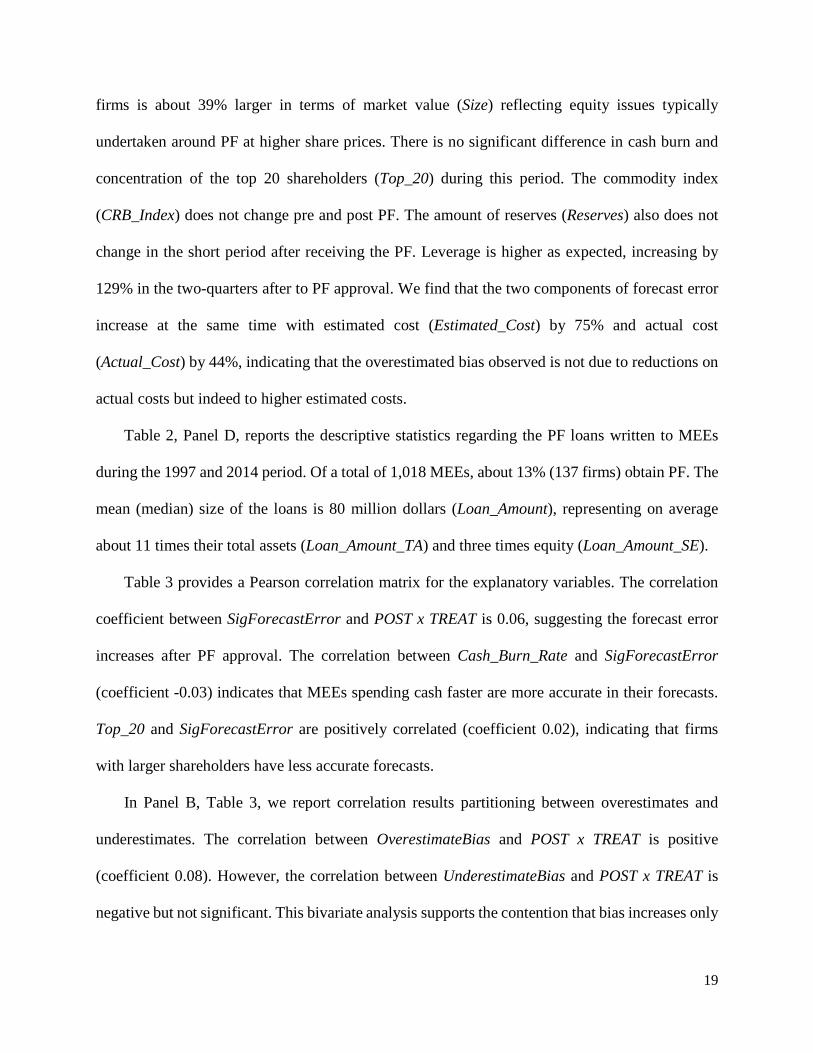
firms is about 39% larger in terms of market value (Size) reflecting equity issues typically

undertaken around PF at higher share prices. There is no significant difference in cash burn and

concentration of the top 20 shareholders (Top_20) during this period. The commodity index

(CRB_Index) does not change pre and post PF. The amount of reserves (Reserves) also does not

change in the short period after receiving the PF. Leverage is higher as expected, increasing by

129% in the two-quarters after to PF approval. We find that the two components of forecast error

increase at the same time with estimated cost (Estimated_Cost) by 75% and actual cost

(Actual_Cost) by 44%, indicating that the overestimated bias observed is not due to reductions on

actual costs but indeed to higher estimated costs.

Table 2, Panel D, reports the descriptive statistics regarding the PF loans written to MEEs

during the 1997 and 2014 period. Of a total of 1,018 MEEs, about 13% (137 firms) obtain PF. The

mean (median) size of the loans is 80 million dollars (Loan_Amount), representing on average

about 11 times their total assets (Loan_Amount_TA) and three times equity (Loan_Amount_SE).

Table 3 provides a Pearson correlation matrix for the explanatory variables. The correlation

coefficient between SigForecastError and POST x TREAT is 0.06, suggesting the forecast error

increases after PF approval. The correlation between Cash_Burn_Rate and SigForecastError

(coefficient -0.03) indicates that MEEs spending cash faster are more accurate in their forecasts.

Top_20 and SigForecastError are positively correlated (coefficient 0.02), indicating that firms

with larger shareholders have less accurate forecasts.

In Panel B, Table 3, we report correlation results partitioning between overestimates and

underestimates. The correlation between OverestimateBias and POST x TREAT is positive

(coefficient 0.08). However, the correlation between UnderestimateBias and POST x TREAT is

negative but not significant. This bivariate analysis supports the contention that bias increases only

20

in terms of overestimates but not underestimates after PF approval.26 In contrast, the coefficient

between Top_20 and OverestimateBias is positive (coefficient 0.03), suggesting larger

shareholders are associated with greater overestimates, at least on a bivariate level.

4.2 Multivariate analysis

Management forecasts after PF (Hypothesis H1)

Table 4, Panel A, presents regression results of tests examining the relation between forecast

bias PF approvals. Column (I) depicts the effect of PF approval (POST x TREAT) on the unsigned

or absolute value of the forecast error (UnsForecastError) (absolute value of estimated payments

for quarter t minus realized payments for quarter t, deflated by lagged market value (Size)). The

coefficient on POST x TREAT is positive (0.007) and significant at p<0.01, indicating that forecasts

become less accurate after PF approvals. In Column (II), we repeat the same test using a signed

variable, and the coefficient on POST x TREAT is again positive (0.005) and significant at

p<0.05.27 Notably, TREAT is significant in Columns I, III, and IV (p<0.05), indicating that on

average there are differences in forecast bias between the treatment and control group before firms

receive PF.

In Columns (III) and Column (IV) we partition the dependent variable between unsigned

forecast underestimates (UnderestimateBias: unsigned SigForecastError when the difference

between estimated and actual is negative – i.e., payments are more than expected) and unsigned

forecast overestimates (OverestimateBias: unsigned SigForecastError when the difference

between estimated and realized is positive – i.e., payments are less than expected or creation of

26 Multivariate analysis depicted in Table 4 fails to identify any association between larger shareholders proxied for

by the Top_20 and overestimates, suggesting that debt monitoring is of greater importance than large shareholder

monitoring in this setting. 27 We run the variance inflation factor to check for multicollinearity and find an average of 1.22 with no variable

higher than 1.56.

21

budget slack) respectively. POST x TREAT is not significant in Column (III), indicating that firms

do not issue more forecast underestimates after PF approvals. However, in Column (IV), we find

that the coefficient on POST x TREAT is positive (0.011, significant at p<0.01), suggesting an

increase in the overestimates. This is consistent with the hypothesis that forecasts bias increases,

but is asymmetric, with increasing forecast overestimates (OverestimateBias), and no difference

in the forecast underestimates (UnderestimateBias).

In terms of the coefficients on control variables, one interesting finding is the absence of any

significant results for Top_20. In contrast to bivariate results, in a multivariate setting, the

coefficients on Top_20 across columns (I)-(IV) (0.000, 0.004, 0.001, 0.000) are insignificant or

marginally insignificant, suggesting that larger shareholders have less monitoring impact than debt

providers at the PF approval stage. In terms of other control variables, commodity sentiment has

the opposite effect on each type of forecast error bias, being negative and insignificant for

UnderestimateBias but positive and significant for OverestimateBias. The amount of mineral

reserves (Reserves) is associated with higher SigForecastError and underestimates, while

resources (Resources) has a negative association. Higher quarterly returns are associated with both

smaller underestimates and overestimates. Thus, overall, we find multivariate evidence consistent

with H1.

To examine potential self-selection bias associated with firms receiving PF approvals and the

role of loan size as a determinant of overestimation bias, tests are re-run in Table 4, Panel B, after

restricting the sample only to firms receiving PF.28 Results are overall similar to those in Table 4,

28 Untabulated test, available upon request.

22

Panel A, suggesting the increase in overestimates is due to PF and not firm characteristics.29,30

Moreover, the interaction POST x TREAT x Loan_amount_SE is positive and significant in Column

IV, indicating that the bias is stronger when the loan represents a higher percentage of the firm

capital structure.

In untabulated results, we run a logistic regression examining the persistence of forecast bias

using a comprehensive sample with both firms receiving and not receiving PF loans before and

after the loan. While examining the determinants of underestimation bias, we find that POST x

TREAT is negative and significant, indicating that post-PF, MEEs are less prone to the

underestimation. However, when we switch the dependent variable to overestimated bias the same

variable is positive and significant, indicating that after PF, firms are more likely to provide

overestimates, consistent with Hypothesis I. Prior studies in the management forecast literature

have identified that forecast characteristic tend to persist or are autocorrelated. Together, this

evidence of persistence both in terms of underestimates and overestimates supports findings in

29 Some PF loan approvals are occasionally preceded by smaller seed or bridge loans. Seed loans are typically provided

for pre-development tasks such as feasibility study completion or pilot plant construction and operation used in

feasibility studies. In contrast, bridging finance is usually provided to MEEs having completed bankable feasibility

studies and requiring finance to commence project activity in the form of preliminary site works or to pay deposits on

capital equipment with long lead times to delivery. The association between seed and bridge loans and forecast bias

are considered in untabulated results. For this test, we include an additional dichotomous variable equal to one

indicating quarter forecasts after a seed or bridge loan is provided. We find similar results using this measure when

compared to actual PF loans examined in Table 4 with a positive relation between after bridge and overestimation but

not after seed and overestimation. This suggests an increase in forecast overestimates is not restricted to PF deals but

includes any smaller pre-development loans received before PF approval. This result is intuitive since good

stewardship of minor bridging loans commences the loan life cycle for these MEEs and thus contributes to the

development of the borrowers’ track record (Diamond, 1991). Thus, we interpret findings on bridge loans made to PF

loan recipients as being consistent with H1. 30 The dependent variable (SigForecastError) comprises four different types of mandatory forecasts of cash outflows

along with current period actuals. These four forecasts include management forecasts of exploration and evaluation

expenditure, management forecasts of development expenditure, management forecasts of production expenditure,

and management forecasts of administration expenditure (see 5B example in Appendix II). In untabulated results, we

examine the association between PF and forecast error by management forecast type (exploration and evaluation

expenditure, development expenditure, production expenditure, and administration expenditure). We find no

difference pre or post PF for overestimation of exploration bias or administration bias. This makes sense since

exploration and administration have been forecast by the firm for a long time before PF and also, are likely to be of

less interest to the lender. However, debt monitoring is likely to be focused on development and production payments,

which are the drivers of results.

23

Kato et al., who state that “These results are inconsistent with the reputation argument, which

predicts negative rather than positive autocorrelation in forecast bias.”31, 32

Management forecast timing (Hypothesis H2)

We hypothesize that MEEs face higher uncertainty during the high-risk construction phase

and have greater incentives to signal debtholders of lower risk of cost overruns by creating budget

slack, or to ‘under promise and over deliver’ as the project nears production (Rogers and Stocken,

2005). In Table 5, we examine cash flow estimates during the years after PF. In Column I, the

signed forecast error (SigForecastError) increases after PF. However, we find that overestimates

the increase in the first and second year as shown in Column (II) (Y1_After_Loan = 0.024, p<0.000,

Y2_After_Loan = 0.009, p<0.000) and not in the subsequent years. Results showing that

overestimation bias (Column II) is only higher in the first two years after PF approval is provided

consistent with the hypothesis that companies use budget slack for just a short period, providing

support for Hypothesis H2. A two year period after PF approval would see most MEEs already in

production. This result is graphically represented in Figure 1, where we plot estimates of firms

receiving PF approvals. It is possible to see that the greatest budget slack (overestimation) occurs

within the first four quarters (first year) after PF approval (quarter 0).

In Table 6, we consider whether management forecasts exhibit budget slack during high

uncertainty, proxied by the standard deviation of all the components involved in the estimation

31 In untabulated results, we also control for the lender identity in the PF loan approvals, enabling us to consider lender

characteristics such as industry leadership, specialization, and loan syndication. However, we observe no incremental

effects on overestimation from the leading project financier, alternative measures of specialists, or for projects funded

by syndicates. This may be due to the smaller loan size in PF deals to MEEs, compared to PF deals in the US, for

example. The smaller loan size suggests greater competition between potential lenders, with a large number of PF

participants to MEEs identified in Ferguson, Grosse and Lam (2018). 32 To deal with the self-selection associated with the characteristics of firms receiving PF, tests are re-run restricting

the sample only to firms receiving PF in untabulated results. Again, results are similar to those presented in the full

sample, providing further support that increases in the likelihood of overestimation are due to PF approvals and not

firm characteristics.

24

bias found in Table 4. In Columns (I) through Column (V), we find that the variable Y1_After_Loan

is significant and positive in all cases, consistent with our expectation that firms in the first year

following the loan are less homogeneous. This result provides some evidence that payments are

more heterogeneous in the first year and associated with higher dispersion. As time passes, the

MEEs need to manage lender expectations and create budget slack decreases as the project nears

production, risk decreases and an internal source of financing becomes available (see Figure 1).

Thus, budget slack is used for a short period of time where managers are incentivized to please

lenders who still maintain discretion around making available remaining debt tranches. This

supports the suggestions that managers create budget slack and are not driven merely by the

estimation difficulties during the construction period.

4.3 Additional tests and sensitivity analysis

Debt or equity signals?

Table 7 examines whether managers incentives are likely to be driven by debt or equity market

incentives. Column I shows that lagged cash from debt tranche drawdown (CashBorrowing) is

positive and significant (0.097, p<0.01) while lagged cash from share issuance (CashShares) is

positive but not significant. This result is consistent with managers creating budget slack to signal

lower risk of cost overruns motivated by credit market as opposed to equity market incentives. In

relation to Hypothesis 2, we include the variable CashBorrowingi,(t-2), calculated as the sum of

all debt tranches given up to 2 quarters before the overestimation is observed. We find the

interaction between CashSharesi,(t-1) x CashBorrowingi,(t-2) positive and significant (0.074,

p<0.05), indicating that as debt tranches are drawn-down, managers continue creating budget

slack. Column III and IV show the breakdown of SigForecastError and confirm that only

overestimations (positive SigForecastError) and not underestimations (negative

25

SigForecastError) increase after debt or equity is issued. These results further support the

interpretation that managers are motivated by credit market incentives.

Costs of overestimates and market reaction tests

In Table 8, we explore why all firms do not issue overestimates given the incentives to signal

lower risk of cost overruns to investors? Firstly, the incurrence of estimated greater cash outflows

by mining firms may be perceived positively by investors as it could be associated with the MEEs

increasing estimated spend due to an investment opportunity. Alternatively, an increase in

spending could signal cost overruns. In Table 8, Column I, we compute a mechanical model

calculated on the autocorrelation of the lagged four quarter to measure the surprise in the increase

of estimated cash outflow (ΔM_Estimated_Costt) of firms before receiving PF.

ΔM_Estimated_Costt is calculated by the subtraction of the estimated cash outflow in quarter t by

the predicted estimated cash outflow in quarter t provided by the model. Our results in Column I

show that an increase in estimated cash outflows is associated with higher market reactions

(ΔM_Estimated_Costt = 0.119, p<0.000), consistent with investors perceiving this increase as an

investment opportunity.

We also capture the investors’ perception of the overestimation of cash outflows by creating

the variable M_Predicted_Overspend, calculated as the difference between management forecasts

of payments for the quarter t+1 disclosed at quarter t and the predicted actual cost in t as a proxy

of expected payments in t+1.33 Our results in Column (I) indicate that the interaction of

33 We run four regressions to examine the autocorrelation between actual cost, estimated cost, and the forecast bias

(underestimate/overestimate). In untabulated results we find a significant autocorrelation between actual payments

(cash outflows) and its four (+, +, +, +) lagged quarters except for the third quarter with an adjusted R2 of 53% (Column

I). In the estimated payments we find a similar R2 although all lagged quarters are significant. Lastly, we find that the

expected bias in the next quarter is also a function of its prior four quarters but presents a smaller adjusted R2 of 16.1%

and 21% respectively. These results are consistent with the expectation that firms follow certain patterns in forecasts

and actual payments, and thus, investors recognize and unexpected forecast increase. The use of the mechanical model

is preferred as investors are likely to adjust their expectations given the higher systematic overestimate bias after

26

M_Predicted_Overspend and ΔEstimated_Costt is negative and significant (-0.171, p<0.05),

suggesting there is a negative market reaction when managers increase estimates if investors

believe spending should be lower than forecast by managers. These results are consistent in

Column (II) after including year fixed effect. These results indicate that an increase in spending

could signal greater cash burn than expected and is associated with greater risk of distress,

suggesting a cost that may provide an equilibrium associated with the choice to increase

overestimations.

Market reactions to the announcement of Appendix 5Bs are reported in Table 8. In Columns

(I) and (II) the variable Underestimated_Bias is negative and significant (-0.295, p<0.01; -0.214,

p<0.05; ), supporting our assumption that managers have incentives to avoid cost overruns by

overestimating expenses as equity markets perceive this as bad news.

Lifecycle effects on overestimates

We examine in Table 9 whether signals of overestimation is driven by lifecycle changes or

just from borrowing activities. We create the variable POST_DEVELi,t equal to 1 indicating when

a firm enters the development lifecycle (i.e., the amount of development cost is greater than

exploration and evaluation payments). Column IV shows that POST_DEVELi,t is positive but not

significant, indicating that the change of lifecycle does not alter the amount of overestimation

unless firms belong to the group receiving PF as the positive and significant interaction between

POST_DEVELi,t x TREATi,t. (0.009, p<0.05) demonstrates. This result supports suggestions that

overestimation increases due to capital raised from banks during the development phase and not

due to examples where equity finance is the sole project funding channel.

Overestimates and production commencement

project financing and is reasonable that the mechanical model better captures this adjustment as autocorrelations are

considered.

27

We examine in Table 10 whether signals of overestimations can predict positive project

milestones such as advancements into the production lifecycle or amount of receipts from early

ramp-up revenue. This table presents regression results of tests examining the determinants of

production costs (Column I and II) as a proxy for firms moving into production lifecycle and

receipts costs (Column III and IV) as a proxy for firms’ initial revenue generation. Our variable

of interest is the interaction Cumul_Overestimation, which is the cumulative average of

overestimations (OverestimateBias) up to the quarter before the production cost and revenue

disclosure in Appendix 5B. ProductionCost represents a continuous variable equal to the actual

expenditure in production (see Item 1.2 c in Appendix II) scaled by lagged market value (Size) and

Receipts represents a continuous variable equal to the actual receipts in quarter t (see Item 1.1in

Appendix II) scaled by lagged market value (Size). We find in Column I that the cumulative

overestimation is positive (0.158, p<0.05) and significant as in Column III (0.277, p<0.01) while

cumulative underestimation is not significant in Column II and IV. This result shows that higher

the cumulative signal in terms of overestimation after PF approval, the higher the likelihood of the

firm 1) advancing to producer status and 2) receives higher project ramp-up revenues. These results

suggest that signaling provided by managers through overestimates is effective in securing

remaining debt funding and progressing to producer status.

Determinants of debt drawdowns

Table 11 examines the debt market incentives in overestimated forecasts, given that there may

be similar debt market benefits (track record) in signals of managerial forecasts after PF approvals.

Accordingly, Column I shows that the lagged cumulative overestimation (Cumul_Overestimation)

is positive and significant (0.593, p<0.01) with the amount of cash received from debt drawdowns

(CashBorrowing) while the cumulative underestimation in Column II is not significant. This result

28

suggests that the way managers forecast and spend their cash flows may be associated with a good

track record. This result does not necessarily support that banks rely on public information for their

credit decisions, but, alternatively, that the forecast information used internally may be the same

benchmark disclosed to the public through cash flow forecasts. Finally, we repeat this test in

Column III by using a breakdown of overestimations by type of expense finding the driver of

overestimation is development expenses as predicted.

Endogeneity tests

Propensity Score Matching

Table 12 presents the propensity score matching used in controlling for the possibility that

other characteristics of firms obtaining PF might be associated with greater forecast overestimates.

Table 12 shows the first stage with an R2 of 19% and including 12,177 observations. Panel B shows

the estimates of the treatment group and control groups, where the difference in the treatment

group is significant at 1%. Panel C shows details common support indicating there is a high level

of common support. There are only three observations the propensity score did not align with the

propensity score of another observation in the opposite treatment category. The common support

is also shown graphically in Figure 3 depicting an overlap on propensity score corroborating with

our results shown on the propensity score matching output. Lastly, in Panel D we estimate the

effect of receiving PF on management forecasts using an inverse-probability-weighted (IPW)

treatment-effects estimator and find that the average treatment effect (ATE) is 0.018.

The regression using the weights calculated for the propensity score matching is presented on

Table 12 Panel E. Results corroborate with our main findings shown in Table 4, providing support

that the association between the overestimations and PF approval is not an endogenous one.

Managerial Overconfidence

29

It has been suggested these results may be consistent with a managerial overconfidence

interpretation. There are several reasons why this doesn’t make sense in this setting. Firstly,

managers face prolonged project life cycles. For example, it is typical for it to take a decade from

first mineral discovery to mine development (or even longer). Secondly, mineral exploration is

extremely high risk, with the chances of progressing from a greenfields geological target to a

profitable mine is 1 in 1000. If the target is redefined as a world-class deposit, the chances fall to

1 in 3333.34,35 Thirdly, mineral exploration is highly competitive with large numbers of MEEs

listed on the ASX and intense global competition for the exploration dollar, particularly from

Canada and Africa. Mineral explorers also have long track records of loss-making in an industry

known for its conservatism.

We conduct several tests which further decrease the likelihood of this interpretation. If

overconfidence is driven by an increase in cash via PF approval, we would observe that other prior

changes in cash that may be caused by non-routine project disposal (a non-pecking order related

avenue) are likewise associated with overestimation. However, in unreported analysis, we rule out

this explanation with overestimates only associated with debt and equity issuance (see Figure 2 for

graphical support of this evidence). Further, if large sums of money associated with PF were to

change managers behaviourally, we would observe differing (lower overconfidence) effects for

much smaller seed and bridge loans. However, controlling for seed and bridge loans makes no

34 Del Real, G, ‘Increasing the odds of Exploration Success. 13/01/2015) 35 Beatty, R, in ‘The declining discovery trend: People, Science or Scarcity? Society for Economic Geologists, April,

2010 suggests; Exploration is getting tougher. Despite increasing global exploration budgets year after year, it seems

that fewer and fewer new discoveries are being made. Why is this? Is it due to a lower quality of mineral explorationists

working globally, a dearth of new scientific methods being applied to discovery, or the increasing scarcity of mineral

deposits? It is most unlikely that there is a lower level of intellectual capital or science being applied to exploration.

My vote is therefore for scarcity.

30

difference to our primary results suggesting similar pecking order equity signaling effects apply to

small mezzanine type finance obtained, for example for feasibility study completions as to PF.

5. Conclusion

This study investigates whether managers create budget slack in expense forecasts driven by

debt market incentives (Cotter, Tuna and Wysocki, 2006; Kato, Skinner and Kunimura, 2009,

Hutton et al., 2012). Using a large sample of firms making mandatory forecasts of expenses, we

hypothesize MEE managers forecasts of cash outflows will feature more overestimates after PF

approvals. To examine the determinants of forecast bias, a dichotomous variable equal to one for

quarters after PF approval is utilized. Results are consistent with predictions in that after PF, the

cash outflow forecast bias increases, but only for overestimates, with no difference for

underestimates. Examining the timing of the overestimation, we find that managers are more likely

to create budget slack while debt tranches remain to be drawn, coinciding with the high-risk mine

construction phase. These results robust to using a propensity score matching approach.

This study is subject to limitations in the form of considering PF sources only in the form of

non-convertible loans, while we excluding instances of debt supplied to MEEs by director related

entities, which are typically of not great size. Secondly, we proxy for drawdowns using the

information contained in Appendix 5B, though obviously, this does not reflect precise tranche

drawdown dates, which are announced to the ASX relatively infrequently. Another possibility is

that management signaling takes place through construction updates in the Quarterly Activities

Report, which is it typically announced at the same time as the 5B. Thus, there may be qualitative

signaling of project progress in the activities report while the quantitative signaling appears in the

5B. We do not control for qualitative signals. Implications of the study more generally are limited

by the industry setting in Australia.

31

References

Akerlof, G. A. (1978). The market for “lemons”: Quality uncertainty and the market

mechanism. In Uncertainty in Economics (pp. 235-251). Academic Press.

Ali, A., Fan, Z., & Li, N. (2018). The role of capital expenditure forecasts in debt contracting.

Working Paper.

Arnold, J. Ill (1986). Assessing capital risk: you can’t be too conservative. Harvard Business

Review, 64, 113-121.

ASX (2002). Guidance note 23 appendix 4C. Australian Stock Exchange, March 2002.

Baginski, S. P., Hassell, J. M., & Kimbrough, M. D. (2002). The effect of legal environment

on voluntary disclosure: Evidence from management earnings forecasts issued in US and Canadian

markets. The Accounting Review, 77(1), 25-50.

Bamber, L. S., Jiang, J., & Wang, I. Y. (2010). What’s my style? The influence of top

managers on voluntary corporate financial disclosure. The Accounting Review, 85(4), 1131-1162.

Bartov, E., Givoly, D., & Hayn, C. (2002). The rewards to meeting or beating earnings

expectations. Journal of Accounting and Economics, 33(2), 173-204.

Beneish, M. D. 1999. Incentives and penalties related to earnings overstatements that violate

GAAP. The Accounting Review, 74 (4): 425-457.

BMO Capital Markets, Mayer Brown, SRK Consulting, EY (2014). Global mining guide

(2014). Mining journal. Stephens & George, Merthyr Tydfil, UK. ISBN: 978-0-9546893-9-1.

Bourveau, T., Stice, D. & Wang, R., (2018). Do managers strategically change their disclosure

before a debt covenant violation? Working paper.

Burgstahler, D., & Dichev, I. (1997). Earnings management to avoid earnings decreases and

losses. Journal of Accounting and Economics, 24(1), 99-126.

Bushman, R. M., & Wittenberg‐Moerman, R. (2012). The role of bank reputation in

“certifying” future performance implications of borrowers’ accounting numbers. Journal of

Accounting Research, 50(4), 883-930.

Brown, L. D., & Caylor, M. L. (2005). A temporal analysis of quarterly earnings thresholds:

propensities and valuation consequences. The Accounting Review, 80(2), 423-440.

Brown, P., Feigin, A., & Ferguson, A. (2014). Market reactions to the reports of a star resource

analyst. Australian Journal of Management, 39(1), 137–158.

Chan, Y. S. (1983). On the positive role of financial intermediation in allocation of venture

capital in a market with imperfect information. The Journal of Finance, 38(5), 1543-1568.

Cheng, Q., & K. Lo. (2006). Insider trading and voluntary disclosures. Journal of Accounting

Research, 44: 815-848.

Cheng, Q., Luo, T., & Yue, H. (2013). Managerial incentives and management forecast

precision. The Accounting Review, 88(5), 1575-1602.

Chin, C. L., Chen, M. H., & Yu, P. H. (2018). Does meeting analysts’ forecasts matter in the

private loan market? Journal of Empirical Finance, 48, 321-340.

32

Cotter, J., Tuna, I. and Wysocki, P. D. (2006), Expectations Management and Beatable

Targets: How Do Analysts React to Explicit Earnings Guidance? Contemporary Accounting

Research, 23: 593-624.

Dailami, M., & Hauswald, R. (2003). The emerging project bond market: covenant provisions

and credit spreads. The World Bank.

Daley, L. A., & Vigeland, R. L. (1983). The effects of debt covenants and political costs on

the choice of accounting methods: The case of accounting for R&D costs. Journal of Accounting

and Economics, 5, 195-211.

Degeorge, F., Patel, J., & Zeckhauser, R. (1999). Earnings management to exceed thresholds.

The Journal of Business, 72(1), 1-33.

Demerjian, P. R., & Owens, E. L. (2016). Measuring the probability of financial covenant

violation in private debt contracts. Journal of Accounting and Economics, 61(2-3), 433-447.

Diamond, D. W. (1984). Financial intermediation and delegated monitoring. The Review of

Economic Studies, 51(3), 393-414.

Diamond, D. W. (1991). Monitoring and reputation: the choice between bank loans and

directly placed debt. Journal of Political Economy, 99(4), 689-721.

Duchin, R. (2010). Cash holdings and corporate diversification. The Journal of Finance,

65(3), 955-992.

Esty, B. (2002). Returns on project‐financed investments: evolution and managerial

implications. Journal of Applied Corporate Finance, 15(1), 71-86.

Esty, B. C. (2004). Why study large projects? An introduction to research on project finance.

European Financial Management, 10(2), 213-224.

Ferguson, A., Grosse, M., & Lam, P. (2018). Determinants of market reactions to project

finance approvals. Working paper, University of Technology Sydney.

Ferguson, A., & Pündrich, G. (2015). Does industry specialist assurance of non-financial

information matter to investors?. Auditing: A Journal of Practice & Theory, 34(2), 121-146.

Gatti, S., Kleimeier, S., Megginson, W., & Steffanoni, A. (2013). Arranger certification in

project finance. Financial Management, 42(1), 1-40.

Gompers, P. and Lerner, J. 1999, ‘An analysis of compensation in the U.S. venture capital

partnership’, Journal of Financial Economics, vol. 51, pp. 3-44.

Goodman, T. H., Neamtiu, M., Shroff, N., & White, H. D. (2013). Management forecast

quality and capital investment decisions. The Accounting Review, 89(1), 331-365.

Grossman, S. J. and Hart, O. 1982, ‘Corporate financial structure and managerial incentives’,

The Economics of Information and Uncertainty, pp.107-140.

Hegazy, T. (2002). Computer-based construction project management (p. 398). Upper Saddle

River, NJ: Prentice Hall.

Hertzel, M., & Smith, R. L. (1993). Market discounts and shareholder gains for placing equity

privately. The Journal of finance, 48(2), 459-485.

Hutton, A. P., Lee, L. F., & Shu, S. Z. (2012). Do managers always know better? The relative

accuracy of management and analyst forecasts. Journal of Accounting Research, 50(5), 1217-1244.

33

Jiang, J. (2008). Beating earnings benchmarks and the cost of debt. The Accounting Review,

83(2), 377-416.

Kato, K., Skinner, D. J., & Kunimura, M. (2009). Management forecasts in japan: an empirical

study of forecasts that are effectively mandated. The Accounting Review, 84(5), 1575-1606.

Lang, M. H., & Lundholm, R. J. (2000). Voluntary disclosure and equity offerings: reducing

information asymmetry or hyping the stock?. Contemporary Accounting Research, 17(4), 623-

662.

Lennox, C. S., & Park, C. W. (2006). The informativeness of earnings and management’s

issuance of earnings forecasts. Journal of Accounting and Economics, 42(3), 439-458.

Lennox, C. S., Francis, J. R., & Wang, Z. (2011). Selection models in accounting research.

The Accounting Review, 87(2), 589-616.

Lerner, J., Shane, H., & Tsai, A. (2003). Do equity financing cycles matter? Evidence from

biotechnology alliances. Journal of Financial Economics, 67(3), 411-446.

Litvak, K. 2004, ‘Governance through exit: default penalties and walkaway options in venture

capital partnership agreements’, Willamette Law Review, vol. 40, pp. 771-812.

Megginson, W. L. (2010). Introduction to the special issue on project finance. Review of

Financial Economics: 19(2), 47-48.

Myers, S. C., & Majluf, N. S. (1984). Corporate financing and investment decisions when

firms have information that investors do not have. Journal of financial economics, 13(2), 187-221.

Rajan, R., & Winton, A. (1995). Covenants and collateral as incentives to monitor. The

Journal of Finance, 50(4), 1113-1146.

Rogers, J. L., & Stocken, P. C. (2005). Credibility of management forecasts. The Accounting

Review, 80(4), 1233-1260.

Shivakumar, L., Urcan, O., Vasvari, F. P., & Zhang, L. (2011). The debt market relevance of

management earnings forecasts: evidence from before and during the credit crisis. Review of

Accounting Studies, 16(3), 464.

Sahlman, W. A. 1990, ‘The structure and governance of venture capital organisations’,

Journal of Financial Economics, 27, 473-521.

Skinner, D. J. (1994). Why firms voluntarily disclose bad news. Journal of Accounting

Research, 32(1), 38-60.

Skinner, D. J. (1997). Earnings disclosures and stockholder lawsuits. Journal of Accounting

and Economics, 23(3), 249-282.

Trueman, B. (1986). Why do managers voluntarily release earnings forecasts?. Journal of

Accounting and Economics, 8(1), 53-71.

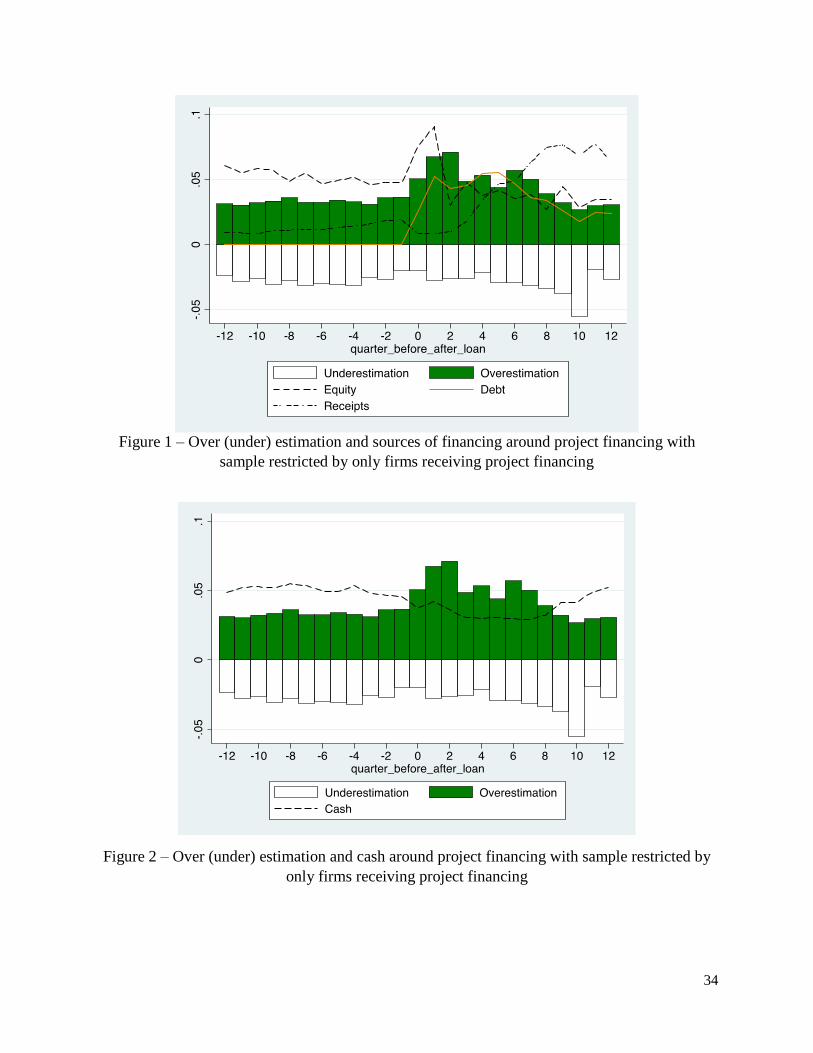
34

Figure 1 – Over (under) estimation and sources of financing around project financing with

sample restricted by only firms receiving project financing

Figure 2 – Over (under) estimation and cash around project financing with sample restricted by

only firms receiving project financing

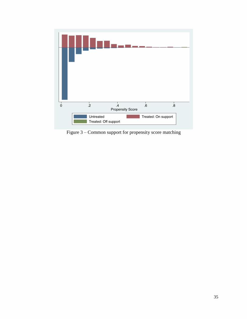
35

Figure 3 – Common support for propensity score matching

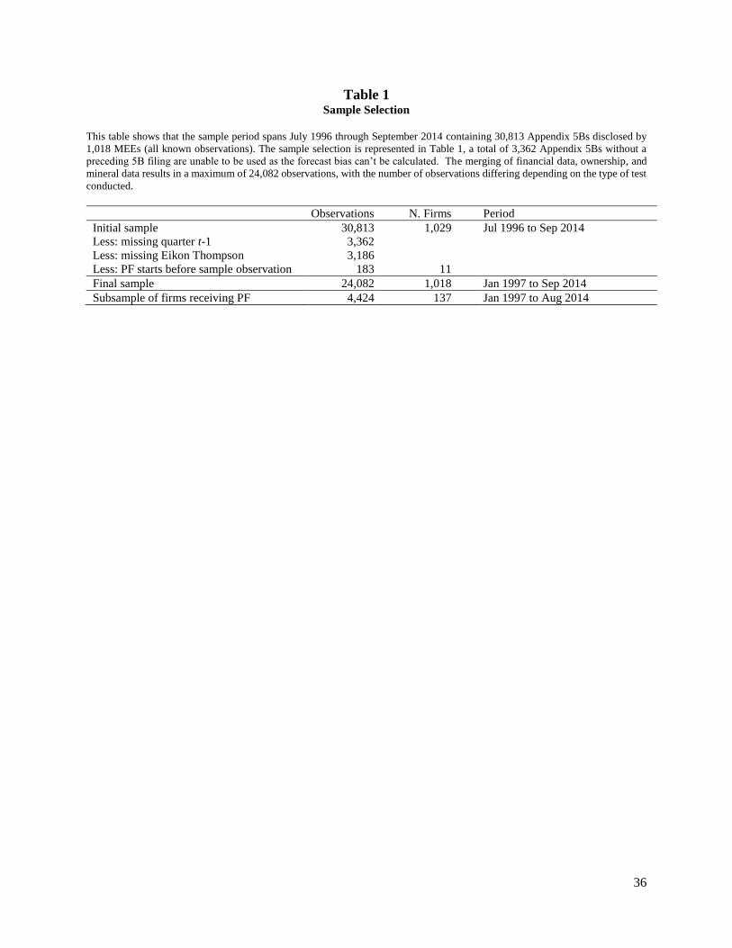
36

Table 1 Sample Selection

This table shows that the sample period spans July 1996 through September 2014 containing 30,813 Appendix 5Bs disclosed by

1,018 MEEs (all known observations). The sample selection is represented in Table 1, a total of 3,362 Appendix 5Bs without a

preceding 5B filing are unable to be used as the forecast bias can’t be calculated. The merging of financial data, ownership, and

mineral data results in a maximum of 24,082 observations, with the number of observations differing depending on the type of test

conducted.

Observations N. Firms Period

Initial sample 30,813 1,029 Jul 1996 to Sep 2014

Less: missing quarter t-1 3,362

Less: missing Eikon Thompson 3,186

Less: PF starts before sample observation 183 11

Final sample 24,082 1,018 Jan 1997 to Sep 2014

Subsample of firms receiving PF 4,424 137 Jan 1997 to Aug 2014

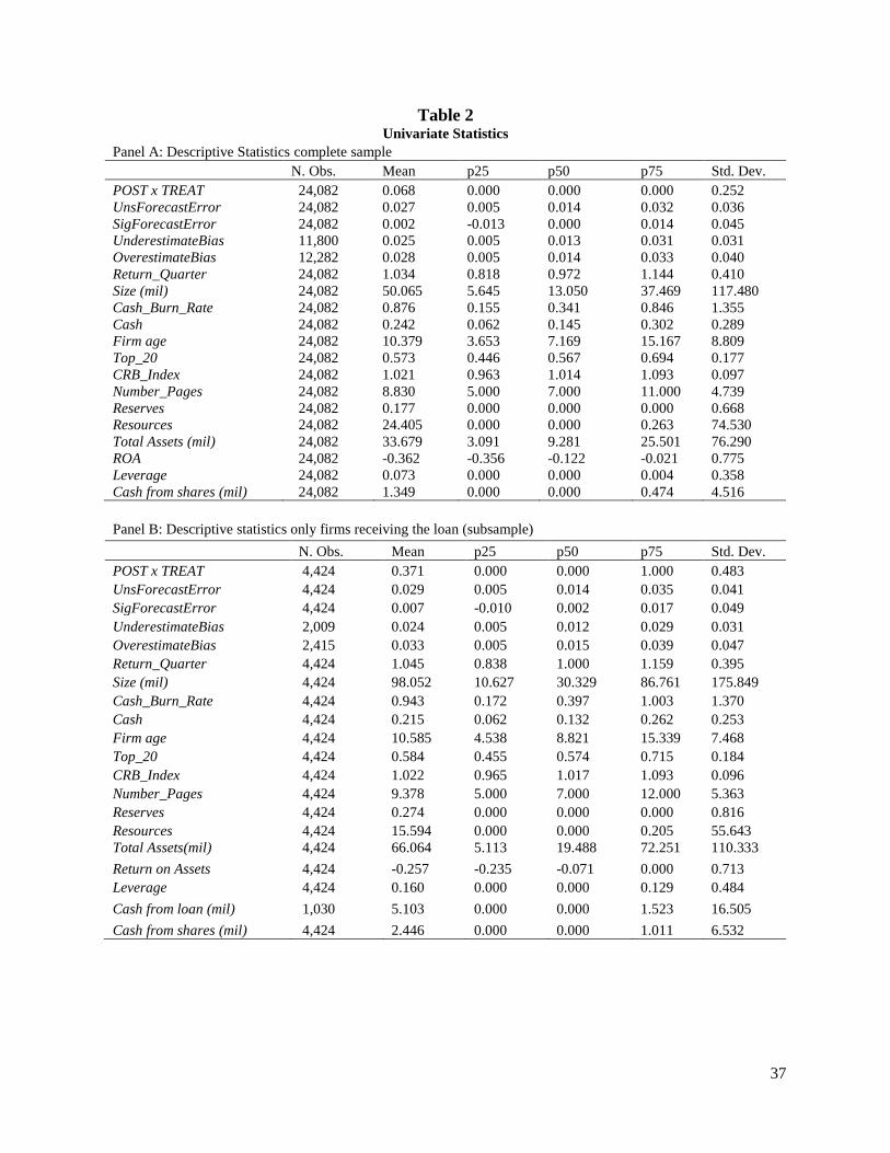
37

Table 2 Univariate Statistics

Panel A: Descriptive Statistics complete sample

N. Obs. Mean p25 p50 p75 Std. Dev.

POST x TREAT 24,082 0.068 0.000 0.000 0.000 0.252

UnsForecastError 24,082 0.027 0.005 0.014 0.032 0.036

SigForecastError 24,082 0.002 -0.013 0.000 0.014 0.045

UnderestimateBias 11,800 0.025 0.005 0.013 0.031 0.031

OverestimateBias 12,282 0.028 0.005 0.014 0.033 0.040

Return_Quarter 24,082 1.034 0.818 0.972 1.144 0.410

Size (mil) 24,082 50.065 5.645 13.050 37.469 117.480

Cash_Burn_Rate 24,082 0.876 0.155 0.341 0.846 1.355

Cash 24,082 0.242 0.062 0.145 0.302 0.289

Firm age 24,082 10.379 3.653 7.169 15.167 8.809

Top_20 24,082 0.573 0.446 0.567 0.694 0.177

CRB_Index 24,082 1.021 0.963 1.014 1.093 0.097

Number_Pages 24,082 8.830 5.000 7.000 11.000 4.739

Reserves 24,082 0.177 0.000 0.000 0.000 0.668

Resources 24,082 24.405 0.000 0.000 0.263 74.530

Total Assets (mil) 24,082 33.679 3.091 9.281 25.501 76.290

ROA 24,082 -0.362 -0.356 -0.122 -0.021 0.775

Leverage 24,082 0.073 0.000 0.000 0.004 0.358

Cash from shares (mil) 24,082 1.349 0.000 0.000 0.474 4.516

Panel B: Descriptive statistics only firms receiving the loan (subsample)


POST x TREAT 4,424 0.371 0.000 0.000 1.000 0.483

UnsForecastError 4,424 0.029 0.005 0.014 0.035 0.041

SigForecastError 4,424 0.007 -0.010 0.002 0.017 0.049

UnderestimateBias 2,009 0.024 0.005 0.012 0.029 0.031

OverestimateBias 2,415 0.033 0.005 0.015 0.039 0.047

Return_Quarter 4,424 1.045 0.838 1.000 1.159 0.395

Size (mil) 4,424 98.052 10.627 30.329 86.761 175.849

Cash_Burn_Rate 4,424 0.943 0.172 0.397 1.003 1.370

Cash 4,424 0.215 0.062 0.132 0.262 0.253

Firm age 4,424 10.585 4.538 8.821 15.339 7.468

Top_20 4,424 0.584 0.455 0.574 0.715 0.184

CRB_Index 4,424 1.022 0.965 1.017 1.093 0.096

Number_Pages 4,424 9.378 5.000 7.000 12.000 5.363

Reserves 4,424 0.274 0.000 0.000 0.000 0.816

Resources 4,424 15.594 0.000 0.000 0.205 55.643

Total Assets(mil) 4,424 66.064 5.113 19.488 72.251 110.333

Return on Assets 4,424 -0.257 -0.235 -0.071 0.000 0.713

Leverage 4,424 0.160 0.000 0.000 0.129 0.484

Cash from loan (mil) 1,030 5.103 0.000 0.000 1.523 16.505

Cash from shares (mil) 4,424 2.446 0.000 0.000 1.011 6.532

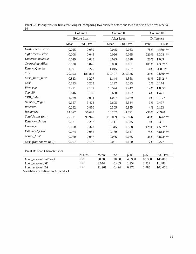
38

Panel C: Descriptives for firms receiving PF comparing two quarters before and two quarters after firms receive

PF Column I Column II Column III

Before Loan

After Loan

Difference

Mean Std. Dev. Mean Std. Dev. Perc. T-stat

UnsForecastError 0.025 0.039 0.045 0.053 78% 4.439***

SigForecastError 0.008 0.045 0.026 0.065 220% 3.308***

UnderestimateBias 0.019 0.025 0.023 0.028 20% 1.039

OverestimateBias 0.030 0.046 0.060 0.061 101% 4.38***

Return_Quarter 1.091 0.275 1.045 0.257 -4% -1.851*

Size 129.193 183.818 179.407 219.386 39% 2.649***

Cash_Burn_Rate 0.813 1.207 1.144 1.568 41% 2.542**

Cash 0.193 0.205 0.197 0.213 2% 0.174

Firm age 9.291 7.189 10.574 7.447 14% 1.885*

Top_20 0.616 0.166 0.638 0.172 4% 1.421

CRB_Index 1.029 0.091 1.027 0.089 0% -0.177

Number_Pages 9.357 5.428 9.605 5.584 3% 0.477

Reserves 0.292 0.850 0.305 0.855 4% 0.163

Resources 14.577 56.698 10.252 41.721 -30% -0.928

Total Assets (mil) 77.721 99.945 116.069 125.976 49% 3.626***

Return on Assets -0.121 0.257 -0.111 0.325 -8% 0.36

Leverage 0.150 0.323 0.345 0.558 129% 4.59***

Estimated_Cost 0.074 0.085 0.130 0.117 75% 5.814***

Actual_Cost 0.060 0.057 0.086 0.085 44% 3.873***

Cash from shares (mil) 0.057 0.137 0.061 0.150 7% 0.277

Panel D: Loan Characteristics


Loan_amount (million) 137 80.500 20.000 43.900 85.300 145.000

Loan_amount_SE 137 3.044 0.483 1.154 2.317 11.488

Loan_amount_TA 137 11.261 0.424 0.976 1.985 103.670

Variables are defined in Appendix I.

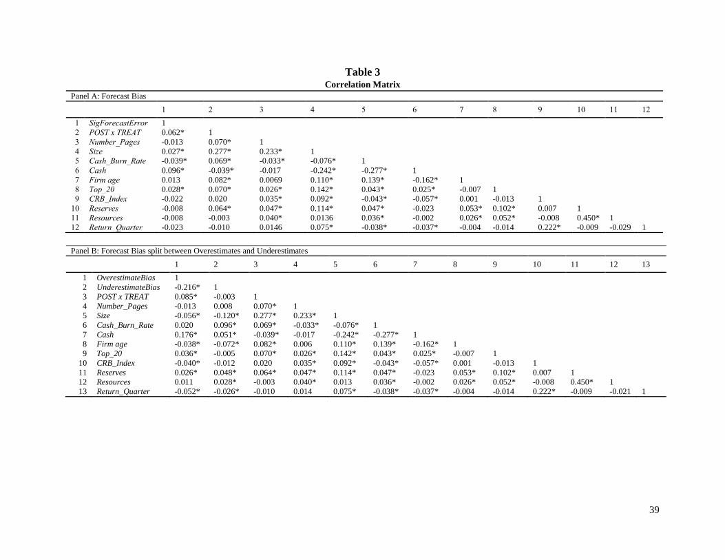
39

Table 3 Correlation Matrix

Panel A: Forecast Bias

1 2 3 4 5 6 7 8 9 10 11 12

1 SigForecastError 1 2 POST x TREAT 0.062* 1 3 Number_Pages -0.013 0.070* 1 4 Size 0.027* 0.277* 0.233* 1 5 Cash_Burn_Rate -0.039* 0.069* -0.033* -0.076* 1 6 Cash 0.096* -0.039* -0.017 -0.242* -0.277* 1 7 Firm age 0.013 0.082* 0.0069 0.110* 0.139* -0.162* 1 8 Top_20 0.028* 0.070* 0.026* 0.142* 0.043* 0.025* -0.007 1 9 CRB_Index -0.022 0.020 0.035* 0.092* -0.043* -0.057* 0.001 -0.013 1

10 Reserves -0.008 0.064* 0.047* 0.114* 0.047* -0.023 0.053* 0.102* 0.007 1 11 Resources -0.008 -0.003 0.040* 0.0136 0.036* -0.002 0.026* 0.052* -0.008 0.450* 1 12 Return_Quarter -0.023 -0.010 0.0146 0.075* -0.038* -0.037* -0.004 -0.014 0.222* -0.009 -0.029 1

Panel B: Forecast Bias split between Overestimates and Underestimates

1 2 3 4 5 6 7 8 9 10 11 12 13

1 OverestimateBias 1 2 UnderestimateBias -0.216* 1 3 POST x TREAT 0.085* -0.003 1 4 Number_Pages -0.013 0.008 0.070* 1 5 Size -0.056* -0.120* 0.277* 0.233* 1 6 Cash_Burn_Rate 0.020 0.096* 0.069* -0.033* -0.076* 1 7 Cash 0.176* 0.051* -0.039* -0.017 -0.242* -0.277* 1 8 Firm age -0.038* -0.072* 0.082* 0.006 0.110* 0.139* -0.162* 1 9 Top_20 0.036* -0.005 0.070* 0.026* 0.142* 0.043* 0.025* -0.007 1

10 CRB_Index -0.040* -0.012 0.020 0.035* 0.092* -0.043* -0.057* 0.001 -0.013 1 11 Reserves 0.026* 0.048* 0.064* 0.047* 0.114* 0.047* -0.023 0.053* 0.102* 0.007 1 12 Resources 0.011 0.028* -0.003 0.040* 0.013 0.036* -0.002 0.026* 0.052* -0.008 0.450* 1 13 Return_Quarter -0.052* -0.026* -0.010 0.014 0.075* -0.038* -0.037* -0.004 -0.014 0.222* -0.009 -0.021 1

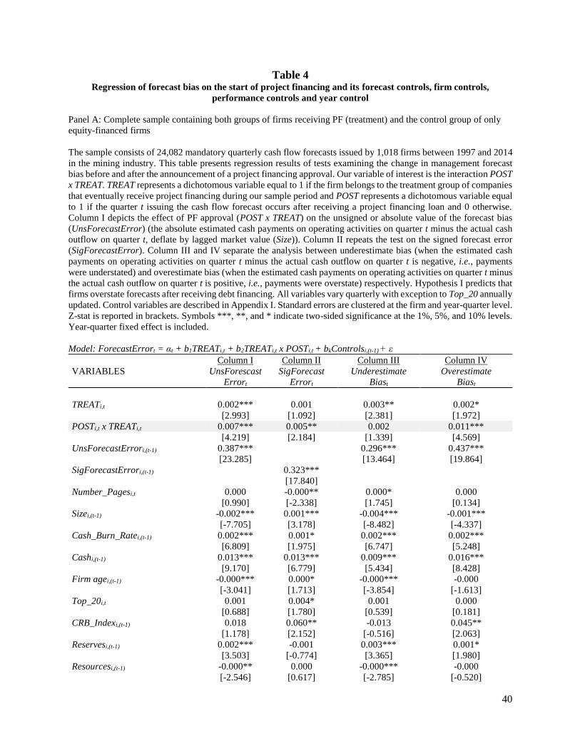
40

Table 4 Regression of forecast bias on the start of project financing and its forecast controls, firm controls,

performance controls and year control

Panel A: Complete sample containing both groups of firms receiving PF (treatment) and the control group of only

equity-financed firms

The sample consists of 24,082 mandatory quarterly cash flow forecasts issued by 1,018 firms between 1997 and 2014

in the mining industry. This table presents regression results of tests examining the change in management forecast

bias before and after the announcement of a project financing approval. Our variable of interest is the interaction POST

x TREAT. TREAT represents a dichotomous variable equal to 1 if the firm belongs to the treatment group of companies

that eventually receive project financing during our sample period and POST represents a dichotomous variable equal

to 1 if the quarter t issuing the cash flow forecast occurs after receiving a project financing loan and 0 otherwise.

Column I depicts the effect of PF approval (POST x TREAT) on the unsigned or absolute value of the forecast bias

(UnsForecastError) (the absolute estimated cash payments on operating activities on quarter t minus the actual cash

outflow on quarter t, deflate by lagged market value (Size)). Column II repeats the test on the signed forecast error

(SigForecastError). Column III and IV separate the analysis between underestimate bias (when the estimated cash

payments on operating activities on quarter t minus the actual cash outflow on quarter t is negative, i.e., payments

were understated) and overestimate bias (when the estimated cash payments on operating activities on quarter t minus

the actual cash outflow on quarter t is positive, i.e., payments were overstate) respectively. Hypothesis I predicts that

firms overstate forecasts after receiving debt financing. All variables vary quarterly with exception to Top_20 annually

updated. Control variables are described in Appendix I. Standard errors are clustered at the firm and year-quarter level.

Z-stat is reported in brackets. Symbols ***, **, and * indicate two-sided significance at the 1%, 5%, and 10% levels.

Year-quarter fixed effect is included.

Model: ForecastErrort = αt + b1TREATi,t + b2TREATi,t x POSTi,t + bkControlsi,(t-1) + ε

Column I Column II Column III Column IV

VARIABLES UnsForescast

Errort

SigForecast

Errort

Underestimate

Biast

Overestimate

Biast

TREATi,t 0.002*** 0.001 0.003** 0.002*

[2.993] [1.092] [2.381] [1.972]

POSTi,t x TREATi,t 0.007*** 0.005** 0.002 0.011***

[4.219] [2.184] [1.339] [4.569]

UnsForecastErrori,(t-1) 0.387*** 0.296*** 0.437***

[23.285] [13.464] [19.864]

SigForecastErrori,(t-1) 0.323***

[17.840]

Number_Pagesi,t 0.000 -0.000** 0.000* 0.000

[0.990] [-2.338] [1.745] [0.134]

Sizei,(t-1) -0.002*** 0.001*** -0.004*** -0.001***

[-7.705] [3.178] [-8.482] [-4.337]

Cash_Burn_Ratei,(t-1) 0.002*** 0.001* 0.002*** 0.002***

[6.809] [1.975] [6.747] [5.248]

Cashi,(t-1) 0.013*** 0.013*** 0.009*** 0.016***

[9.170] [6.779] [5.434] [8.428]

Firm agei,(t-1) -0.000*** 0.000* -0.000*** -0.000

[-3.041] [1.713] [-3.854] [-1.613]

Top_20i,t 0.001 0.004* 0.001 0.000

[0.688] [1.780] [0.539] [0.181]

CRB_Indexi,(t-1) 0.018 0.060** -0.013 0.045**

[1.178] [2.152] [-0.516] [2.063]

Reservesi,(t-1) 0.002*** -0.001 0.003*** 0.001*

[3.503] [-0.774] [3.365] [1.980]

Resourcesi,(t-1) -0.000** 0.000 -0.000*** -0.000

[-2.546] [0.617] [-2.785] [-0.520]

41

Return_Quarteri,(t-1) -0.005*** -0.002*** -0.004*** -0.006***

[-6.657] [-4.162] [-5.562] [-5.796]

Constant 0.053*** -0.023*** 0.078*** 0.037***

[10.661] [-3.827] [10.941] [6.742]

Observations 24,082 24,082 11,800 12,282

Year-quarter FE Yes Yes Yes Yes

Firm & Year-q Cluster Yes Yes Yes Yes

Adj. R-squared 0.237 0.138 0.222 0.260

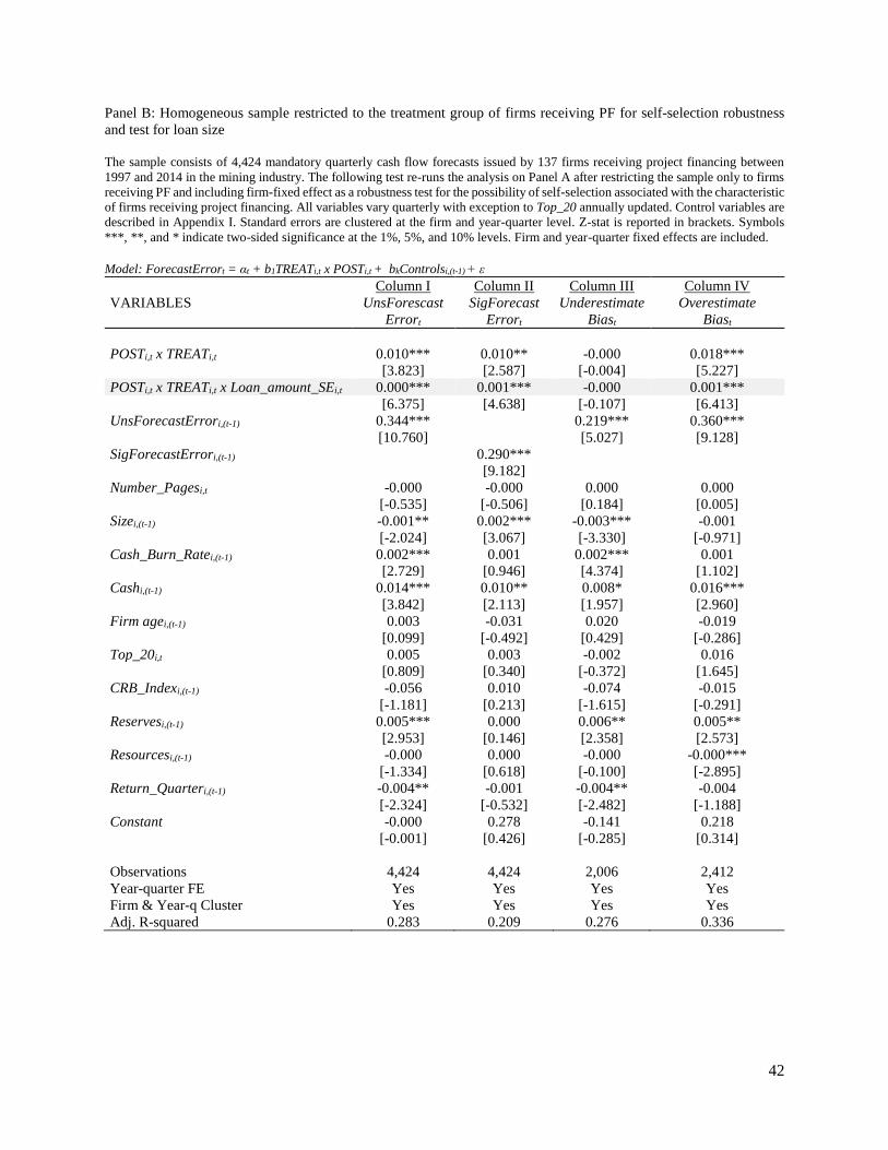
42

Panel B: Homogeneous sample restricted to the treatment group of firms receiving PF for self-selection robustness

and test for loan size

The sample consists of 4,424 mandatory quarterly cash flow forecasts issued by 137 firms receiving project financing between

1997 and 2014 in the mining industry. The following test re-runs the analysis on Panel A after restricting the sample only to firms

receiving PF and including firm-fixed effect as a robustness test for the possibility of self-selection associated with the characteristic

of firms receiving project financing. All variables vary quarterly with exception to Top_20 annually updated. Control variables are

described in Appendix I. Standard errors are clustered at the firm and year-quarter level. Z-stat is reported in brackets. Symbols

***, **, and * indicate two-sided significance at the 1%, 5%, and 10% levels. Firm and year-quarter fixed effects are included.

Model: ForecastErrort = αt + b1TREATi,t x POSTi,t + bkControlsi,(t-1) + ε



Errort

SigForecast

Errort

Underestimate

Biast

Overestimate

Biast

POSTi,t x TREATi,t 0.010*** 0.010** -0.000 0.018***

[3.823] [2.587] [-0.004] [5.227]

POSTi,t x TREATi,t x Loan_amount_SEi,t 0.000*** 0.001*** -0.000 0.001***

[6.375] [4.638] [-0.107] [6.413]


[10.760] [5.027] [9.128]


[9.182]

Number_Pagesi,t -0.000 -0.000 0.000 0.000

[-0.535] [-0.506] [0.184] [0.005]

Sizei,(t-1) -0.001** 0.002*** -0.003*** -0.001

[-2.024] [3.067] [-3.330] [-0.971]

Cash_Burn_Ratei,(t-1) 0.002*** 0.001 0.002*** 0.001

[2.729] [0.946] [4.374] [1.102]

Cashi,(t-1) 0.014*** 0.010** 0.008* 0.016***

[3.842] [2.113] [1.957] [2.960]

Firm agei,(t-1) 0.003 -0.031 0.020 -0.019

[0.099] [-0.492] [0.429] [-0.286]

Top_20i,t 0.005 0.003 -0.002 0.016

[0.809] [0.340] [-0.372] [1.645]

CRB_Indexi,(t-1) -0.056 0.010 -0.074 -0.015

[-1.181] [0.213] [-1.615] [-0.291]

Reservesi,(t-1) 0.005*** 0.000 0.006** 0.005**

[2.953] [0.146] [2.358] [2.573]

Resourcesi,(t-1) -0.000 0.000 -0.000 -0.000***

[-1.334] [0.618] [-0.100] [-2.895]

Return_Quarteri,(t-1) -0.004** -0.001 -0.004** -0.004

[-2.324] [-0.532] [-2.482] [-1.188]

Constant -0.000 0.278 -0.141 0.218

[-0.001] [0.426] [-0.285] [0.314]

Observations 4,424 4,424 2,006 2,412



Adj. R-squared 0.283 0.209 0.276 0.336

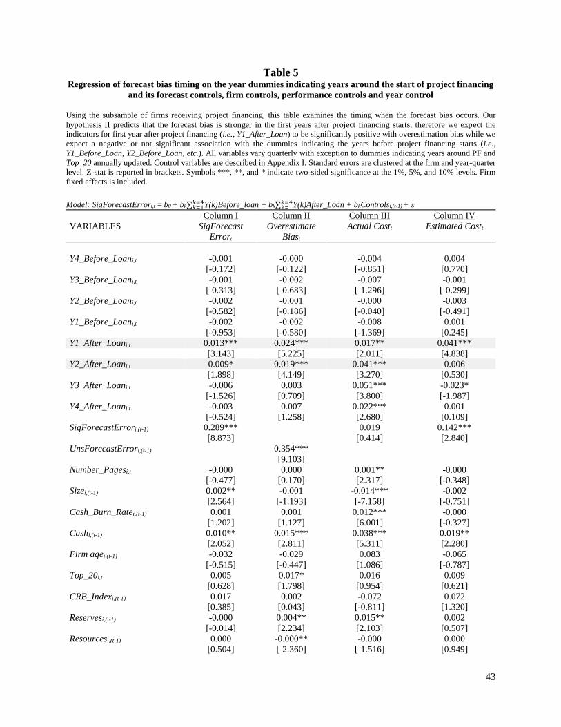
43

Table 5 Regression of forecast bias timing on the year dummies indicating years around the start of project financing

and its forecast controls, firm controls, performance controls and year control

Using the subsample of firms receiving project financing, this table examines the timing when the forecast bias occurs. Our

hypothesis II predicts that the forecast bias is stronger in the first years after project financing starts, therefore we expect the

indicators for first year after project financing (i.e., Y1_After_Loan) to be significantly positive with overestimation bias while we

expect a negative or not significant association with the dummies indicating the years before project financing starts (i.e.,

Y1_Before_Loan, Y2_Before_Loan, etc.). All variables vary quarterly with exception to dummies indicating years around PF and

Top_20 annually updated. Control variables are described in Appendix I. Standard errors are clustered at the firm and year-quarter

level. Z-stat is reported in brackets. Symbols ***, **, and * indicate two-sided significance at the 1%, 5%, and 10% levels. Firm

fixed effects is included.

Model: SigForecastErrori,t = b0 + bk∑𝑘=1

𝑘=4Y(k)Before_loan + bk∑𝑘=1𝑘=4Y(k)After_Loan + bkControlsi,(t-1) + ε


VARIABLES SigForecast

Errort

Overestimate

Biast

Actual Costt Estimated Costt

Y4_Before_Loani,t -0.001 -0.000 -0.004 0.004

[-0.172] [-0.122] [-0.851] [0.770]

Y3_Before_Loani,t -0.001 -0.002 -0.007 -0.001

[-0.313] [-0.683] [-1.296] [-0.299]

Y2_Before_Loani,t -0.002 -0.001 -0.000 -0.003

[-0.582] [-0.186] [-0.040] [-0.491]

Y1_Before_Loani,t -0.002 -0.002 -0.008 0.001

[-0.953] [-0.580] [-1.369] [0.245]

Y1_After_Loani,t 0.013*** 0.024*** 0.017** 0.041***

[3.143] [5.225] [2.011] [4.838]

Y2_After_Loani,t 0.009* 0.019*** 0.041*** 0.006

[1.898] [4.149] [3.270] [0.530]

Y3_After_Loani,t -0.006 0.003 0.051*** -0.023*

[-1.526] [0.709] [3.800] [-1.987]

Y4_After_Loani,t -0.003 0.007 0.022*** 0.001

[-0.524] [1.258] [2.680] [0.109]

SigForecastErrori,(t-1) 0.289*** 0.019 0.142***

[8.873] [0.414] [2.840]

UnsForecastErrori,(t-1) 0.354***

[9.103]

Number_Pagesi,t -0.000 0.000 0.001** -0.000

[-0.477] [0.170] [2.317] [-0.348]

Sizei,(t-1) 0.002** -0.001 -0.014*** -0.002

[2.564] [-1.193] [-7.158] [-0.751]

Cash_Burn_Ratei,(t-1) 0.001 0.001 0.012*** -0.000

[1.202] [1.127] [6.001] [-0.327]

Cashi,(t-1) 0.010** 0.015*** 0.038*** 0.019**

[2.052] [2.811] [5.311] [2.280]

Firm agei,(t-1) -0.032 -0.029 0.083 -0.065

[-0.515] [-0.447] [1.086] [-0.787]

Top_20i,t 0.005 0.017* 0.016 0.009

[0.628] [1.798] [0.954] [0.621]

CRB_Indexi,(t-1) 0.017 0.002 -0.072 0.072

[0.385] [0.043] [-0.811] [1.320]

Reservesi,(t-1) -0.000 0.004** 0.015** 0.002

[-0.014] [2.234] [2.103] [0.507]

Resourcesi,(t-1) 0.000 -0.000** -0.000 0.000

[0.504] [-2.360] [-1.516] [0.949]

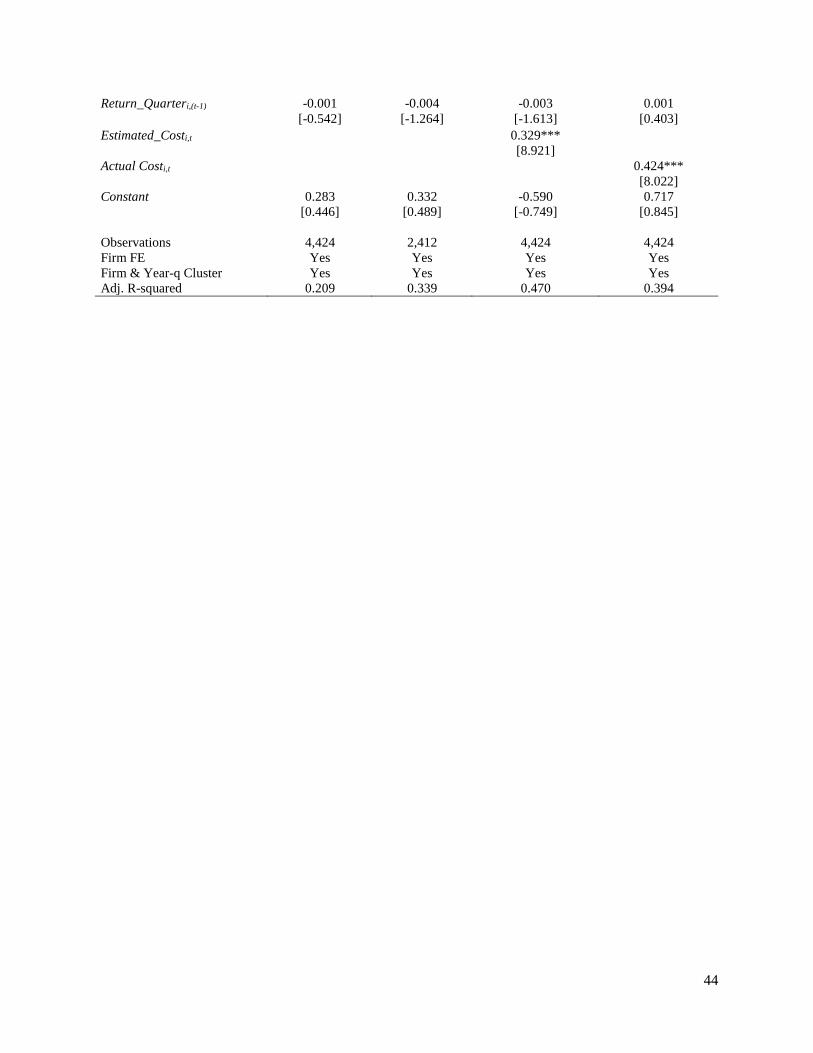
44

Return_Quarteri,(t-1) -0.001 -0.004 -0.003 0.001

[-0.542] [-1.264] [-1.613] [0.403]

Estimated_Costi,t 0.329***

[8.921]

Actual Costi,t 0.424***

[8.022]

Constant 0.283 0.332 -0.590 0.717

[0.446] [0.489] [-0.749] [0.845]

Observations 4,424 2,412 4,424 4,424

Firm FE Yes Yes Yes Yes


Adj. R-squared 0.209 0.339 0.470 0.394

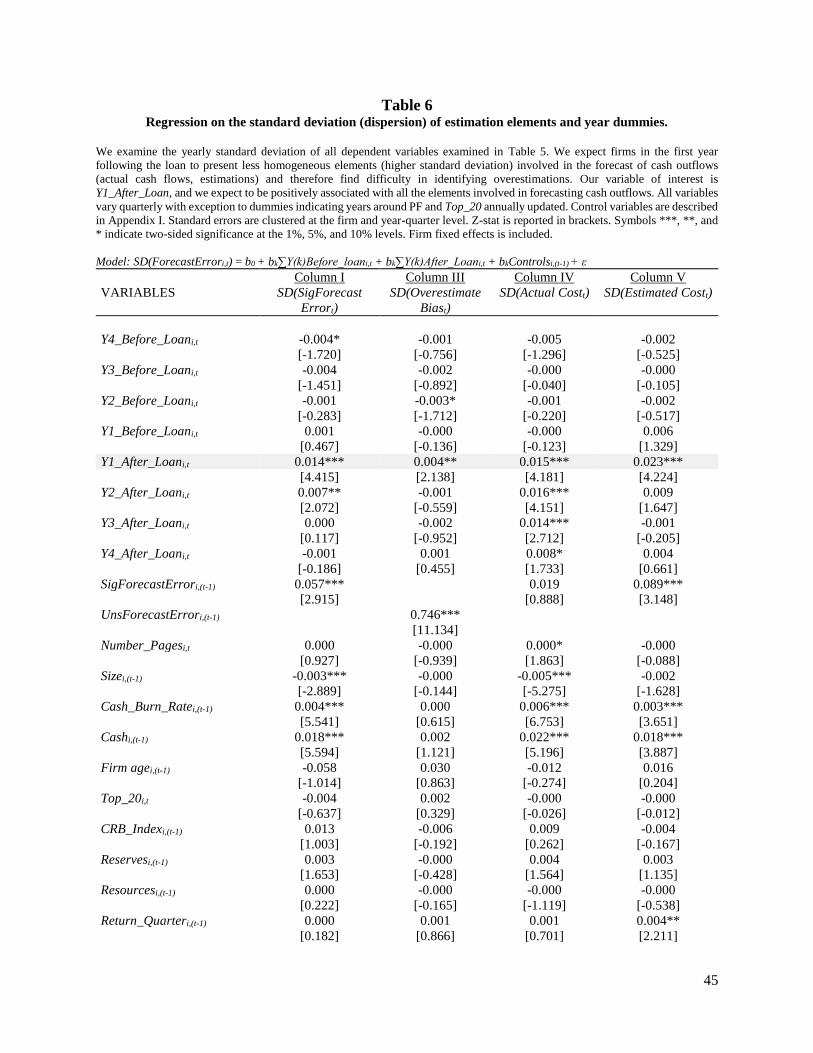
45

Table 6 Regression on the standard deviation (dispersion) of estimation elements and year dummies.

We examine the yearly standard deviation of all dependent variables examined in Table 5. We expect firms in the first year

following the loan to present less homogeneous elements (higher standard deviation) involved in the forecast of cash outflows

(actual cash flows, estimations) and therefore find difficulty in identifying overestimations. Our variable of interest is

Y1_After_Loan, and we expect to be positively associated with all the elements involved in forecasting cash outflows. All variables

vary quarterly with exception to dummies indicating years around PF and Top_20 annually updated. Control variables are described

in Appendix I. Standard errors are clustered at the firm and year-quarter level. Z-stat is reported in brackets. Symbols ***, **, and

* indicate two-sided significance at the 1%, 5%, and 10% levels. Firm fixed effects is included.

Model: SD(ForecastErrori,t) = b0 + bk∑Y(k)Before_loani,t + bk∑Y(k)After_Loani,t + bkControlsi,(t-1) + ε

Column I Column III Column IV Column V

VARIABLES SD(SigForecast

Errort)

SD(Overestimate

Biast)

SD(Actual Costt) SD(Estimated Costt)

Y4_Before_Loani,t -0.004* -0.001 -0.005 -0.002

[-1.720] [-0.756] [-1.296] [-0.525]

Y3_Before_Loani,t -0.004 -0.002 -0.000 -0.000

[-1.451] [-0.892] [-0.040] [-0.105]

Y2_Before_Loani,t -0.001 -0.003* -0.001 -0.002

[-0.283] [-1.712] [-0.220] [-0.517]

Y1_Before_Loani,t 0.001 -0.000 -0.000 0.006

[0.467] [-0.136] [-0.123] [1.329]

Y1_After_Loani,t 0.014*** 0.004** 0.015*** 0.023***

[4.415] [2.138] [4.181] [4.224]

Y2_After_Loani,t 0.007** -0.001 0.016*** 0.009

[2.072] [-0.559] [4.151] [1.647]

Y3_After_Loani,t 0.000 -0.002 0.014*** -0.001

[0.117] [-0.952] [2.712] [-0.205]

Y4_After_Loani,t -0.001 0.001 0.008* 0.004

[-0.186] [0.455] [1.733] [0.661]

SigForecastErrori,(t-1) 0.057*** 0.019 0.089***

[2.915] [0.888] [3.148]

UnsForecastErrori,(t-1) 0.746***

[11.134]

Number_Pagesi,t 0.000 -0.000 0.000* -0.000

[0.927] [-0.939] [1.863] [-0.088]

Sizei,(t-1) -0.003*** -0.000 -0.005*** -0.002

[-2.889] [-0.144] [-5.275] [-1.628]

Cash_Burn_Ratei,(t-1) 0.004*** 0.000 0.006*** 0.003***

[5.541] [0.615] [6.753] [3.651]

Cashi,(t-1) 0.018*** 0.002 0.022*** 0.018***

[5.594] [1.121] [5.196] [3.887]

Firm agei,(t-1) -0.058 0.030 -0.012 0.016

[-1.014] [0.863] [-0.274] [0.204]

Top_20i,t -0.004 0.002 -0.000 -0.000

[-0.637] [0.329] [-0.026] [-0.012]

CRB_Indexi,(t-1) 0.013 -0.006 0.009 -0.004

[1.003] [-0.192] [0.262] [-0.167]

Reservesi,(t-1) 0.003 -0.000 0.004 0.003

[1.653] [-0.428] [1.564] [1.135]

Resourcesi,(t-1) 0.000 -0.000 -0.000 -0.000

[0.222] [-0.165] [-1.119] [-0.538]

Return_Quarteri,(t-1) 0.000 0.001 0.001 0.004**

[0.182] [0.866] [0.701] [2.211]

46

Constant 0.659 -0.304 0.237 -0.108

[1.124] [-0.847] [0.505] [-0.134]

Observations 4,365 2,882 4,368 4,368



Adj. R-squared 0.316 0.622 0.349 0.293

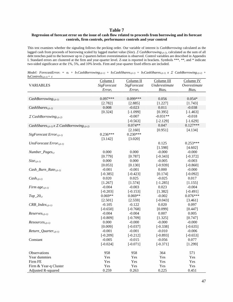
47

Table 7 Regression of forecast error on the issue of cash flow related to proceeds from borrowing and its forecast

controls, firm controls, performance controls and year control

This test examines whether the signaling follows the pecking order. Our variable of interest is CashBorrowing calculated as the

lagged cash from proceeds of borrowing scaled by lagged market value (Size). CashBorrowingi,(t-2), calculated as the sum of all

debt trenches paid to the borrower up to 2 quarters before overestimation is observed. Control variables are described in Appendix

I. Standard errors are clustered at the firm and year-quarter level. Z-stat is reported in brackets. Symbols ***, **, and * indicate

two-sided significance at the 1%, 5%, and 10% levels. Firm and year-quarter fixed effects are included.

Model: ForecastErrort = αt + b1CashBorrowingi,(t-1) + b2CashSharesi,(t-1) + b3CashSharesi,(t-1) x CashBorrowingi,(t-2) +

bkControlsi,(t-1) + ε


VARIABLES SigForecast

Errort

SigForecast

Errort

Underestimate

Biast

Overestimate

Biast

CashBorrowingi,(t-1) 0.097*** 0.099*** 0.056 0.054*

[2.782] [2.885] [1.227] [1.743]

CashSharesi,(t-1) 0.008 -0.023 0.011 -0.038

[0.324] [-1.099] [0.395] [-1.463]

CashBorrowingi,(t-2) -0.007 -0.031** -0.018

[-0.563] [-2.129] [-1.629]

CashSharesi,(t-1) x CashBorrowingi,(t-2) 0.074** 0.047 0.127***

[2.160] [0.951] [4.134]

SigForecast Errort,(t-1) 0.236*** 0.230***

[3.142] [3.020]

UnsForecast Errort,(t-1) 0.125 0.253***

[1.598] [4.602]

Number_Pagesi,t 0.000 0.000 -0.000 -0.000

[0.779] [0.787] [-0.343] [-0.372]

Sizei,(t-1) 0.000 0.000 -0.005 -0.003

[0.053] [0.130] [-0.939] [-0.860]

Cash_Burn_Ratei,(t-1) -0.001 -0.001 0.000 -0.000

[-0.385] [-0.423] [0.174] [-0.092]

Cashi,(t-1) 0.020 0.025 -0.025 0.017

[1.267] [1.574] [-1.285] [1.155]

Firm agei,(t-1) -0.004 -0.003 0.023 -0.004

[-0.203] [-0.153] [1.382] [-0.491]

Top_20i,t 0.069** 0.069** -0.002 0.076***

[2.501] [2.559] [-0.043] [3.461]

CRB_Indexi,(t-1) -0.105 -0.122 0.020 0.097

[-0.650] [-0.768] [0.099] [0.447]

Reservesi,(t-1) -0.004 -0.004 0.007 0.005

[-0.809] [-0.709] [1.325] [0.747]

Resourcesi,(t-1) 0.000 -0.000 -0.000 -0.000

[0.009] [-0.037] [-0.338] [-0.635]

Return_Quarteri,(t-1) -0.001 -0.001 -0.010 -0.006

[-0.209] [-0.212] [-0.893] [-0.653]

Constant -0.005 -0.015 -0.056 0.077

[-0.024] [-0.071] [-0.371] [1.299]

Observations 958 958 364 571

Year dummies Yes Yes Yes Yes



Adjusted R-squared 0.259 0.263 0.225 0.451

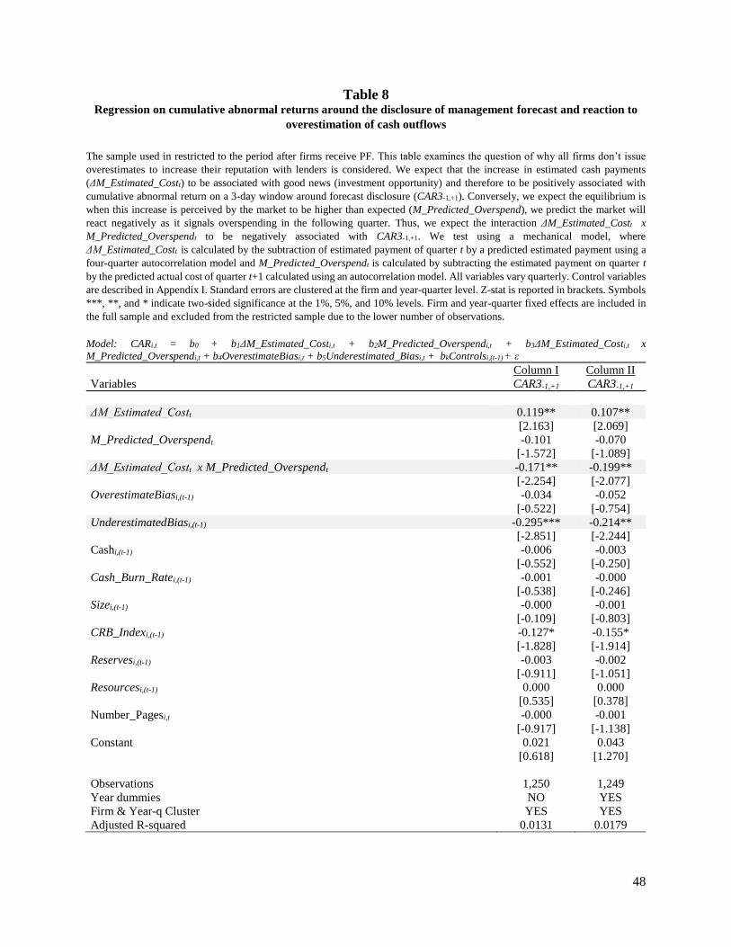
48

Table 8 Regression on cumulative abnormal returns around the disclosure of management forecast and reaction to

overestimation of cash outflows

The sample used in restricted to the period after firms receive PF. This table examines the question of why all firms don’t issue

overestimates to increase their reputation with lenders is considered. We expect that the increase in estimated cash payments

(ΔM_Estimated_Costt) to be associated with good news (investment opportunity) and therefore to be positively associated with

cumulative abnormal return on a 3-day window around forecast disclosure (CAR3-1,+1). Conversely, we expect the equilibrium is

when this increase is perceived by the market to be higher than expected (M_Predicted_Overspend), we predict the market will

react negatively as it signals overspending in the following quarter. Thus, we expect the interaction ΔM_Estimated_Costt x

M_Predicted_Overspendt to be negatively associated with CAR3-1,+1. We test using a mechanical model, where

ΔM_Estimated_Costt is calculated by the subtraction of estimated payment of quarter t by a predicted estimated payment using a

four-quarter autocorrelation model and M_Predicted_Overspendt is calculated by subtracting the estimated payment on quarter t

by the predicted actual cost of quarter t+1 calculated using an autocorrelation model. All variables vary quarterly. Control variables

are described in Appendix I. Standard errors are clustered at the firm and year-quarter level. Z-stat is reported in brackets. Symbols

***, **, and * indicate two-sided significance at the 1%, 5%, and 10% levels. Firm and year-quarter fixed effects are included in

the full sample and excluded from the restricted sample due to the lower number of observations.

Model: CARi,t = b0 + b1ΔM_Estimated_Costi,t + b2M_Predicted_Overspendi,t + b3ΔM_Estimated_Costi,t x

M_Predicted_Overspendi,t + b4OverestimateBiasi,t + b5Underestimated_Biasi,t + bkControlsi,(t-1) + ε

Column I Column II

Variables CAR3-1,+1 CAR3-1,+1

ΔM_Estimated_Costt 0.119** 0.107**

[2.163] [2.069]

M_Predicted_Overspendt -0.101 -0.070

[-1.572] [-1.089]

ΔM_Estimated_Costt x M_Predicted_Overspendt -0.171** -0.199**

[-2.254] [-2.077]

OverestimateBiasi,(t-1) -0.034 -0.052

[-0.522] [-0.754]

UnderestimatedBiasi,(t-1) -0.295*** -0.214**

[-2.851] [-2.244]

Cashi,(t-1) -0.006 -0.003

[-0.552] [-0.250]

Cash_Burn_Ratei,(t-1) -0.001 -0.000

[-0.538] [-0.246]

Sizei,(t-1) -0.000 -0.001

[-0.109] [-0.803]

CRB_Indexi,(t-1) -0.127* -0.155*

[-1.828] [-1.914]

Reservesi,(t-1) -0.003 -0.002

[-0.911] [-1.051]

Resourcesi,(t-1) 0.000 0.000

[0.535] [0.378]

Number_Pagesi,t -0.000 -0.001

[-0.917] [-1.138]

Constant 0.021 0.043

[0.618] [1.270]

Observations 1,250 1,249

Year dummies NO YES

Firm & Year-q Cluster YES YES

Adjusted R-squared 0.0131 0.0179

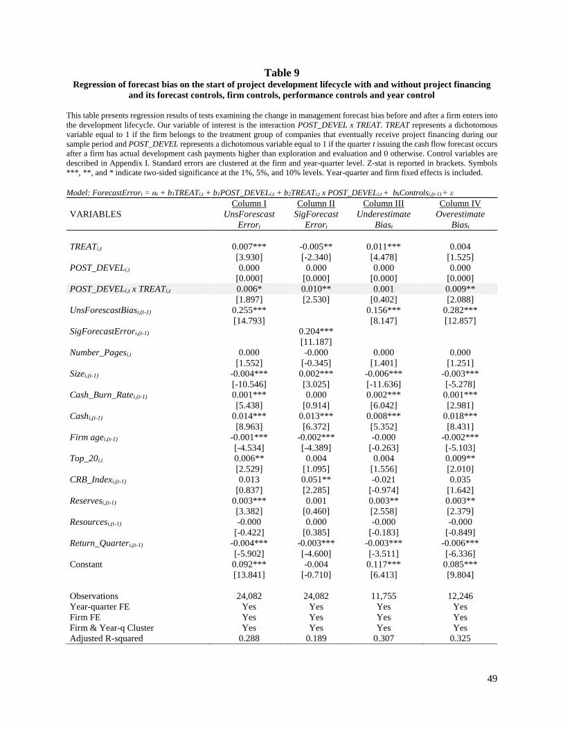
49

Table 9 Regression of forecast bias on the start of project development lifecycle with and without project financing

and its forecast controls, firm controls, performance controls and year control

This table presents regression results of tests examining the change in management forecast bias before and after a firm enters into

the development lifecycle. Our variable of interest is the interaction POST_DEVEL x TREAT. TREAT represents a dichotomous

variable equal to 1 if the firm belongs to the treatment group of companies that eventually receive project financing during our

sample period and POST_DEVEL represents a dichotomous variable equal to 1 if the quarter t issuing the cash flow forecast occurs

after a firm has actual development cash payments higher than exploration and evaluation and 0 otherwise. Control variables are

described in Appendix I. Standard errors are clustered at the firm and year-quarter level. Z-stat is reported in brackets. Symbols

***, **, and * indicate two-sided significance at the 1%, 5%, and 10% levels. Year-quarter and firm fixed effects is included.

Model: ForecastErrort = αt + b1TREATi,t + b1POST_DEVELi,t + b2TREATi,t x POST_DEVELi,t + bkControlsi,(t-1) + ε



Errort

SigForecast

Errort

Underestimate

Biast

Overestimate

Biast

TREATi,t 0.007*** -0.005** 0.011*** 0.004

[3.930] [-2.340] [4.478] [1.525]

POST_DEVELi,t 0.000 0.000 0.000 0.000

[0.000] [0.000] [0.000] [0.000]

POST_DEVELi,t x TREATi,t 0.006* 0.010** 0.001 0.009**

[1.897] [2.530] [0.402] [2.088]

UnsForescastBiasi,(t-1) 0.255*** 0.156*** 0.282***

[14.793] [8.147] [12.857]


[11.187]

Number_Pagesi,t 0.000 -0.000 0.000 0.000

[1.552] [-0.345] [1.401] [1.251]

Sizei,(t-1) -0.004*** 0.002*** -0.006*** -0.003***

[-10.546] [3.025] [-11.636] [-5.278]

Cash_Burn_Ratei,(t-1) 0.001*** 0.000 0.002*** 0.001***

[5.438] [0.914] [6.042] [2.981]

Cashi,(t-1) 0.014*** 0.013*** 0.008*** 0.018***

[8.963] [6.372] [5.352] [8.431]

Firm agei,(t-1) -0.001*** -0.002*** -0.000 -0.002***

[-4.534] [-4.389] [-0.263] [-5.103]

Top_20i,t 0.006** 0.004 0.004 0.009**

[2.529] [1.095] [1.556] [2.010]

CRB_Indexi,(t-1) 0.013 0.051** -0.021 0.035

[0.837] [2.285] [-0.974] [1.642]

Reservesi,(t-1) 0.003*** 0.001 0.003** 0.003**

[3.382] [0.460] [2.558] [2.379]

Resourcesi,(t-1) -0.000 0.000 -0.000 -0.000

[-0.422] [0.385] [-0.183] [-0.849]

Return_Quarteri,(t-1) -0.004*** -0.003*** -0.003*** -0.006***

[-5.902] [-4.600] [-3.511] [-6.336]

Constant 0.092*** -0.004 0.117*** 0.085***

[13.841] [-0.710] [6.413] [9.804]

Observations 24,082 24,082 11,755 12,246





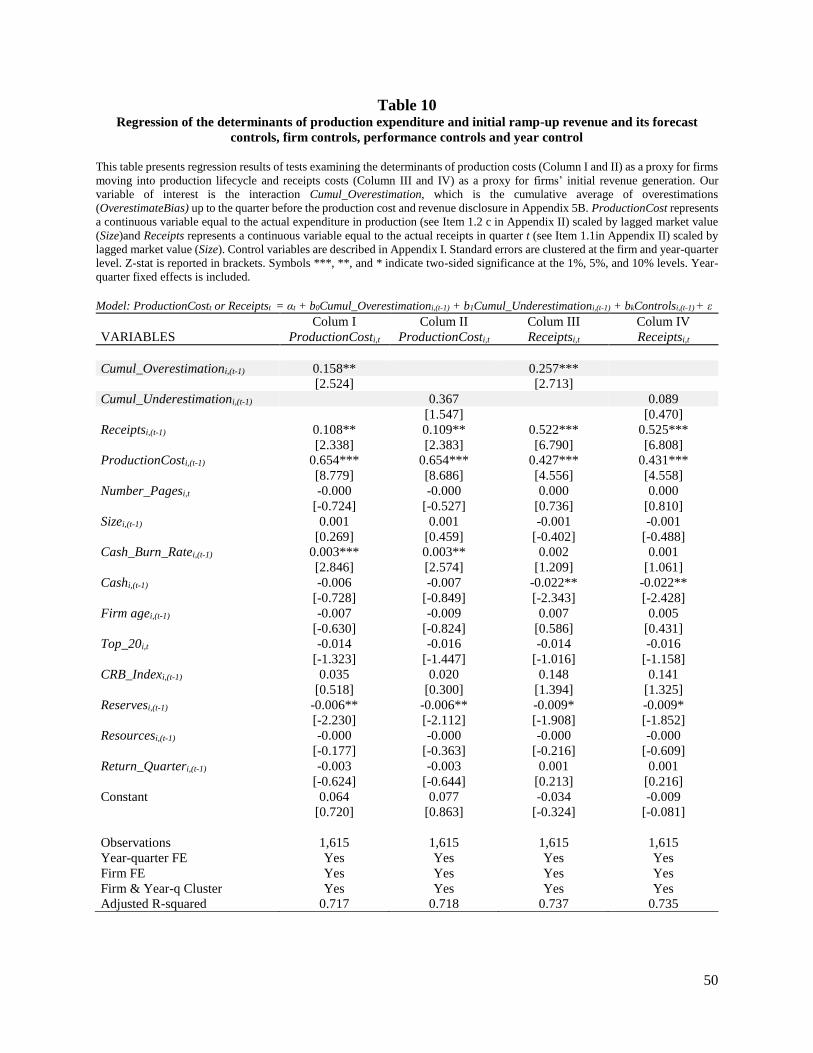
50

Table 10 Regression of the determinants of production expenditure and initial ramp-up revenue and its forecast

controls, firm controls, performance controls and year control

This table presents regression results of tests examining the determinants of production costs (Column I and II) as a proxy for firms

moving into production lifecycle and receipts costs (Column III and IV) as a proxy for firms’ initial revenue generation. Our

variable of interest is the interaction Cumul_Overestimation, which is the cumulative average of overestimations

(OverestimateBias) up to the quarter before the production cost and revenue disclosure in Appendix 5B. ProductionCost represents

a continuous variable equal to the actual expenditure in production (see Item 1.2 c in Appendix II) scaled by lagged market value

(Size)and Receipts represents a continuous variable equal to the actual receipts in quarter t (see Item 1.1in Appendix II) scaled by

lagged market value (Size). Control variables are described in Appendix I. Standard errors are clustered at the firm and year-quarter

level. Z-stat is reported in brackets. Symbols ***, **, and * indicate two-sided significance at the 1%, 5%, and 10% levels. Year-

quarter fixed effects is included.

Model: ProductionCostt or Receiptst = αt + b0Cumul_Overestimationi,(t-1) + b1Cumul_Underestimationi,(t-1) + bkControlsi,(t-1) + ε

Colum I Colum II Colum III Colum IV

VARIABLES ProductionCosti,t ProductionCosti,t Receiptsi,t Receiptsi,t

Cumul_Overestimationi,(t-1) 0.158** 0.257***

[2.524] [2.713]

Cumul_Underestimationi,(t-1) 0.367 0.089

[1.547] [0.470]

Receiptsi,(t-1) 0.108** 0.109** 0.522*** 0.525***

[2.338] [2.383] [6.790] [6.808]

ProductionCosti,(t-1) 0.654*** 0.654*** 0.427*** 0.431***

[8.779] [8.686] [4.556] [4.558]

Number_Pagesi,t -0.000 -0.000 0.000 0.000

[-0.724] [-0.527] [0.736] [0.810]

Sizei,(t-1) 0.001 0.001 -0.001 -0.001

[0.269] [0.459] [-0.402] [-0.488]

Cash_Burn_Ratei,(t-1) 0.003*** 0.003** 0.002 0.001

[2.846] [2.574] [1.209] [1.061]

Cashi,(t-1) -0.006 -0.007 -0.022** -0.022**

[-0.728] [-0.849] [-2.343] [-2.428]

Firm agei,(t-1) -0.007 -0.009 0.007 0.005

[-0.630] [-0.824] [0.586] [0.431]

Top_20i,t -0.014 -0.016 -0.014 -0.016

[-1.323] [-1.447] [-1.016] [-1.158]

CRB_Indexi,(t-1) 0.035 0.020 0.148 0.141

[0.518] [0.300] [1.394] [1.325]

Reservesi,(t-1) -0.006** -0.006** -0.009* -0.009*

[-2.230] [-2.112] [-1.908] [-1.852]

Resourcesi,(t-1) -0.000 -0.000 -0.000 -0.000

[-0.177] [-0.363] [-0.216] [-0.609]

Return_Quarteri,(t-1) -0.003 -0.003 0.001 0.001

[-0.624] [-0.644] [0.213] [0.216]

Constant 0.064 0.077 -0.034 -0.009

[0.720] [0.863] [-0.324] [-0.081]

Observations 1,615 1,615 1,615 1,615





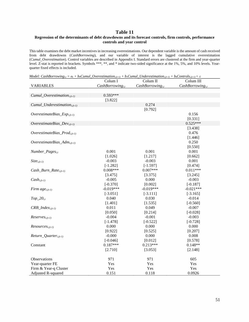
51

Table 11 Regression of the determinants of debt drawdowns and its forecast controls, firm controls, performance

controls and year control

This table examines the debt market incentives in increasing overestimations. Our dependent variable is the amount of cash received

from debt drawdowns (CashBorrowing), and our variable of interest is the lagged cumulative overestimation

(Cumul_Overestimation). Control variables are described in Appendix I. Standard errors are clustered at the firm and year-quarter

level. Z-stat is reported in brackets. Symbols ***, **, and * indicate two-sided significance at the 1%, 5%, and 10% levels. Year-

quarter fixed effects is included.

Model: CashBorrowingi,t = αt + b0Cumul_Overestimationi,(t-1) + b1Cumul_Underestimationi,(t-1) + bkControlsi,(t-1) + ε

Colum I Colum II Colum III

VARIABLES CashBorrowingi,t CashBorrowingi,t CashBorrowingi,t

Cumul_Overestimationi,(t-1) 0.593***

[3.822]

Cumul_Underestimationi,(t-1) 0.274

[0.792]

OverestimateBias_Expi,(t-1) 0.156

[0.331]

OverestimateBias_Devi,(t-1) 0.525***

[3.438]

OverestimateBias_Prodi,(t-1) 0.476

[1.446]

OverestimateBias_Admi,(t-1) 0.250

[0.550]

Number_Pagesi,t 0.001 0.001 0.001

[1.026] [1.217] [0.662]

Sizei,(t-1) -0.003 -0.003 0.001

[-1.282] [-1.597] [0.474]

Cash_Burn_Ratei,(t-1) 0.008*** 0.007*** 0.011***

[3.475] [3.375] [3.245]

Cashi,(t-1) -0.005 0.000 -0.003

[-0.370] [0.002] [-0.187]

Firm agei,(t-1) -0.019*** -0.019*** -0.021***

[-3.051] [-3.111] [-3.165]

Top_20i,t 0.040 0.030 -0.014

[1.401] [1.535] [-0.560]

CRB_Indexi,(t-1) 0.011 0.049 -0.007

[0.050] [0.214] [-0.028]

Reservesi,(t-1) -0.004 -0.001 -0.003

[-1.478] [-0.522] [-0.728]

Resourcesi,(t-1) 0.000 0.000 0.000

[0.922] [0.525] [0.207]

Return_Quarteri,(t-1) -0.000 0.000 0.008

[-0.046] [0.012] [0.578]

Constant 0.187*** 0.213*** 0.148**

[2.710] [3.053] [2.148]

Observations 971 971 605

Year-quarter FE Yes Yes Yes

Firm & Year-q Cluster Yes Yes Yes

Adjusted R-squared 0.151 0.118 0.0926

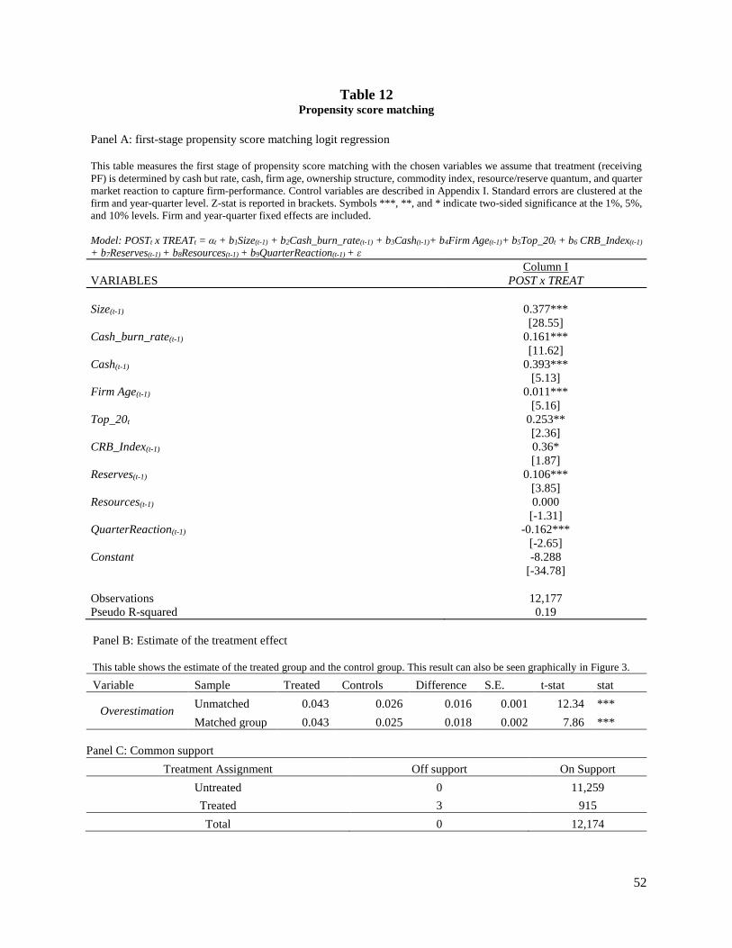
52

Table 12 Propensity score matching

Panel A: first-stage propensity score matching logit regression

This table measures the first stage of propensity score matching with the chosen variables we assume that treatment (receiving

PF) is determined by cash but rate, cash, firm age, ownership structure, commodity index, resource/reserve quantum, and quarter

market reaction to capture firm-performance. Control variables are described in Appendix I. Standard errors are clustered at the

firm and year-quarter level. Z-stat is reported in brackets. Symbols ***, **, and * indicate two-sided significance at the 1%, 5%,

and 10% levels. Firm and year-quarter fixed effects are included.

Model: POSTt x TREATt = αt + b1Size(t-1) + b2Cash_burn_rate(t-1) + b3Cash(t-1)+ b4Firm Age(t-1)+ b5Top_20t + b6 CRB_Index(t-1)

+ b7Reserves(t-1) + b8Resources(t-1) + b9QuarterReaction(t-1) + ε Column I

VARIABLES POST x TREAT

Size(t-1) 0.377***

[28.55]

Cash_burn_rate(t-1) 0.161***

[11.62]

Cash(t-1) 0.393***

[5.13]

Firm Age(t-1) 0.011***

[5.16]

Top_20t 0.253**

[2.36]

CRB_Index(t-1) 0.36*

[1.87]

Reserves(t-1) 0.106***

[3.85]

Resources(t-1) 0.000

[-1.31]

QuarterReaction(t-1) -0.162***

[-2.65]

Constant -8.288

[-34.78]

Observations 12,177

Pseudo R-squared 0.19

Panel B: Estimate of the treatment effect

This table shows the estimate of the treated group and the control group. This result can also be seen graphically in Figure 3.

Variable Sample Treated Controls Difference S.E. t-stat stat

Overestimation Unmatched 0.043 0.026 0.016 0.001 12.34 ***

Matched group 0.043 0.025 0.018 0.002 7.86 ***

Panel C: Common support

Treatment Assignment Off support On Support

Untreated 0 11,259

Treated 3 915

Total 0 12,174

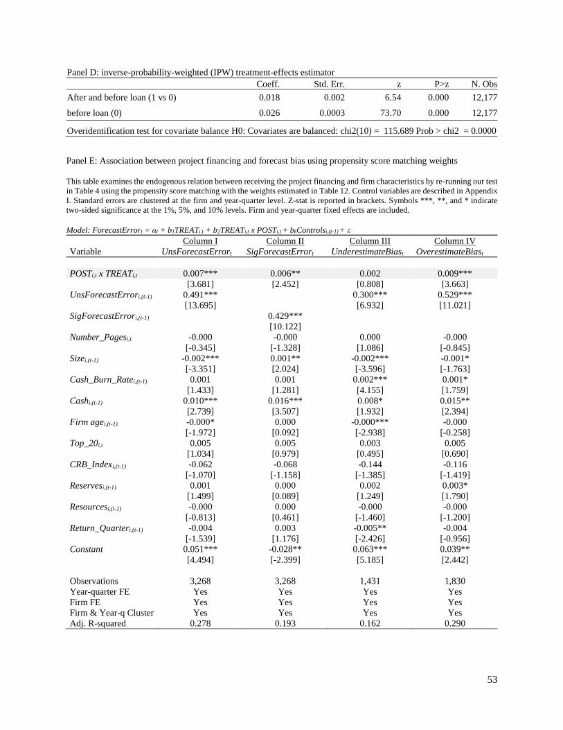
53

Panel D: inverse-probability-weighted (IPW) treatment-effects estimator

Coeff. Std. Err. z P>z N. Obs

After and before loan (1 vs 0) 0.018 0.002 6.54 0.000 12,177

before loan (0) 0.026 0.0003 73.70 0.000 12,177

Overidentification test for covariate balance H0: Covariates are balanced: chi2(10) = 115.689 Prob > chi2 = 0.0000

Panel E: Association between project financing and forecast bias using propensity score matching weights

This table examines the endogenous relation between receiving the project financing and firm characteristics by re-running our test

in Table 4 using the propensity score matching with the weights estimated in Table 12. Control variables are described in Appendix

I. Standard errors are clustered at the firm and year-quarter level. Z-stat is reported in brackets. Symbols ***, **, and * indicate

two-sided significance at the 1%, 5%, and 10% levels. Firm and year-quarter fixed effects are included.

Model: ForecastErrort = αt + b1TREATi,t + b2TREATi,t x POSTi,t + bkControlsi,(t-1) + ε


Variable UnsForecastErrort SigForecastErrort UnderestimateBiast OverestimateBiast

POSTi,t x TREATi,t 0.007*** 0.006** 0.002 0.009***

[3.681] [2.452] [0.808] [3.663]


[13.695] [6.932] [11.021]


[10.122]

Number_Pagesi,t -0.000 -0.000 0.000 -0.000

[-0.345] [-1.328] [1.086] [-0.845]

Sizei,(t-1) -0.002*** 0.001** -0.002*** -0.001*

[-3.351] [2.024] [-3.596] [-1.763]

Cash_Burn_Ratei,(t-1) 0.001 0.001 0.002*** 0.001*

[1.433] [1.281] [4.155] [1.759]

Cashi,(t-1) 0.010*** 0.016*** 0.008* 0.015**

[2.739] [3.507] [1.932] [2.394]

Firm agei,(t-1) -0.000* 0.000 -0.000*** -0.000

[-1.972] [0.092] [-2.938] [-0.258]

Top_20i,t 0.005 0.005 0.003 0.005

[1.034] [0.979] [0.495] [0.690]

CRB_Indexi,(t-1) -0.062 -0.068 -0.144 -0.116

[-1.070] [-1.158] [-1.385] [-1.419]

Reservesi,(t-1) 0.001 0.000 0.002 0.003*

[1.499] [0.089] [1.249] [1.790]

Resourcesi,(t-1) -0.000 0.000 -0.000 -0.000

[-0.813] [0.461] [-1.460] [-1.200]

Return_Quarteri,(t-1) -0.004 0.003 -0.005** -0.004

[-1.539] [1.176] [-2.426] [-0.956]

Constant 0.051*** -0.028** 0.063*** 0.039**

[4.494] [-2.399] [5.185] [2.442]

Observations 3,268 3,268 1,431 1,830




Adj. R-squared 0.278 0.193 0.162 0.290

54

Appendix I

List of Variable Definitions Dependent Variables:

SigForecastError Signed estimated payments (estimated, see example on “estimated cash payments”

on section 1.5, page 3, of Appendix II) for quarter t minus realized payments for

quarter t (Actual, see example on “actual cash flow spent” on section 1.2, page 1, of

Appendix II), deflated by lagged market value (Size). This variable is composed of

four different types of mandatory forecasts of payment along with current period

actuals. These four forecasts include management forecasts of exploration and

evaluation expenditure, management forecasts of development expenditure,

management forecasts of production expenditure, and management forecasts of

administration expenditure (see 5B example in Appendix II). The cash flow

payments are for operating activities and only represent cash outflows as the firms

don’t have relevant sales given their pre-production status.

UnsForecastError Absolute value of SigForecastError.

OverestimateBias The unsigned Bias when SigForecastError > 0. This unsigned variable captures the

overestimation of cash flow payments (expected payments higher than actual). Also

associated with budget slack or underspending.

UnderestimateBias The unsigned Bias when SigForecastError <= 0. This unsigned variable captures

the underestimation of cash flow payments (expected payments lower than actual).

It is also associated with cost (budget) overruns or overspending.

Estimated_Cost Estimated value of cash flow of operations on quarter t scaled by lagged size

(estimated, see an example on “estimated cash payments” on section 1.5, page 3, of

Appendix II).

Actual_Cost Actual value of cash outflow of operations on quarter t scaled by lagged size

(Actual, see example on “actual cash flow spent” on section 1.2, page 1, of

Appendix II).

CAR3(-1,+1) 3-day Cumulative abnormal return around the forecast disclosure.

ProductionCost Continuous variable equal to the actual expenditure in production (see Item 1.2 c in

Appendix II) scaled by lagged market value (Size).

Receipts Continuous variable equal to the actual revenue in quarter t (see Item 1.1in

Appendix II) scaled by lagged market value (Size).

Explanatory Variable:

TREAT A dichotomous variable equal to 1 if the firm belongs to the treatment group of

MEE companies that eventually receive project financing during our sample period

and 0 otherwise. We consider in this group firms receiving the seed, bridge, and

first tranche of project financing.

POST x TREAT A dichotomous variable equal to 1 if the quarter t issuing the cash flow forecast

occurs after receiving a project financing loan and 0 otherwise. The interaction

POST x TREAT test allows us to examine if the overall forecast precision changes

after receiving TREAT and controls for the group difference between firms

receiving project financing and those that do not.

55

Y4_Before_Loan,

Y3_Before_Loan,

Y2_Before_Loan and

Y1_Before_Loan

Dichotomous variables indicating each one of the five years before the loan.

Y1_After_Loan,

Y2_After_Loan, Y3_After_Loan

and Y4_After_Loan

Dichotomous variables indicating each one of the five years after the loan.

CashBorrowing Calculated by cash inflow from borrowing (Item 1.18 from Appendix 5B) scaled by

lagged market value (Size).

CashShares Calculated by cash inflow from proceeds from issues of shares (Item 1.16 from

Appendix 5B) scaled by lagged market value (Size).

ΔEstimated_Cost Calculated by subtracting the estimated payment in quarter t by estimated payment

in quarter t-1 (naïve model) scaled by lagged market value (Size).

Predicted_Overspend Calculated by subtracting estimated payment for quarter t+1 by actual payment on

quarter t (naïve model) scaled by lagged market value (Size).

ΔM_Estimated_Cost Mechanical model calculated by the subtraction of estimated payment of quarter t

by a predicted estimated payment using a four-quarter autocorrelation model.

M_Predicted_Overspend Mechanical model calculated by subtracting the estimated payment on quarter t by

the predicted actual cost of quarter t+1 calculated using an autocorrelation model.

Cumul_Overestimation Cumulative average of OverestimateBias.

Cumul_Underestimation Cumulative average of UnderestimateBias.

Control Variables:

Number_Pages Number of pages in each report

Size Disclosing firm’s size measured by 60-days average market capitalization lagged

two months before the announcement (Kato et al. (2009)).

Cash_Burn_Rate Quarterly cash burn rate variable calculated as the multiplicative inverse of the cash

at the end of the month divided by the cash outflow as the sum of the actual cash

outflows with Exploration and Evaluation, Development, Production and

Administration.

Cash Cash at the end of the quarter scaled by Size.

Return on Assets Return on assets calculated as the net income divided by total assets.

Leverage Proportion of total debt scaled by shareholder’s equity.

Firm age The number of years the firm has been listed up to the day of the announcement.

56

Top_20 Fraction of shares owned by the 20 largest owners.

CRB_Index CRB (Commodity Research Bureau) index return between 10 days before the report

and 6-months before the report.

Reserves Amount of reserves in the quarter before the forecast quarter scaled by Size.

Resources Amount of resources in the quarter before the forecast quarter scaled by Size.

Return_Quarter Buy-and-hold return in the quarter before the forecast.

Loan_Amount_TA Total amount provided by the PF scaled by total assets from the year before the loan

is provided.

Loan_Amount_SE Total amount provided by the PF scaled by shareholder’s equity from the year

before the loan is provided.

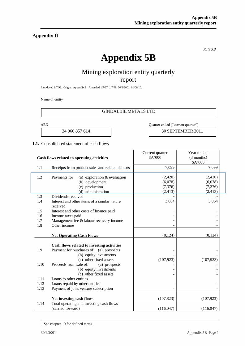
Appendix 5B

Mining exploration entity quarterly report

+ See chapter 19 for defined terms.

30/9/2001 Appendix 5B Page 1

Appendix II

Appendix 5B

Mining exploration entity quarterly

report Introduced 1/7/96. Origin: Appendix 8. Amended 1/7/97, 1/7/98, 30/9/2001, 01/06/10.

Name of entity

Rule 5.3

ABN Quarter ended (“current quarter”)

1.1. Consolidated statement of cash flows

Cash flows related to operating activities

1.1 Receipts from product sales and related debtors

1.2 Payments for (a) exploration & evaluation

(b) development

(c) production

(d) administration

1.3 Dividends received

1.4 Interest and other items of a similar nature

received

1.5 Interest and other costs of finance paid

1.6 Income taxes paid

1.7 Management fee & labour recovery income

1.8 Other income

Net Operating Cash Flows

Current quarter

$A’000

Year to date

(3 months)

$A’000

7,099

(2,420)

(6,078)

(7,376)

(2,413)

-

3,064

-

-

-

-

7,099

(2,420)

(6,078)

(7,376)

(2,413)

-

3,064

-

-

-

-

(8,124)

(8,124)

Cash flows related to investing activities 1.9 Payment for purchases of: (a) prospects

(b) equity investments

(c) other fixed assets

1.10 Proceeds from sale of: (a) prospects

(b) equity investments

(c) other fixed assets

1.11 Loans to other entities

1.12 Loans repaid by other entities

1.13 Payment of joint venture subscription

Net investing cash flows

1.14 Total operating and investing cash flows

(carried forward)

-

-

(107,923)

-

-

-

-

-

-

-

(107,923)

-

-

-

-

-

(107,823)

(107,923)

(116,047)

(116,047)

GINDALBIE METALS LTD

24 060 857 614 30 SEPTEMBER 2011

Appendix 5B




1.15 Total operating and investing cash flows

(brought forward)

(116,047) (116,047)

Cash flows related to financing activities

133,966

133,966 1.16 Proceeds from issues of shares, options, etc.

1.17 Proceeds from sale of forfeited shares - -

1.18 Proceeds from borrowings 135,319 135,319

1.19 Repayment of borrowings - -

1.20 Dividends paid - -

1.21 Capital raising costs (3,929) (3,929)

1.22 Payments for cash backing of performance (8,569) (8,569)

bonds

Net financing cash flows

256,787

256,787

Net increase (decrease) in cash held

140,740

140,740

1.23 Cash at beginning of quarter/year to date 236,633 236,633

1.24 Exchange rate adjustments to item 1.23

1.25 Cash at end of quarter

377,373

377,373

1.2. Payments to directors of the entity and associates of the directors

Payments to related entities of the entity and associates of the related entities

1.28 Explanation necessary for an understanding of the transactions

Directors remuneration 1,147

1.3. Non-cash financing and investing activities

2.1 Details of financing and investing transactions which have had a material effect on consolidated

assets and liabilities but did not involve cash flows

2.2 Details of outlays made by other entities to establish or increase their share in projects in which the

reporting entity has an interest

Current quarter

$A'000

1,147

1.26 Aggregate amount of payments to the parties included in item 1.2

1.27 Aggregate amount of loans to the parties included in item 1.11

Appendix 5B




1.4. Financing facilities available

Add notes as necessary for an understanding of the position.

3.1 Loan facilities

3.2 Credit standby arrangements

1.5. Estimated cash outflows for next quarter

4.1 Exploration and evaluation

4.2 Development

4.3 Production

4.4 Administration

$A’000

9,818

3,195

9,799

1,917

Total

24,729

Reconciliation of cash

Reconciliation of cash at the end of the quarter (as

shown in the consolidated statement of cash flows) to

the related items in the accounts is as follows.

Current quarter

$A’000

Previous quarter

$A’000

5.1 Cash on hand and at bank

5.2 Deposits at call

5.3 Bank overdraft

5.4 Other (provide details)

148,547 91,454

228,826 145,179

- -

- -

Total: cash at end of quarter (item 1.25) 377,373 236,633

1.6. Changes in interests in mining tenements

6.1 Interests in mining

tenements relinquished,

reduced or lapsed

6.2 Interests in mining

tenements acquired or

increased

Amount available

$A’000

Amount used

$A’000

71,075 544,579

- -

Tenement

reference

Nature of interest

(note (2))

Interest at

beginning

of quarter

Interest at

end of

quarter

Appendix 5B




1.7. Issued and quoted securities at end of current quarter

Description includes rate of interest and any redemption or conversion rights together with prices and dates.

Total number Number

quoted

Issue price per

security (see note 3)

(cents)

Amount paid up per

security (see note 3)

(cents)

7.1 Preference +securities (description)

7.2 Changes during

quarter

(a) Increases

through issues

(b) Decreases

through returns

of capital, buy-

backs,

redemptions

7.3 +Ordinary

securities

7.4 Changes during

quarter

(a) Increases

through issues

(b) Decreases

through returns

of capital, buy-

backs

1,135,565,349

1,135,565,349

199,949,759

199,949,759

$0.67

$0.67

7.5 +Convertible

debt securities

(description)

7.6 Changes during

quarter

(a) Increases

through issues

(b) Decreases

through

securities

matured,

converted

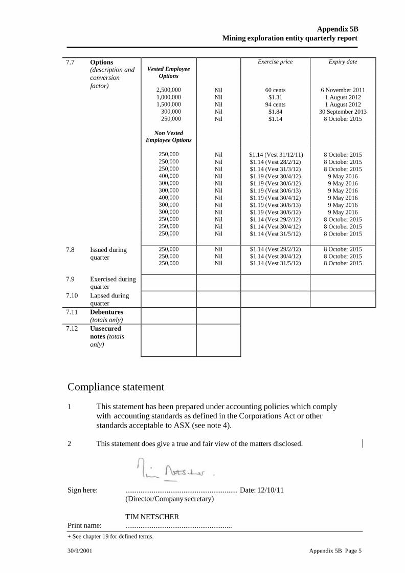
Appendix 5B




7.7 Options

Vested Employee

Options

Nil

Exercise price Expiry date

(description and

conversion

factor) 2,500,000 60 cents 6 November 2011

1,000,000 Nil $1.31 1 August 2012

1,500,000 Nil 94 cents 1 August 2012

300,000 Nil $1.84 30 September 2013

250,000 Nil $1.14 8 October 2015

Non Vested

Employee Options

250,000 Nil $1.14 (Vest 31/12/11) 8 October 2015

250,000 Nil $1.14 (Vest 28/2/12) 8 October 2015

250,000 Nil $1.14 (Vest 31/3/12) 8 October 2015

400,000 Nil $1.19 (Vest 30/4/12) 9 May 2016

300,000 Nil $1.19 (Vest 30/6/12) 9 May 2016

300,000 Nil $1.19 (Vest 30/6/13) 9 May 2016

400,000 Nil $1.19 (Vest 30/4/12) 9 May 2016

300,000 Nil $1.19 (Vest 30/6/13) 9 May 2016

300,000 Nil $1.19 (Vest 30/6/12) 9 May 2016

250,000 Nil $1.14 (Vest 29/2/12) 8 October 2015

250,000 Nil $1.14 (Vest 30/4/12) 8 October 2015

250,000 Nil $1.14 (Vest 31/5/12) 8 October 2015

7.8 Issued during 250,000 Nil $1.14 (Vest 29/2/12) 8 October 2015

quarter 250,000 250,000

Nil Nil

$1.14 (Vest 30/4/12) $1.14 (Vest 31/5/12)

8 October 2015 8 October 2015

7.9 Exercised during quarter

7.10 Lapsed during quarter

7.11 Debentures

(totals only)

7.12 Unsecured

notes (totals

only)

Compliance statement

1 This statement has been prepared under accounting policies which comply

with accounting standards as defined in the Corporations Act or other

standards acceptable to ASX (see note 4).

2 This statement does give a true and fair view of the matters disclosed.

Sign here: ............................................................ Date: 12/10/11

(Director/Company secretary)

TIM NETSCHER

Print name: .........................................................

Appendix 5B




Notes

1 The quarterly report provides a basis for informing the market how the entity’s

activities have been financed for the past quarter and the effect on its cash position.

An entity wanting to disclose additional information is encouraged to do so, in a note

or notes attached to this report.

2 The “Nature of interest” (items 6.1 and 6.2) includes options in respect of interests in

mining tenements acquired, exercised or lapsed during the reporting period. If the

entity is involved in a joint venture agreement and there are conditions precedent

which will change its percentage interest in a mining tenement, it should disclose the

change of percentage interest and conditions precedent in the list required for items

6.1 and 6.2.

3 Issued and quoted securities The issue price and amount paid up is not required in

items 7.1 and 7.3 for fully paid securities.

4 The definitions in, and provisions of, AASB 1022: Accounting for Extractive

Industries and AASB 1026: Statement of Cash Flows apply to this report.

5 Accounting Standards ASX will accept, for example, the use of International

Accounting Standards for foreign entities. If the standards used do not address a topic,

the Australian standard on that topic (if any) must be complied with.

== == == == ==

Documents

Mandatory management forecasts and lender expectations