Managing the Product Development Process: a Simulation Study

Tijdschrift voor Economie e n Management Vol. XLII, 4, 1997

Managing the Product Development Process:

a Simulation Study

by M. R. LAMBRECHT" and M. QUARTIER*

1. INTRODUCTION

Recent changes in the competitive environment make the capability of introducing new products faster and on time very important. Cus- tomers are demanding more customization and responsiveness, new technologies are proliferating at an increasing rate and consequently product life cycles are getting shorter. Evidence suggests that there are significant penalties for not introducing new products on time (Hendricks and Singhal(1997)). While the time needed to work out a concept to a new product, call it processing time, is often relatively short, most companies deal with extremely long times to market, call it the tetal respense time. This is due t e the highly stochastic nature of the development process creating delays and detours in downstream product development activities. Some researchers (see, e.g., Burchill and Fine (1997)) quite rightly state that too much emphasis on the time-orientation creates an environment where pressure for progress encourages development teams to conduct incomplete analysis. A rel- ative emphasis on the market orientation on the other hand may increase the design objective credibility and comnitment but may increase the time required in concept development. This is why we focus in this paper on a well balanced aggregate project plan. Compa- nies always engage in multiple concurrent projects, so we have to man-

' Department of Applied Economics, K.U.Leuven, Leuven. We would like to thank Prof. ICoen Dehackere (K.U.Leuven) for hls helpful suggestiolls and comments. This research was supported by the Tractebel Chair (K.U.Leuven).

age the total workload. We will pay special attention to the release decision of new projects, the size of development teams, the importance of cross-functional teams, the emphasis on the early stages of the development cycle, the introduction of variability reduction tech- niques and the management of bottleneck resources. All of these factors affect the length of the development cycle.

Queueing theory is a methodology which is used to predict in quantitative terms the delays that occur when jobs (projects) compete for processing resources. Many useful insights can be obtained from queueing, but a realistic modeling of the product development process in- volves so many specific characteristics that queueing theory may not be the best way to approach the problem. It is not the purpose of this paper to elaborate on this issue but one example suffices to illustrate the difficulty. In conventional queueing network theory, services are provided in a sequential fashion at specified work centers or stations. In product development projects, however, the simultaneous performance of tasks is very important. This results in the so-called fork and join constructs. A fork occurs whenever several tasks are allowed to begin at the same time. A join node, on the other hand, corresponds to a task that may not be initiated until several other tasks have been completed. These dependencies or synchronization constraints created by the fork and join constructs make this type of queueing networks highly intractable. We refer to Nguyen ((1993), (1994)) for an in-depth treatment of this topic. To finish this paragraph on the meth- odological problems we can conclude that computer simulation seems to be the only satisfactory method that can be used to model the product development process, so that we can analyze in quantitative terms the delays that occur. Consequently, the methodology used in this paper is simulation. We use the Taylor I1 Simulation Software (1993). We refer to the excellent papers of Adler et al. ((1995), (1996)) where the simulation approach is applied to project management. In this paper we both confirm and extend the major findings from Adler et al. ((1995), (1996)), although we use a different model representation.

The paper is organized as follows. We give a formal description of the model in section 11. We refer to it as the base case. In section I11 we describe the simulation results obtained for the base case. In section IV we extend the base case in order to test various aggregate project plan improvement schemes. Finally, some concluding remarks are given in section V.

11. MODEL DESCRIPTION: THE BASE CASE

A. The model

There are several similarities but also important differences between manufacturing operations and knowledge work such as product development. Both can be viewed as stochastic processing networks. In product development a work center is a pool of employees who carry out a specific phase of the product development process. Figure 1 lays out the typical phases of product development. Note that we assume in the base case a simple sequential arrangement. This assumption will later on be relaxed. The typical phases are: concept development (market opportunities, conceptual design, target market, financial impact,...), product specifications (technical possibilities, product requirements, customer needs,...), prototype cycle (the design-build- test cycle, prototyping, tests that simulate product use,...), process development (the design of the production process, tools and equip- ments needed,...), pilot production (individual components, built and tested on production equipment, are assembled and tested as in the factory), and finally the release decision (the conclusion of the detailed engineering phase development is marked by a release or a sign off that signifies that the final design meets requirements). We refer to McGrath et al. (?992), and Wheelwright and Clark ((3 992a), (199213)) for a more detailed description of the development stages. Note that the phases we use can be easily changed. We view each development project (job) as a collection of tasks to be performed by specified resources (designers). These tasks can now be partitioned into phases (cells). This partitioning can be company specific. The cells can oper- ate sequentially or simultaneously (see section IV). By buffering the different phases, most of the undesirable effects of uncertainty can be mitigated.

The modeling of the design team is done as follows. The core resources are the product and process designers and technicians who dedicate their time to development tasks during the various phases of a project. We distinguish three major design groups: marketers, engineers and manufacturers. We assume they make up a pool. In the base case we assume that the pool consists of 27 members (6 marketers, 3 2 engineers and 9 manufacturers). From engineering, one needs good designs, well-executed tests, high-quality prototypes; from mar- keting, thoughtful product positioning, solid customer analysis; from

FIGURE 1

The phases of a project development.

manufacturing, capable processes, skillful pilot production, etc.. In the base case, we assume a functional organization: only marketers are involved in the concept development phase, only engineers in the prototyping phase and e.g. only manufacturers are involved in the process development phase. Because of this functional approach (over- the-wall approach), the design is accomplished somewhat in isolation and this results in a second major complicating factor, namely the existence of rework and many design loops. This, in turn, results in a siower process and a waste of resources. In this case, we distinguish four types of iterations (see Figure 1). First, we have the design-build- test loops in the prototyping phase. Second we have the process development-prototype loop. The manufacturers may indeed consider the model as unfeasible from a manufacturing point of view. Third, the pilot production-process development loop, and fourth the release- product specification loop. It is perfectly possible that at the final

stage, of the development process, marketers may come to the conclusion that the product does not meet customer requirements (e.g. an important customer criticizes the functionality of the proposed product). As a result, the process starts all over again, redefining product specifications. An advantage of our way of modeling the designers (as a pool) is that it allows us to test various allocation strategies. We can allocate designers so that we can measure the impact on total response time of a functional setting or of a cross-functional setting. We can easily measure the impact of the size of groups on the total response time.

To conclude: the model described above allows us to test a family of design and control mechanisms through the concepts of partitioning (the grouping of development tasks in different development phases performed sequentially or concurrently) and the allocation (the size of design teams, functional teams or cross-functional teams). More- over, we can study the effects of variability (demand variability, stochastic processing times, rework loops, ...) on system performance.

B. Types of projects

In our simulation model, we allow different types of development projects. Different categorization criteria can be used for project types, we opt for the topology ifitroduced by Wheelwright and Clark (1992b). They make a distincti~n between derivative, breakthrough axd platform projects.

Consider e.g. derivative projects. These are projects requiring mi- nor design changes, they range from cost-reduced versions of existing products to add-ons or enhancements for an existing production process (e.g. new packaging, minor change in materials used, improved reliability, .. .).

Another category are the breakthrough projects at the other end of the spectrum. These projects involve significant changes resulting sometimes in products that are fundamentally different from previ- ous generations (new technologies, new revolutionary manufacturing processes, ...).

In the middle of the development spectrum, we have the platform projects. Platform projects offer improvements in cost, quality and performance over preceding generations. They introduce improvements across a range of performance dimensions - speed, functionality, size, weight. In this case, we will consider derivative and plat-

form projects, each requiring different processing times for the various stages.

C. Data

At first sight the collection of data seems to he an insurmountable prohlem. It is argued that knowledge work is not repeatable and that there is a total lack of standardization. Adler et al. ((1995), (1996)) conclude, after studying a dozen companies, that accurate estimates of e.g. processing times and project interarrival times can be reason- able well estimated, based on projects' activity histories. Detailed analysis of development projects reveals that many tasks and sequences of tasks are the same across projects and that there are a lot of similarities and even standardization. In order to test our simulation model, we surveyed the literature describing real-life development projects. Based on this survey we constructed a representative data set. We ad- vise the reader to consult Adler et al. (1995) for more details on the estimation issue.

Let's first summarize the data for the platform projects. For a summary see Figure 2. Platform projects have an interarrival time of 27.52 (working) days. More specifically, there is a 60 % chance of an interarrival time of 25 to 40 days, 30 % chance of an interarrival time of 20 to 25 days, 5 % chance of an interarrival time of 12 to 20 days and another 5 % chance of 7 to 12 days. The average processing times (development times) of the various stages are as follow (in working days):

Phase Concept development Product specifications Prototype 0 Design

e Build Test

Process development Pilot production Release decision

time 6.30 days 3.50 days 7.00 days 7.47 days 4.60 days 8.35 days 7.72 days 6.13 days

scv 0.085 0.296 0.088 C.069 0.120 0.083 0.106 0.079

The last column shows us the squared coefficient of variation (SCV). This parameter gives us an idea of the type of distribution and is defined as the ratio of the variance to the squared processing time.

The allocation of our designers (functions) over the stages of a platform project is as follows:

FIGURE 2

Summary of the data for platform projects. 27.52

Piololype Cycle 4.hn 1.85

Function

Marketers Engineers Engineers Engineers Engineers Manufacturers Manufacturers Marketers

Phase

Concept development Product specifications Prototype s Design

e Build Test


Number of people

3 3 5 5 5 4 4 4

Next, we discuss the recycle (loops) probabilities. Loop 1 (prototype):

After a first run of the prototype cycle there is a 70 % chance that we have to repeat the cycle. After a second run, this probability is reduced to 40 % chance. During a loop the processing times are shorter than during the first run:

Design: 2.95 days Build: 2.45 days Test: 1.85 days

Loop 2 (Process development - Prototyping): After a first run through the process development stage, there is a 40 % chance that the model will be returned to the prototype lab. After the second run, this probability is reduced to 30 %. During an iteration, the processing time of the process development phase is reduced to 2.58 days.

Loop 3 (Pilot production - Process development): The loop probability is 60 % after a first run and 20 % in subsequent runs. The pilot production processing time during a loop is 4.00 days.

Loop 4 (Release decision - Product specifications): The probability that the product will fail in the final test is 60 % (in subsequent iterations 15 %). During a loop the processing time of the release decision is 1.85 days and the product specification stage can be done in 3.47 days.

The data for the derivative projects are sumiinarized in Figure 3. The times needed for the different phases during the first loop are given in large bold figures. The time it takes to run through a stage during the subsequent loops is given in small figures. The probability of loops is also given in bold figures during the first iteration and in small figures during the following iterations.

In order to approach steady-state conditions, we have to simulate over a lozg period. During the simulation period 2000 platform projects and 2680 derivative projects are launched. This covers a simulation period of 220 years (assuming 250 working days per year or 55000 days over a 220 year time horizon). In more realistic terms this comes down to an average of 9.09 platform projects per year and 12.18 derivative projects per year.

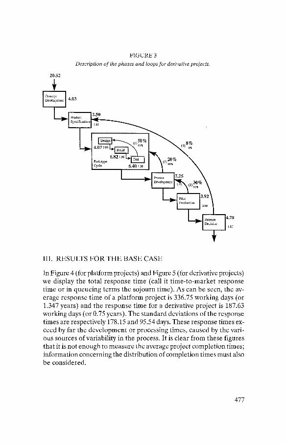
FIGURE 3

Description of the phases and loops for derivative projects.

111. RESULTS FOR THE BASE CASE

In Figure 4 (for platform projects) and Figure 5 (for derivative projects) we display the total response time (call it time-to-market response time or in queueing terms the sojourn time). As can be seen, the average response time of a platform project is 336.75 working days (or 1.347 years) and the response time for a derivative project is 187.63 working days (or 0.75 years). The standard deviations of the response times are respectively 178.15 and 95.54 days. These response times ex- ceed by far the development or processing times, caused by the various sources of variability in the process. It is clear from these figures that it is not enough to measure the average project completion times; information concerning the distribution of completion times must also be considered.

FIGURE 4

Respoizse tinte distiibution of theplatfoirnprolects.

0 100 200 300 400 500 600 700 800 900 1000 1100 120013001400150016001700

response hme

FIGURE 5

Response time dlstributioiz of the derivatzveprojects.

. . . . . . . . . . . . . . . . . . . . . . . . . . . . . . . . . . . . . . . . . . . . . . . . . . . ................................ _. ........ .. ........................................... . . . . . . . . . . . . . . . . . . . . . . . . . . . . . . . . . . . . . . . . . . . . . . . . . . . ................................................................................ . . . . . . . . . . . . . . . . . . . . . . . . . . . . . . . . . . . . . . . . . . . . . . . . . . ......... ........ . I . . ..... . . I . . ...... . I . . ....... , I . . ....... I . . ..... . . I . . ....... I . . ...... . . . . . . . . . . . . . . . . . . . . . . . . . . . . . . . . . . . . . . . . . . . . . . . . . . . ................................. -. .................................................... . . . . . . . . . . . . . . . . . . . . . . . . . . . . . . . . . . . . . . . . . . . . . . . . . . . .........,.........#......... ...... . . . i i . , . ........a....... . . . . . . . . . . . . . . . . . . . . . . . . . . . . . . . . . . ......... : ......... : ......... : ....a.... : ......... : ......... : ........ . . . . . . . . . . . . . . . . . . . . . . . . . . . . . . . . . . . . . . . ................... . . . . . . . . . . . . . . . . . . . . . . . . . . . . . . . . . . . . . . . . . . . . . . . . . . . . . . . . . . . . . . . . . . . . . . . . . . . . . . . . . . . . ........ - ..................................................... . . . . . . . . . . . . . . . . . . . . . . . . . . . . . . . . . . . . . . . . . . . . . . . . . . . . . . . . ...... ...I.. .... . . . I . . ...... . I . . .:... . I . . ...... . . . . . . . . . . . . . . . . . .

0 50 100 150 200 250 300 350 400 450 500 550 600 650 700 750 800 850

response time

An important factor (besides variability) determining the response time is the total workload at the various stages. We therefore measure the utilization level for each stage. This utilization level depends

on several factors: the processing time, the number of iterations and the availability of product developers. Let's analyze this in greater de- tail. Over the simulation period (220 years) we launched 2000 platform projects. How many projects does this represent e.g. for the prototype phase? We know that 70 % (or 1400 projects) return to the design step after being tested the first time. After a second test 40 % of those 1400 projects (or 560) fail again and must go back to the design step, 40 % of which will fail again in the prototype cycle. Moreover, after the process development phase projects can be rejected again and the same holds after a negative release decision. If we treat this routing as Markovian, one can easily compute the total number of projects that must be handled during the prototype phase. In our case this comes down to 6888 platform projects (3.44 times the original arrival frequency) and 5276 derivative projects (1.96 times the original frequency). If we multiply these numbers by the respective processing times we obtain a 83.45 % utilization for the design step (90.93 % for the build step and 69.32 % for the test step). This illustrates how the workload boosts due to the iteration problem. The utilization rates (see the column under the heading utilization p are summarized in the table below.

But there is more involved, delays can also be created due to the unavailability of technicians or designers who make up the pool. To illustrate this with an example, consider the design step in the prototype phase. It takes (for platform projects) on average 7 days to per- form this task. From the detailed simulation results we learn that it takes on average 8 days to finish this step. This extra time is caused by the temporary unavailability of engineers. The project was blocked for one extra day on average. This means that the availability for this work- station is not 100 % but only 87.5 % (7.0018.00). This in turn means that the effective utilization level will be higher than the earlier mentioned 83.45%. The correct effective utilization is now 92 % as can be seen from the table below (see column under the heading effective utilization p *). Effective utilization is the correct measure that we have to employ in order to detect the true bottlenecks (observe the bottleneck shift in the table below).

This discussion brings us to another important issue, namely the size of development teams. Teams that are too large may actually harm the effectiveness of the communication. But there is another important negative side effect. When the size of a development team is too large, then the probability that one can bring the team together to

work on a project will decrease. This in turn will decrease the availability and consequently increase the effective utilization. This in turn will result in more delays and more projects in process. The size of the various development teams is a crucial control parameter. The average utilization of our development teams is:

Marketers: 47,85 % Engineers: 81.62 % Manufacturers: 67.06 %

Effective utilization

P * 46% 42% 92% 97% 77% 94% 74% 57%

Phase

Concept development Product specifications Prototype Design

Build Test


Another interesting statistic is the average number of projects in process (projects-in-process). For our case there are 22 projects on average in process. In the next section we will analyze the impact on time-to-market if we decide to take fewer projects at a time.

From the above discussion we learn that the response time distribution is influenced by variability and by effective utilization. We did not focus our discussion on the variability in processing times itself (which of course is also important), but we rather addressed the issue of variation in workloads due to the existence of design loops. Sec- ond, the concept of effective utilization was introduced to detect the real bottlenecks. In the next section we will extend this base case and suggest various improvement strategies.

Utilization

P 42.11% 35.68% 83.45% 90.93% 69.32% 93.18% 74.34% 51.02%

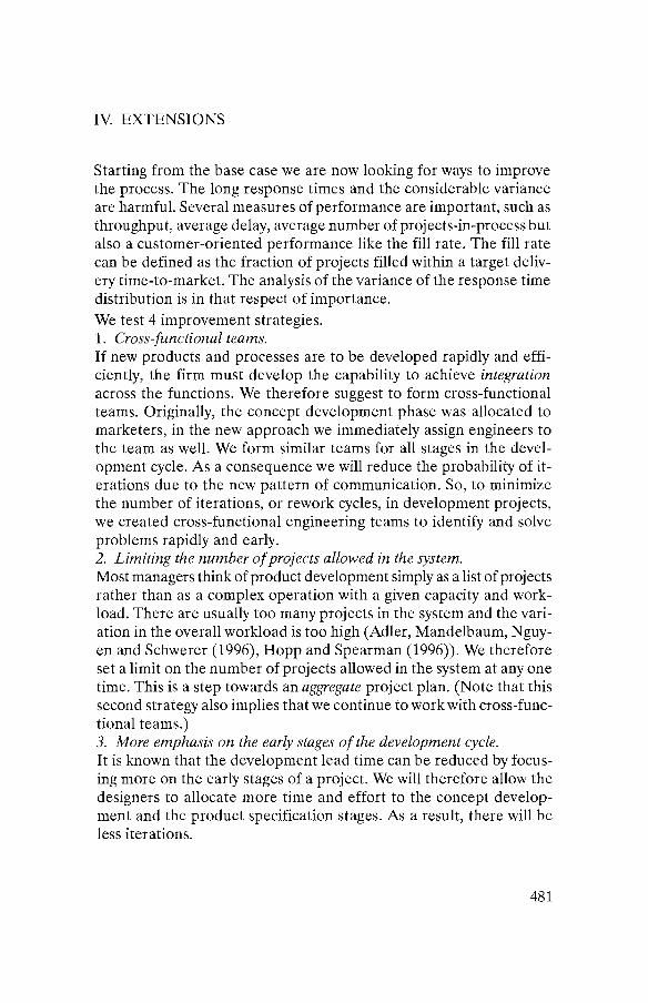
IV. EXTENSIONS

Starting from the base case we are now looking for ways to improve the process. The long response times and the considerable variance are harmful. Several measures of performance are important, such as throughput, average delay, average number of projects-in-process but also a customer-oriented performanice like the fill rate. The fill rate can be defined as the fraction of projects filled within a target deliv- ery time-to-market. The analysis of the variance of the response time distribution is in that respect of importance. We test 4 improvement strategies. 1. Cross-functional teams. If new products and processes are to be deveioped rapidly and effi- ciently, the firm must develop the capability to achieve integration across the functions. We therefore suggest to form cross-functional teams. Originally, the concept development phase was allocated to marketers, in the new approach we immediately assign engineers to the team as well. We form similar teams for all stages in the development cycle. As a consequence we will reduce the probability of iterations due to the new pattern of communication. So, to minimize the number of iterations, or rework cycles, in development projects, we created cross-functional engineering teams to identify and solve problems rapidly and early. 2. Limiting the number ofprojects allowed in the system. Most managers think of product development simply as a list of projects rather than as a complex operation with a given capacity and workload. There are usually too many projects in the system and the variation in the overall workload is too high (Adler, Mandelbaum, Nguy- en and Schwerer (1996), Hopp and Spearman (1996)). We therefore set a limit on the number of projects allowed in the system at any one time. This is a step towards an aggregate project plan. (Note that this second strategy also implies that we continue to work with cross-functional teams.) 3. More emphasis o n the early stages of the development cycle. It is known that the development lead time can be reduced by focus- ing more on the early stages of a project. We will therefore allow the designers to allocate more time and effort to the concept development and the product specification stages. As a result, there will be less iterations.

4. Betterpatterns of communication. Up till now we assumed that the design teams were operating in a serial mode of interaction. The downstream group waits to begin its work until the upstream group has completely finished its design. This batch style (see Wheelwright and Clark, 1992a) of communication may be replaced by a more integrated problem solving style so that development teams can work simultaneously.

For all improvement strategies mentioned above, we will keep the throughput (number of projects finished within a specified time horizon) constant. This makes it easier to interpret the simulation results.

A. Cross-functional teams

As mentioned earlier, a first step towards an aggregate project plan is to reallocate the members of the project team. This means that members of each group (marketers, engineers and manufacturers) are involved in almost every step of the development process. As a consequence the team size is larger, but on the other hand there is a reduction of the number of loops. A manufacturer e.g. can specify during the product specifications phase what can and what can't be achieved on the production floor. We first describe the modified model, next, we discuss the simulation results.

In the table below the new team allocations are summarized (Note that the size of the total design team is still limited to 27 members)

These data are related to the platform projects. The teams for the development of derivative projects are extended in a similar way.

Phase

Concept development Product specifications Prototype . Design

Build Test


Number of

people 5 6 7 8 6 5 6 4

Function

Marketers, Engineers,Manufacturers Engineers, Marketers, Manufacturers Engineers, Manufacturers, Marketers Engineers, Manufacturers, Engineers , Manufacturers Manufacturers, Engineers Manufacturers, Engineers, Marketers Marketers, Manufacturers, Engineers

Due to the new pattern of communication, one may expect a decrease in the number of design iterations. We summarize the recycle probabilities (for the platform projects) below: Loop 1 (prototype):

The chance that a prototype has to be redesigned after the first test has decreased from 70 % to 30 %. The probability that the prototype needs another revision after the second cycle is reduced to 20 %.

Loop 2 (Process development - Prototyping): After a first run, 20 % of the projects will be found not pro- cessible and will be returned to the prototype cycle. During the next trials, the process development will fail for 15 % of the projects.

Loop 3 (Pilot production - Process development): After a first run through the pilot production stage, there is a chance of 30 % that problems will arise and that the project has to be returned to the process development stage. After the second run, this probability is reduced to 10 %.

Loop 4 (Release decision - Product specifications). The chance that the release decision is negative is 20 %. In the subsequent iterations, this probability will be reduced to 8 %.

In the table below we summarize the data for derivative projects.

These new parameter settings resulted in the following simulation outcomes. First examine the total response time distributions in Fig- ures 6 and 7.

We clearly observe different distributions as compared to the base case. The average response time for platform projects is 213.68 days (compared to 336.75 days) and for derivative projects we obtain an

Loop 1 2 3 4

Probability of loops After first run

15% 8% 10% 4%

After subsequent runs 6% 5% 5% 3%

average of 145.51 days (compared to 187.63 days). The standard deviation for platform projects is 120.44 days and for derivative projects 72.68 days. The average number of projects in process also decreased from 22 projects to 15 projects.

The number of iterations drastically decreased. In the prototype phase e.g. 3642 platform projects were processed (over the total simulation period) as compared to the 6888 in the base case. This auto- matically results in lower utilization rates (see table below). But the effective utilization rates are fairly high (see table below)

This can be explained as follows. The utilization of the development teams drastically increased: Marketers: 62.11 %; Engineers: 86.52 % and Manufacturers: 83.57 %, basically because the designers are now involved in almost every phase. That also means that the availability of the designers decreased and this in turn results in fairly high effective utilization rates. Overall, however, the introduction of cross- functional teams elevated a number of bottlenecks, explaining partly the shorter response times. The reduction of the number of loops clearly reduces the variability of the workload and this has a positive impact on the response times.

FIGURE 6

Response time distribution of theplatfonnpi-ojects working with cross-functional teams.

. . . . . . . . . . . . . . . . . ............................................................................... . . . . . . . . . . . . . . . . . . . . . . . . . . . . . . . . . . . . . . . . . . . . . . . . . . . ............................. I . . ..... . . I . . ...... ., ......... I . . ....... , ... . . . . . . I . . ...... . . . . . . . . . . . . . . . . . . . . . . . . . . . . . . . . . . . . . . . . . . . . . . . . . . . ........................................................................................ . . . . . . . . . . . . . . . . .

0 50 100 150 200 250 300 350 400 450 500 550 600 650 700 750 800 850

response time

FIGURE 7

Resporise tinie distribution of the derii/ntiveprojects working with cross-fitnctional teanzs.

....... ......... ....... ....... ......... ....... ...... . . . S . . , , . . I . . , I . . I . . . . . . . . . . . . . . . . . . . . . . . . . . . . . . . . . . . . . . . . . . . . ........................................................................ . . . . . . . . . . . . . . . . . . . . . . . . . . . . . . . . . . . . . . . . . . .............. , ......... , ............................. , ......... , ........ . . . . . . . . . . . . . . . . . . . . . . . . . . . . . . . . . . . . . . . . . . . . . . . . . . . . . . . . . . . . . . . . . . . . .................................................................... . . . . . . . . . . . . . . . . . . . . . . . . . . . . . . . . . . . . . . .

. . . . . . . . . . . .

0 50 100 150 200 250 300 350 400 450 500 550 600 650 700 750 800 850

response time

Phase Concept development Product specifications Prototype 0 Design

0 Build Test

Process development Pilot development Release decision

Utilization p 43.12% 27.87% 57.50% 70~35% 55.28% 76.07% 56.87% 46.85%

Effective utilization p * 52% 45 % 76% 95% 75 % 92% 81% 54%

B. Limiting the number of projects in process

In the base case simulation, the product development organization had on average 22 projects-in-process. It is clear that it is useless to start new projects if the organization is already overloaded. Launching another project will only create more stress, more unfinished projects on time and longer development cycles without improving the throughput. That's why many researchers favor some sort of input control. We simulate the following strategy: we decide not to launch a new project when the level of unfinished projects rises above a pre-set cutoff lev-

el. The cutoff level is set equal to 13 projects. If a new project arrives, we count the number of projects in the different phases, if that number is less than 13, the project can be released. By imposing an upper limit on the number of projects we impose a so-called constant work- in-process strategy (CONWIP, see Hopp and Spearman (1996), Spear- man and Zazanis (1992) and Spearman et al. (1990)). Note that the upper bound is set equal to 13, because this cutoff level does not hurt the throughput (a number of trial and error simulation runs is required to find this cutoff level). Also note that we continue working with the data specified in section 1V.A.

The simulation results indeed confirm the theoretical finding: both the expected response time and the standard deviation are reduced. The expected response times for platform projects and derivative projects are now respectively 173 days and 124 days. Moreover, the standard deviations are drastically reduced to 71.28 days and 42.02 days respectively.

We have, however, to interpret this favorable impact with care. By implementing such apull policy, we must realize that we will always have projects on the shelfwaiting to be released. The overall response time, i.e. including the waiting time of projects on the shelf may actually increase. Since we restrict the entrance of projects into the development organization, we create a more constrained system than the traditional open system (i.e. a system not imposing a cutoff level). That is confirmed by our simulation experiment. The overall response time indeed increases (274.39 days for platform projects and 223.52 days for derivative projects). Separating the external demand process from the development process itself offers management the opportunity to be more careful with respect to the selection of projects. We quote from Adler et al. (1995): "Input control policies look particularly at- tractive if management can select projects according to their probabilities of success". This highlights again the importance of an aggregate project plan.

C. More emphasis on the early stages of the development cycle

A survey of the product development literature and an analysis of existing practice reveal that the front-end phases of the product development process are extremely important. The lack of design objective credibility (Burchill and Fine (1997)) during the early stages of the process results in delays and detours in downstream product de-

velopment activities. It is therefore suggested to spend more time during the early stages of the process. More specifically, we increase the average duration of the concept development stage (for platform projects) from 6.30 days to 8.85 days and the processing time of the product specification step is set equal to 6.07 days (instead of 3.50 days). For derivative projects we set the processing times equal to 6.05 days (concept development) and 4.07 days (product specification) respectively. Except for the loop probabilities we use the same data as described in section 1V.A and 1V.B.

It is expected that the increased effort during the early stages will result in fewer iterations. This is expressed in the tables below.

Loop 1 2 3 4

The simulation results now reveal drastic reductions in the response times. The distribution of the platform projects is now characterized by an average of l11 days and a standard deviation of 35.22 days. The distribution of the derivative projects reflects a mean response time of 110.1 days and a standard deviation of 38.31 days.

Loop 1 2 3 4

Probability of loops (platform projects) After first run

10% 5% 10% 5%

Probability of loops (derivative projects)


After first run 5% 2% 3% 2%


A closer look at the utilization rates reveal a more evenly spread workload:

Investments to relieve bottlenecks (less iterations through an increased effort at the early stages of the process) yield disproportion- ately large time-to-market benefits.

D. Betterpatterns of cornrnunication

Effective utilization P * 87% 65 % 63% 75 % 64 % 85 % 78 % 63%

Phase Concept development Product specifications Prototype a Design

Build a Test

Process development Pilot development Release decision

The generic product development process in Figures 2 and 3 suggests a simple serial structure, i.e. the downstream group waits tc begin its work until the upstream group has completely finished its design. It is however advisable to work simultaneously (concurrent engineering). Wheelwright and Clark (1992b) propose an integrated problem solving, linking the upstream and downstream groups in time and in the pattern of communication. We quote (Wheelwright and Clark (1992b)): "In this mode, downstream engineers not only participate in a pre- liminary and ongoing dialogue with their upstream counterparts, but use that information and insight to get a flying start on their own work". We modeled this pattern of communication as follows. We assume that the concept development step and the product specification step can be performed simultaneously. The data are summarized on Figures 8 and 9. We build on the data from section IVC.

Utilization p 61.76% 42.82% 48.36% 62.60% 49.70% 67.97% 49.72% 46.25%

This new mode of operation again results in faster response times. The average response times for platform projects now equals 100.33 days (standard deviation 36.45 days) and for derivative projects we obtain an average of 87.33 days (standard deviation 30.63 days).

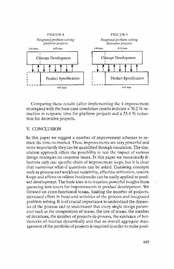
FIGUUR S FIGUUR 9

It~tegratecl problem solving O~tegratecl problem solving plotforin projects derivative projects

2.83 days 6.02 days 1.90days 4.15 days

cdncept Development

I I I Product Specification Product Specification I

6.07 days 4.07 days

Comparing these results (after implementing the 4 improvement strategies) with the base case simulation results indicate a 70.2 % reduction in response time for platform projects and a 53.4 % reduction for derivative projects.

V. CONCLUSION

In this paper we suggest a number of improvement schemes to reduce the time-to-market. These improvemerzts are very powerful and more importantly they can be quantified through simtilation. The simulation approach offers the possibility to test the impact of various design strategies on response times. In this paper we numerically illustrate only one specific chain of improvement steps, but it is clear that numerous what-if questions can be asked. Queueing concepts such as process and workload variability, effective utilization, rework loops and efforts to relieve bottlenecks can be easily applied to product development. The basic idea is to translate powerful insights from queueing into levers for improvements in product development. We focused on cross-functional teams, limiting the number of projects, increased effort in front-end activities of the process and integrated problem solving. It is of crucial importance to understand the dynamics of the process and to understand that every single design parameter such as the composition of teams, the size of teams, the number of iterations, the number of projects-in-process, the existence of bottlenecks all interact dynamically and that an overall aggregate management of the portfolio of projects is required in order to make prod-

uct development effective and efficient. The systems dynamics methodology based on simulation offers a powerful tool for systematically analyzing real life cases.

REFERENCES.

Adler, P.S., Mandelbaum, A., Nguyen, V. and Schwerer, E., 1995, From Project to Process Management: An Empirically-Based Framework for Analyzing Product Development Time, Marlageiner~t Science 41, 458-484.

Adler, PS., Mandelbaum, A., Nguyen, V. and Schwerer, 1996, E., Getting the Most out of Your Product Development Process, Haward Bzlsiness Review, March-April, 134-152.

Burchill, G. and Fine, C.H., 1997, Time Versus Market Orientation in Product Concept De- velopment: Empirically-Based Theory Generation, Mar~ageinenr Science, 43, 465-478.

F&H Simulations, 1993, Taylor I1 Simulation Software: Simulation in Manufacturing and Logistics, (F&H Logistics and Automation B.V., Utrecht).

Hendricks, K.B. and Singhal, VR., 1997, Delays in New Product Introductions and the Mar- ket Value of the Firm: The Consequences of Bcing Late to the Market, Management Scietz- ce, 43, 422-436.

Hopp, W. and Spearman, M,, 1996, Factory Physics: Foundations of Manufacturing Mana- gement (Irwin, Homewood Ill.).

McGrath, M, , Anthony, M. and Shapiro, A., 1992, Product Development: Success Through Product and Cycle-Time Excellence (Butterworth-Heinemann, Boston).

Nguyen, V., 1993, Processing Networks with Parallel and Sequential Tasks: Heavy Traffic Analysis and Brownian Limits, The Annals ofAppliedProbabilily, 3, 28-55.

Nguyen, V., 1994, The Trouble with Diversity: Fork-Join Networks with Heterogeneous Customer Population, Tile Annals ofApplied Probability, 4, 1-25.

Spearman, M. And Zazanis, M,, 1992, Push and Pull Production Systems: Issues and Com- parisons, Operations Research, 40, 521-532.

Spearman, M,, Woodruff, D. And Hopp, W., 1990, CONWIP: a Pull Alternative to Kan- ban, I~~ ter i~ar iona l , Iour~~al nf Plwductio?~ Researclz. 28. 879-894.

Wheelwright, S. and Clark, K., 1992a, Revolutionizing Product Development (The Free Press, New York).

Wheelwright, S. and Clark, K., 1992b, Creating Project Plans to Focus Product Develop- ment, Haward Business Review, March-April, 70-82.

Documents

Managing the Product Development Process: a Simulation Study