i

Managing Performance and Efficiency of a Processor

by

Aditi Jaysing Shinde

A project submitted to the Graduate Faculty of

Auburn University

in partial fulfillment of the

requirements for the Degree of

Master of Electrical Engineering

Auburn, Alabama

December 8, 2012

Keywords: power consumption, energy per cycle, energy efficiency

Copyright 2012 by Aditi Jaysing Shinde

Approved by

Vishwani Agrawal, Chair, James J. Danaher Professor of Electrical and Computer Engineering

Victor Nelson, Professor of Electrical and Computer Engineering

Adit Singh, James B. Davis Professor of Electrical and Computer Engineering

ii

Abstract

Voltage scaling has been a very popular low power design methodology in the industry. Having a quadratic relationship with the power consumed, lowering the supply voltage reduces the supply voltage considerably. But this mars the overall performance of the circuit. Optimizing performance and power simultaneously requires a thorough study of the available resources and tradeoffs possible.

This project looks into one of the most important areas of contemporary research in electrical and computer engineering: energy efficiency [11, 19, 42]. Power and Performance are two conflicting goals a designer has to achieve [25]. With a number of performance oriented devices emerging with a huge demand of power from a fixed capacity battery, using the battery wisely becomes important. This project investigates the existing and suggests a new metric which can be considered while deciding upon the working conditions of the processor for optimal energy efficiency.

Performance of a processor generally refers to its time efficiency. For given architecture, hardware and software, clock frequency (f), i.e., cycles per second (Hz), or cycle rate is the rate of computational work measured in clock cycles done per unit time. In a similar way, we introduce a new measure, cycle efficiency (η) as cycles per joule, or the rate of computational work per unit energy. Characterization of the technology used in a processor allows us to estimate its frequency and cycle efficiency as functions of the supply voltage. This data is useful in managing the operational characteristics of processors, especially those used in mobile or remote systems where both execution time and energy are important.

As an example, we studied the Intel Pentium M processor in 90nm CMOS technology. We assumed 90nm PTM (predictive technology model) because it is available for the required analysis using HSPICE simulation. At the nominal operating voltage of 1.2V we found f = 1.3GHz and η = 15 megacycles/joule. Consider a program that executes in 1.3 billion clock cycles on this processor. If we run the processor at 1.2V, the program will run in 1 second and consume 86.7 joules. For operation at 0.6V supply, we determined f = 350MHz and η = 70 megacycles/joule, resulting in a run time of 4 seconds and consumption of 18.6 joules. We also found that at the extreme, if the processor runs at a subthreshold supply of 200mV, then f = 100MHz and η = 660 megacycles/joule. Now the program will take 13 seconds but will consume only 1.97 joules. Thus, characterization of a processor for frequency and cycle efficiency would allow its operation to be managed according to the time and energy requirements.

iii

Acknowledgments

I would never have completed this project without the support, encouragement and guidance of

many people. I cannot possibly list everyone that helped make my Master’s journey a fulfilling

experience; I will mention just a few.

First and foremost I would like to thank Dr. Vishwani Agrawal, my principal advisor, for his support,

guidance, and encouragement. Working with him was a privilege and a great learning experience. I

would also like to thank Dr. Adit Singh and Dr. Victor Nelson for their support and guidance as members

of my committee. It was an honor to be a part of Auburn University and a privilege to learn from its

professors. I am indebted to my student colleagues at Auburn University for providing a stimulating

environment to learn and grow. I am extremely grateful to Manish Kulkarni for his immense patience

and guidance he offered at every stage of this project.

Finally, I would like to thank my parents Jaysing S., Shobhana S., sister Devika and my friends Ipsitaa,

Sheetal, Rucha, Kalyani, Indraneil and Praveen for their encouragement and support during this work.

iv

Table of Contents

Abstract ....................................................................................................................................................... ii

Acknowledgments ...................................................................................................................................... iii

List of Figures ............................................................................................................................................. .v

1 Introduction .......................................................................................................................................... 1

1.1 Power Dissipation in CMOS circuits………………………………………………………..…………………………....…..2

1.2 Static Dissipation …………………………………………………………………………………………..……………….………...2

1.3 Dynamic Dissipation ……………………………………………………………………………………..…….………….…….....2

2 Performance and Energy Efficiency Metrics ............................................................................... ...…..3

2.1 System Performance Metric ………………………………………………………………………………………………………3

2.2 Execution Time and Performance ………………………………………………………………………………………………5

2.3 Energy Efficiency Metrics ……………………………………………………..……………………………………………………6

3 Characterization of Intel Pentium M for given technology………………………………………………..………………8

4 Limitations ……………………………………………………………………………………………………………………..………………12

5 Conclusion and Future Work …………………………………………………………………………………………….……………13

References ………………………………………………………………………………………………………………………………………....14

v

List of Figures

3.1 Energy HSPICE [1] characterization of 8 bit ripple carry adder in 90m PTM [48]……………..………………8

3.2 Energy per cycle for an Intel Pentium M Processor …………………………………………….………………………….9

3.3 Cycle Efficiency and Frequency plots against supply voltage Vdd……………………………………………………..10

1

Chapter 1

Introduction

One of the principal design constraints that chip designers face today is power. Though Moore’s law permits further increase in number of transistors per chip, power figures restrain them from actually being implemented. Recent efforts in energy aware computing have examined many different ways to reduce power consumption for example [4, 9, 15, 17, 20]. Dynamic power management is one of the most successful design methodology followed for commercial integrated circuits (IC’s) [30]. Normally, supply voltage may be lowered by about 20-30% to reduce the power consumption. However, recently near-threshold and below-threshold voltage operations have been studied. It is found that if the power supply voltage (Vdd) is scaled below the device threshold voltage, small subthreshold currents slowly charge and discharge the circuit’s nodes reducing the dynamic power and leakage power. Hence giving longer battery life [16, 17, 18, 19, 38]. Though the circuit must be operated at rather low clock frequencies in megahertz range.

The reduced power consumption comes with a price, which is either reduced performance or increased area or both. Varieties of processors available today vary from simple machines with modest performance and extremely low power consumption to processors with complex architecture and with huge power dissipation [5, 10]. With the recent increased demand in portability and performance, incorporating the flexibility to operate at various conditions satisfying these demands, becomes inevitable. It becomes important to define new and check into existing metrics for achieving the same.

We can trade off performance in the situations where battery life is limited and the task needs to be completed in fixed amount of energy resource. On the other hand, we can afford a very high performance if the battery is not allowed to be drained through continuous charging. These highlight the two extremes of the best performance and best energy efficient processor operation. Hence it is important to take in consideration the working conditions, available battery charge and performance requirement and optimize it universally.

Power consumption affects various aspects of a computer system and its effects should be considered at all levels. Described below are few aspects which are directly related to power consumption [26, 27].

Battery life: An important consideration for mobile devices is the time span for which the device can be used without recharging or replacing the power source. This can be extended by power efficient designs. The performance, of course, remains another criterion, which may be sometimes traded off for power.

Large scale power consumption: This aspect is not substantial when we talk of an individual desktop computer. When we take into consideration massive arrays of these used in big organizations, the power consumption can be substantial. Small savings in such large arrays can give us fairly large power saving.

2

Thermal issues: Power dissipation leads to heat generation. Excessive heat generation can impact a machine’s reliability and the cooling system cost and power. Besides, there is direct impact on the packaging size and cost.

1.1 Power Dissipation in CMOS Circuits

Power dissipation in CMOS circuits occurs in various ways. The major ways are described in the following section. Point to note is that the power dissipation can never be zero as a small current always flows. Power dissipation can be further divided into static and dynamic power dissipation.

Ptotal = Pdynamic + Pstatic

1.2 Static Dissipation

Commonly known as leakage, is the ‘per cycle energy’ drain in the circuit when there is no activity in the circuit. Main cause for leakage power is the leakage current which flows due to subthreshold conduction. When we scale supply voltage below the threshold value, leakage current increases leading to increased leakage power consumption.

1.3 Dynamic Dissipation

It broadly constitutes of transition and short circuit power. It is formulated as

Pdynamic = Cl Vdd2 f

1.3.1 Transition

Transition power is dissipated when a transistor charges or discharges to change its state from high to low or vice versa. It includes the power consumed due to all the logical activity in the circuit plus the power consumed due to glitches.

1.3.2 Short Circuit

The charging or discharging of CMOS transistor to change state does not happen instantly. There is always some propagation delay while the transistors acquire the required voltages. There is a small period of time during this activity where in both the transistors are conducting. This leads to a small current to flow from the drain to the source and hence dissipate power. This power is majorly dependent on the rise and fall time of the input.

3

Chapter 2

Performance and Energy Efficiency Metrics

Performance has always been an important attribute and deciding factor when it comes to purchasing a new computer. Measuring and hence comparing different computers is vital for the purchaser and hence the designer [27]. There are various goals as to why we consider performance analysis. It helps us in comparing various alternatives and chooses the one which suits our requirement the best. It helps us in finding the set of parameter values which will result in optimum overall performance of the system. Performance analysis assists in determining the impact of a particular feature. Knowing the performance of a system we can set our expectations about its working. On a broader view we can identify relative performances of multiple systems. We can debug performance and alter set of specifications to get best performance [44].

Selecting a performance metric depends on the specific situation, its goals and the cost involved in collecting the required data. A good performance metric should be linear, reliable and should be repeatable. It should be easy to measure, consistent that is its definition should remain same across different systems and different configurations. Performance measure should also be independent of outside influences to avoid corruption of its meaning.

2.1 System Performance Metrics

A wide variety of performance metrics are proposed and used today in the field of computer science. Not all of them are good enough to be used in the industry depending on the qualities defined above. We will have a look at the most common metrics in the following subsection and have a brief evaluation on its stand as a good metric [22].

2.1.1 The Clock Rate

It states the processor’s central clock frequency. The purchaser assumes that a 1.2 GHz system must be faster than a 1 GHz system. This performance metric does not take into consideration the amount of computation actually accomplished in a given clock cycle. It also ignores the processor’s interaction with other subsystems as the memory and input/output. This is a good performance metric when we consider repeatability, consistency and ease of measurement and is independent. However, this metric is highly non linear and unreliable. A faster clock in no way signifies that it runs the programs correspondingly faster. It is in a way misleading.

4

2.1.2 MIPS

We can have metrics which measure the amount of computation performed per unit time. Rate metrics are generally normalized to a common base to make its comparison becomes easier. MIPS is a performance metric developed specifically for computer systems. It directly compares the speed of a system. MIPS stands for Million Instructions (executed) Per Second and is defined as

𝑀𝐼𝑃𝑆 =n

t ∗ 106

Where n is the total number of instructions and t is the time required to execute them. This metric is easy to measure, repeatable and independent but still doesn’t qualify as a very good performance metric as it is not linear and reliable. The main issue with MIPS as a performance metric is that it doesn’t take into account that different processors can perform different amount of computation in a single instruction. The different amount of computation in a single instruction is the core of RISC and CISC processors and renders MIPS as a useless performance metric. 2.1.3 MFLOPS

MFLOP comes as an improvised version of MIPS. MFLOPS stands for Millions of Floating Point Operations executed Per Second and is given as

𝑀𝐹𝐿𝑂𝑃𝑆 =f

t ∗ 106

Where, f is the number of floating point operations executed in t seconds. MFLOPS is more acceptable as floating point operations are more clearly comparable across computer systems than execution of a single instruction. This metric fails when we use it to evaluate a program which does not have a single floating point operation. The program might be doing a very important sorting, swapping or a searching a database type of operation. Also the way in which floating point operations are counted for a program is still questionable. 2.1.4 SPEC

SPEC stands for System Performance Evaluation Cooperative (SPEC) and was founded to standardize actual result of a computer system in typical usage. This group defined a set of integer and floating point benchmark programs that reflected the way majority of work station class computers were used. Most importantly they standardized the methodology for measuring and reporting the performance obtained while executing these programs.

5

2.1.5 QUIPS

QUIP is an acronym for Quality Improvement per Second. This benchmark was developed to analyze th e ’quality of the solution’ which is more meaningful to the user. The quality is defined on the basis of mathematical characteristics of the target problem [22]. Though it is not a general purpose metric, QUIPS is proving to be useful in determining a system’s numerical processing capabilities.

2.1.6 Execution Time

Finally, we are always interested in how quickly the program is executed. Thus the fundamental metric to analyze a system’s performance is the time taken required to execute a given application program. Performance can be measured in various units. The most common unit used is time. Time can be measured in seconds(s), microseconds (μs), nanoseconds (ns), or picoseconds (ps). Second most common unit is clock cycle. It is defined as the period of hardware clock. For a clock frequency of 1 GHZ, we say the clock cycle is of 1 nanosecond.

𝐶𝑃𝑈 𝑡𝑖𝑚𝑒 =CPU clock cycles

clock rate

CPU time is the time taken by CPU to execute a given program. It has two major components, User CPU time and System CPU time. User CPU time is the time taken by CPU to execute instructions of the program where as System CPU time is the time taken by operating system to run the program.

Cycles per instruction (CPI) is another important performance unit. It tells us the average number of clock cycles utilized to execute a computer instruction. We also define Elapsed time (wall clock time) which is the time interval between the start and end of a program.

2.1.7 Synthetic Benchmarks

Synthetic programs are pre dominantly artificial programs that emulate a large set of typical ‘real’ programs. Algol and Fortran (Whetstone benchmark) and Ada and C (Dhrystone benchmark). The major drawback of synthetic benchmarks is that there is no well defined understanding of what a typical instruction mix should be. These benchmarks do not adequately generate meaningful result. In synthetic benchmarks the purpose of rating is defeated when compilers are written to optimize the performance rating.

6

2.2 Execution Time and Performance

Performance is evaluated for a given program or a set of programs. Simplest way to summarize performance of a system is to compute execution time of the various programs used.

𝑃𝑒𝑟𝑓𝑜𝑟𝑚𝑎𝑛𝑐𝑒 =1

Execution time

Arithmetic mean is given as the average of the execution times. This value is always proportional to the total execution time. Arithmetic mean for n such programs is given by

𝐴𝑣𝑔 𝐸𝑥𝑒𝑐𝑢𝑡𝑖𝑜𝑛 𝑡𝑖𝑚𝑒 =1𝑛

�Execution time (program i )𝑛

𝑖=1

Though easy to compute, arithmetic mean is not usually used for measurement. We use Geometric mean which is defined as follow.

𝐴𝑣𝑔 𝐸𝑥𝑒𝑐𝑢𝑡𝑖𝑜𝑛 𝑡𝑖𝑚𝑒 = [�Execution time (program i) ]1/n𝑛

𝑖=1

2.3 Energy Efficiency Metrics

Energy efficiency is the ratio of performance to the amount of energy consumed to achieve that performance. The following section gives an overview of the most common metrics used to quantify energy efficiency of various circuit designs.

Efficiency averaged on n benchmark programs is given by

𝐸𝑓𝑓𝑖𝑐𝑖𝑒𝑛𝑐𝑦 = �(𝑛

𝑖=1

Efficiency i)1/n

Where Efficiencyi is the efficiency for program i. Relative efficiency of a computer system is defined with respect to a reference computer.

7

𝑅𝑒𝑙𝑎𝑡𝑖𝑣𝑒 𝑒𝑓𝑓𝑖𝑐𝑖𝑒𝑛𝑐𝑦 = Efficiency of a computer

Efficiency of reference computer

2.3.1 Et2 Energy and time (square) product.

This is one voltage independent metric and was developed for comparing cross processor analysis. It is proportional to [MIPS3/Power]. Being independent of voltage this metric is highly biased to delay/execution time.

2.3.2 Power × Time (Energy per Operation)

As the name suggests, this metric is calculated/measured for a given operation. It is the product of average power and time duration of the operation. In simpler words, it gives us the electrical energy used for performing a particular operation [18].

Our work focuses on characterizing a processor for a given technology and work out its energy efficiency.

8

Chapter 3

Characterization of Intel Pentium M for given technology

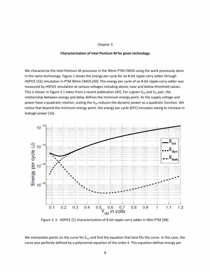
We characterize the Intel Pentium M processor in the 90nm PTM CMOS using the work previously done in the same technology. Figure 1 shows the energy per cycle for an 8-bit ripple carry adder through HSPICE [16] simulation in PTM 90nm CMOS [50]. The energy per cycle of an 8-bit ripple-carry adder was measured by HSPICE simulation at various voltages including above, near and below threshold values. This is shown in Figure 3.1 taken from a recent publication [45]. For a given Vdd and Vth pair, the relationship between energy and delay defines the minimum energy point. As the supply voltage and power have a quadratic relation, scaling the Vdd reduces the dynamic power as a quadratic function. We notice that beyond the minimum energy point, the energy per cycle (EPC) increases owing to increase in leakage power [16].

Figure 3. 1: HSPICE [1] characterization of 8-bit ripple-carry adder in 90m PTM [48].

We interpolate points on the curve for Etot and find the equation that best fits the curve. In this case, the curve was perfectly defined by a polynomial equation of the order 4. This equation defines energy per

9

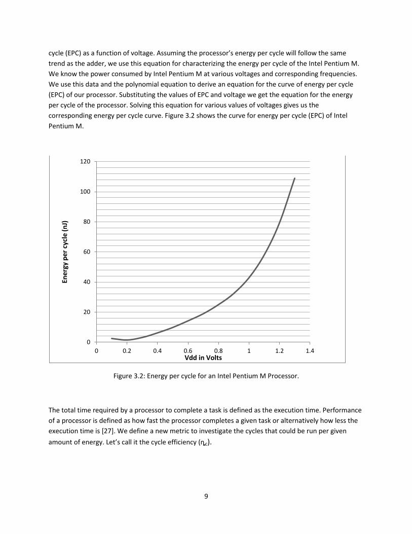
cycle (EPC) as a function of voltage. Assuming the processor’s energy per cycle will follow the same trend as the adder, we use this equation for characterizing the energy per cycle of the Intel Pentium M. We know the power consumed by Intel Pentium M at various voltages and corresponding frequencies. We use this data and the polynomial equation to derive an equation for the curve of energy per cycle (EPC) of our processor. Substituting the values of EPC and voltage we get the equation for the energy per cycle of the processor. Solving this equation for various values of voltages gives us the corresponding energy per cycle curve. Figure 3.2 shows the curve for energy per cycle (EPC) of Intel Pentium M.

Figure 3.2: Energy per cycle for an Intel Pentium M Processor.

The total time required by a processor to complete a task is defined as the execution time. Performance of a processor is defined as how fast the processor completes a given task or alternatively how less the execution time is [27]. We define a new metric to investigate the cycles that could be run per given amount of energy. Let’s call it the cycle efficiency (ȵc).

0

20

40

60

80

100

120

0 0.2 0.4 0.6 0.8 1 1.2 1.4

Ener

gy p

er c

ycle

(nJ)

Vdd in Volts

10

η = 1

energy per cycle

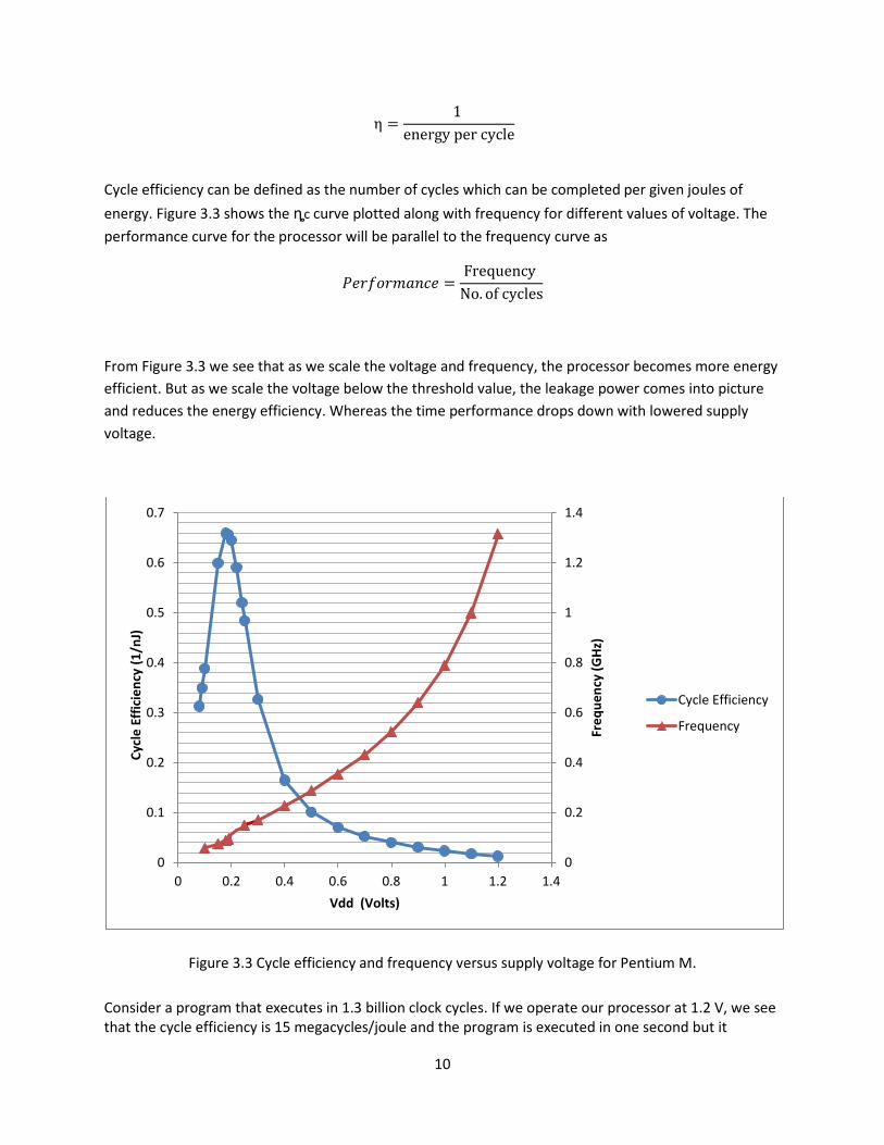
Cycle efficiency can be defined as the number of cycles which can be completed per given joules of energy. Figure 3.3 shows the ȵc curve plotted along with frequency for different values of voltage. The performance curve for the processor will be parallel to the frequency curve as

𝑃𝑒𝑟𝑓𝑜𝑟𝑚𝑎𝑛𝑐𝑒 = Frequency No. of cycles

From Figure 3.3 we see that as we scale the voltage and frequency, the processor becomes more energy efficient. But as we scale the voltage below the threshold value, the leakage power comes into picture and reduces the energy efficiency. Whereas the time performance drops down with lowered supply voltage.

Figure 3.3 Cycle efficiency and frequency versus supply voltage for Pentium M.

Consider a program that executes in 1.3 billion clock cycles. If we operate our processor at 1.2 V, we see that the cycle efficiency is 15 megacycles/joule and the program is executed in one second but it

0

0.2

0.4

0.6

0.8

1

1.2

1.4

0

0.1

0.2

0.3

0.4

0.5

0.6

0.7

0 0.2 0.4 0.6 0.8 1 1.2 1.4

Freq

uenc

y (G

Hz)

Cycl

e Ef

ficie

ncy

(1/n

J)

Vdd (Volts)

Cycle Efficiency

Frequency

11

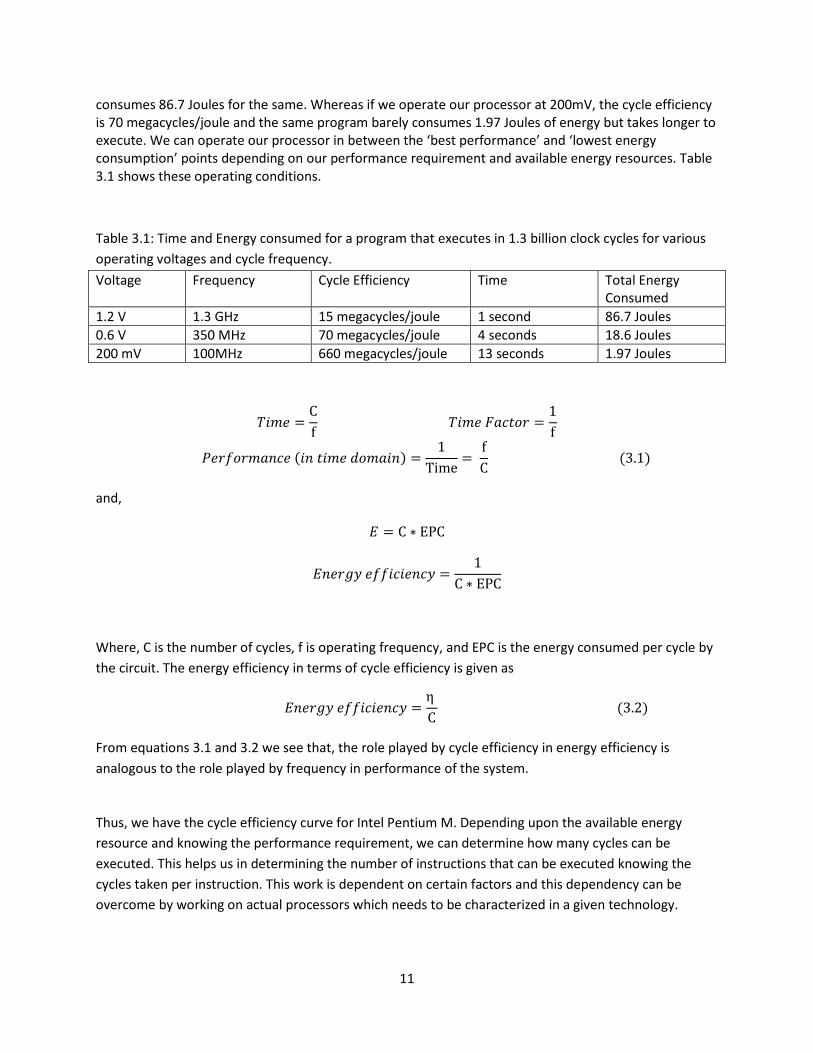
consumes 86.7 Joules for the same. Whereas if we operate our processor at 200mV, the cycle efficiency is 70 megacycles/joule and the same program barely consumes 1.97 Joules of energy but takes longer to execute. We can operate our processor in between the ‘best performance’ and ‘lowest energy consumption’ points depending on our performance requirement and available energy resources. Table 3.1 shows these operating conditions.

Table 3.1: Time and Energy consumed for a program that executes in 1.3 billion clock cycles for various operating voltages and cycle frequency. Voltage Frequency Cycle Efficiency Time Total Energy

Consumed 1.2 V 1.3 GHz 15 megacycles/joule 1 second 86.7 Joules 0.6 V 350 MHz 70 megacycles/joule 4 seconds 18.6 Joules 200 mV 100MHz 660 megacycles/joule 13 seconds 1.97 Joules

𝑇𝑖𝑚𝑒 =Cf

𝑇𝑖𝑚𝑒 𝐹𝑎𝑐𝑡𝑜𝑟 =1f

𝑃𝑒𝑟𝑓𝑜𝑟𝑚𝑎𝑛𝑐𝑒 (𝑖𝑛 𝑡𝑖𝑚𝑒 𝑑𝑜𝑚𝑎𝑖𝑛) =1

Time=

fC

(3.1)

and,

𝐸 = C ∗ EPC

𝐸𝑛𝑒𝑟𝑔𝑦 𝑒𝑓𝑓𝑖𝑐𝑖𝑒𝑛𝑐𝑦 =1

C ∗ EPC

Where, C is the number of cycles, f is operating frequency, and EPC is the energy consumed per cycle by the circuit. The energy efficiency in terms of cycle efficiency is given as

𝐸𝑛𝑒𝑟𝑔𝑦 𝑒𝑓𝑓𝑖𝑐𝑖𝑒𝑛𝑐𝑦 =η C

(3.2)

From equations 3.1 and 3.2 we see that, the role played by cycle efficiency in energy efficiency is analogous to the role played by frequency in performance of the system.

Thus, we have the cycle efficiency curve for Intel Pentium M. Depending upon the available energy resource and knowing the performance requirement, we can determine how many cycles can be executed. This helps us in determining the number of instructions that can be executed knowing the cycles taken per instruction. This work is dependent on certain factors and this dependency can be overcome by working on actual processors which needs to be characterized in a given technology.

12

Chapter 4

Limitations

This work uses power values obtained by running custom microbenchmarks to generate activity in the circuit. Power dissipated by a processor varies with the benchmark program used. Thus the power values have benchmark program dependency. Though our predicted trend holds to be true, the values remain benchmark dependent.

The polynomial equations that we get for the curve for 16 bit adder can be termed as ‘almost perfect estimation’ or curve fitting. So the curve that we get for our Pentium processor has dependencies on curve fitting techniques and trend line formulation.

13

Chapter 5

Conclusion and Future Work

We can have the RTL description of the processor under scrutiny and run standard benchmark programs to get power values and plot the accurate curve. The maximum operating frequency can be decided by extracting the critical path of the given processor. Thus we can change the supply voltage and operating frequency of the processor and have several runs of the benchmark programs.

If the above described technique is ran using various benchmark programs and the values are averaged, the dependency of the power values on the benchmark programs can be reduced to some extent.

We used the existing work done in 90nm technology using the PTM CMOS Model. The same work can be done using other techniques. For example we can use the alpha power law model for MOSFETS to get the delay and the current and then characterize the processor.

14

References

[1] Synopsys, Inc., “HSPICE User Guide: Simulation and Analysis,” www.synopsys.com. [2] http://ark.intel.com/search/advanced?FamilyText=Intel%C2%AE%20Pentium%C2%AE%20Mobile%2

0Processor, accessed on October 10, 2012. [3] Intel Corporation, ”Intel® Pentium® M Processor Datasheet,” download.intel.com/support/

processors/mobile/pm/sb/25261203.pdf.

[4] R. I. Bahar, G. Albera and S. Manne,”Power and Performance Tradeoffs Using Various Caching Strategies,” In Proceedings of the International Symposium on Low Power Electronics and Design, 1998, pp. 64-69.

[5] D. Blaauw,” Power Management Issues in High Performance Processor Design,” In Proceedings of the IEEE Alessandro Volta Memorial Workshop Low-Power Design,” 4-5 Mar., 1999.

[6] D. Brooks, V. Tiwari and M. Martonosi, “Wattch: A Framework for Architectural-Level Power Analysis and Optimizations,” Proceedings of the 27th International Symposium on Computer Architecture (ISCA), June 2000, pp. 83-94.

[7] L. T. Clark, F. Ricci and W. E. Brown,”Dynamic Voltage Scaling With the XScale Embedded Microprocessor,” In Proc. Adaptive Techniques for Dynamic Processor Optimization, 2008, pp. 123-143.

[8] R. Dreslinski, M. Wiekowski, D. Blaauw, D. Slyvester and T. Mudge, ”Near-Threshold Computing:

Reclaiming Moore’s Law Through Energy Efficient Integrated Circuits,” In Proceedings of the IEEE in vol. 98, no. 2, pp. 253-266, Feb. 2010.

[9] D. Folegnani and A. Gonzalez,” Reducing Power Consumption of The Issue Logic,” In Proceedings

2000 Workshop on Complexity Effective Design (WCED) at ISCA 2000, June 2000. [10] R. Gonzalez and M. Horowitz,” Energy Dissipation In General Purpose Microprocessors,” In IEEE

Journal of Solid-State Circuits, Vol. 31, No. 9, Sept. 1996, pp. 1277–1284. [11] H. Hanson, K. Rajamani, S. Keckler, F. Rawson, S. Ghiasi, J. Rubio, “Thermal Response to DVFS:

Analysis with an Intel Pentium M,” In Proceedings of International Symposium on Low Power Electronics and Design, August 27–29, 2007, Portland, Oregon, pp. 219-224.

15

[12] S. Hanson, B. Zhai, M. Seok, B. Cline, K. Zhou, M. Singhal, M. Minuth, J. Olson, L. Nazhandali, T. Austin, D. Sylvester, and D. Blaauw, “Performance And Variability Optimization Strategies In A Sub-200 mv, 3.5 pj/Inst, 11 nw Subthreshold Processor,” In IEEE Symposium on VLSI Circuits, 2007, pp. 152-153.

[13] V. Hanumaiah, S. Vrudhula, and K. S. Chatha, “Performance Optimal Online DVFS and Task

Migration Techniques For Thermally Constrained Multi-Core Processors,” IEEE Transactions on Computer-Aided Design, vol. 30, no. 11, November 2011, pp. 1677–1690.

[14] M. Hicks,” Energy Efficient Branch Prediction” in Doctor of Philosophy thesis, University of

Hertfordshire, Dec. 2007.

[15] R. Joseph and M. Martonosi,” Runtime Power Estimation in High Performance Microprocessors,” in Proceedings of International Symposium on Low Power Electronics and Design, August 6-7, 2001, Huntington Beach, California, pp. 135-140.

[16] K. Kim, “Ultra Low Power CMOS Design” in Doctor of Philosophy’s dissertation, Auburn University,

Dept. of ECE, Auburn, Alabama, May 2011. [17] K. Kim and V. D. Agrawal, “Ultra Low Energy CMOS Logic Using Below-Threshold Dual-Voltage

Supply,” Journal of Low Power Electronics, vol. 7, no. 4, Dec. 2011, pp. 460-470.

[18] K. Kim and V. D. Agrawal, “Minimum Energy CMOS Design with Dual Subthreshold Supply and Multiple Logic-Level Gates,” Proc. International Symp. Quality Electronic Design, 2011, pp. 689-694.

[19] K. Kim and V. D. Agrawal, “Dual Voltage Design for Minimum Energy using Gate Slack,” Proc. International Conf. on Industrial Technology, 2011, pp. 419-424.

[20] K. Kim and V. D. Agrawal, “True Minimum Energy Design Using Dual Below-Threshold Supply Voltages,” Proc. 24th International Conf. on VLSI Design, Jan. 2011, pp. 292-297-424.

[21] W. Kim, M. S. Gupta, G. Wei and D. Brooks, “System Level Analysis Of Fast, Per-Core DVFS Using On-

Chip Switching Regulators,” In Proceedings of the International Symposium on High Performance Computer Architecture, 2008, pp. 123-134.

[22] M. Kulkarni,” A Reduced Constraint Set Linear Program for Low Power Design of Digital Circuits,” Master’s thesis, Auburn University, Dept. of ECE, Auburn, Alabama, Dec 2010

[23] M. Kulkarni and V. D. Agrawal, “A Tutorial on Battery Simulation - Matching Power Source to

Electronic System,” In Proceedings of 14th IEEE VLSI Design and Test Symposium, July 2010. [24] M. Kulkarni and V. D. Agrawal, “Energy Source Lifetime Optimization for a Digital System through

Power Management,” in Proceedings of 43rd IEEE Southeastern Symposium on System Theory, Mar. 2011, pp. 75–80.

[25] J. B. Kuo and J. H. Lou, Low-Voltage CMOS VLSI Circuits, John Wiley, New York, 1999.

16

[26] D. J. Lilja, “Measuring Computer Performance: A Practitioner’s Guide”, Cambridge University Press, New York, NY, 2000.

[27] A. J. Martin, M. Nystrom and P. L. Penzes, “ET2: A Metric for Time and Energy Efficiency of

Computation,” In Power Aware Computing, Kluwer Academic Publishers, Norwell, MA, 2002, pp.293-315.

[28] V. G. Oklobdzija, V. M. Stojanovic, D. M. Markovic and N. Nedovic, “Digital System Clocking: High Performance and Low-Power Aspects,” New York : IEEE ; Hoboken, N.J. : Wiley-Interscience , 2005.

[29] D. Ortiz and N. Santiago, “High-Level Optimization for Low Power Consumption on Microprocessor-Based Systems,” In Proc. 50th Midwest Symposium on Circuits and Systems, 5-8 Aug. 2007, pp. 1265-1268.

[30] V. Paliouras, J. Vounckx and D. Verkest, “Power Consumption Characterization of the Texas Instruments TMS320VC5510 DSP,” In Proc. 15th International Workshop, PATMOS, Leuven, Belgium, Sept. 21-23, 2005, LNCS 3728, pp. 561-570.

[31] D. A. Patterson and J. L. Hennessy, Computer Organization & Design, the Hardware/Software

Interface, Fourth Edition, San Francisco, California: Morgan Kaufman Publishers, Inc., 2008. [32] G. Qu, N. Kawabe, K. Usami and M. Potkonjak, “Function-Level Power Estimation Methodology for

Microprocessors,” In Proceedings of the Design Automation Conference, June 2000, pp. 810-813. [33] R. Rao and S. Vrudhula, “Efficient Online Computation of Core Speeds to Maximize the Throughput

of Thermally Constrained Multi-core Processors,” In Proceedings of the International Conference on Computer-Aided Design, 2008, pp. 53-542.

[34] T. Sakurai and R. Newton, “Alpha-Power Law MOSFET Model and its Applications to CMOS Inverter

Delay and Other Formulas,” In IEEE Journal of Solid-State Circuits, vol. 25, no. 2, pp. 584-594. [35] M. Seok, S. Hanson, Y. S. Lin, Z. Foo, D. Kim, Y. Lee, N. Liu, D. Sylvester and D. Blaauw, “The Phoenix

Processor: A 30pW Platform for Sensor Applications,” In Proceedings of IEEE Symposium on VLSI Circuits, 2008, pp. 188-189.

[36] D. Shin, S. W. Chung, E.-Y. Chung and N. Chang, “Energy-Optimal Dynamic Thermal Management: Computation and Cooling Power Co- Optimization,” IEEE Transactions on Industrial Informatics, vol. 6, no. 3, pp. 340-351, Aug. 2010.

[37] V. Tiwari, R. Donnely, S. Malik and R. Gonzalez, “Dynamic Power Management for Microprocessors:

A Case Study,” In Proc. I0th International Conference on VLSI Design, Jan. 1997, pp. 185-192. [38] V. Tiwari, S. Malik and A. Wolfe, “Power Analysis of Embedded Software: A First Step Towards

Software Power Minimization,” In IEEE transactions on VLSI Systems, vol. 2, no. 4, pp. 437-445, Dec. 1994.

[39] M. Toburen, T. Conte and M. Reilly, “Instruction Scheduling For Low Power Dissipation In High

Performance Microprocessors,” Technical report, North Carolina State University, May 1998.

17

[40] M. A. Viredaz and D. A. Wallach, “Power Evaluation of Itsy Version 2.3. Technical Note TN 57, Digital

Western Research Laboratory, Oct. 2000. [41] M. Venkatasubramanian, “Energy Efficiency and Process Variation Tolerance of 45nm Bulk and

High-k CMOS Devices,” Master’s thesis, Auburn University, Dept. of ECE, Auburn, Alabama, May 2011.

[42] M. Venkatasubramanian and V. D. Agrawal, “Subthreshold Voltage High-k CMOS Devices Have

Lowest Energy and High Process Tolerance,” Proc. 43rd IEEE Southeastern Symp. System Theory, 2011, pp. 98-103

[43] A. Wang, B. H. Calhoun and A. P. Chandrakasan, “Sub-Threshold Design for Ultra Low-Power Systems, New York: Springer, 2006.

[44] N. H. E. Weste and D. Harris, CMOS VLSI Design, Third Edition, Reading, Massachusetts: Addison-

Wesley, 2005.

[45] S. C. Woo, M. Ohara, E. Torrie, J. P. Singh and A Gupta, “The SPLASH-2 Programs: Characterization and Methodological Considerations,” In Proceedings of 22nd IEEE International Symposium on Computer Architecture, 1995, pp. 24-36.

[46] G. K. Yeap, Practical Low Power Digital VLSI Design,” Boston: Springer, 1998.

[47] B. Zhai, R. Dreslinski, T. Mudge, D. Blaauw and D. Sylvester, “Energy Efficient Near-Threshold Chip Multi-Processing,” In Proceedings of IEEE International Symposium on Low-Power Electronics and Design, 2007, pp. 32–37.

[48] W. Zhao and Y. Cao, “New Generation of Predictive Technology Model for Sub-45nm Early Design

Exploration,“ IEEE Transactions on Electron Devices, vol. 53, no. 11, pp. 2816–2823, 2006.

[49] V. Zyuban and P. Kogge, “Optimization of High-Performance Superscalar Architectures for Energy Efficiency,” In Proceedings of the 2000 International Symposium on Low Power Electronics and Design, 2000, pp. 84–89.

[50] V. Zyuban and P. Kogge, “The energy complexity of register files,” In Proceedings of the

International Symposium on Low Power Electronics and Design, 1998, pp. 305-310.