Managing investor and consumer exposure to electricity market … · 2019-10-10 · Managing investor and consumer exposure to electricity market price risks through Feed-in Tariff

Munich Personal RePEc Archive

Managing investor and consumer

exposure to electricity market price risks

through Feed-in Tariff design

Devine, Mel and Farrell, Niall and Lee, William

MACSI, Department of Mathematics and Statistics, University of

Limerick, Limerick, Ireland, Economic and Social Research Institute

and Trinity College, Dublin, Ireland

29 July 2014

Online at https://mpra.ub.uni-muenchen.de/59208/

MPRA Paper No. 59208, posted 15 Oct 2014 12:03 UTC

Managing investor and consumer exposure to electricity market

price risks through Feed-in Tariff design

Mel Devinea,∗, Niall Farrellb,c, William Leea

aMACSI, Department of Mathematics and Statistics, University of Limerick, Limerick, IrelandbEconomic and Social Research Institute, Whitaker Square, Sir John Rogerson’s Quay, Dublin, Ireland

cDepartment of Economics, Trinity College, Dublin, Ireland

Abstract

Feed-in Tariffs (FiTs) incentivise the deployment of renewable energy technologies by subsidising

remuneration and transferring market price risk from investors, through policymakers, to a counter-

party. This counterparty is often the electricity consumer. Different FiT structures exist, with each

transferring market price risk to varying degrees. Explicit consideration of policymaker/consumer

risk burden has not been incorporated in FiT analyses to date. Using Stackelberg game theory

and option pricing, we define FiT policies that efficiently divide market price risk, conditional

on risk preferences and market conditions. We find that commonly employed flat-rate FiTs are

optimal when policymaker risk aversion is extremely low whilst constant premium policies are

optimal when investor risk aversion is extremely low. This suggests that if investors are consid-

erably risk averse, the additional remuneration offered to incentivise deployment under a constant

premium regime may be sub-optimal. Similarly, flat-rate FiTs are sub-optimal if policymakers are

considerably risk averse. When both policymakers and investors are considerably risk averse, an

intermediate division of risk is optimal. We find that investor preferences are more influential than

those of the policymaker when degrees of risk aversion are of a similar magnitude. Efficient divi-

sion of risk is of increasing importance as renewables comprise a greater share of total electricity

cost. Different divisions of market price risk may thus be optimal at different stages of renewables

deployment. Flexibility in FiT legislation may be required to accommodate this.

Keywords: Renewable Energy, Feed-in Tariff, Option Pricing, Renewable Support Schemes,

Market Price Risk

∗Corresponding author: [email protected] +353 (0)61 234 794

Email addresses: [email protected] (Mel Devine), [email protected] (Niall Farrell),

[email protected] (William Lee)

1

1. Introduction

The intermittent nature of many renewable energy sources combine with uncertain market

prices to make renewable energy investment an inherently risky venture. Feed-in Tariffs (FiTs)

guarantee a set payment per unit of electricity generated and thus limit investors’ exposure to low

market prices to a greater extent than alternate mechanisms (Burer and Wustenhagen, 2009; Fagiani

et al., 2013; Haas et al., 2011; IEA and OECD, 2008; Ragwitz et al., 2007). Although theoretically

less efficient than quantity-based schemes (Ringel, 2006), FiTs have become a preferred policy

mechanism for many jurisdictions as the reduced exposure to market price risk has incentivised

greater deployment of renewable technologies (Menanteau et al., 2003; Haas et al., 2011).

FiTs do not eliminate market price risk but rather transfer this risk to a counterparty. This coun-

terparty bears the risk of additional policy cost if wholesale prices are less than the FiT guarantee.

Often, a policymaker incurs this aggregate risk in the first instance, which is then transferred to

electricity consumers through additional charges on consumption (Farrell and Lyons, 2014; Gross

et al., 2010). Different FiT designs apportion this risk in different ways (Couture and Gagnon,

2010; Kim and Lee, 2012), with zero, partial or full transfer of market price risk possible (Farrell

et al., 2013). Although the literature has acknowledged that appropriate risk transfer is central

to successful renewables policy (Klessmann et al., 2013), the optimal division of risk has not

been analysed. The literature to date has concentrated on accommodating investor attitudes to

risk (Burer and Wustenhagen, 2009; Butler and Neuhoff, 2008; Kitzing, 2014; Falconett and Na-

gasaka, 2010; Dong, 2012; Menanteau et al., 2003; Ragwitz et al., 2007; Ringel, 2006). These

analyses have discussed policy cost in terms of expected values but have not addressed policy-

maker/consumer preferences to cost uncertainty when deciding on a policy regime. These factors

are of increasing importance in academic and policy debate as the magnitude of consumer costs are

growing with deployment (Klessmann et al., 2013; Leepa and Unfried, 2013; Loreck et al., 2012).

Market developments may also influence this importance. The proliferation of low-cost unconven-

tional gas may have a depressing effect on fossil fuel prices (Energy Information Administration,

2012; Logan et al., 2013). This may potentially increase the relative cost of renewables (Rauch,

2013) and add to existing risks of an increase in policy cost.

To correctly identify the optimal degree of policy intervention in renewables deployment, a

characterisation of investors’ and policymaker’s/consumers’ attitude to market, regulatory and pol-

icy risks, and their reactions in different contexts, is required (Ekins, 2004; Gross et al., 2010).

Abbreviations: CARA: Constant Absolute Risk Aversion; CE: Certainty Equivalent; CfD: Contract for Differ-

ence; CRRA: Constant Relative Risk Aversion; EMV: Expected Money Value; FiT: Feed-in Tariff; IEA: International

Energy Agency; MW: Megawatt; OECD: Organisation for Economic Cooperation and Development; O & M: Op-

erations & Maintenance; REFIT: Renewable Energy Feed-in Tariff; ROC: Renewables Obligation Certificate; SEM:

Single Electricity Market; VWAP: Volume-Weighted Average Price

2

This paper addresses this gap, contributing a framework to characterise both investor and policy-

maker/consumer exposure to risk, where one can identify the market conditions and attitudes under

which a given degree of policy intervention is optimal. Indeed, optimal division of risk between

investors and policymakers/consumers is analogous to the division of risk central to the design of

insurance contracts (Raviv, 1979). This paper presents a framework to divide risk in a similar way

and is structured as follows. The following section will give a literature review. Section 3 will

outline the economic problem and methodology employed. Section 4 presents the results whilst

Section 5 offers a sensitivity analysis with respect to market parameters and investor/policymaker

attitudes to risk. Finally, Section 6 offers a discussion and conclusion.

2. Literature Review and Motivation

Identifying the optimal division of market price risk brings together literature focussing on in-

vestment incentives and consumer policy cost. Much analysis from an investor’s perspective has

compared FiTs with alternate mechanisms (Dong, 2012; Fagiani et al., 2013; Menanteau et al.,

2003; Ragwitz et al., 2007; Ringel, 2006). FiTs have led to greater deployment than alternatives as

investor exposure to market price risk is lower (Burer and Wustenhagen, 2009; Butler and Neuhoff,

2008; Kitzing, 2014; Falconett and Nagasaka, 2010). Indeed, exposure and attitude to risk is a

key determinant in the superior effectiveness of FiT regimes. Comparing FiTs to quantity-based

policies, Fagiani et al. (2013), Kitzing et al. (2012) and Kitzing (2014) have emphasised the impor-

tance of incorporating market price risk when deciding on a particular policy design, whilst Dinica

(2006) state that the relationship between risk and profitability is key to encouraging investment.

Fewer studies have focussed on how different FiT structures affect investment. Couture and

Gagnon (2010) offer a descriptive comparison of risk exposure under different FiT designs. Kim

and Lee (2012) have analysed FiT payout structures to incentivise Solar PV deployment. Kim

and Lee (2012) incorporate network effects and the propensity to adopt household-based solar

PV. However, they do not evaluate how different attidues to market price risk may affect results.

Doherty and O’Malley (2011) also focus on investors when analysing the efficiency of Ireland’s

FiT design. Although they suggest that the current Irish FiT over-remunerates investors, they do

not compare FiT choice amongst efficiently specified options, nor do they consider consumer and

investor attitidues to market price risk. Farrell et al. (2013) provide a model with which different

FiT regimes may be efficiently defined using option pricing theory. For each design, cost and

remuneration are equal in expectation. However, the balance of certain/uncertain policy cost and

investor remuneration varies between policy options. Farrell et al. (2013) discuss the concept of

risk-sharing when choosing between designs. They do not quantify these preferences nor do they

consider the quantified sensitivity of FiT choice to changes in these preferences.

3

Although managing investor risk exposure has been found to be of great importance for opti-

mal energy policy, less attention has been given to managing policymaker/consumer risk exposure.

However, a body of literature exists to analyse trends in policymaker/consumer cost. Leepa and

Unfried (2013) discuss the impacts of overdeployment and how this may result in excessive con-

sumer cost. Low market prices presents a similar risk of excessive consumer cost. Indeed, a greater

penetration of renewables coupled with lower than expected fossil fuel cost has resulted in greater

subsidies in recent years (Bryant, 2013; Chawla and Pollitt, 2013; DW, 2013; Farrell and Lyons,

2014; Loreck et al., 2012) with potential for this trend to continue (Batlle, 2011; Chawla and Pol-

litt, 2013; Devitt and Malaguzzi Valeri, 2011; Fagiani et al., 2013; Klessmann et al., 2013; Leepa

and Unfried, 2013; Loreck et al., 2012). One can see that increasing policy cost is a consistent

trend, with uncertainty regarding the extent of future policy cost (Devitt and Malaguzzi Valeri,

2011; Klessmann et al., 2013). Given that the setting of a FiT policy is carried out in a prospective

manner, where future costs are uncertain, the incorporation of consumer burden and attitudes to

risk of excessive policy cost is an important consideration.

Thus, it is important to correctly manage both investor and policymaker exposure to market

price risk when designing renewables policy. Discussed in Section 1, such management involves

balancing a trade-off: removing one degree of market price risk from the investor requires the

policymaker to bear an additional degree of risk. Whilst analyses such as that of Kitzing (2014)

and Leepa and Unfried (2013) have considered policy cost under different mechanisms, identifying

the optimal point in this trade-off and efficiently managing policymaker exposure to an unexpected

increase in future policy cost has not been considered. Such efficient division is quite common

in other contexts. Raviv (1979) show that an optimal insurance contract may be designed by first

identifying the insured’s optimal level of coverage as a function of the insurance premium and

then identifying the optimal premium from the insurer’s perspective. Mahul (2001) apply a similar

framework to identify how weather-dependent production may insure against climate risks, whilst

Ma and McGuire (1997) model the design of optimal health insurance contracts.

With regard to FiT policy, analyses to date have compared broad policy specifications (e.g.

fixed premium vs. fixed price) rather than a detailed division of market price risk. Such policy

structures may not allow for the optimal division of risk to be identified. However, Farrell et al.

(2013) have discussed how intermediate divisions of market price risk may be specified. Applying

such a modelling framework allows for the optimal point illustrated in this trade-off to be identified.

3. Materials and Methods

FiTs transfer risk from investors, through policymakers, to consumers. To aid the discussion

that follows, we refer to policymaker burden alone. However, this may be interpreted as a collective

term for the total burden incurred by all consumers. The methodology of this paper comprises

4

three primary steps. First, we model electricity market prices. Second, we specify efficient FiT

specifications which allow for investor remuneration/policy cost to be identified. Third, these

cost/remuneration calculations are used alongside a model of risk averse investment to determine

an optimal FiT design conditional on risk preferences. This methodology is applied to an Irish case

study with data obtained from the literature. These steps will now be outlined in turn.

3.1. Market Prices

The market price, St, received by the renewable investor varies by jurisdiction. For the purpose

of this analysis, we choose an Irish case study and thus consider annual Volume Weighted Aver-

age Prices (VWAP) Farrell et al. (2013). This is the annual average electricity price weighted by

the volume of electricity generated through renewable sources and is used in certain jurisdictions

such as Ireland to calculate wind remuneration (Doherty and O’Malley, 2011; Farrell et al., 2013).

Much literature to date has modelled annual market price processes using a Geometric Brownian

(GBM) (e.g. Yang and Blyth, 2007; Heydari et al., 2012; Zhu, 2012) and we follow this precedent.

Following Farrell et al. (2013), Equations (1) and (2) show that changes in the Q of renewables

installed affect the rate of growth in VWAP. In this way, any changes in prices due to the level of de-

ployment are endogenous to the assumed price process and thus the investment decision. VWAPs

are modeled this way because the ‘merit order effect’ of certain renewables with no marginal cost

(e.g. wind, wave solar; Sensfuß et al., 2008) will result in lower rates of market price growth as the

quantity Q of installed capacity increases.

dS = µ(Q)Sdt+ σSdω, (1)

where

µ(Q) = µ+ ηe−κQ, (2)

and dω represents the increment of the Wiener process.

3.2. Feed-in Tariff Prices

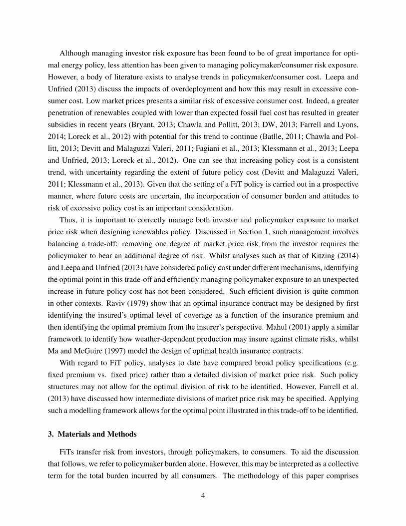
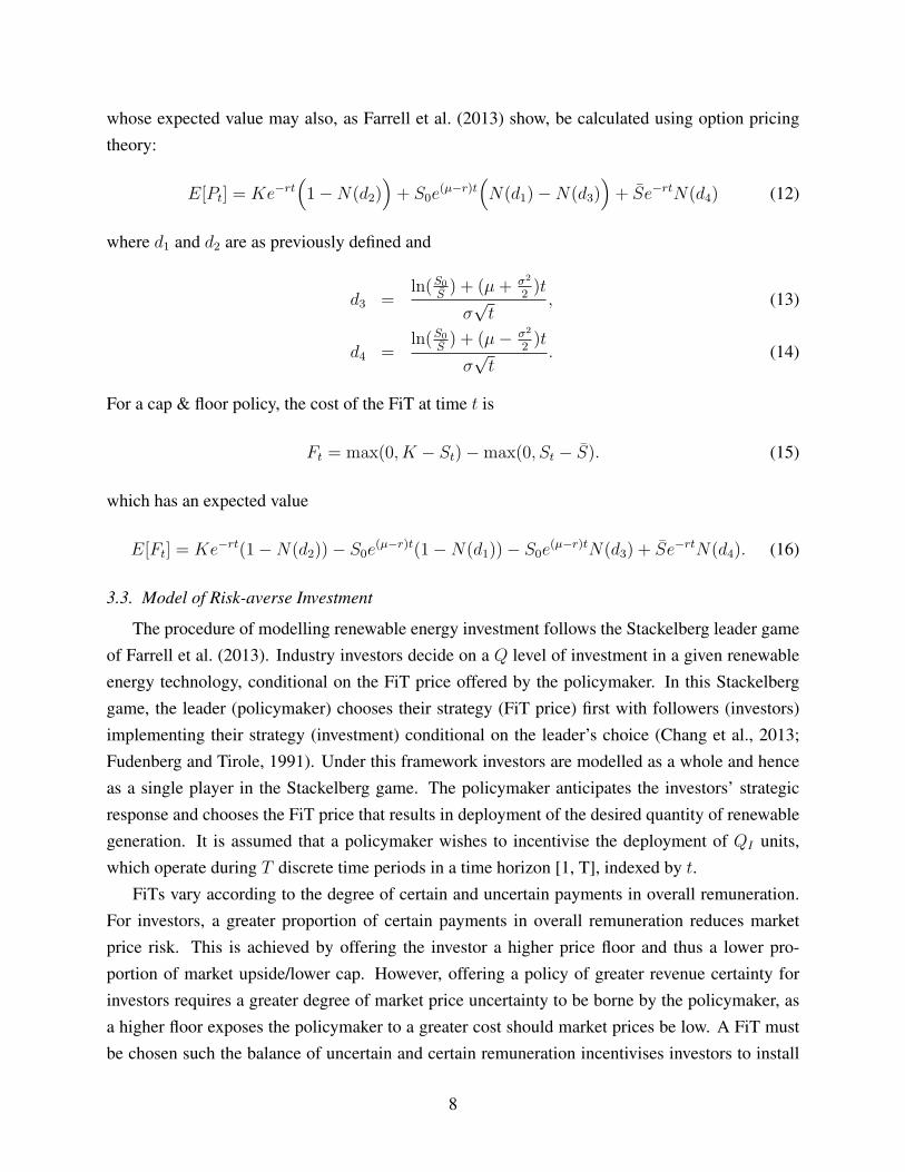
Once market prices are specified, we must specify efficient feed-in tariff prices. These are de-

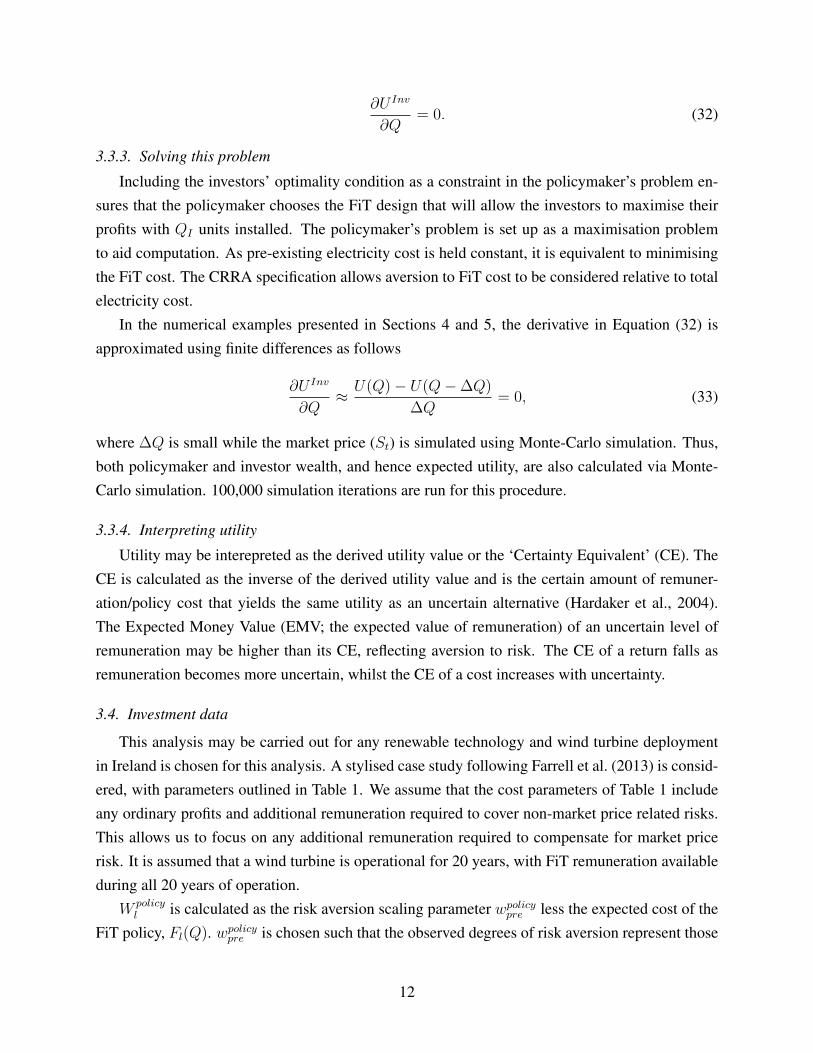
rived using the methodology proposed by Farrell et al. (2013). Illustrated in Figure 1, Different FiT

designs transfer market price risk in different ways. Potential designs include a constant premium,

where investors receive the market price and a constant premium during each trading period; a

price floor with market upside shared between investors and policymakers; or a cap & floor policy.

A cap & floor places upper and lower bounds on the market price received by investors, whilst

a shared upside offers investors a guaranteed price floor and a share of all market upside. A con-

stant premium offers investors the market price and a constant premium at all times of generation.

Farrell et al. (2013) show how each of these FiTs may be efficiently specified using option pricing

5

Pric

e

Time

FiT Remuneration

Market Price P

ric

e

Time

Market Price

Price Floor

FiT Remuneration

Pric

e

Time

Market Price Price Cap/Floor FiT Remuneration

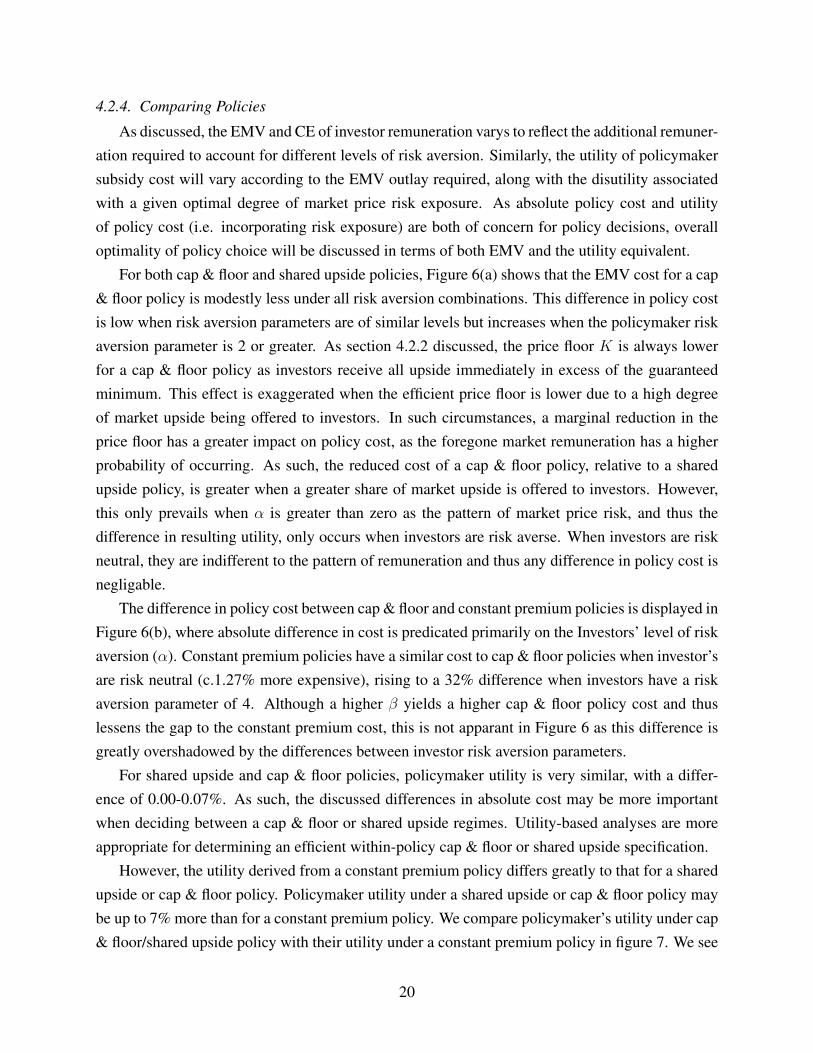
Figure 1: Payment structures: (left) constant premium, (middle) shared upside, (right) cap & floor.

theory. Certain elements of remuneration (i.e. caps or floors) are defined such that the expected

value of uncertain market remuneration is taken into account. As such, a price floor would be

lower than if no market upside were offered to investors and thus total remuneration (i.e. price

floor remuneration + market upside) as opposed to the price floor alone, is sufficient to incentivise

investment. This specification results in an inverse relationship between the efficient price floor

and the degree of market ‘upside’ offered to investors. Should no market ‘upside’ be shared with

investors, efficient price floors are highest, with both shared upside and cap & floor policies con-

verging on a flat-rate price for investors. As a greater share of market upside is offered to investors,

the efficient price floor falls to take into account of the value of the market upside. This continues

until all market ‘upside’ is available to investors and both shared upside and cap & floor policies

converge on a price floor regime. Policymakers incur a subsidisiation cost for every trading period

when market prices are less than pre-specified price floors and receive a benefit if they exceed a

price cap. For a shared upside regime, policymakers receive a predefined share of the market up-

side in excess of the price floor. The procedure of efficient FiT specification developed by Farrell

et al. (2013) is adopted for this study and will now be summarised.

3.2.1. Constant Premium

For a constant premium tariff, the discounted price received by the investor during time t (Pt)

is the discounted value of the premium, X , added to the discounted value of market remuneration:

Pt = e−rt(X + St), (3)

which has a expected value

E[Pt] = Xe−rt + S0e(µ−r)t. (4)

6

The cost for the policymaker, at time t, is constant at X .

3.2.2. Shared Upside

The expected value of remuneration under a shared upside policy comprises two constituent

elements; a minimum price guarantee and a portion of market upside. Specifying the expected

value of remuneration under this policy type must incorporate the expected value of both elements.

This FiT structure resembles a European put option, where the investor has the right, but not the

obligation to sell at time t at a given price (i.e., price floor K), but may also sell at the market price

St should it exceed this floor. Farrell et al. (2013) augment option pricing theory to value Pt under

a shared upside policy, with the discounted price at time t denoted as:

Pt = e−rt(K + θ(max(St −K, 0))), (5)

which has an expected value

E[Pt] = Ke−rt(1− θN(d2)) + θS0e(µ−r)tN(d1), (6)

where N(.) represents the cumulative distribution function of the standard normal distribution

while

d1 =ln(S0

K) + (µ+ σ2

2)t

σ√t

, (7)

d2 =ln(S0

K) + (µ− σ2

2)t

σ√t

. (8)

Discounted policy cost under a shared upside regime is

Ft = e−rt(max(0, K − St)− (1− θ)max(0, St −K)). (9)

whose expected value may also be calculated using option pricing theory, as follows:

E[Ft] = Ke−rt − S0e(µ−r)t + θ

(

S0e(µ−r)tN(d1)−Ke−rtN(d2)

)

. (10)

3.2.3. Cap & Floor

A cap & floor policy is also like a put option, where investors have the right to sell at a price

floor, but may sell at the market price should it exceed the floor. However, should the price exceed

the cap, remuneration is equal to the cap and no more. The price Pt under this policy design is:

Pt = e−rt(K +max(St −K), 0)−max(St − S, 0)) (11)

7

whose expected value may also, as Farrell et al. (2013) show, be calculated using option pricing

theory:

E[Pt] = Ke−rt(

1−N(d2))

+ S0e(µ−r)t

(

N(d1)−N(d3))

+ Se−rtN(d4) (12)

where d1 and d2 are as previously defined and

d3 =ln(S0

S) + (µ+ σ2

2)t

σ√t

, (13)

d4 =ln(S0

S) + (µ− σ2

2)t

σ√t

. (14)

For a cap & floor policy, the cost of the FiT at time t is

Ft = max(0, K − St)−max(0, St − S). (15)

which has an expected value

E[Ft] = Ke−rt(1−N(d2))− S0e(µ−r)t(1−N(d1))− S0e

(µ−r)tN(d3) + Se−rtN(d4). (16)

3.3. Model of Risk-averse Investment

The procedure of modelling renewable energy investment follows the Stackelberg leader game

of Farrell et al. (2013). Industry investors decide on a Q level of investment in a given renewable

energy technology, conditional on the FiT price offered by the policymaker. In this Stackelberg

game, the leader (policymaker) chooses their strategy (FiT price) first with followers (investors)

implementing their strategy (investment) conditional on the leader’s choice (Chang et al., 2013;

Fudenberg and Tirole, 1991). Under this framework investors are modelled as a whole and hence

as a single player in the Stackelberg game. The policymaker anticipates the investors’ strategic

response and chooses the FiT price that results in deployment of the desired quantity of renewable

generation. It is assumed that a policymaker wishes to incentivise the deployment of QI units,

which operate during T discrete time periods in a time horizon [1, T], indexed by t.

FiTs vary according to the degree of certain and uncertain payments in overall remuneration.

For investors, a greater proportion of certain payments in overall remuneration reduces market

price risk. This is achieved by offering the investor a higher price floor and thus a lower pro-

portion of market upside/lower cap. However, offering a policy of greater revenue certainty for

investors requires a greater degree of market price uncertainty to be borne by the policymaker, as

a higher floor exposes the policymaker to a greater cost should market prices be low. A FiT must

be chosen such the balance of uncertain and certain remuneration incentivises investors to install

8

QI units whilst allowing policymakers to minimise the welfare loss associated with policy cost

and exposure to market price risk. Incorporating aversion to market price risk when evaluating

cost/remuneration may be incorporated into the decision-making process through the use of a util-

ity function. Under the axioms of a von Neumann-Morgenstern utility function a decision-maker

is risk-averse, rational and will act to maximise expected utility (von Neumann and Morgenstern,

1947). A number of utility function specifications exist, each of which may be potentially chosen.

A Constant Absolute Risk Aversion (CARA) utility function has a constant degree of risk aversion

regardless of the absolute level of the outcome variable being analysed (e.g. wealth, consump-

tion, cost). A Constant Relative Risk Aversion (CRRA) utility function is similar however it has a

scaling factor which calibrates the agent’s degree of risk aversion according to a pre-existing level

of the outcome variable (Arrow, 1971; Meyer and Meyer, 2005). For policymakers, the outcome

variable is electricity cost. The literature to date suggests an increasing concern surrounding FiT

costs as they comprise a greater share of total electricity cost (Batlle, 2011; Leepa and Unfried,

2013; Loreck et al., 2012). As such, policymakers may become more averse to FiT cost uncertain-

ties as they comprise a greater proportion of electricity cost. A CRRA functional form captures

this relationship. For investors, wealth is the outcome variable. Much of the literature to date has

employed a CRRA functional form when analysing investment in energy markets and large scale

investments (Chronopoulos et al., 2014; Cotter and Hanly, 2012). Given this precedent and ability

to calibrate CRRA utility functions to a realistic degree of risk aversion, a CRRA functional form

is chosen for this analysis.

3.3.1. Investor Utility

Under a CRRA utility function, utility for the investor and policymaker is comprised of a

scaling parmaeter and profit/cost of deployment. Generally, pre-existing wealth is used for this

scaling parameter. For policymakers and investors in renewable energy, pre-existing wealth may

be difficult to define. To ensure that our results are calibrated to realistic degree of risk aversion, we

choose the scaling parameter such that the resulting rates of risk aversion are deemed reasonable

given the literature. Such flexibility is a further benefit of the CRRA utility function over less

flexible forms such as the CARA functional form.

We model investors in a given market together as one entity (Farrell et al., 2013). The investors’

utility, under scenario l, is modelled using a power law utility function with risk aversion parameter

α ≥ 0:

U Invl =

(

11−α

)

(W Invl )1−α if α 6= 1

ln(W Invl ) if α = 1

(17)

The investors’ outcome variable, wealth (W Invl ) under scenario l, is comprised of the scaling

9

parameter wInvpre and profit from investment, Πl(Q). This profit is uncertain and subject to fluc-

tuations in market prices and thus varies from scenario to scenario. The amount of uncertainty

differs depending on the policy enacted. The investors’ profit is also dependent on Q, the number

of installed units of renewable energy technology. The Investors’ wealth under scenario l is

W Invl = wInv

pre +Πl(Q). (18)

Total industry profit Πl(Q), received during operation from time t = 1 to T , is defined accord-

ing to Equation (19).

Πl(Q) =∑

t

[Pt(Q)G(Q)]− C(Q), (19)

where Pt is the discounted price received during time t, which may be either the market price St1 or

the guaranteed price offered by a given FiT regime. Guaranteed elements of investor remuneration

may be either a price floor (K) a cap (S) or a share of market upside (θ), depending on the FiT

design chosen.

For the installation of Q units, C(Q) is the sum of industry-level capital (A) and operating (O)

costs (including any required return to personnel, capital, etc.), discounted according to a discount

rate r:

C(Q) = AQ+T∑

t=1

e−rtOQ (20)

The amount of electricity generated from renewable sources during time t is G(Q). As with

Farrell et al. (2013) this function is calculated according to the following equation:

G(Q) = b(Q)uvh (21)

where v is operational availability net of maintenance and other such outages, u is the capacity

factor for initial units and h is the number of hours per time period t. The function b is given by

b(Q) = Qmax(1− e−γQ) (22)

where Qmax is the maximum potential Q, whilst γ is a parameter controlling the rate of change.

Equation (22) models capacity by incorporating changes in effective capacity/availability as Q

changes2.

The investors’ objective is to maximise expected utility by choosing a Q level of output:

1While Pt and St are both determined stochastically and hence vary from scenario to scenario, for ease of presen-

tation, the subscript l is ignored for these two variables.2See Farrell et al. (2013) for further discussion on Equations (21) and (22).

10

maxQ

U Inv = maxQ

E[U Invl ], (23)

maxQ

U Inv = maxQ

∫ ∞

0

(

1

1− α

)(

W Invl (Q)

)1−α

Pr(l)dl, (24)

where Pr(l) is the probability associated with scenario l. Assuming concavity, the investors’ utility

function is maximised when∂U Inv

∂Q= 0. (25)

3.3.2. Policymaker Utility

In a similar manner to above, the policymaker’s utility, under scenario l, is modelled using a

power law utility function with risk aversion parameter β ≥ 0:

Upolicyl =

(

11−β

)(

W policyl

)1−β

if β 6= 1

ln(W policyl ) if β = 1

(26)

The policymaker’s outcome variable is total electricity cost, W policyl under scenario l. This is

comprised of the scaling parameter,wpolicypre , less the cost of the chosen FiT design. This is calculated

as follows

W policyl = wpolicy

pre − Fl(Q). (27)

As with the investors’ profits, the cost Fl(Q) is subject to fluctuations in market prices and thus

varies from scenario to scenario whilst also depending on the amount of units of renewable energy

technology installed. This cost is the sum of the difference between the price that the investors

receives Pt and the market price St:

Fl =∑

t

Ft =∑

t

Pt(Q)− St(Q) (28)

The policymaker’s goal is to choose the FiT design that maximises their expected utility whilst

ensuring that investors choose QI units of renewable energy technology as follows:

maxUpolicy = maxE[Upolicyl ], (29)

maxUpolicy = max

∫ ∞

0

(

1

1− β

)(

W policyl

)1−β

Pr(l)dl, (30)

subject to

Q = QI , (31)

11

∂U Inv

∂Q= 0. (32)

3.3.3. Solving this problem

Including the investors’ optimality condition as a constraint in the policymaker’s problem en-

sures that the policymaker chooses the FiT design that will allow the investors to maximise their

profits with QI units installed. The policymaker’s problem is set up as a maximisation problem

to aid computation. As pre-existing electricity cost is held constant, it is equivalent to minimising

the FiT cost. The CRRA specification allows aversion to FiT cost to be considered relative to total

electricity cost.

In the numerical examples presented in Sections 4 and 5, the derivative in Equation (32) is

approximated using finite differences as follows

∂U Inv

∂Q≈ U(Q)− U(Q−∆Q)

∆Q= 0, (33)

where ∆Q is small while the market price (St) is simulated using Monte-Carlo simulation. Thus,

both policymaker and investor wealth, and hence expected utility, are also calculated via Monte-

Carlo simulation. 100,000 simulation iterations are run for this procedure.

3.3.4. Interpreting utility

Utility may be interepreted as the derived utility value or the ‘Certainty Equivalent’ (CE). The

CE is calculated as the inverse of the derived utility value and is the certain amount of remuner-

ation/policy cost that yields the same utility as an uncertain alternative (Hardaker et al., 2004).

The Expected Money Value (EMV; the expected value of remuneration) of an uncertain level of

remuneration may be higher than its CE, reflecting aversion to risk. The CE of a return falls as

remuneration becomes more uncertain, whilst the CE of a cost increases with uncertainty.

3.4. Investment data

This analysis may be carried out for any renewable technology and wind turbine deployment

in Ireland is chosen for this analysis. A stylised case study following Farrell et al. (2013) is consid-

ered, with parameters outlined in Table 1. We assume that the cost parameters of Table 1 include

any ordinary profits and additional remuneration required to cover non-market price related risks.

This allows us to focus on any additional remuneration required to compensate for market price

risk. It is assumed that a wind turbine is operational for 20 years, with FiT remuneration available

during all 20 years of operation.

W policyl is calculated as the risk aversion scaling parameter wpolicy

pre less the expected cost of the

FiT policy, Fl(Q). wpolicypre is chosen such that the observed degrees of risk aversion represent those

12

expected by the literature. Hirst (2002) estimate that hedging wholesale market price risk to pro-

vide a fixed cost for consumers adds 5-10% onto electricity cost. Zhang and Wang (2009) analyse a

number of contracts to provide a hedge against wholesale market fluctuations for consumers, find-

ing that contract prices may range anywhere from 0.38% to 23% of the electricity price, depending

on the portion of the load that is hedged. For fixed price tariffs with a high fixed price, they find

that hedge contracts may range from 0.38-4.12%. This literature analysing electricty price hedging

focuses on hedging all market price risk, not just the FiT cost portion. Given that FiT costs com-

prise a smaller proportion of electricity cost than the total electricity cost that is analysed in these

papers, we take this lower range as being a more representative range of hedge values considered.

We chose this range for our baseline analysis but test senstivity to alternate ranges in Section 5.

Similarly, winvpre is chosen such that investors’ risk aversion is of a range considered realis-

tic.Hern et al. (2013) survey wind investors in the UK and find that switching from a Renewable

Obligation Certificate (ROC) scheme to a FiT through Contracts for Difference (CfD), in essence

a switch from incurring market price risk to incurring no market price risk, results in a 20% reduc-

tion in the expected rate of profitability for onshore wind. This gives a rough benchmark as to the

premium required for incurring market price risk in wind investment. Although providing a suit-

able benchmark, the degree of risk presented to UK investors is slightly different to that in Ireland

and actual premiums in an Irish context may deviate from this benchmark. Indeed, premiums may

vary for each investor. Nevertheless, in the absence of further information, the findings of Hern

et al. (2013) provide a useful calibration point, where baseline findings of ‘high’, ‘expected’ or

‘low’ levels of investor risk aversion may be interpreted relative to this benchmark.

Risk aversion parameters generally range from 0 (risk neutral) to 4 (extremelely risk-averse)

for CRRA utility functions (Anderson and Dillon, 1992). Arrow (1965) assumes that risk aversion

’hovers about 1’. As such, winvpre is assumed to be e18.98bn such that a change from a policy of

constant premium to fixed price requires a c.20% premium on investment when the risk aversion

parameter is 1. If one believes that alternate levels of risk aversion are more appropriate, a wide

range of risk aversion parameters are modelled to capture the optimal investment. We also carry out

a sensitivity analysis with respect to the winvpre parameter to capture further degrees of risk aversion.

Section 4.1 discusses the implications of different risk aversion parameters to aid interpretation

should the reader prefer alternate levels of risk aversion.

4. Results and Discussion

4.1. Risk Aversion

First we present quantified representations of risk aversion to aid interpretation of policy choice

results. Table 2 shows the CE of 20-year discounted policy cost under different levels of risk

aversion (β) for a shared upside policy when θ = 1. When β = 0, the CE is the same as the

13

Table 1: Baseline Simulation parameters

Parameter Value

Capital Cost (Wind, per MW) e1.76ma

Annual Operations & Maintenance Cost 2% of capital costa

Irish Single Electricity Market (SEM) Installation target (QI) 4,630 MWb

Capacity Factor (u) 0.35a

Availability (v) 0.95a

Maximum Q (Qmax) 16 GWc

γ (6.75× 10−5 )b

Generation during t (Gt) 12,501,319 e

Long-run electricity Price Growth (µ) 0.0155a

η 0.01 e

κ 0.001d

Electricity Price Volatility (σ) 0.13a

Initial VWAP (S0) e52.41a

Discount Rate (r) 0.06

winvpre e18.98bne

wpolicypre e38.36bne

Source: a calibrated to Doherty and O’Malley (2011); bcallibrated to Mc Garrigle et al. (2013);c SEAI (2011); dcalibrated to IWEA (2011); e own calculation

expected value of remuneration. One can see that as the risk aversion parameter β grows, the CE

grows also as the policymaker is willing to incur a greater certain policy cost in order to forego a

given level of cost uncertainty. When a β parameter of 1 is in place, the policymaker is willing to

take a certain cost that is 1.36% higher to forego the possibility of incurring extremely high policy

cost. One can see that this threshold increases as the policymaker’s level of risk aversion grows,

with a β value of 4 implying that a policymaker is indifferent between incurring the uncertain

policy cost and a certain payment that is 5.527% greater than the expected value (i.e. β = 0).

Table 2: Certainty equivalent of 20-year discounted policy cost by level of risk aversion (β)

β 0 1 2 3 4

Certainty Equivalent 3.252bn 3.296bn 3.341bn 3.386bn 3.432bn

Increase relative to β = 0 0 1.367% 2.745% 4.132% 5.527%

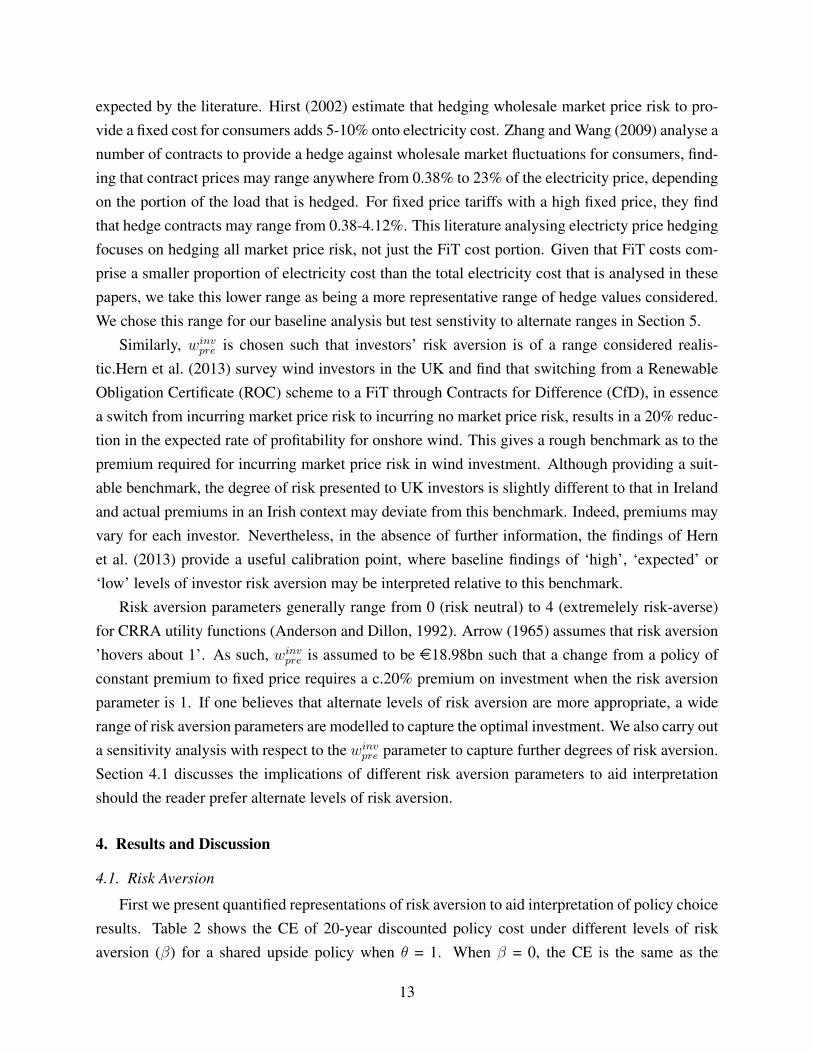
To understand investor risk aversion, Figure 2 compares the change in EMV required by an

investor under different α risk aversion parameters as a result of switching from a fixed price

policy (θ = 0) to varying degrees of shared upside and a constant premium. One can see that when

α = 1, EMV must be c.20% greater for investment under a constant premium. This corresponds

to the added remuneration quoted by Hern et al. (2013) and thus provides a suitable benchmark

14

Figure 2: Quantification of Investor Risk Aversion

0 0.5 1 1.5 2 2.5 3 3.5 40

10

20

30

40

50

60

70%

incr

ease

in E

[NP

V]

α

Constant Premiumθ = 0.5θ = 1

rate of investor risk aversion. One can see that the risk-sharing properties of the shared upside

policies result in a much lower additional level of remuneration than the constant premium regime.

However, EMV is still c.5-10% greater than when θ = 0. These rates of risk aversion are given

greatest attention in this analysis. Section 5 presents results relative to alternate ranges of risk

aversion.

4.2. Optimal policy choice

We identify optimal levels of market price risk division both within and between policy types.

This is first carried out for the discussed baseline scenario, followed by a sensitivity analysis with

respect to the calibrated degree of risk aversion and assumed market price parameters. Quantify-

ing such sensitivity gives insight into what FiT policy designs may be optimal when parameters

differ from our baseline assumptions. The results of Table 2 and Figure 2 may be used to aid

interpretation of risk aversion parameters in the baseline discussion that follows.

4.2.1. Optimal shared upside policy

Figures 3(a) and 3(b) show the optimal price floor (denoted K) and corresponding share of

market upside (θ) for each α and β combination. We find an inverse relationship, predicted by

Farrell et al. (2013), where a larger share of market upside (θ) results in a smaller price floor (K).

Figure 3 shows that the optimal division of market price risk is primarily a function of the

relative balance of risk aversion. If investors have very low level of risk aversion, (≤ 0.25) and

15

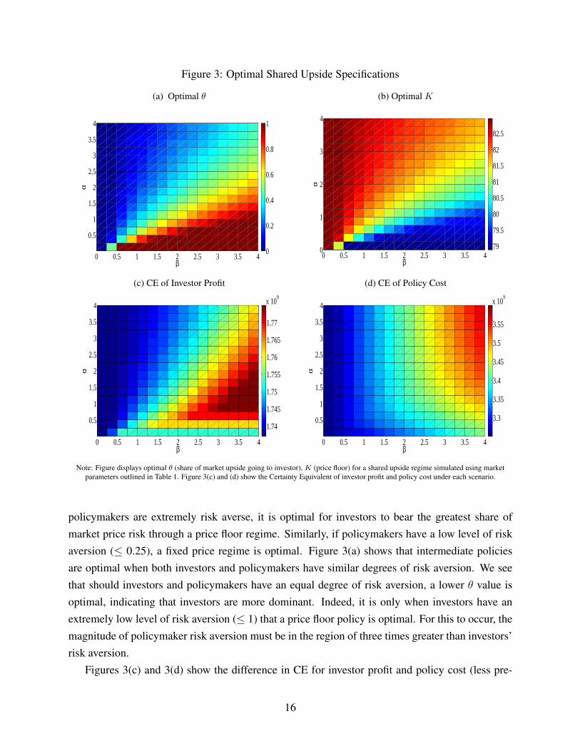
Figure 3: Optimal Shared Upside Specifications

(a) Optimal θ

0 0.5 1 1.5 2 2.5 3 3.5 4

0.5

1

1.5

2

2.5

3

3.5

4

α

β

0

0.2

0.4

0.6

0.8

1

(b) Optimal K

0 0.5 1 1.5 2 2.5 3 3.5 40

1

2

3

4

β

α

79

79.5

80

80.5

81

81.5

82

82.5

(c) CE of Investor Profit

0 0.5 1 1.5 2 2.5 3 3.5 4

0.5

1

1.5

2

2.5

3

3.5

4

α

β

1.74

1.745

1.75

1.755

1.76

1.765

1.77

x 109

(d) CE of Policy Cost

0 0.5 1 1.5 2 2.5 3 3.5 4

0.5

1

1.5

2

2.5

3

3.5

4α

β

3.35

3.45

3.55

3.4

3.5

3.3

x 109

Note: Figure displays optimal θ (share of market upside going to investor), K (price floor) for a shared upside regime simulated using market

parameters outlined in Table 1. Figure 3(c) and (d) show the Certainty Equivalent of investor profit and policy cost under each scenario.

policymakers are extremely risk averse, it is optimal for investors to bear the greatest share of

market price risk through a price floor regime. Similarly, if policymakers have a low level of risk

aversion (≤ 0.25), a fixed price regime is optimal. Figure 3(a) shows that intermediate policies

are optimal when both investors and policymakers have similar degrees of risk aversion. We see

that should investors and policymakers have an equal degree of risk aversion, a lower θ value is

optimal, indicating that investors are more dominant. Indeed, it is only when investors have an

extremely low level of risk aversion (≤ 1) that a price floor policy is optimal. For this to occur, the

magnitude of policymaker risk aversion must be in the region of three times greater than investors’

risk aversion.

Figures 3(c) and 3(d) show the difference in CE for investor profit and policy cost (less pre-

16

existing wealth) to give insight into the additional remuneartion required for the risk borne by each

party under each scenario. Interestingly, we see different patterns for investor and policymaker

risk.

In Figure 3(c) we see that additional investor remuneration to account for price risk is greatest

when policymaker risk aversion is high (about 4) and investor risk aversion is about 1. In such

circumstances, the policymaker’s preferences dominate those of the investor, and a θ close to 1

prevails. This requires investors to incur almost all market price risk. As the optimal θ is higher

than alternate scenarios where α is high, investors require a greater degree of additional remuner-

ation to bear this additional risk. Under this circumstance the policymaker is willing to incur a

considerable additional certain cost to ensure that they minimise their exposure to market price

risk. However, this diagram shows that offering such an additional level of remuneration is only

optimal when policymaker’s level of risk aversion is much greater than investors. The disutility

associated with an increase in additional investor payments shown in Figure 3(c) combines with

the greater disutility associated with increased investor risk aversion to give the pattern of Figure

3(d). Figure 3(d) shows that policymaker disutility grows with both investor and policymaker risk

aversion.

4.2.2. Optimal cap & floor policy

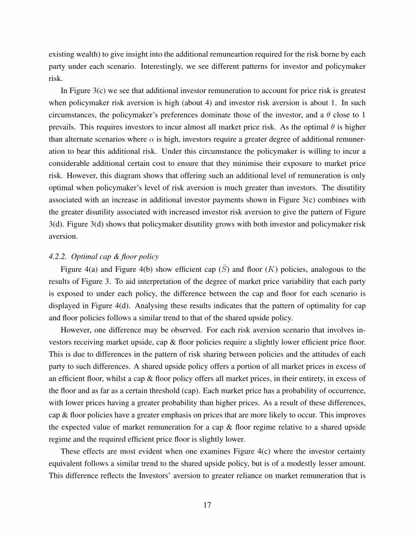
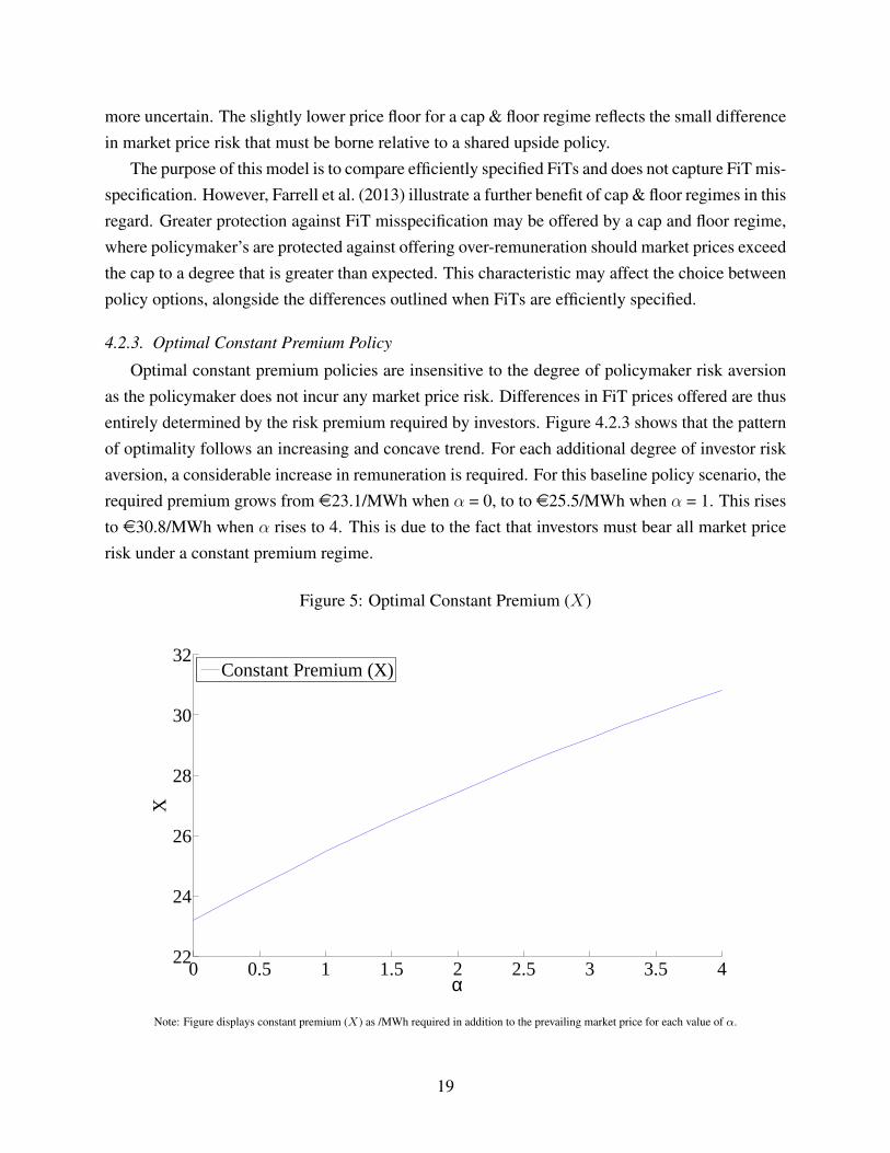
Figure 4(a) and Figure 4(b) show efficient cap (S) and floor (K) policies, analogous to the

results of Figure 3. To aid interpretation of the degree of market price variability that each party

is exposed to under each policy, the difference between the cap and floor for each scenario is

displayed in Figure 4(d). Analysing these results indicates that the pattern of optimality for cap

and floor policies follows a similar trend to that of the shared upside policy.

However, one difference may be observed. For each risk aversion scenario that involves in-

vestors receiving market upside, cap & floor policies require a slightly lower efficient price floor.

This is due to differences in the pattern of risk sharing between policies and the attitudes of each

party to such differences. A shared upside policy offers a portion of all market prices in excess of

an efficient floor, whilst a cap & floor policy offers all market prices, in their entirety, in excess of

the floor and as far as a certain threshold (cap). Each market price has a probability of occurrence,

with lower prices having a greater probability than higher prices. As a result of these differences,

cap & floor policies have a greater emphasis on prices that are more likely to occur. This improves

the expected value of market remuneration for a cap & floor regime relative to a shared upside

regime and the required efficient price floor is slightly lower.

These effects are most evident when one examines Figure 4(c) where the investor certainty

equivalent follows a similar trend to the shared upside policy, but is of a modestly lesser amount.

This difference reflects the Investors’ aversion to greater reliance on market remuneration that is

17

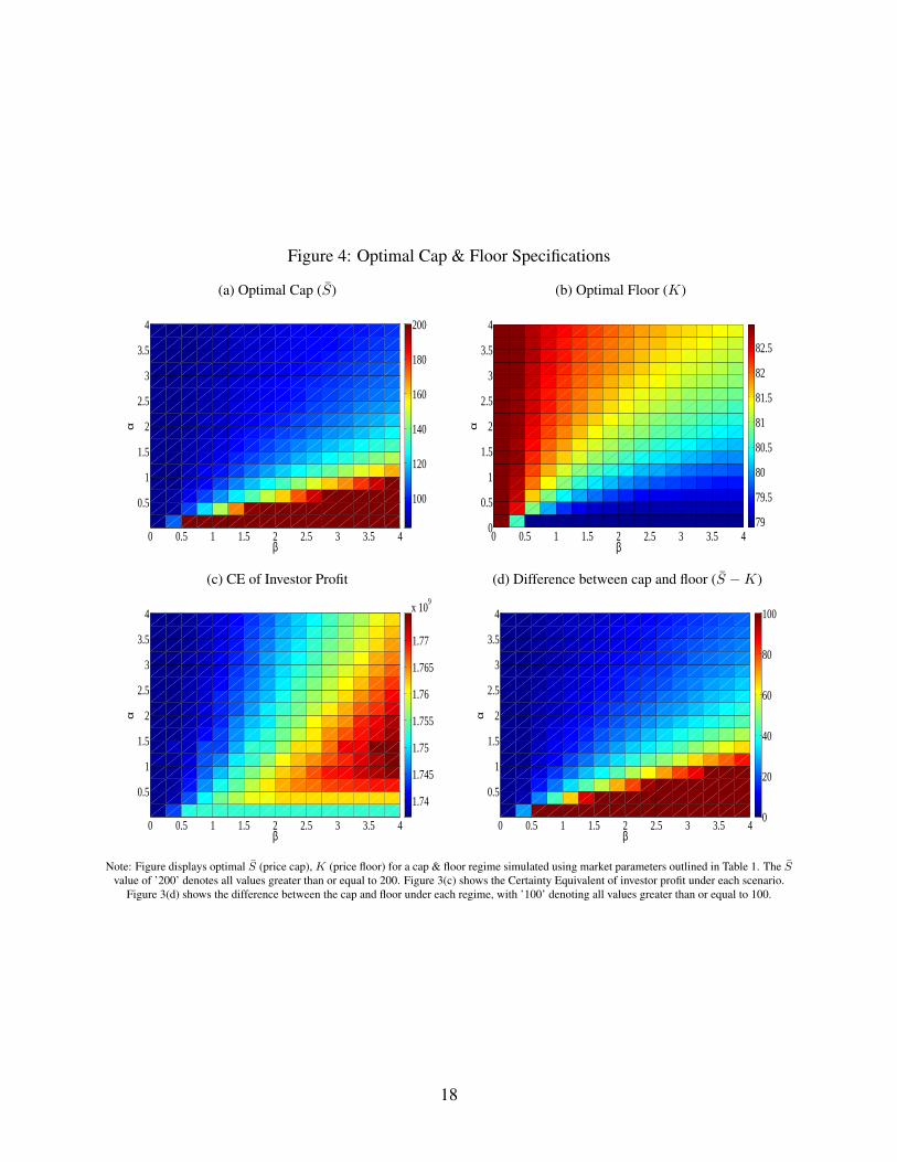
Figure 4: Optimal Cap & Floor Specifications

(a) Optimal Cap (S)

0 0.5 1 1.5 2 2.5 3 3.5 4

0.5

1

1.5

2

2.5

3

3.5

4

β

α

100

120

140

160

180

200

(b) Optimal Floor (K)

0 0.5 1 1.5 2 2.5 3 3.5 40

0.5

1

1.5

2

2.5

3

3.5

4

β

α

79

79.5

80

80.5

81

81.5

82

82.5

(c) CE of Investor Profit

0 0.5 1 1.5 2 2.5 3 3.5 4

0.5

1

1.5

2

2.5

3

3.5

4

β

α

1.74

1.745

1.75

1.755

1.76

1.765

1.77

x 109

(d) Difference between cap and floor (S −K)

0 0.5 1 1.5 2 2.5 3 3.5 4

0.5

1

1.5

2

2.5

3

3.5

4

β

α

0

20

40

60

80

100

Note: Figure displays optimal S (price cap), K (price floor) for a cap & floor regime simulated using market parameters outlined in Table 1. The S

value of ’200’ denotes all values greater than or equal to 200. Figure 3(c) shows the Certainty Equivalent of investor profit under each scenario.

Figure 3(d) shows the difference between the cap and floor under each regime, with ’100’ denoting all values greater than or equal to 100.

18

more uncertain. The slightly lower price floor for a cap & floor regime reflects the small difference

in market price risk that must be borne relative to a shared upside policy.

The purpose of this model is to compare efficiently specified FiTs and does not capture FiT mis-

specification. However, Farrell et al. (2013) illustrate a further benefit of cap & floor regimes in this

regard. Greater protection against FiT misspecification may be offered by a cap and floor regime,

where policymaker’s are protected against offering over-remuneration should market prices exceed

the cap to a degree that is greater than expected. This characteristic may affect the choice between

policy options, alongside the differences outlined when FiTs are efficiently specified.

4.2.3. Optimal Constant Premium Policy

Optimal constant premium policies are insensitive to the degree of policymaker risk aversion

as the policymaker does not incur any market price risk. Differences in FiT prices offered are thus

entirely determined by the risk premium required by investors. Figure 4.2.3 shows that the pattern

of optimality follows an increasing and concave trend. For each additional degree of investor risk

aversion, a considerable increase in remuneration is required. For this baseline policy scenario, the

required premium grows from e23.1/MWh when α = 0, to to e25.5/MWh when α = 1. This rises

to e30.8/MWh when α rises to 4. This is due to the fact that investors must bear all market price

risk under a constant premium regime.

Figure 5: Optimal Constant Premium (X)

0 0.5 1 1.5 2 2.5 3 3.5 422

24

26

28

30

32

X

α

Constant Premium (X)

Note: Figure displays constant premium (X) as /MWh required in addition to the prevailing market price for each value of α.

19

4.2.4. Comparing Policies

As discussed, the EMV and CE of investor remuneration varys to reflect the additional remuner-

ation required to account for different levels of risk aversion. Similarly, the utility of policymaker

subsidy cost will vary according to the EMV outlay required, along with the disutility associated

with a given optimal degree of market price risk exposure. As absolute policy cost and utility

of policy cost (i.e. incorporating risk exposure) are both of concern for policy decisions, overall

optimality of policy choice will be discussed in terms of both EMV and the utility equivalent.

For both cap & floor and shared upside policies, Figure 6(a) shows that the EMV cost for a cap

& floor policy is modestly less under all risk aversion combinations. This difference in policy cost

is low when risk aversion parameters are of similar levels but increases when the policymaker risk

aversion parameter is 2 or greater. As section 4.2.2 discussed, the price floor K is always lower

for a cap & floor policy as investors receive all upside immediately in excess of the guaranteed

minimum. This effect is exaggerated when the efficient price floor is lower due to a high degree

of market upside being offered to investors. In such circumstances, a marginal reduction in the

price floor has a greater impact on policy cost, as the foregone market remuneration has a higher

probability of occurring. As such, the reduced cost of a cap & floor policy, relative to a shared

upside policy, is greater when a greater share of market upside is offered to investors. However,

this only prevails when α is greater than zero as the pattern of market price risk, and thus the

difference in resulting utility, only occurs when investors are risk averse. When investors are risk

neutral, they are indifferent to the pattern of remuneration and thus any difference in policy cost is

negligable.

The difference in policy cost between cap & floor and constant premium policies is displayed in

Figure 6(b), where absolute difference in cost is predicated primarily on the Investors’ level of risk

aversion (α). Constant premium policies have a similar cost to cap & floor policies when investor’s

are risk neutral (c.1.27% more expensive), rising to a 32% difference when investors have a risk

aversion parameter of 4. Although a higher β yields a higher cap & floor policy cost and thus

lessens the gap to the constant premium cost, this is not apparant in Figure 6 as this difference is

greatly overshadowed by the differences between investor risk aversion parameters.

For shared upside and cap & floor policies, policymaker utility is very similar, with a differ-

ence of 0.00-0.07%. As such, the discussed differences in absolute cost may be more important

when deciding between a cap & floor or shared upside regimes. Utility-based analyses are more

appropriate for determining an efficient within-policy cap & floor or shared upside specification.

However, the utility derived from a constant premium policy differs greatly to that for a shared

upside or cap & floor policy. Policymaker utility under a shared upside or cap & floor policy may

be up to 7% more than for a constant premium policy. We compare policymaker’s utility under cap

& floor/shared upside policy with their utility under a constant premium policy in figure 7. We see

20

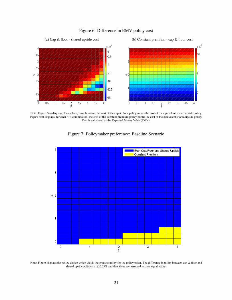
Figure 6: Difference in EMV policy cost

(a) Cap & floor - shared upside cost

0 0.5 1 1.5 2 2.5 3 3.5 40

0.5

1

1.5

2

2.5

3

3.5

4

β

α

−15

−10

−12.5

−7.5

−5

−2.5

−1

x 106

(b) Constant premium - cap & floor cost

0 0.5 1 1.5 2 2.5 3 3.5 40

1

2

3

4

β

α

2

4

6

8

10

x 108

Note: Figure 6(a) displays, for each α/β combination, the cost of the cap & floor policy minus the cost of the equivalent shared upside policy.

Figure 6(b) displays, for each α/β combination, the cost of the constant premium policy minus the cost of the equivalent shared upside policy.

Cost is calculated as the Expected Money Value (EMV).

Figure 7: Policymaker preference: Baseline Scenario

Note: Figure displays the policy choice which yields the greatest utility for the policymaker. The difference in utility between cap & floor and

shared upside policies is ≤ 0.03% and thus these are assumed to have equal utility.

21

that a constant premium results in a greater level of net utility for the policymaker when investor

risk is ≤ 0.5, whilst policymakers must have a risk aversion parameter of 0.75 or greater. As

expected levels of risk aversion hover about 1, this would suggest that investors must be indifferent

to risk for a constant premium policy to be optimal. This is an important finding in relation to

the common use of constant premium policies in many jurisdictions. This suggests that for such

policies to be optimal, policymakers must be more than four times as risk averse as investors. If

this is not the case, the disutility associated with the additional remuneration required for a constant

premium tariff is greater than the foregone disutility associated with an alternate FiT structure, and

thus a constant premium FiT is suboptimal.

This section has shown that intermediate division of market price risk is optimal when investor

and policymaker risk aversion is of a similar magnitude, with a difference of ≤ 0.07% between

utility for shared upside or cap & floor regimes. On utility grounds, both return similar values

under our baseline scenario. Modest cost differences occur when floor prices are low (likely to

occur when policymakers are highly risk averse and high levels of market upside are offered to

investors) and cap & floor policies thus result in a lower EMV cost. Constant premium policies

are considerably more expensive than both shared upside and cap & floor policies in EMV terms.

However, a constant premium policy may be preferred on utility grounds when investor’s risk

aversion is ≤ 0.5 and policymakers have risk aversion parameters in the region of 0.75 or greater.

A sensitivity analysis will now analyse results when alternate ranges of risk aversion or alternate

market conditions prevail.

5. Sensitivity analysis

Different levels of calibrated risk aversion may result in different degrees of optimal market

price risk apportionment. If FiT policy comprises a greater share of total electricity cost, poli-

cymakers may be more sensitive to bearing market price risk. Similarly, investor sensitivity may

increase if they have a less diversified portfolio of investments and thus require a higher EMV in

order to incentivise investment. Furthermore, the baseline scenario considered market price condi-

tions representative of deployment in Ireland, with results potentially sensitive to alternate market

assumptions. This section informs polcy as to optimal FiT choice under alternate scenarios of

calibrated risk aversion and market conditions.

We model a scenario of greater risk sensitivity by doubling the calibration parameters (wpolicypre

and winvpre) and model lesser sensitivity by halving the calibration parameters. ’Low sensitivity’

results are calculated where the calibration parameter is double the baseline level. For investor risk

aversion, this results in the baseline range of risk premia of figure 2 falling to a range of 2.34-39%,

with a value of 12% when α = 1. For policymaker risk aversion, the baseline range of risk premia

of table 2 fall to a range of 0.6-2.6%, with a value of 0.6% when β = 1. ’High sensitivity’ results

22

are calculated where the calibration parameter is half the baseline level. For investor risk aversion,

this results in the baseline range of risk premia of figure 2 rising to a range of 2.34-99%, with a

value of 34% when α = 1. For policymaker risk aversion, the baseline range of risk premia of table

2 rise to a range of 3-12.6%, with a value of 3% when β = 1.

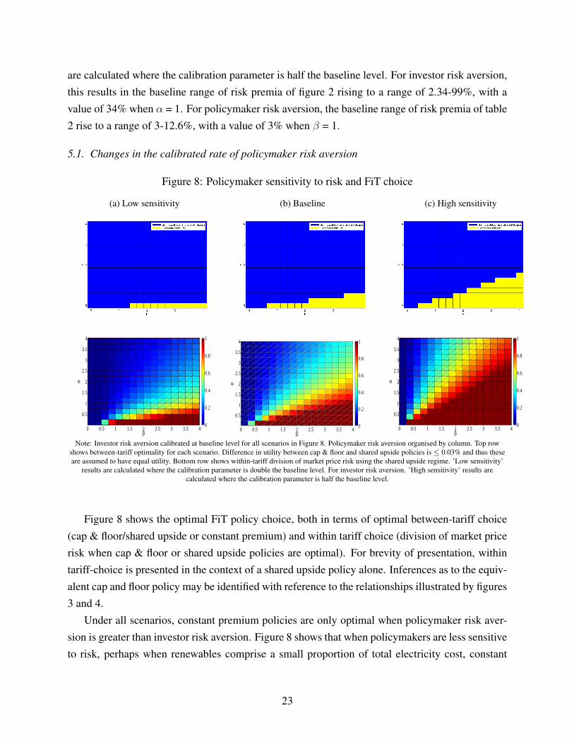
5.1. Changes in the calibrated rate of policymaker risk aversion

Figure 8: Policymaker sensitivity to risk and FiT choice

(a) Low sensitivity (b) Baseline (c) High sensitivity

0 0.5 1 1.5 2 2.5 3 3.5 4

0.5

1

1.5

2

2.5

3

3.5

4

β

α

0

0.2

0.4

0.6

0.8

1

0 0.5 1 1.5 2 2.5 3 3.5 4

0.5

1

1.5

2

2.5

3

3.5

4

α

β

0

0.2

0.4

0.6

0.8

1

0 0.5 1 1.5 2 2.5 3 3.5 4

0.5

1

1.5

2

2.5

3

3.5

4

β

α

0

0.2

0.4

0.6

0.8

1

Note: Investor risk aversion calibrated at baseline level for all scenarios in Figure 8. Policymaker risk aversion organised by column. Top row

shows between-tariff optimality for each scenario. Difference in utility between cap & floor and shared upside policies is ≤ 0.03% and thus these

are assumed to have equal utility. Bottom row shows within-tariff division of market price risk using the shared upside regime. ’Low sensitivity’

results are calculated where the calibration parameter is double the baseline level. For investor risk aversion. ’High sensitivity’ results are

calculated where the calibration parameter is half the baseline level.

Figure 8 shows the optimal FiT policy choice, both in terms of optimal between-tariff choice

(cap & floor/shared upside or constant premium) and within tariff choice (division of market price

risk when cap & floor or shared upside policies are optimal). For brevity of presentation, within

tariff-choice is presented in the context of a shared upside policy alone. Inferences as to the equiv-

alent cap and floor policy may be identified with reference to the relationships illustrated by figures

3 and 4.

Under all scenarios, constant premium policies are only optimal when policymaker risk aver-

sion is greater than investor risk aversion. Figure 8 shows that when policymakers are less sensitive

to risk, perhaps when renewables comprise a small proportion of total electricity cost, constant

23

premium policies are only optimal when investors are risk neutral. As policymakers are more sen-

sitive to FiT cost uncertainty, perhaps due to increased deployment or low fossil fuel costs and thus

a higher proportional burden, we find that constant premium policies are of greater importance.

When policymakers are highly sensitive, we find that constant premium policies are optimal when

investor risk aversion is around half that of policymaker risk aversion. As such, constant premium

policies are of increasing importance as the burden of renewables policy increases. However, even

with a doubling of the level of underlying sensitivity, constant premium policies are only optimal

when policymaker risk aversion is much greater than investor risk aversion.

Figure 8 also shows the division of market price risk when shared upside policies are chosen

for each of these policymaker wealth scenarios. When policymaker sensitivity is low, a flat rate

FiT or low share of market upside for investors is generally optimal. As policymakers become

more sensitive to market price risk, a higher θ/cap value and thus lower K guarantee is required

for efficient division of market price risk.

Figure 8 shows that as policymakers become more sensitive to market price risk, the optimal

division of market price risk evolves from zero to gradually incorporate varying degrees of market

upside for many risk aversion combinations. Such changes in sensitivity may occur due to an

increasing renewables subsidy burden as deployment progresses. For prudent forward-looking

policymakers, this finding shows that flexibility is required in legislative frameworks, such that

divisions of market price risk may be augmented to accommodate this evolving optimality.

5.1.1. Changes in the calibrated rate of investor risk aversion

Unlike changes in policymaker risk sensitivity, optimal constant premium policies will change

with changes in investor risk sensitivity. Figure 9 shows that a greater constant premium (X) is

required as investor risk sensitivity grows, with this difference greater for higher levels of risk

aversion.

Analysing between-policy FiT choice, Figure 10 shows that as investors become more sensitive

to market price risk, the scope for a constant premium FiT diminishes. This is in constrast to a

changes in policymaker risk sensitivity. As renewables deployment matures, FiT costs are likely

to comprise both a greater proportion of a policymaker’s electricity budget and a lesser proportion

of investors’ budgets, as larger, less specialised developers who are more diversified may enter the

industry. As such, investor risk aversion falls whilst policymaker risk aversion rises, suggesting

that the scope for premium policies may grow as both sensitivity analyses would suggest. Indeed,

if both investor sensitivity falls and policymaker sensitivity grows, the magnitude of this growth

may of an even greater extent than that described.

24

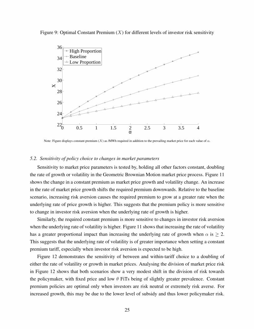
Figure 9: Optimal Constant Premium (X) for different levels of investor risk sensitivity

0 0.5 1 1.5 2 2.5 3 3.5 422

24

26

28

30

32

34

36X

α

High ProportionBaselineLow Proportion

Note: Figure displays constant premium (X) as /MWh required in addition to the prevailing market price for each value of α.

5.2. Sensitivity of policy choice to changes in market parameters

Sensitivity to market price parameters is tested by, holding all other factors constant, doubling

the rate of growth or volatility in the Geometric Brownian Motion market price process. Figure 11

shows the change in a constant premium as market price growth and volatility change. An increase

in the rate of market price growth shifts the required premium downwards. Relative to the baseline

scenario, increasing risk aversion causes the required premium to grow at a greater rate when the

underlying rate of price growth is higher. This suggests that the premium policy is more sensitive

to change in investor risk aversion when the underlying rate of growth is higher.

Similarly, the required constant premium is more sensitive to changes in investor risk aversion

when the underlying rate of volatility is higher. Figure 11 shows that increasing the rate of volatility

has a greater proportional impact than increasing the underlying rate of growth when α is ≥ 2.

This suggests that the underlying rate of volatility is of greater importance when setting a constant

premium tariff, especially when investor risk aversion is expected to be high.

Figure 12 demonstrates the sensitivity of between and within-tariff choice to a doubling of

either the rate of volatility or growth in market prices. Analysing the division of market price risk

in Figure 12 shows that both scenarios show a very modest shift in the division of risk towards

the policymaker, with fixed price and low θ FiTs being of slightly greater prevalence. Constant

premium policies are optimal only when investors are risk neutral or extremely risk averse. For

increased growth, this may be due to the lower level of subsidy and thus lower policymaker risk.

25

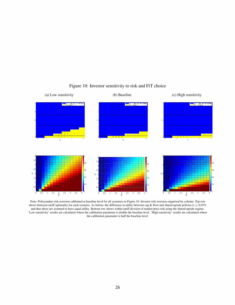
Figure 10: Investor sensitivity to risk and FiT choice

(a) Low sensitivity (b) Baseline (c) High sensitivity

0 0.5 1 1.5 2 2.5 3 3.5 4

0.5

1

1.5

2

2.5

3

3.5

4

β

α

0

0.2

0.4

0.6

0.8

1

0 0.5 1 1.5 2 2.5 3 3.5 4

0.5

1

1.5

2

2.5

3

3.5

4

α

β

0

0.2

0.4

0.6

0.8

1

0 0.5 1 1.5 2 2.5 3 3.5 40

1

2

3

4

β

α

0

0.2

0.4

0.6

0.8

1

Note: Policymaker risk aversion calibrated at baseline level for all scenarios in Figure 10. Investor risk aversion organised by column. Top row

shows between-tariff optimality for each scenario. As before, the difference in utility between cap & floor and shared upside policies is ≤ 0.03%

and thus these are assumed to have equal utility. Bottom row shows within-tariff division of market price risk using the shared upside regime.

’Low sensitivity’ results are calculated where the calibration parameter is double the baseline level. ’High sensitivity’ results are calculated where

the calibration parameter is half the baseline level.

26

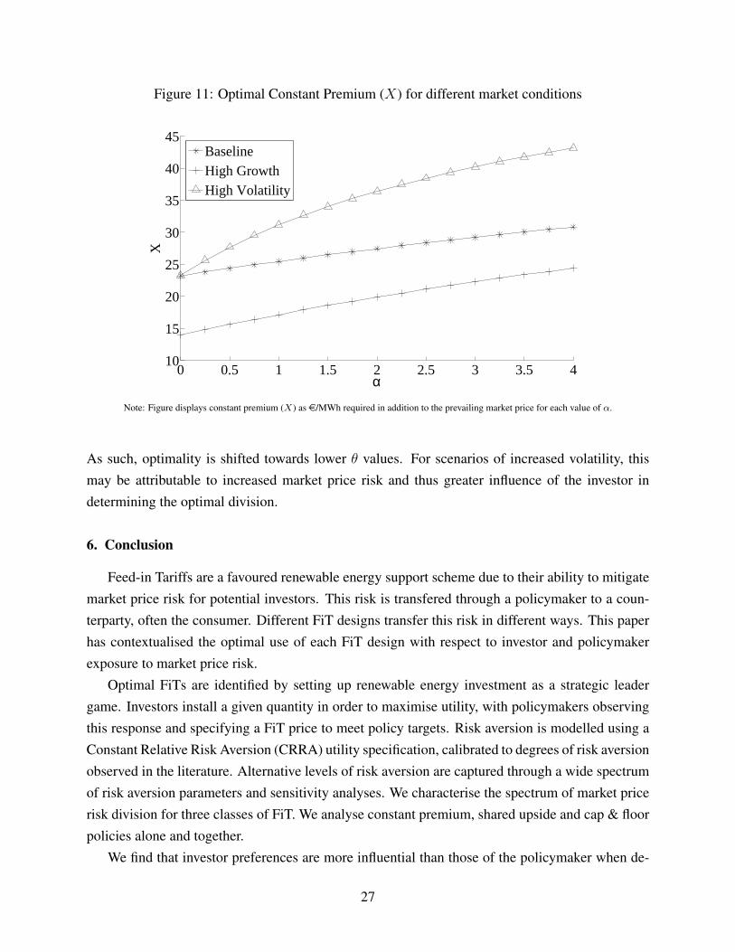
Figure 11: Optimal Constant Premium (X) for different market conditions

0 0.5 1 1.5 2 2.5 3 3.5 410

15

20

25

30

35

40

45X

α

BaselineHigh GrowthHigh Volatility

Note: Figure displays constant premium (X) as e/MWh required in addition to the prevailing market price for each value of α.

As such, optimality is shifted towards lower θ values. For scenarios of increased volatility, this

may be attributable to increased market price risk and thus greater influence of the investor in

determining the optimal division.

6. Conclusion

Feed-in Tariffs are a favoured renewable energy support scheme due to their ability to mitigate

market price risk for potential investors. This risk is transfered through a policymaker to a coun-

terparty, often the consumer. Different FiT designs transfer this risk in different ways. This paper

has contextualised the optimal use of each FiT design with respect to investor and policymaker

exposure to market price risk.

Optimal FiTs are identified by setting up renewable energy investment as a strategic leader

game. Investors install a given quantity in order to maximise utility, with policymakers observing

this response and specifying a FiT price to meet policy targets. Risk aversion is modelled using a

Constant Relative Risk Aversion (CRRA) utility specification, calibrated to degrees of risk aversion

observed in the literature. Alternative levels of risk aversion are captured through a wide spectrum

of risk aversion parameters and sensitivity analyses. We characterise the spectrum of market price

risk division for three classes of FiT. We analyse constant premium, shared upside and cap & floor

policies alone and together.

We find that investor preferences are more influential than those of the policymaker when de-

27

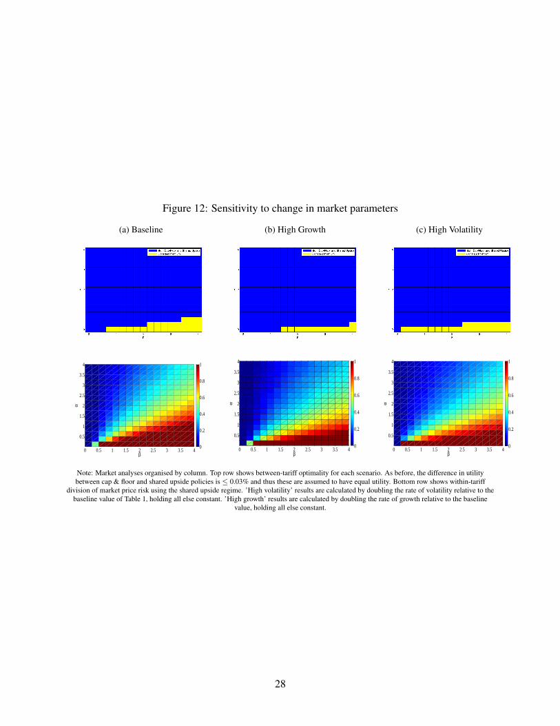
Figure 12: Sensitivity to change in market parameters

(a) Baseline (b) High Growth (c) High Volatility

0 0.5 1 1.5 2 2.5 3 3.5 4

0.5

1

1.5

2

2.5

3

3.5

4

α

β

0

0.2

0.4

0.6

0.8

1

0 0.5 1 1.5 2 2.5 3 3.5 4

0.5

1

1.5

2

2.5

3

3.5

4

β

α

0

0.2

0.4

0.6

0.8

1

0 0.5 1 1.5 2 2.5 3 3.5 4

0.5

1

1.5

2

2.5

3

3.5

4

β

α

0

0.2

0.4

0.6

0.8

1

Note: Market analyses organised by column. Top row shows between-tariff optimality for each scenario. As before, the difference in utility

between cap & floor and shared upside policies is ≤ 0.03% and thus these are assumed to have equal utility. Bottom row shows within-tariff

division of market price risk using the shared upside regime. ’High volatility’ results are calculated by doubling the rate of volatility relative to the

baseline value of Table 1, holding all else constant. ’High growth’ results are calculated by doubling the rate of growth relative to the baseline

value, holding all else constant.

28

grees of risk aversion are of a similar magnitude. Under our baseline assumptions, market price

risk should be shared except under circumstances of extreme investor/consumer indifference to

risk. This suggests that commonly employed fixed price and constant premium policies are sub-

optimal unless investors or consumers are risk neutral. We find that cap & floor policies offer a

similar but consistently lower level of utility to shared upside policies. This is because the dif-

ferent pattern of risk sharing requires a slightly lower minimum price guarantee under a cap &

floor regime. This impact is emphasised when efficient prices are lower, an occurrence which is

more likely to prevail when policymakers are extremely risk averse and investors are modestly

risk averse. In Expected Money Value (EMV) terms, constant premium policies are always more

expensive than those that share market upside, but offer higher utility when policymakers are risk

averse and investors have low levels of risk aversion. Efficient division of market price risk is of

increasing importance as policymakers and investors are more sensitive to market price risk, with

policymaker sensitivity of greater influence. Such sensitivity may change as renewables deploy-

ment grows and becomes a larger share of total electricity cost. For many risk aversion scenarios,

the optimal division of market price risk transitions through a wide spectrum of possible levels as

such sensitivity changes. This has implications for both current and future policymaking. First, this

suggests that consideration of optimal market price risk is of increasing importance as renewables

deployment grows. Second, current policy should anticipate such a potential requirement and put

in place flexible legislative measures to accommodate market price risk division if required.

Renewables deployment has continued at great pace in many jurisdictions, with FiTs the pre-

dominant support measure and growing in influence. Cited as a hedge against fossil fuel market

price fluctuations, the relative benefit of renewables has been under increasing strain with the inter-

national proliferation of low-cost unconventional gas and depressing effect this has had on electric-

ity prices. Not only has this potentially reduced the hedge value of renewables, the potential risk

of high subsidy cost has become a greater concern in many jurisdictions. Such concerns may grow

with increasing renewables penetration. This paper presents a means for policymakers to consider

environmental policy in the context of such risks. Through the modelling framework presented, we

provide an economic rationale for optimal FiT specification with which a policymaker may make

a more informed decision as to both the level and format of a chosen FiT.

Acknowledgements

This work was funded under the Programme for Research in Third-Level Institutions (PRTLI)

Cycle 5 and co-funded under the European Regional Development Fund (ERDF); Science Founda-

tion Ireland awards 09/SRC/E1780 and 12/IA/1683. The authors would like to thank Sean Lyons

and James Gleeson for helpful comments, along with participants at the 2014 Mannheim Energy

29

Conference and the 2014 Annual Conference of the Irish Economic Association. The usual dis-

claimer applies.

References

Anderson, J. R., Dillon, J. L., 1992. Risk analysis in dryland farming systems. No. 2. Food &

Agriculture Org.

Arrow, K., 1971. Essays in the theory of risk-bearing. North-Holland.

Arrow, K. J., 1965. Aspects of the Theory of Risk-Bearing. Yrjo Jahnssonin Saatio , Academic

Bookstore, Helsinki.

Batlle, C., 2011. A method for allocating renewable energy source subsidies among final energy

consumers. Energy Policy 39 (5), 2586 – 2595.

URL http://www.sciencedirect.com/science/article/pii/S0301421511001078

Bryant, C., 2013. Soaring renewable energy costs set to stoke german energy debate. Financial

Times.

Burer, M. J., Wustenhagen, R., 2009. Which renewable energy policy is a venture capitalist’s best

friend? empirical evidence from a survey of international cleantech investors. Energy Policy

37 (12), 4997 – 5006.

URL http : //www.sciencedirect.com/science/article/pii/S0301421509004807

Butler, L., Neuhoff, K., 2008. Comparison of feed-in tariff, quota and auction mechanisms to

support wind power development. Renewable Energy 33 (8), 1854 – 1867.


Chang, M.-C., Hu, J.-L., Han, T.-F., 2013. An analysis of a feed-in tariff in taiwans electricity

market. International Journal of Electrical Power & Energy Systems 44 (1), 916–920.

URL http : //linkinghub.elsevier.com/retrieve/pii/S0142061512004863

Chawla, M., Pollitt, M. G., Jan. 2013. Energy-efficiency and environmental policies & income

supplements in the UK: evolution and distributional impacts on domestic energy bills 2 (1).

URL http : //www.iaee.org/en/publications/eeeparticle.aspx?id = 39

Chronopoulos, M., Reyck, B. D., Siddiqui, A., 2014. Duopolistic competition under risk aversion

and uncertainty. European Journal of Operational Research 236 (2), 643 – 656.


30

Cotter, J., Hanly, J., 2012. A utility based approach to energy hedging. Energy Economics 34 (3),

817–827.

URL http : //ideas.repec.org/a/eee/eneeco/v34y2012i3p817− 827.html

Couture, T., Gagnon, Y., 2010. An analysis of feed-in tariff remuneration models: Implications for

renewable energy investment. Energy Policy 38 (2), 955–965.


Devitt, C., Malaguzzi Valeri, L., 2011. The effect of refit on irish wholesale electricity prices. The

Economic and Social Review 42 (3), 343369.

URL http : //ideas.repec.org/a/eso/journl/v42y2011i3p343− 369.html

Dinica, V., 2006. Support systems for the diffusion of renewable energy technologiesan investor

perspective. Energy Policy 34 (4), 461 – 480.


Doherty, R., O’Malley, M., 2011. The efficiency of Ireland’s Renewable Energy Feed-In Tariff

(REFIT) for wind generation. Energy Policy 39 (9), 4911–4919.


Dong, C., 2012. Feed-in tariff vs. renewable portfolio standard: An empirical test of their relative

effectiveness in promoting wind capacity development. Energy Policy 42 (0), 476 – 485.


DW, 2013. German energy transition caught in subsidies’ trap. DW.de.

Ekins, P., 2004. Step changes for decarbonising the energy system: research needs for renewables,

energy efficiency and nuclear power. Energy Policy 32 (17), 1891–1904.


Energy Information Administration, 2012. Annual energy outlook 2012. Tech. rep., U.S. Depart-

ment of Energy, Washington, DC .

URL http : //www.eia.gov/forecasts/aeo/pdf/0383(2012).pdf

Fagiani, R., Barqun, J., Hakvoort, R., 2013. Risk-based assessment of the cost-efficiency and

the effectivity of renewable energy support schemes: Certificate markets versus feed-in tariffs.

Energy Policy 55 (0), 648 – 661, special section: Long Run Transitions to Sustainable Economic

Structures in the European Union and Beyond.


31

Falconett, I., Nagasaka, K., 2010. Comparative analysis of support mechanisms for renewable

energy technologies using probability distributions. Renewable Energy 35 (6), 1135 – 1144.


Farrell, N., Devine, M., Lee, W., Gleeson, J., Lyons, S., Sep. 2013. Specifying an efficient renew-

able energy feed-in tariff. MPRA Paper 49777, University Library of Munich, Germany.

URL http : //ideas.repec.org/p/pra/mprapa/49777.html

Farrell, N., Lyons, S., 2014. The distributional impact of the irish public service obligation levy on

electricity consumption. MPRA Paper 53488, University Library of Munich, Germany.

URL http : //ideas.repec.org/p/pra/mprapa/53488.html

Fudenberg, D., Tirole, J., 1991. Game theory. MIT Press, Cambridge, Massachusetts.

Gross, R., Blyth, W., Heptonstall, P., 2010. Risks, revenues and investment in electricity gener-

ation: Why policy needs to look beyond costs. Energy Economics 32 (4), 796 – 804, policy-

making Benefits and Limitations from Using Financial Methods and Modelling in Electricity

Markets.


Haas, R., Resch, G., Panzer, C., Busch, S., Ragwitz, M., Held, A., 2011. Efficiency and effec-

tiveness of promotion systems for electricity generation from renewable energy sources lessons

from {EU} countries. Energy 36 (4), 2186 – 2193, 5th Dubrovnik Conference on Sustainable

Development of Energy, Water & Environment Systems.


Hardaker, J., Huirne, R., Anderson, J., Lien, G., et al., 2004. Coping with risk in agriculture, second

edition. CABI Publishing.

Hern, R., Radov, D., Bermudez-Neubauer, M., Brejnholt, R., Huebler, D., Spasovska, M.,

Janeckova, Z., Tannenbaum, B., Fearnehough, H., 2013. Changes in hurdle rates for low carbon

generation technologies due to the shift from the uk renewables obligation to a contracts for

difference regime. Tech. rep., London: NERA Economic Consulting.

URL http : //www.nera.com/nera−files/20131209NERAReportAssessmentofChangeinHurdleRates.pd

Heydari, S., Ovenden, N., Siddiqui, A., 2012. Real options analysis of investment in carbon capture

and sequestration technology. Computational Management Science 9 (1), 109–138.

URL http : //dx.doi.org/10.1007/s10287− 010− 0124− 5

Hirst, E., 2002. The financial and physical insurance benefits of price-responsive demand. The

Electricity Journal 15 (4), 66–73.

32

IEA and OECD, 2008. Deploying renewables principles for effective policies: in support of the G8

plan of action. IEA and OECD, Paris.

URL http : //www.myilibrary.com?id = 192197

IWEA, 2011. The impact of wind on pricing within the Single Electricity Market.

URL http : //www.iwea.com/contentF iles/Documents%20for%20Download/Publications/News%20I

1298912434703

Kim, K.-K., Lee, C.-G., 2012. Evaluation and optimization of feed-in tariffs. Energy Policy 49,

192–203.


Kitzing, L., 2014. Risk implications of renewable support instruments: Comparative analysis of

feed-in tariffs and premiums using a meanvariance approach. Energy 64 (0), 495 – 505.


Kitzing, L., Mitchell, C., Morthorst, P. E., Dec. 2012. Renewable energy policies in europe: Con-

verging or diverging? Energy Policy 51, 192–201.

URL http : //linkinghub.elsevier.com/retrieve/pii/S030142151200746X

Klessmann, C., Rathmann, M., de Jager, D., Gazzo, A., Resch, G., Busch, S., Ragwitz, M., 2013.

Policy options for reducing the costs of reaching the european renewables target. Renewable

Energy 57 (0), 390 – 403.


Leepa, C., Unfried, M., 2013. Effects of a cut-off in feed-in tariffs on photovoltaic capacity:

Evidence fromgermany. Energy Policy 56 (0), 536 – 542.


Logan, J., Lopez, A., Mai, T., Davidson, C., Bazilian, M., Arent, D., 2013. Natural gas scenarios

in the us power sector. Energy Economics 40, 183–195.

Loreck, C., Matthes, F., Hermann, H., Jung, F., Emele, L., Cook, V., 2012. Short analysis of the

increase of the german eeg surcharge for 2013. Tech. rep., Berlin: ko-Institut e.V.

URL http : //www.oeko.de/oekodoc/1607/2012− 461− en.pdf

Ma, C.-T. A., McGuire, T. G., 1997. Optimal health insurance and provider payment. The Ameri-

can Economic Review 87 (4), pp. 685–704.

URL http://www.jstor.org/stable/2951369

33

Mahul, O., 2001. Optimal insurance against climatic experience. American Journal of Agricultural

Economics 83 (3), pp. 593–604.


Mc Garrigle, E., Deane, J., Leahy, P., 2013. How much wind energy will be curtailed on the 2020

irish power system? Renewable Energy 55, 544–553.


Menanteau, P., Finon, D., Lamy, M.-L., Jun. 2003. Prices versus quantities: choosing policies for

promoting the development of renewable energy. Energy Policy 31 (8), 799–812.


Meyer, D., Meyer, J., 2005. Relative risk aversion: What do we know? Journal of Risk and

Uncertainty 31 (3), 243–262.

URL http://dx.doi.org/10.1007/s11166-005-5102-x

Ragwitz, M., Held, A., Resch, G., Faber, T., Haas, R., Huber, C., Coenraads, R., Voogt, M., Reece,

G., Morthorst, P., Jensen, S., Konstantinaviciute, I., Heyder, B., 2007. Assessment and Optimiza-

tion of Renewable Energy Support Schemes in the European Electricity Market: Final Report.

Optimization of Renewable Energy Support (OPTRES) project for the European Commission,

DG TREN, and Intelligent Energy for Europe (IEE), Karlsruhe, Germany.

Rauch, J. N., 2013. The effect of different market conditions on the hedge value of long-term

contracts for zero-fuel-cost renewable resources. The Electricity Journal 26 (5), 44 – 51.


Raviv, A., 1979. The design of an optimal insurance policy. The American Economic Review

69 (1), pp. 84–96.


Ringel, M., 2006. Fostering the use of renewable energies in the european union: the race between

feed-in tariffs and green certificates. Renewable Energy 31 (1), 1 – 17.


SEAI, 2011. Seai wind energy roadmap 2011-2050. Report of the SEAI Energy Modelling Group.

Sensfuß, F., Ragwitz, M., Genoese, M., 2008. The merit-order effect: A detailed analysis of the

price effect of renewable electricity generation on spot market prices in germany. Energy Policy

36 (8), 3086–3094.


34

von Neumann, J., Morgenstern, O., 1947. The Theory of Games and Economic Behavior. Princeton

University Press.

Yang, M., Blyth, W., 2007. Modeling investment risks and uncertainties with real options approach.

International Energy Agency.

Zhang, Q., Wang, X., Aug 2009. Hedge contract characterization and risk-constrained electricity

procurement. Power Systems, IEEE Transactions on 24 (3), 1547–1558.

Zhu, L., 2012. A simulation based real options approach for the investment evaluation of nuclear

power. Computers & Industrial Engineering 63 (3), 585–593.

35