Managing Inventory of Items with Replacement

Warranty

Wei Huang † Vidhyadhar Kulkarni †1

Jayashankar M. Swaminathan †‡1

Department of Statistics and Operations Research †

The Kenan-Flagler Business School ‡

University of North Carolina, Chapel Hill, NC 27599

June 2005; Revised August 2005

Abstract

In this paper we study a firm that faces demand from two sources: demand

for new products and demand to replace failed items under warranty. We model

this setting as a multi-period single product inventory problem where the new

demand in different periods are independent and the demand for replacing failed

items is dependent on the number and age of items under warranty. We consider

backlogging and emergency supply cases, and study both discounted cost and av-

erage cost cases. We prove the optimality of the w-dependent base stock ordering

policy where the base stock level is a function of w, the vector representing the

number of items at different ages currently under warranty. For the special case,

where the demand for new products is stationary, we prove the optimality of a

stationary w-dependent base stock policy for the finite horizon discounted and the

infinite horizon discounted and average cost cases. In our computational study,

we find that an optimal integrated policy can lead to 37% average improvement in

expected costs when compared to a policy that neglects warranty repairs.

Keyword: Warranty, Inventory, Stochastic Demand, Information.

1This work is partially supported by NSF Grant DMII-0223117.

1

1 Introduction

As firms attempt to optimize their end to end supply chains, their focus is turning to-

wards the close-loop nature of supply chain operations (see Guide and Wassenhove ([11]),

Dekker, Fleischmann, Inderfurth, and Wassenhove ([6])). Firms are actively integrating

their after-sale parts and services with their forward supply chain processes. One such

initiative has been to incorporate field installation and failure information into supply

chain planning and operations. Sciorrotta ([19]) emphasizes the importance of SiRAS

(www.siras.com), a patented electronic registration program which captures a product’s

serial number at point of sale. This system used by Wal-Mart and Target enables man-

ufacturers to keep track of warranty age information for the items thereby helping them

prepare inventory and production capacity for repairs. In addition, as the RFID technol-

ogy develops, it is projected that RFID chips could be utilized extensively for tracking

machine status in the field and performing proactive maintenance thereby leading to

significant improvements in supply chain performance (see EPCglobal ([8])).

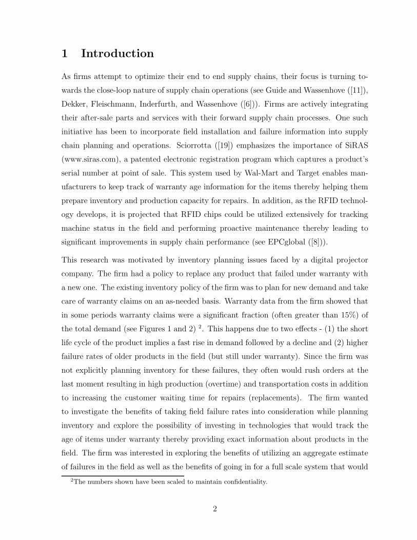
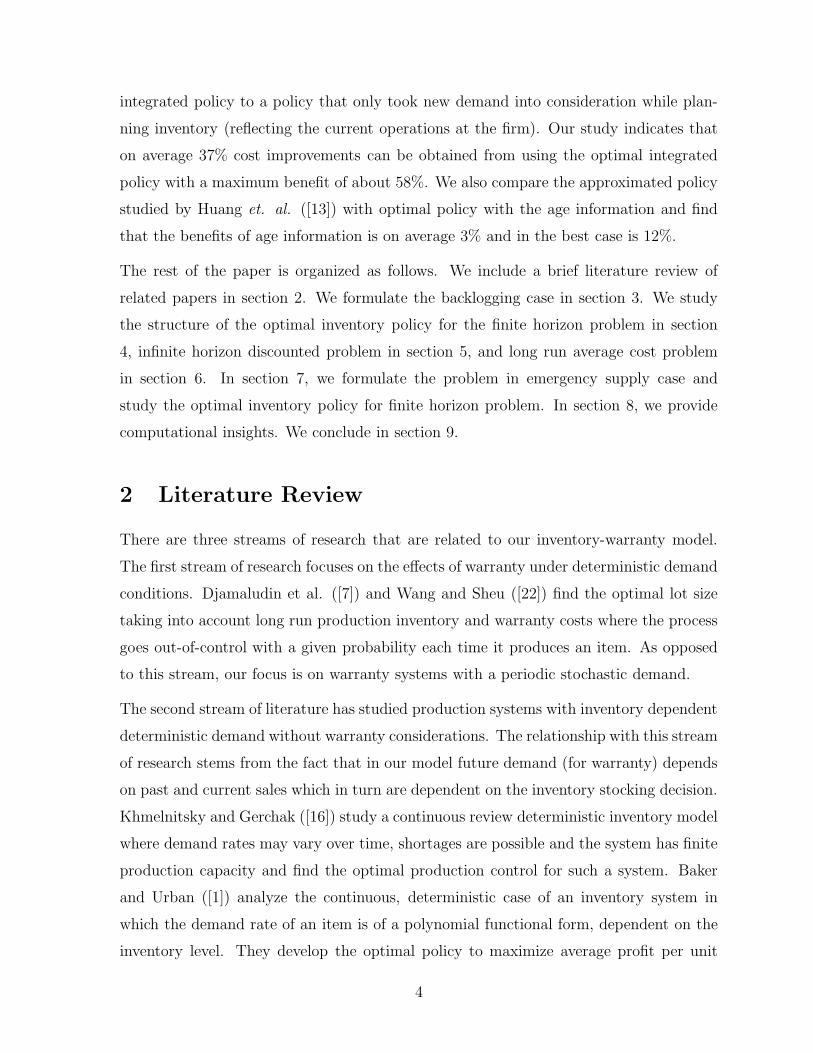
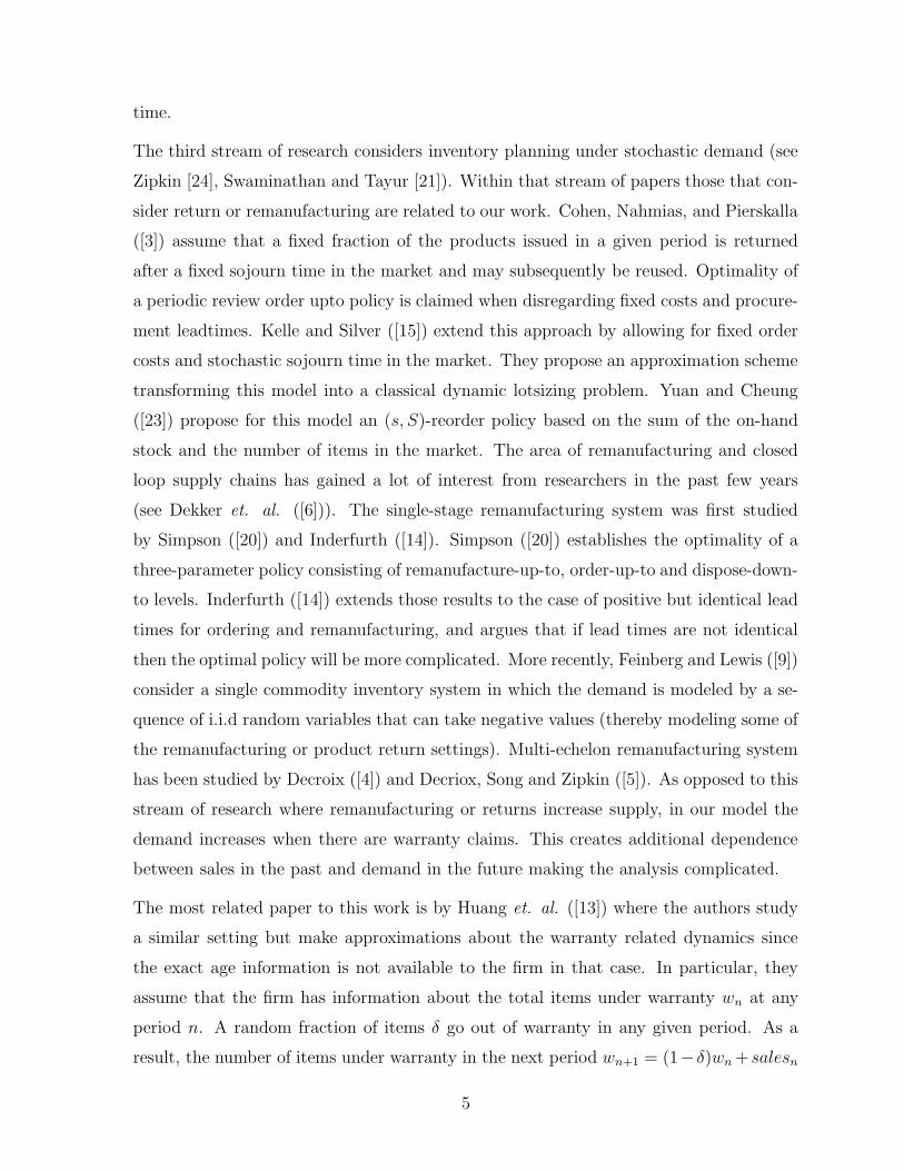
This research was motivated by inventory planning issues faced by a digital projector

company. The firm had a policy to replace any product that failed under warranty with

a new one. The existing inventory policy of the firm was to plan for new demand and take

care of warranty claims on an as-needed basis. Warranty data from the firm showed that

in some periods warranty claims were a significant fraction (often greater than 15%) of

the total demand (see Figures 1 and 2) 2. This happens due to two effects - (1) the short

life cycle of the product implies a fast rise in demand followed by a decline and (2) higher

failure rates of older products in the field (but still under warranty). Since the firm was

not explicitly planning inventory for these failures, they often would rush orders at the

last moment resulting in high production (overtime) and transportation costs in addition

to increasing the customer waiting time for repairs (replacements). The firm wanted

to investigate the benefits of taking field failure rates into consideration while planning

inventory and explore the possibility of investing in technologies that would track the

age of items under warranty thereby providing exact information about products in the

field. The firm was interested in exploring the benefits of utilizing an aggregate estimate

of failures in the field as well as the benefits of going in for a full scale system that would

2The numbers shown have been scaled to maintain confidentiality.

2

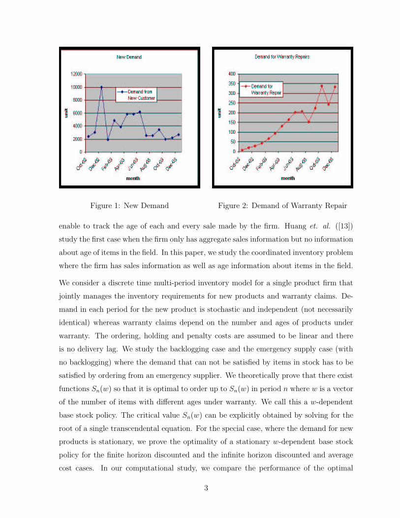
Figure 1: New Demand Figure 2: Demand of Warranty Repair

enable to track the age of each and every sale made by the firm. Huang et. al. ([13])

study the first case when the firm only has aggregate sales information but no information

about age of items in the field. In this paper, we study the coordinated inventory problem

where the firm has sales information as well as age information about items in the field.

We consider a discrete time multi-period inventory model for a single product firm that

jointly manages the inventory requirements for new products and warranty claims. De-

mand in each period for the new product is stochastic and independent (not necessarily

identical) whereas warranty claims depend on the number and ages of products under

warranty. The ordering, holding and penalty costs are assumed to be linear and there

is no delivery lag. We study the backlogging case and the emergency supply case (with

no backlogging) where the demand that can not be satisfied by items in stock has to be

satisfied by ordering from an emergency supplier. We theoretically prove that there exist

functions Sn(w) so that it is optimal to order up to Sn(w) in period n where w is a vector

of the number of items with different ages under warranty. We call this a w-dependent

base stock policy. The critical value Sn(w) can be explicitly obtained by solving for the

root of a single transcendental equation. For the special case, where the demand for new

products is stationary, we prove the optimality of a stationary w-dependent base stock

policy for the finite horizon discounted and the infinite horizon discounted and average

cost cases. In our computational study, we compare the performance of the optimal

3

integrated policy to a policy that only took new demand into consideration while plan-

ning inventory (reflecting the current operations at the firm). Our study indicates that

on average 37% cost improvements can be obtained from using the optimal integrated

policy with a maximum benefit of about 58%. We also compare the approximated policy

studied by Huang et. al. ([13]) with optimal policy with the age information and find

that the benefits of age information is on average 3% and in the best case is 12%.

The rest of the paper is organized as follows. We include a brief literature review of

related papers in section 2. We formulate the backlogging case in section 3. We study

the structure of the optimal inventory policy for the finite horizon problem in section

4, infinite horizon discounted problem in section 5, and long run average cost problem

in section 6. In section 7, we formulate the problem in emergency supply case and

study the optimal inventory policy for finite horizon problem. In section 8, we provide

computational insights. We conclude in section 9.

2 Literature Review

There are three streams of research that are related to our inventory-warranty model.

The first stream of research focuses on the effects of warranty under deterministic demand

conditions. Djamaludin et al. ([7]) and Wang and Sheu ([22]) find the optimal lot size

taking into account long run production inventory and warranty costs where the process

goes out-of-control with a given probability each time it produces an item. As opposed

to this stream, our focus is on warranty systems with a periodic stochastic demand.

The second stream of literature has studied production systems with inventory dependent

deterministic demand without warranty considerations. The relationship with this stream

of research stems from the fact that in our model future demand (for warranty) depends

on past and current sales which in turn are dependent on the inventory stocking decision.

Khmelnitsky and Gerchak ([16]) study a continuous review deterministic inventory model

where demand rates may vary over time, shortages are possible and the system has finite

production capacity and find the optimal production control for such a system. Baker

and Urban ([1]) analyze the continuous, deterministic case of an inventory system in

which the demand rate of an item is of a polynomial functional form, dependent on the

inventory level. They develop the optimal policy to maximize average profit per unit

4

time.

The third stream of research considers inventory planning under stochastic demand (see

Zipkin [24], Swaminathan and Tayur [21]). Within that stream of papers those that con-

sider return or remanufacturing are related to our work. Cohen, Nahmias, and Pierskalla

([3]) assume that a fixed fraction of the products issued in a given period is returned

after a fixed sojourn time in the market and may subsequently be reused. Optimality of

a periodic review order upto policy is claimed when disregarding fixed costs and procure-

ment leadtimes. Kelle and Silver ([15]) extend this approach by allowing for fixed order

costs and stochastic sojourn time in the market. They propose an approximation scheme

transforming this model into a classical dynamic lotsizing problem. Yuan and Cheung

([23]) propose for this model an (s, S)-reorder policy based on the sum of the on-hand

stock and the number of items in the market. The area of remanufacturing and closed

loop supply chains has gained a lot of interest from researchers in the past few years

(see Dekker et. al. ([6])). The single-stage remanufacturing system was first studied

by Simpson ([20]) and Inderfurth ([14]). Simpson ([20]) establishes the optimality of a

three-parameter policy consisting of remanufacture-up-to, order-up-to and dispose-down-

to levels. Inderfurth ([14]) extends those results to the case of positive but identical lead

times for ordering and remanufacturing, and argues that if lead times are not identical

then the optimal policy will be more complicated. More recently, Feinberg and Lewis ([9])

consider a single commodity inventory system in which the demand is modeled by a se-

quence of i.i.d random variables that can take negative values (thereby modeling some of

the remanufacturing or product return settings). Multi-echelon remanufacturing system

has been studied by Decroix ([4]) and Decriox, Song and Zipkin ([5]). As opposed to this

stream of research where remanufacturing or returns increase supply, in our model the

demand increases when there are warranty claims. This creates additional dependence

between sales in the past and demand in the future making the analysis complicated.

The most related paper to this work is by Huang et. al. ([13]) where the authors study

a similar setting but make approximations about the warranty related dynamics since

the exact age information is not available to the firm in that case. In particular, they

assume that the firm has information about the total items under warranty wn at any

period n. A random fraction of items δ go out of warranty in any given period. As a

result, the number of items under warranty in the next period wn+1 = (1− δ)wn + salesn

5

where salesn is total sales of new and warrantied items in period n. Once we assume

that ages of different items under warranty are known (as in our model), the actual items

going out of warranty is known exactly every period as well as the failure rate of items

can be approximated more accurately by incorporating age dependent failure rates. This

increases the state space vector and complicates the analysis. Nevertheless, we are able

to characterize the optimal inventory policy.

3 Model with Backlogging

In our model inventory for a single product is managed for multiple periods. The firm

offers replacement of items that fail under warranty. The demand arises from two sources:

new demand, and demand to replace failed items under warranty. In this paper, we focus

on a fixed-period warranty policy, i.e., any item above age K is out of warranty. Let

wn,j be the number of items at age j under warranty at period n for j = 1, · · · , K.

wn as a vector [wn,1, · · · , wn,K]. Let ζn be the new demand in period n and Fn(.) be

its cumulative distribution function (cdf), and fn(.) be its probability density function

(pdf). Let xn be the inventory on hand at the beginning of period n, and yn be the

inventory immediately after an order is delivered at period n. We treat yn ≥ xn as the

decision variable in period n. The delivery is assumed to be instantaneous, so that yn

is the amount available to satisfy the demand for new and warranty claims in period n.

Any demand that can not be immediately satisfied is backlogged.

We assume that warranty is renewable, i.e., the warranty period of the replaced item

starts afresh. Such warranty models have been studied in the past (see Blischke and

Murthy ([2])). We also assume that the demand to replace failed items is based on a

proportional model i.e. a fixed fraction βj of the items at age j under warranty fail

for j = 1, · · · , K, and let β = [β1, β2, · · · , βK] be the vector of these failure fractions.

This is a common assumption in warranty models and follows from bernoulli failures.

Different βj allow us to capture age dependent failure rates for different items in the

field. Although getting accurate estimates for the βj is not easy, with investment in

RFID chips it is possible to track the failures associated with a product. As a result

these estimates would be more readily available in future. Further, all the items that are

K periods old go out of warranty in the next period.

6

We assume that there is a per unit procurement cost c, holding cost h for each item

remaining at the end of a period, and shortage cost p for each unit of backlogged demand

in any period. We assume that at the end of planning horizon, the unit salvage cost is c

as well. Let

Ln(w, y) =

p∫ ∞

ζ=y−β·w(ζ − y + β · w)fn(ζ)dζ

+h∫ y−β·w

ζ=0(y − ζ − β · w)fn(ζ)dζ if y ≥ β · w

p∫ ∞

ζ=0(ζ − y + β · w)fn(ζ)dζ, o.w.

(1)

represent the expected penalty and holding cost incurred in period n if wn = w, yn = y

(Here β · w =∑

j βjwj denotes the scalar product of β and w.) The total one period

expected cost incurred for ordering up to y is given by

Cn(w, x, y) = c(y − x) + Ln(w, y),

where y ≥ x.

The dynamics of the situation implies that

wn+1,1 = min(yn, β · wn + ζn)

wn+1,j = wn,j−1(1 − βj−1) for j = 2, · · · , K (2)

xn+1 = yn − ζn − β · wn.

Thus {((wn, xn), yn), n ≥ 0} is a Markov decision process.

Let α, 0 ≤ α ≤ 1 be the discount factor and π be any policy for choosing decision yn

at time n, based on the history up to time n. We consider three objective functions for

choosing an optimal policy as described below.

1. Finite Horizon. The first objective of the firm is to minimize the expected total

discounted cost (ETDC) over periods 0, 1, 2, · · · , N . Let V πN (w, x) be the ETDC of fol-

lowing the policy π over periods 0, 1, · · · , N . Since we have a finite horizon we need to

specify the terminal cost. Let T (wN , xN) be the terminal cost at time N . Thus

V πN (w, x) = Eπ(

N−1∑

n=0

αnCn(wn, xn, yn) + αNT (wN , xN )|w0 = w, x0 = x)

Here Eπ denotes the expectation under the assumption that the policy π is followed. Let

VN(w, x) be the optimal ETDC of operating the system over period 0, · · · , N . That is

VN(w, x) = infπ

V πN (w, x). (3)

7

A policy π∗ is called optimal for finite horizon ETDC if

VN(w, x) = V π∗

N (w, x) for all w and x.

2. Infinite Horizon ETDC. The second objective function is to minimize the ETDC

over the infinite horizon. In this case there is no terminal cost function. Let V π(w, x) be

the infinite horizon ETDC of following policy π, that is

V π(w, x) = Eπ(

∞∑

n=0

αnCn(wn, xn, yn)|w0 = w, x0 = x)

Similarly, let V (w, x) be the optimal infinite horizon ETDC, that is

V (w, x) = infπ

V π(w, x).

A policy π∗ is called optimal for infinite horizon ETDC if

V (w, x) = V π∗

(w, x) for all w and x.

3. Infinite Horizon Average Cost. Let gπ(w, x) be the expected cost per period of

following policy π over infinite horizon starting from state (w, x). Again, there is no

terminal cost in this formulation. Thus assuming the limit exists,

gπ(w, x) = limN→∞

1

N + 1Eπ(

N∑

n=0

Cn(wn, xn, yn)|w0 = w, x0 = x).

Let g(w, x) be the optimal expected cost per period over infinite horizon starting in state

(w, x). That is,

g(w, x) = infπ

gπ(w, x).

A policy π∗ is called optimal for infinite horizon average cost if

V (w, x) = V π∗

(w, x) for all w and x.

4 Finite Horizon Discounted Cost

In this section, we study the finite horizon problem with N periods, terminal cost T (w, x),

and show how to compute VN(w, x) of Equation (3). First define Vn,N(w, x) to be the

8

optimal ETDC over periods n, n + 1, · · · , N starting with w = [w1, · · · , wK] units under

warranty and x units inventory at the beginning of period n. Let Gn,N(w, y) be the

ETDC over periods over n, n + 1, · · · , N given w units under warranty, and order upto

level y units at the beginning to period n. Then the standard dynamic programming

recursion yields

VN,N(w, x) = T (w, x)

Gn,N(w, y)

= cy + αLn(w, y)

+ α

∫ y−β·w

0

Vn+1,N(β · w + ζ, w1(1 − β1), · · · , wK−1(1 − βK−1), y − β · w − ζ)fn(ζ)dζ

+ α

∫ ∞

y−β·w

Vn+1,N(y, w1(1 − β1), · · · , wK−1(1 − βK−1), y − β · w − ζ)fn(ζ)dζ

Vn,N(w, x) = miny≥x

{Gn,N(w, y)} − cx, n = 0, 1, · · · , N − 1. (4)

where Ln(w, y) is as in Equation (1). Then we have

VN (w, x) = V0,N(w, x)

In any finite horizon inventory problem, we need to specify a terminal cost. In our case,

the terminal cost depends on wj (j = 1 · · ·K) as well as the remaining inventory x at

the end of the horizon. Although the product has a short life cycle in terms of sales,

the warranty claims may extend over a much longer period. For example, in the case

of personal computers the product life cycle for sales is close to a year but due to high

quality and reliability of machines a typical personal computer may last for several years.

When the warranty is renewable as in our case, this may extend for an infinite period.

Consider an item of age j at time N . Let mj be the total expected discounted cost of

warranty claims for this item incurred from N onwards. The following proposition Gives

the expressions for mi, 1 ≤ i ≤ K. The proof is given in the appendix.

Proposition 1 Let

θi =

K∑

j=i

αj−icβjΠj−1d=i(1 − βd) for i = 1, · · · , K.

Then mi, 1 ≤ i ≤ K are given by

m1 =cθ1

1 − αθ1

mi = θic + αθim1 for i = 2, · · · , K.

9

We propose the following terminal cost function T (w, x) when there are wi items of age

i, and x items in the inventory left on hand at the end of horizon:

T (w, x) =K

∑

j=i

mjwj − cx. (5)

The first term represents the expected discounted cost of warranty claims of the wi items

under warranty in period N at age i = 1, · · · , K, incurred over the infinite time from

then on. The term −cx reflects the assumption that any leftover inventory at period can

be returned at original price c and any shortages at the end of the horizon can be fulfilled

by purchasing products at c per unit. The detailed proof is in the Appendix. Here is

some additional notation for our analysis.

w1 = min(y, β · w + ζ),

wj = wj−1(1 − βj−1) for j = 2, · · · , K,

w = [w1, · · · , wK],

x = y − β · w − ζ,

p = p − m1,

Sn(w) = β · w + F−1n (

p − c(1 − α)

p + h), (6)

Ln(w, y) = h

∫ y−β·w

0

(y − β · w − ζ)fn(ζ)dζ + p

∫ ∞

y−β·w

(ζ − y + β · w)fn(ζ)dζ,

τn(w, y) = y − β · w − Sn(w),

∆n = α(m1 + c)µn + c(1 − α)F−1n (

p − c(1 − α)

p + h)

+ αLn(w, Sn(w)). (7)

Let µn be the mean demand from new customers at period n. Now let,

HN(w, x) = 0,

Hn(w, x) =

0 if x ≤ Sn(w)

Gn,N(w, x) − Gn,N(w, Sn(w)), o.w.

for 0 ≤ n ≤ N − 1 (8)

The next theorem establishes the optimality of the w-dependent base-stock policy in the

finite horizon case.

10

Theorem 1 Suppose the demands in each period are stochastically increasing, i.e.,

Fn(x) ≥ Fn+1(x), for n = 0, · · · , N − 2. (9)

Then

(i) Gn,N(w, y) = c(1 − α)y + αLn(w, y) + (α∆n+1 + · · · + αn−1∆N )

+ α(m · w) + α(m1 + c)µn

+ α

∫ τn+1(w,y)

0

Hn+1(w, x)fn(ζ)dζ, (10)

for n = 0, · · · , N − 1. y = Sn(w) minimizes Gn,N(w, y) for n = 0, · · · , N − 1, and

Gn,N(w, y) increases with respect to y when y ≥ Sn(w).

(ii)∫ τn(w,y)

0Hn(w, x)fn−1(ζ)dζ is an increasing function of y when y ≥ Sn−1(w) for a

given w for n = 0, · · · , N − 1.

(iii) Vn,N(w, x) = m · w − cx + (∆n + α∆n+1 + · · ·+ αn−1∆N) + Hn(w, x) (11)

for n = 0, · · · , N − 1.

Establishing the above theorem in the case with warranties is more involved than the

standard inventory problem because Gn,N(w, y) may not be convex in y. The particular

terminal cost function of Equation (5) enables us to establish the result by writing the

function as a sum of two other functions: the first one is convex in y and is minimized

at Sn(w) (defined by Equation (6)) and the second one is constant for y ≤ Sn(w) and

increases with y for y ≥ Sn(w) and thus achieves its minimum at Sn(w) as well. Thus,

for a given w, Gn,N(w, y) attains its global minimum at Sn(w). The details of the proof

are given in the Appendix.

From Theorem 1 it follows that the optimal policy in period n in state (w, x) is to order

up to Sn(w). This is called a w-dependent base-stock inventory replenishment policy.

Next we consider the special case of stationary demands.

Corollary 1 Let Fn(x) = F (x) for n = 0, 1, · · · , N − 1. Then the optimal base-stock

level in period n is given by

S(w) = β · w + F−1(p − c(1 − α)

p + h),

for all n = 0, · · · , N − 1.

11

For the special case, where the demands are independent and identical (i.i.d) the optimal

policy is a stationary w-dependent base-stock policy. It is not common to get a stationary

optimal policy for a finite horizon problem. However the special structure of our terminal

cost facilitates this result. It is useful to note that the modified base stock adjusts for the

warranty returns by β ·w to reflect average demand from warranties and further adjusts

the stock out cost to p − m1. This is intuitive because if a demand is backlogged, the

stock out cost p is incurred; however, one does not have to bear the future expected cost

of warranty repairs for a new sale, which is given by m1.

5 Infinite Horizon Discounted Cost

In the previous section we proved that when the demands are i.i.d. a stationary w-

dependent base-stock policy minimizes the total expected discounted (or undiscounted)

cost over any finite horizon N . We denote this stationary policy by π∗. Therefore,

VN(w, x) = V π∗

N (w, x)

= Eπ∗(

N−1∑

n=1

αnCn(wn, xn, yn) + αNT (wN , xN)|w0 = w, x0 = x)

Our main result is given in the next theorem.

Theorem 2 Suppose Fn(x) = F (x) for all n ≥ 0. Then the stationary w-dependent

base-stock policy that orders upto S(w) = β · w + F−1( p−c(1−α)p+h

) in any period in state

(w, x) minimizes the infinite horizon discounted cost.

The proof consists of showing that

limN→∞

Eπ∗(αNT (wN , xN )|w0 = w, x0 = x) = 0.

This shows that π∗ also minimizes the expected total discounted cost over the infinite

horizon. The details are given in the Appendix. The policy π∗ is intuitively appealing,

since it is a natural extension of the standard base-stock policy modified to take into

account the extra demand created by warranty claims.

12

6 Infinite Horizon Average Cost

In this section, we first consider a finite horizon model with no discounting (α = 1)

with a special terminal cost given by Equation (5) at time N and assume independent

and identical demands with distributions Fn(x) = F (x). Let mi be the mi given in

Proposition 1 obtained by using α = 1. As a consequence of Theorem 1 we get the

following corollary.

Corollary 2 Let Fn(x) = F (x) for all n ≥ 0, and

S(w) = β · w + F−1(p

p + h)

where p = p− m1. The stationary base-stock policy that orders up to S(w) in state (w, x)

minimizes the N period total cost.

In this section we denote this stationary base-stock policy as π∗.

Let the expected cost per period of following policy π for a finite horizon N starting from

state (w, x) be defined as

gπN(w, x) =

1

N + 1Eπ(

N−1∑

n=0

Cn(wn, xn, yn) + T (wN , xN)|w0 = w, x0 = x),

and let gN(w, x) be the optimal expected cost per period for a finite horizon N starting

in state w, x, that is,

gN(w, x) = infπ

gπN(w, x) =

VN(w, x)

N + 1.

We know from the above corollary that

VN(w, x) = V π∗

N (w, x).

Hence, it follows that

gN(w, x) = gπ∗

N (w, x).

We first state the following result.

Proposition 2 Under the policy π∗, {(wn, xn), n ≥ 0} in an irreducible, aperiodic, and

positive recurrent DTMC.

It is easy to establish irreducibility and aperiodicity. We establish positive recurrence by

using Foster’s criterion (Meyn and Tweedie ([17]). The details are given in the Appendix.

The next proposition states that the long run average cost exists.

13

Proposition 3 limN→∞ E( 1N

∑N−1n=0 Cn(wn, xn, yn)|w0 = w, x0 = x) exists for all (w, x).

The proof consists of showing that the expected cost in period n starting with w0 =

w, x0 = x is uniformly bounded over all w and x. The result then follows from the fact

that {(wn, xn), n ≥ 0} in an irreducible, aperiodic, and positive recurrent DTMC.

Finally, we state the main result in the following Theorem:

Theorem 3 The stationary w-dependent base stock level policy π∗ minimizes the ex-

pected cost per period over infinite horizon.

The proof consists of showing that

limN→∞

1

N + 1(Eπ∗(T (wN , xN)|w0 = w, x0 = x)) = 0.

The result then follows from the existence of the limit in Proposition 3. This establishes

that π∗ minimizes the expected cost per period over infinite horizon. Thus, for the infinite

horizon average cost case, the stationary w-dependent base stock policy remains optimal

when warranty replacements are included in the model.

7 A Variant: Model with Emergency Supply

In this section, we study the N -period emergency supply model where rather than back-

logging the manufacturer has to satisfy the unmet demands by purchasing the items from

an emergency supplier. We use p as the per unit emergency purchase cost where p > c.

Note there are no shortages in this model. The dynamic of the system is given by

xn+1 = max(yn − β · wn − ζn, 0)

wn+1,1 = β · wn + ζn

wn+1,j = wn,j−1(1 − βj−1), j = 2, · · · , K.

Let V πN (w, x) and VN(w, x) be defined as in Section 3. Let w1 = β · w + ζ, wj =

wj−1(1 − βj−1), j = 2, · · · , K, and w = {w1, · · · , wK}. Following the methodology of

14

Section 4, we can write the optimality recursions as follows

VN,N(w, x) = 0

Gn,N(w, y) = cy + L(w, y)

+ α

∫ y−β·w

0

Vn+1,N(w, y − β · w − ζ)f(ζ)dζ

+ α

∫ ∞

y−β·w

Vn+1,N(w, 0)f(ζ)dζ (12)

Vn,N(w, x) = miny≥x

Gn,N(w, y) − cx

where

L(w, y) =

h∫ y−β·w

0(y − β · w − ζ)f(ζ)dζ

+p∫ ∞

y−β·w(ζ − y + β · w)f(ζ)dζ if y ≥ β · w

p∫ ∞

0(ζ − y + β · w)f(ζ)dζ, o.w.

Theorem 4 There exists a function Sn(w) such that the optimal policy at period n is to

order up to Sn(w).

The proof of the theorem (see Appendix) follows a similar induction approach used in

Theorem 1. However, the G(w, y) function in this case is convex in y so the proof

arguments are simpler.

8 Computational Results

In this section, we numerically investigate the benefits of using an integrated inventory

policy over the current ad hoc policy used by the firm based only on new demand. We

also compare the optimal policy with complete age information to the approximated

policy studied in Huang et. al. ([13]). We compare the performance over 343 problem

instances with the following parameter values- c = 2, α = 0.95. Then we vary h =

0.05, 0.1, 0.15, 0.2, 0.25, 0.30, p = 14, 16, 18, 20, 22, 24, 26, β1 = 0.01, 0.05, 0.1, 0.15, 0.2,

0.25, 0.3, and βj = βj−1 + 0.002 for j = 2, · · · , 20. The increasing βj’s imply increasing

failure rates, which is common in many goods. In these instances we compute the total

discounted cost of the two policies over N = 100 periods, and average it across 1000

independent replications. In all our experiments we assume that demands are i.i.d.

uniformly distributed over [0, 100] in every period. In the following passages we highlight

our key insights.

15

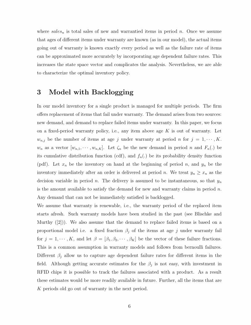
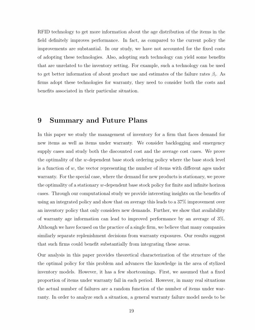
8.1 Cost Improvement over the Current Policy

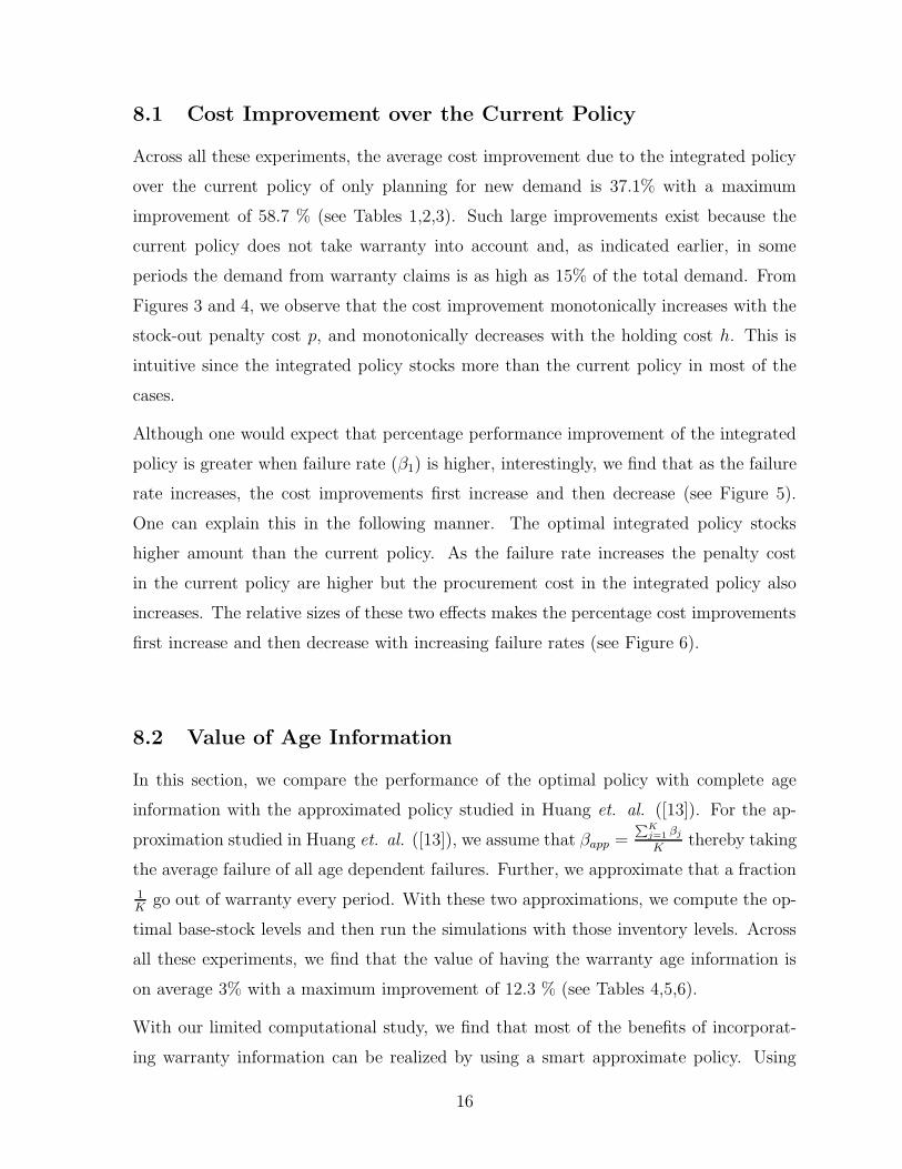
Across all these experiments, the average cost improvement due to the integrated policy

over the current policy of only planning for new demand is 37.1% with a maximum

improvement of 58.7 % (see Tables 1,2,3). Such large improvements exist because the

current policy does not take warranty into account and, as indicated earlier, in some

periods the demand from warranty claims is as high as 15% of the total demand. From

Figures 3 and 4, we observe that the cost improvement monotonically increases with the

stock-out penalty cost p, and monotonically decreases with the holding cost h. This is

intuitive since the integrated policy stocks more than the current policy in most of the

cases.

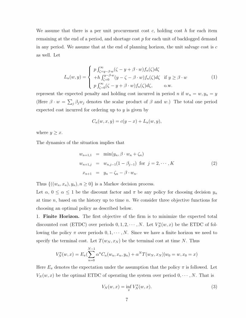
Although one would expect that percentage performance improvement of the integrated

policy is greater when failure rate (β1) is higher, interestingly, we find that as the failure

rate increases, the cost improvements first increase and then decrease (see Figure 5).

One can explain this in the following manner. The optimal integrated policy stocks

higher amount than the current policy. As the failure rate increases the penalty cost

in the current policy are higher but the procurement cost in the integrated policy also

increases. The relative sizes of these two effects makes the percentage cost improvements

first increase and then decrease with increasing failure rates (see Figure 6).

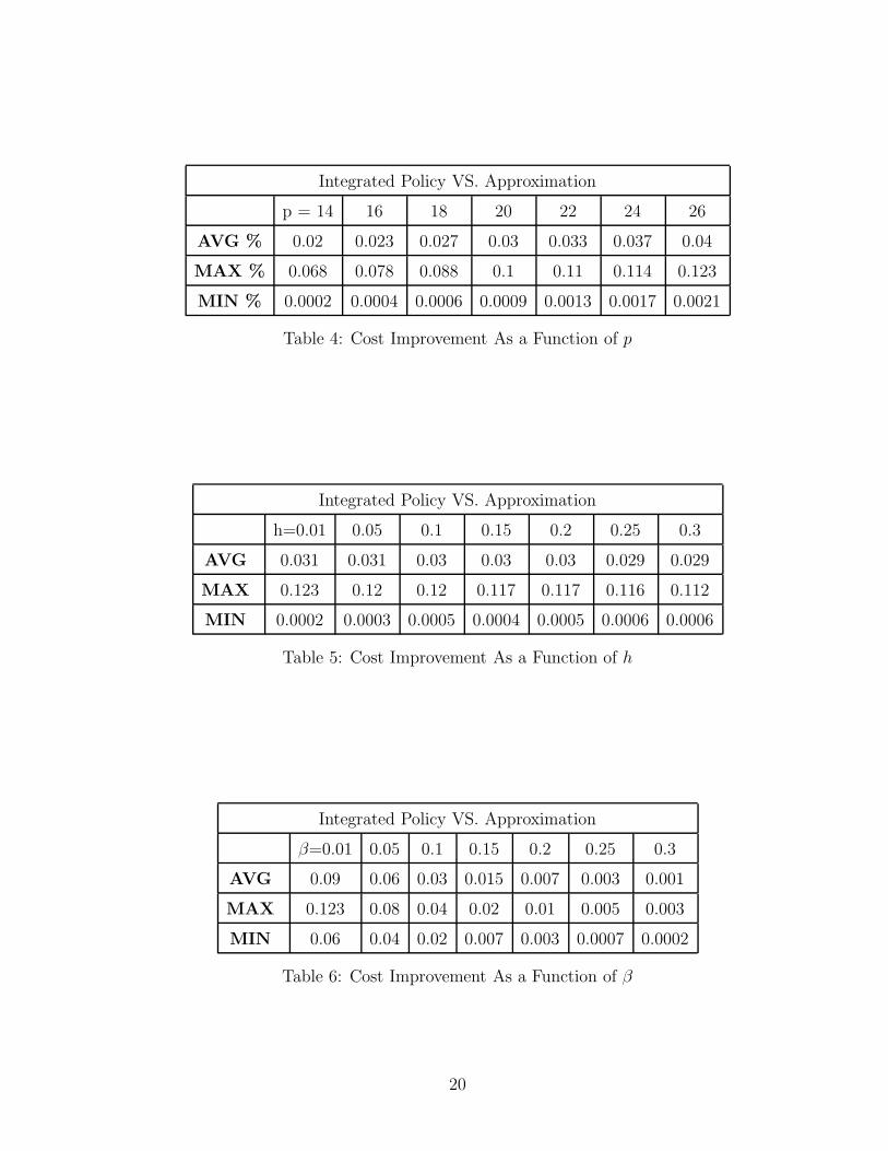
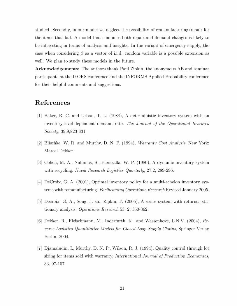
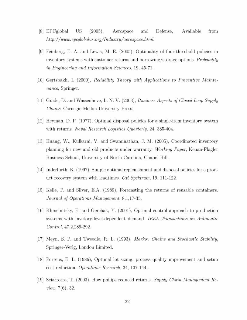
8.2 Value of Age Information

In this section, we compare the performance of the optimal policy with complete age

information with the approximated policy studied in Huang et. al. ([13]). For the ap-

proximation studied in Huang et. al. ([13]), we assume that βapp =PK

j=1 βj

Kthereby taking

the average failure of all age dependent failures. Further, we approximate that a fraction

1K

go out of warranty every period. With these two approximations, we compute the op-

timal base-stock levels and then run the simulations with those inventory levels. Across

all these experiments, we find that the value of having the warranty age information is

on average 3% with a maximum improvement of 12.3 % (see Tables 4,5,6).

With our limited computational study, we find that most of the benefits of incorporat-

ing warranty information can be realized by using a smart approximate policy. Using

16

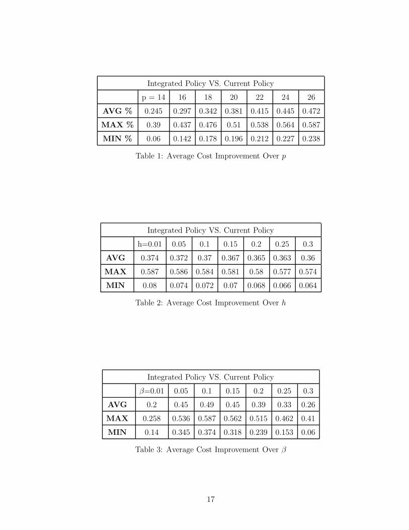
Integrated Policy VS. Current Policy

p = 14 16 18 20 22 24 26

AVG % 0.245 0.297 0.342 0.381 0.415 0.445 0.472

MAX % 0.39 0.437 0.476 0.51 0.538 0.564 0.587

MIN % 0.06 0.142 0.178 0.196 0.212 0.227 0.238

Table 1: Average Cost Improvement Over p

Integrated Policy VS. Current Policy

h=0.01 0.05 0.1 0.15 0.2 0.25 0.3

AVG 0.374 0.372 0.37 0.367 0.365 0.363 0.36

MAX 0.587 0.586 0.584 0.581 0.58 0.577 0.574

MIN 0.08 0.074 0.072 0.07 0.068 0.066 0.064

Table 2: Average Cost Improvement Over h

Integrated Policy VS. Current Policy

β=0.01 0.05 0.1 0.15 0.2 0.25 0.3

AVG 0.2 0.45 0.49 0.45 0.39 0.33 0.26

MAX 0.258 0.536 0.587 0.562 0.515 0.462 0.41

MIN 0.14 0.345 0.374 0.318 0.239 0.153 0.06

Table 3: Average Cost Improvement Over β

17

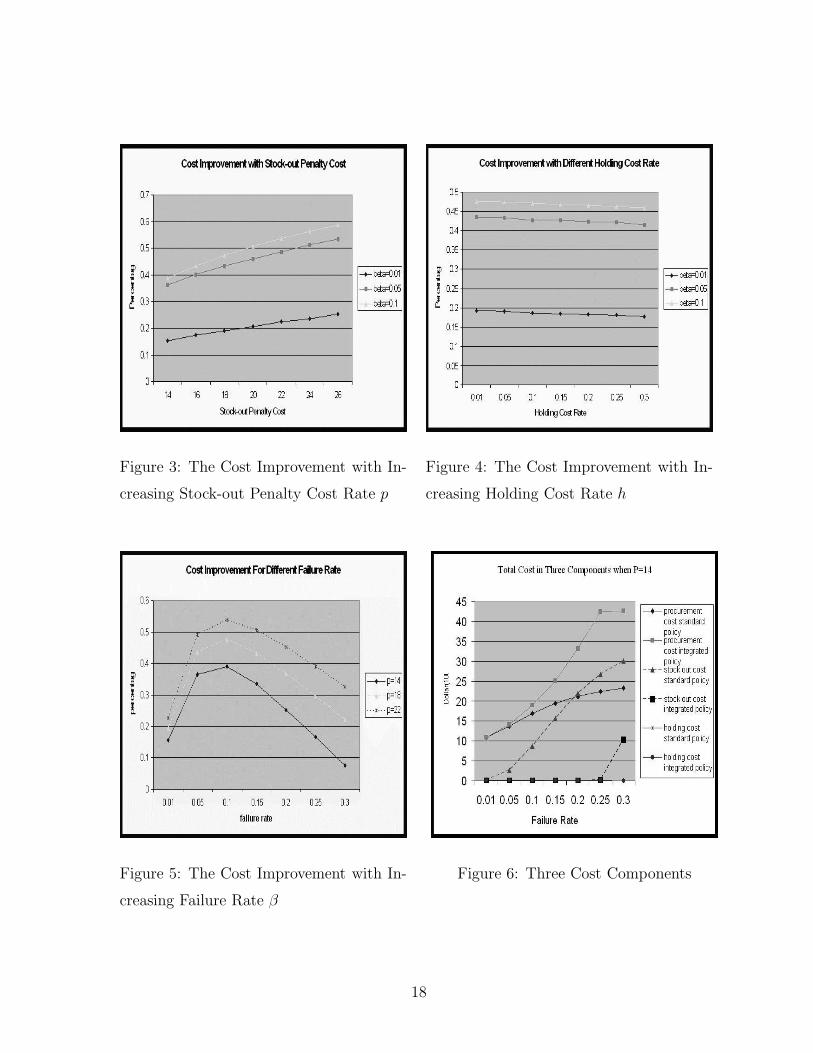
Figure 3: The Cost Improvement with In-

creasing Stock-out Penalty Cost Rate p

Figure 4: The Cost Improvement with In-

creasing Holding Cost Rate h

Figure 5: The Cost Improvement with In-

creasing Failure Rate β

Figure 6: Three Cost Components

18

RFID technology to get more information about the age distribution of the items in the

field definitely improves performance. In fact, as compared to the current policy the

improvements are substantial. In our study, we have not accounted for the fixed costs

of adopting these technologies. Also, adopting such technology can yield some benefits

that are unrelated to the inventory setting. For example, such a technology can be used

to get better information of about product use and estimates of the failure rates βi. As

firms adopt these technologies for warranty, they need to consider both the costs and

benefits associated in their particular situation.

9 Summary and Future Plans

In this paper we study the management of inventory for a firm that faces demand for

new items as well as items under warranty. We consider backlogging and emergency

supply cases and study both the discounted cost and the average cost cases. We prove

the optimality of the w-dependent base stock ordering policy where the base stock level

is a function of w, the vector representing the number of items with different ages under

warranty. For the special case, where the demand for new products is stationary, we prove

the optimality of a stationary w-dependent base stock policy for finite and infinite horizon

cases. Through our computational study we provide interesting insights on the benefits of

using an integrated policy and show that on average this leads to a 37% improvement over

an inventory policy that only considers new demands. Further, we show that availability

of warranty age information can lead to improved performance by an average of 3%.

Although we have focused on the practice of a single firm, we believe that many companies

similarly separate replenishment decisions from warranty exposures. Our results suggest

that such firms could benefit substantially from integrating these areas.

Our analysis in this paper provides theoretical characterization of the structure of the

the optimal policy for this problem and advances the knowledge in the area of stylized

inventory models. However, it has a few shortcomings. First, we assumed that a fixed

proportion of items under warranty fail in each period. However, in many real situations

the actual number of failures are a random function of the number of items under war-

ranty. In order to analyze such a situation, a general warranty failure model needs to be

19

Integrated Policy VS. Approximation

p = 14 16 18 20 22 24 26

AVG % 0.02 0.023 0.027 0.03 0.033 0.037 0.04

MAX % 0.068 0.078 0.088 0.1 0.11 0.114 0.123

MIN % 0.0002 0.0004 0.0006 0.0009 0.0013 0.0017 0.0021

Table 4: Cost Improvement As a Function of p

Integrated Policy VS. Approximation

h=0.01 0.05 0.1 0.15 0.2 0.25 0.3

AVG 0.031 0.031 0.03 0.03 0.03 0.029 0.029

MAX 0.123 0.12 0.12 0.117 0.117 0.116 0.112

MIN 0.0002 0.0003 0.0005 0.0004 0.0005 0.0006 0.0006

Table 5: Cost Improvement As a Function of h

Integrated Policy VS. Approximation

β=0.01 0.05 0.1 0.15 0.2 0.25 0.3

AVG 0.09 0.06 0.03 0.015 0.007 0.003 0.001

MAX 0.123 0.08 0.04 0.02 0.01 0.005 0.003

MIN 0.06 0.04 0.02 0.007 0.003 0.0007 0.0002

Table 6: Cost Improvement As a Function of β

20

studied. Secondly, in our model we neglect the possibility of remanufacturing/repair for

the items that fail. A model that combines both repair and demand changes is likely to

be interesting in terms of analysis and insights. In the variant of emergency supply, the

case when considering β as a vector of i.i.d. random variable is a possible extension as

well. We plan to study these models in the future.

Acknowledgements: The authors thank Paul Zipkin, the anonymous AE and seminar

participants at the IFORS conference and the INFORMS Applied Probability conference

for their helpful comments and suggestions.

References

[1] Baker, R. C. and Urban, T. L. (1988), A deterministic inventory system with an

inventory-level-dependent demand rate. The Journal of the Operational Research

Society, 39,9,823-831.

[2] Blischke, W. R. and Murthy, D. N. P. (1994), Warranty Cost Analysis, New York:

Marcel Dekker.

[3] Cohen, M. A., Nahmias, S., Pierskalla, W. P. (1980), A dynamic inventory system

with recycling. Naval Research Logistics Quarterly, 27,2, 289-296.

[4] DeCroix, G. A. (2001), Optimal inventory policy for a multi-echelon inventory sys-

tems with remanufacturing. Forthcoming Operations Research Revised January 2005.

[5] Decroix, G. A., Song, J. sh., Zipkin, P. (2005), A series system with returns: sta-

tionary analysis. Operations Research 53, 2, 350-362.

[6] Dekker, R., Fleischmann, M., Inderfurth, K., and Wassenhove, L.N.V. (2004), Re-

verse Logistics-Quantitative Models for Closed-Loop Supply Chains, Springer-Verlag

Berlin, 2004.

[7] Djamaludin, I., Murthy, D. N. P., Wilson, R. J. (1994), Quality control through lot

sizing for items sold with warranty, International Journal of Production Economics,

33, 97-107.

21

[8] EPCglobal US (2005), Aerospace and Defense, Available from

http://www.epcglobalus.org/Industry/aerospace.html.

[9] Feinberg, E. A. and Lewis, M. E. (2005), Optimality of four-threshold policies in

inventory systems with customer returns and borrowing/storage options. Probability

in Engineering and Information Sciences, 19, 45-71.

[10] Gertsbakh, I. (2000), Reliability Theory with Applications to Preventive Mainte-

nance, Springer.

[11] Guide, D. and Wassenhove, L. N. V. (2003), Business Aspects of Closed Loop Supply

Chains, Carnegie Mellon University Press.

[12] Heyman, D. P. (1977), Optimal disposal policies for a single-item inventory system

with returns. Naval Research Logistics Quarterly, 24, 385-404.

[13] Huang, W., Kulkarni, V. and Swaminathan, J. M. (2005), Coordinated inventory

planning for new and old products under warranty, Working Paper, Kenan-Flagler

Business School, University of North Carolina, Chapel Hill.

[14] Inderfurth, K. (1997), Simple optimal replenishment and disposal policies for a prod-

uct recovery system with leadtimes. OR Spektrum, 19, 111-122.

[15] Kelle, P. and Silver, E.A. (1989), Forecasting the returns of reusable containers.

Journal of Operations Management, 8,1,17-35.

[16] Khmelnitsky, E. and Gerchak, Y. (2001), Optimal control approach to production

systems with invetory-level-dependent demand. IEEE Transactions on Automatic

Control, 47,2,289-292.

[17] Meyn, S. P. and Tweedie, R. L. (1993), Markov Chains and Stochastic Stability,

Springer-Verlg, London Limited.

[18] Porteus, E. L. (1986), Optimal lot sizing, process quality improvement and setup

cost reduction. Operations Research, 34, 137-144 .

[19] Sciarrotta, T. (2003), How philips reduced returns. Supply Chain Management Re-

view, 7(6), 32.

22

[20] Simpson, V. P. (1978), Optimum solution structure for a repairable inventory prob-

lem. Operations Research, 26,2, 270-281.

[21] Swaminathan, J. M. and Tayur, S. R. (2003), Tactical Planning Models for Sup-

ply Chain Management. OR/MS Handbook on Supply Chain Management: Design,

Coordination and Operation, Elvesier Publishers, 423-456.

[22] Wang, Ch. H. and Sheu, Sh. h. (2003), Optimal lot sizing for products sold under

rree-repair warranty, European Journal of Operational Research, 149,131-141.

[23] Yuan, X. M. and Cheung, K. L. (1998), Modeling returns of merchandise in an

inventory system. Operations Research Spektrum, 20,3,147-154.

[24] Zipkin, P. (2000), Foundations of Inventory Management, McGraw Hill.

23

10 Appendix: Proofs

Proof of Proposition 1:

From the definition of mi, i = 1, · · · , K, we get

m1 = cβ1 + αβ1m1 + α(1 − β1)m2

m2 = cβ2 + αβ2m1 + α(1 − β2)m3

·

·

mK = cβK + αβKm1

Recursive substitution yields

mK = cβK + θKm1

mi = θic + αθim1 for i = K − 1, · · · , 1

where

θi =K

∑

j=i

αj−icβjΠj−1d=i (1 − βd) for i = 1, · · · , K.

Solving the above equations, we get

m1 =cθ1

1 − αθ1

mi = θic + αθim1 for i = 2, · · · , K

Proof of Theorem 1:

We will prove the above theorem using backward induction through two claims.

Claim 1: (i), (ii), and (iii) hold for N − 1.

24

Proof: Using the terminal cost function of Equation (5) we get

GN−1,N(w, y)

= cy + αLN−1(w, y)

+ α

∫ y−β·w

0

[m1(ζ + β · w) + m2w2 + · · ·+ mKwK − c(y − β · w − ζ)]fN−1(ζ)dζ

+ α

∫ ∞

y−β·w

[ym1 + m2w2 + · · ·+ mKwK − c(y − β · w − ζ)]fN−1(ζ)dζ

= cy + αLN−1(w, y) + αm2w2 + · · · + αmKwK − αc(y − β · w)

+ αcµN−1 + α

∫ y−β·w

0

(ζ + β · w)m1fN−1(ζ)dζ + α

∫ ∞

y−β·w

ym1fN−1(ζ)dζ

= c(1 − α)y + αLn−1(w, y) + αm2w2 + · · · + αmKwK

− αc(y − β · w) + α(µ + β · w)m1 + αcµN−1

where

LN−1(w, y) = h

∫ y−β·w

0

(y − β · w − ζ)fN−1(ζ)dζ

+(p − m1)

∫ ∞

y−β·w

(β · w + ζ − y)fN−1(ζ)dζ.

It is easy to show y = SN−1(w) = β ·w+F−1N−1(

p−c(1−α)p+h

) minimizes GN−1,N(w, y). Hence,

GN−1,N(w, y) increases with respect to y, when y ≥ SN−1(w). Therefore, we get

VN−1,N(w, x) =

GN−1,N(w, SN−1(w)) − cx if x ≤ SN−1(w)

GN−1,N(w, x) − cx o.w.

Now

GN−1,N(w, SN−1(w))

= c(1 − α)(β · w + F−1N−1(

p − c(1 − α)

p + h)) + αLN−1(w, SN−1(w))

+ w1(cβ1 + α(1 − β1)m2 + αβ1m1) + · · · + wK−1(cβK−1 + α(1 − βK−1)mK + αβK−1m1)

+ wK(cβK + αβKm1) + α(c + m1)µN−1

= m · w + α(m1 + c)µN−1 + c(1 − α)F−1N−1(

p − c(1 − α)

p + h) + αLN−1(w, SN−1(w)).

This yields

VN−1,N(w, x) = m · w − cx + ∆N−1

+

0 if x ≤ SN−1(w)

GN−1,N (w, x) − GN−1,N(w, SN−1(w)) o.w.

= m · w − cx + ∆N−1 + HN−1(w, x).

25

We also have

∂

∂y

∫ τN−1(w,y)

0

HN−1(w, x)fN−2(ζ)dζ

=∂

∂y

∫ τN−1(w,y)

0

[GN−1,N(w, x) − GN−1,N(w, SN−1(w))]fN−2(ζ)dζ

=

∫ τN−1(w,y)

0

G2N−1,N(w, x)fN−2(ζ)dζ

where the superscript 2 indicates partial derivative with respect to the second argument.

Since SN−1(w) minimizes GN−1,N(w, y) we can use the definition of HN−1(w, y) to get

{y : G2N−1,N(w, x) > 0} = {y : HN−1(w, x) > 0}.

From the assumption in Equation (9), we get SN−2(w) ≤ SN−1(w) + β · w. This proves

the quantity in Equation (13) is nonnegative when y ≥ SN−2(w).

Claim 2: If (i), (ii) and (iii) of Theorem 1 hold for n ≤ N − 1, then they hold for n− 1.

Proof: The induction hypothesis implies that we have

Gn,N(w, y) = c(1 − α)y + αLn(w, y) + (α∆n+1 + · · ·+ αn−1∆N )

+ (m · w) + α(m1 + c)µn + α

∫ ∞

0

Hn+1(w, x)fn(ζ)dζ.

Now, y = Sn(w) minimizes Gn,N(w, y), and Gn,N(w, y) increases with respect to y, when

y ≥ Sn(w). Also,∫ ∞

0Hn(w, x)fn−1(ζ)dζ is an increasing function of y when y ≥ Sn−1(w).

Then

Gn,N(w, Sn(w)) = (α∆n+1 + · · ·+ αn−1∆N) + (m · w) + α(m1 + c)µn

+ c(1 − α)Sn(w) + αLn(w, Sn(w))

= m · w + (∆n + · · ·+ αn−1∆N)

and correspondingly

Vn,N(w, x) = m · w − cx + (∆n + · · ·+ αn−1∆N)

+

0 if x ≤ Sn(w)

Gn,N(w, x) − Gn,N(w, Sn(w)) o.w.

26

Therefore from the DP recursion in Equation (4) we get

Gn−1,N(w, y) = cy + αLn−1(w, y)

+ α

∫ y−β·w

0

Vn,N(ζ + β · w, w2, · · · , wK, y − β · w − ζ)fn−1(ζ)dζ

+ α

∫ ∞

y−β·w

Vn,N(y, w2, · · · , wK, y − β · w − ζ)fn−1(ζ)dζ

= c(1 − α)y + αLn−1(w, y) + (α∆n + · · ·+ αn∆1) + m · w

+ α(m1 + c)µn−1 + α

∫ ∞

0

H(w, x)fn−1(ζ)dζ

which implies that (i) holds for n − 1. It is easy to see that y = Sn−1(w) minimizes

c(1 − α)y + αLn−1(w, y). The assumption (9) implies that

F−1n−1(

p − c(1 − α)

p + h) ≤ F−1

n (p − c(1 − α)

p + h)

which shows that τn(w, Sn−1(w)) < 0. This proves that

∫ τn(w,Sn−1(w))

0

Hn(w, Sn−1(w) − β · w − ζ)fn−1(ζ)dζ = 0.

Thus y = Sn−1(w) minimizes Gn−1,N(w, y). Hence, Gn−1,N(w, y) increases with respect

to y when y ≥ Sn−1(w). Furthermore, we have

∂

∂y

∫

∞

0

Hn−1(w, x)fn−2(ζ)dζ

=∂

∂y

∫ τn−1(w,y)

0

Hn−1(ζ + β · w, w2, · · · , wK , y − β · w − ζ)fn−2(ζ)dζ

=∂

∂y

∫ τn−1(w,y)

0

Gn−1,N (ζ + β · w, w2, · · · , wK , y − βw − ζ)fn−2(ζ)dζ

−∂

∂y

∫ τn−1(w,y)

0

Gn−1,N (ζ + β · w, w2, · · · , wK , Sn−1(ζ + β · w, w2, · · · , wK))fn−2(ζ)dζ

=

∫ τn−1(w,y)

0

G2n−1,N (ζ + β · w, w2, · · · , wK , y − β · w − ζ)fn−2(ζ)dζ

which is nonnegative when y ≥ Sn−2(w), since Gn−1,N(w, y) increases with respect to y

when y ≥ Sn−1(w). Hence

{y : G2n−1,N(w, y − β · w − ζ) > 0} = {y : Hn−1(w, y − β · w − ζ) > 0}

and

τn−1(w, Sn−2(w)) ≤ 0.

27

Thus (ii) holds for n − 1. This implies that the base stock level policy, which orders

up to Sn−1(w), is optimal for the discounted cost function over n − 1, n, · · · , N periods.

Clearly, we get

Gn−1,N(w, Sn−1(w)) = m · w + (∆n−1 + · · ·+ αn∆N ).

Therefore,

Vn−1,N(w, x) = m · w − cx + (∆n−1 + · · ·+ αn∆N)

+

0 if x ≤ Sn−1(w)

Gn−1,N(w, x) − Gn−1,N(w, Sn−1(w)) o.w.

which implies (iii) holds for n − 1. The theorem 1 follows from this.

Proof of Theorem 2:

From Equation (2) we get

wn+1,1 ≤ β · wn + ζn

wn+1,j = wn,j−1(1 − βj−1) for j = 2, · · · , K.

This can be written in matrix form as

wn+1 ≤ wnP + ζn,

where

P =

β1 (1 − β1) 0 · · · 0

β2 0 (1 − β2) · · · 0...

......

... · · ·...

βK 0 0 · · · 0

.

Letting e1 = [1, 0, · · · , 0] and taking expectations on both sides of the above inequality,

we get

Eπ∗(wn+1) ≤ Eπ∗(wn)P + µe1.

Iterating the above, we get

Eπ∗(wN) ≤ w0PN + µe1(I + P + · · ·+ P N−1)

≤ wP N + µe1(I − P )−1.

28

The effect of the initial inventory x0 = x is to increase the above right hand side at most

by x. Also E(xN ) ≥ −µ. Combining the above arguments we get that

Eπ∗(T (wN , xN)|w0 = w, x0 = x) = Eπ∗(m · wN − cxN |w0 = w, x0 = x)

≤ m · [(wP N) + µe1(I − P )−1] + cµ.

Since P is a sub-stochastic irreducible matrix,

limN→∞

P N = 0.

Hence,

limN→∞

αNEπ∗(T (wN , xN )|w0 = w, x0 = x) = 0.

Hence, it follows that

limN→∞

VN(w, x) = limN→∞

V π∗

N (w, x) = V (w, x),

and

limN→∞

V π∗

N (w, x) = V π∗

(w, x) = V (w, x).

That is, π∗ is optimal for the infinite horizon discounted cost case.

Proof of Proposition 2:

From the definition of the base stock policy and the equations (2),

xn+1 = max(xn, S(wn)) − β · wn − ζ

wn+1 = (min(β · wn + ζ, max(xn, S(wn))), wn,1(1 − β1), · · · , wn,K−1(1 − βK−1))

where S(wn) is shown as in the Equation (12). This implies that {(wn, xn), n ≥ 0} is

a DTMC. It is easy to show that it is irreducible and aperiodic. We prove the positive

recurrence by using the Foster’s Criterion (Meyn and Tweedie ([17]). Using the test

function υ(w, x) = |x| +∑K

j=1 wj we get

E(υ(wn+1, xn+1) − υ(wn, xn)|wn = w, xn = x)

= E(wn+1 + |xn+1||wn = w, xn = x) − w − |x|.

29

When x ≥ 0, we have

E(|xn+1| − xn|(wn = w, xn = x))

= E(|max(xn, S(wn)) − β · wn − ζn| − xn|(wn = w, xn = x))

≤

−β · w + µ if x ≥ S(w)

F−1( p

p+h) + µ − x, o.w.

≤ F−1(p

p + h) + µ − x,

and

E(wn+1 − wn|(wn = w, xn = x))

= E(min(β · wn + ζ, max(xn, S(wn))) +

K−1∑

j=1

wn,j(1 − βj) −

K∑

j=1

wn,j|(wn = w, xn = x))

=

E(min(β · wn + ζ, x) +∑K−1

j=1 wn,j(1 − βj) −∑K

j=1 wn,j|(wn = w, xn = x)) if x ≥ S(w)

E(min(β · wn + ζ, S(wn)) +∑K−1

j=1 wn,j(1 − βj) −∑K

j=1 wn,j|(wn = w, xn = x)), o.w.

≤

K∑

j=1

βjwj + µ +

K−1∑

j=1

wj(1 − βj) −

K∑

j=1

wj

= µ − wK(1 − βK).

Therefore

E(υ(wn+1, xn+1) − υ(wn, xn)|wn = w, xn = x)

= E(wn+1 + |xn+1| − wn − xn|wn = w, xn = x)

≤ F−1(p

p + h) + 2µ − wK(1 − βK) − x.

The last expression is < 0 if wK(1 − βK) + x > F−1( p

p+h) + 2µ.

When x ≤ 0, we have

E(|xn+1| − |xn||(wn = w, xn = x))

= E(|max(xn, S(wn)) − β · wn − ζn| + xn|(wn = w, xn = x))

≤ F−1(p

p + h) + µ + x

≤ 0 if x ≤ −µ − F−1(p

p + h),

30

and

E(wn+1 − wn|(wn = w, xn = x))

= E(min(β · wn + ζ, S(wn)) +K−1∑

j=1

wn,j(1 − βj) −K

∑

j=1

wn,j|(wn = w, xn = x))

≤ E(β · w + ζ +

K−1∑

j=1

wj(1 − βj) −

K∑

j=1

wj)

= µ − wK(1 − βK).

Therefore,

E(υ(wn+1, xn+1) − υ(wn, xn)|wn = w, xn = x)

= E(wn+1 + |xn+1| − wn + xn|wn = w, xn = x)

≤ F−1(p

p + h) + 2µ + x − wK(1 − βK)

The last expression is < 0 if −x + wK(1 − βK) > F−1( p

p+h) + 2µ.

Now, let A = {(w, x) : wK(1−βK)+ |x| ≤ F−1( p

p+h)+2µ} and note that A is a finite set.

Based on the above properties, we have shown that E(wn+1 + |xn+1| − wn − |xn||wn =

w, xn = x) < 0 if (w, x) /∈ A. Foster’s Criterion implies that {(wn, xn), n ≥ 0} is a

positive recurrent DTMC.

Proof of Proposition 3:

We get the total cost at period n as

E(Cn(wn, xn, yn)) = E(c(yn − xn) + h(yn − β · wn − ζn)+ + p(yn − β · wn − ζn)

−)

≤ E(c(yn − xn) + hyn + p(ζn + β · wn))

= E((c + h) max(xn, S(wn)) + p(ζn + β · wn) − cxn)

= (c + h)E(max(xn, S(wn))) − cE(xn) + pµ + pβ · E(wn).

When xn ≥ 0 then we can rewrite the above quantity as

E(Cn(wn, xn, yn)) ≤ (c + h)E(S(wn)) − cE(xn) + pµ + pβ · E(wn)

≤ (c + h)(β · E(wn) + F−1(p

p + h)) + pµ + pβ · E(wn)

≤ (c + h)F−1(p

p + h) + pµ + (c + h + p)β · (wP n + µe1(I − P )−1).

31

When xn ≤ 0 we have

E(Cn(wn, xn, yn)) ≤ (c + h)E(xn) − cE(xn) + pµ + pβ · E(wn)

≤ pµ + pβ · E(wn)

≤ pµ + pβ · (wP n + µe1(I − P )−1).

Hence, we get

limN→∞

E(Cn(wn, xn, yn)|w0 = w, x0 = x)

≤ (c + h)F−1(p

p + h) + pµ + (c + h + p)β · (wP N + µe1(I − P )−1)

< ∞.

Since (wn, xn) is an irreducible and positive recurrent DTMC, this shows that

limN→∞ E( 1N

∑N

n=0 Cn(wn, xn, yn)|w0 = w, x0 = x) exists.

Proof of Theorem 3:

Using the terminal cost in Equation (5) and using the argument in Theorem 3, we get

Eπ∗(T (wN , xN)|w0 = w, x0 = x) = Eπ∗(m · wN − cxN |w0 = w, x0 = x)

≤ m · (wP N + µe1(I − P )−1) + cµ.

Hence,

limN→∞

1

N + 1E(T (wN , xN )|w0 = w, x0 = x) = 0.

Proof of Theorem 4:

We prove the theorem using a series of claims by using induction.

Claim 1: GN−1,N(w, y) is convex with respect to y.

Proof:

From Equation (12), we get

GN−1,N(w, y) = cy + L(w, y)

and from the definition of L(w, y), the second order derivative of L(w, y) with respect to

y can be shown to be

L22(w, y) =∂2L(w, y)

∂y2= (p + h)f(y − β · w) > 0

32

This proves our claim 1.

Claim 2: If Gn,N(w, y) is convex with respect to y, then Vn,N(w, x) is convex with respect

to x.

Proof:

Let y = Sn(w) be the solution to

∂Gn,N (w, y)

∂y= 0.

The convexity of Gn,N(w, y) implies that the optimal policy at period n is order upto

Sn(w). Then

Vn,N(w, x) =

Gn,N(w, Sn(w)) − cx if x ≤ Sn(w)

Gn,N(w, x) − cx o.w.

We get the first order derivative of Vn,N(w, x) with respect to x as

V 2n,N(w, x) =

−c if x ≤ Sn(w)

G2n,N(w, x) − c o.w.

Since G2n,N(w, Sn(w)) = 0, V 2

n,N(w, x) is continuous at x = Sn(w), i.e., V 2n (w, Sn(w)+) =

V 2n (w, Sn(w)−) = −c. The second order derivative then can be shown to be

V 22n (w, x) =

0 if x ≤ Sn(w)

G22n (w, x) o.w.

Thus Vn(w, x) is convex with respect to w.

Claim 3: If Vn(w, x) is convex with respect to x, then Gn−1(w, y) is convex with respect

to y.

Proof: From the definition, we get

Gn−1(w, y)

= cy + L(w, y) + α

∫ y−β·w

0

Vn(w, y − ζ − β · w)f(ζ)dζ

+ α

∫ ∞

y−β·w

Vn(w, 0)f(ζ)dζ

33

The second order derivative of Gn−1(w, y) with respect to y can be shown to be

G22n−1(w, y) =

∂2

∂y2Gn−1(w, y)

=∂2

∂y2L(w, y) + α

∂2

∂y2

∫ ∞

0

Vn(w, (y − ζ − β · w)+)f(ζ)dζ

= L22(w, y) + α[

∫ y−β·w

0

V 22n (w, y − β · w − ζ)f(ζ)dζ

+V 2n (w, 0)f(y − β · w)].

From the Equation (13) and (13), the above quantity can be simplified as

G22n−1(w, y) = α

∫ y−β·w

0

V 22n (w, y − β · w − ζ)f(ζ)dζ

+ (p + h − αc)f(y − β · w)

≥ 0.

The above quantity is greater than zero by the assumptions, which implies that

Gn−1(w, y) is convex with respect to y.

Theorem 4 then follows by induction.

34