Embed Size (px)
Citation preview

Submitted to Operations Researchmanuscript OPRE-2014-03-142
Managing Inventories for Agricultural Products:The Optimal Selling Policies
Jim (Junmin) ShiDept. of Managerial Sciences, Robinson College of Business, Georgia State University, 35 Broad Street, Atlanta, GA 30303,
Yao ZhaoDept. of Supply Chain Management & Marketing Sciences, Rutgers Business School, Rutgers University, Newark, NJ 07102,
Rose B. KiwanukaAfrica Nazarene University, Nairobi, Kenya, [email protected]
The inventory control theory in the operations research and management literature is primarily concerned
about manufactured products, for which, the typical assumptions are ample external supplies and predictable
prices, and the decision is on how much to order or produce. Agricultural products, on the other hand,
are rarely studied in this literature but deserve an attention long overdue because of their unique features,
such as the limited and unpredictable supply, inelastic demand and thus highly unpredictable prices, and
a decision of how much to sell. Such features are considered in the agricultural economics literature which
provides insights and strategic guidelines but with limited structural results on the theory. Inspired by real-
life practice in the Kenya coffee industry, we consider a class of stochastic and dynamic inventory models
for storable agricultural products with random exogenous supply and price. We characterize the optimal
inventory (selling) policies for a variety of cost functions relevant in practice. In the cases of linear cost
functions, we derive closed-form expressions for the optimal policies and the optimal discounted profits. Our
theoretical advancement reveals additional insights and deepens the understanding of inventory management
for agricultural products. Applying the theory to practice, we show that making selling decisions judiciously
can significantly outperform the prevailing practice of selling-all regardless.
Key words : Agricultural products, inventory management, optimal selling policies, price fluctuation,
dynamic programming
1

Shi, Zhao and Kiwanuka: Agricultural Supply Chain2 Article submitted to Operations Research; manuscript no. OPRE-2014-03-142
1. Introduction
Many of the world’s poor still depend directly or indirectly on agricultural commodities for their
income, most of them are small-scale farmers in the third world countries. Taking coffee as an
example, an estimated 25 million small-scale farmers grow about 70% of the world’s coffee, and
about 125 million people in the world depend directly on coffee for their livelihoods (Oxfam 2001).
In the 1990s, exports by the 52 developing countries (Brazil, Vietnam, Colombia, Kenya, etc.) were
about U.S. $10-12 billion with the retail sales value, mainly in industrialized countries (the United
States, Germany, Japan, Italy, etc.) of about U.S. $30 billion (Osorio 2002). This makes coffee the
second most traded commodity in the world after petroleum.
1.1. The World Coffee Supply Chain
Coffee beans pass by many hands in various forms as they travel from farmers in the third-world
countries to consumers in the industrialized world (see Kiwanuka and Zhao 2009). Briefly, fresh
coffee cherries are harvested by farmers and then handed in, within 24 hours, to cooperatives for
the primary processing. The processed coffee beans, called the parchment coffee, are next passed to
millers for the secondary processing into green coffee beans, which have a long shelf-life (i.e., more
than ten years under proper storage conditions). The green coffee beans are then traded in the
international markets to importers, from where go to roasters before they finally reach retailers.
Coffee harvest (the supply) mainly depends on three factors: acreage of planting, weather and
farm input. The impact of acreage is not immediate as a coffee tree takes 5 to 6 years to mature.
Over the time, the world’s coffee harvest is increasing but significantly fluctuated due to unpre-
dictable weather conditions (Kiwanuka and Zhao 2009). The world’s coffee consumption, on the
other hand, grows steadily over time at an annual rate of about 0.5% (Daviron and Ponte 2006).
Generally, coffee consumption is insensitive to the price in the short term (Akiyama and Varangis
1990).
The random harvest (or supply) and the inelastic consumption of coffee have led to an extremely
fluctuated price for green coffee beans in the world commodity market; see Figure 1 for the inter-
national indicator price of coffee. For example, the sharp price spikes in 1975-77 and 1994-97 were

Shi, Zhao and Kiwanuka: Agricultural Supply ChainArticle submitted to Operations Research; manuscript no. OPRE-2014-03-142 3
caused by adverse weather conditions in Brazil. Indeed, frosts and droughts in Brazil where some
30% of the world’s coffee is grown have normally led to sudden upward movements in coffee prices
(Ponte 2002). Another significant factor on the price is the collapse of the International Coffee
Agreement (ICA) in 1989. ICA regulated coffee supply by setting quotas to exporting countries to
prevent price from falling below certain levels. Following the collapse of ICA, the price has been
driven primarily by market forces, and have fallen to a 30-year low in 1999-2001 which was below
the average production cost – causing the so-called “coffee crisis”.
Figure 1 Indicator price of coffee in the international market (in U.S. cents per lb.)
Source: International Coffee Organization: Statistics on Coffee.
The collapse of ICA and the following market liberalization put small-scale farmers world-wide
at a disadvantage. Specifically, the farmers face high transaction costs (e.g., variable and fixed
selling costs) with limited technical skills and market information. They (including their represent-
ing cooperatives) are price takers because they are too small to have leverage in the international
market. Finally, they must face the price fluctuations directly but lack of inventory and risk man-
agement tools. As a result, the prevailing practice in the developing countries is to sell-all harvest
regardless. Thus, the farmers cannot take advantage of an increase in price because no inventory is
kept. When the price drops, millions of small-scale farmers are driven out of business into poverty
and hunger.

Shi, Zhao and Kiwanuka: Agricultural Supply Chain4 Article submitted to Operations Research; manuscript no. OPRE-2014-03-142
1.2. Kenya Coffee Industry
Kenya’s coffee industry exemplifies the impact of price fluctuations on small-scale farmers. Due
to its ideal geographical location and weather, Kenya produces one of the finest types of coffee
(Colombian milds) in the world. Coffee is an important crop in Kenya contributing significantly
to the country’s export earnings and creates over 100,000 jobs plus supporting 5 million people
(Nyangito 2002). Statistically, 95% of Kenya’s annual harvest is exported, and Kenya’s share of
the world’s market on Colombian milds varies from 4.8% to 14% from 1990 to 2011.
There are two types of coffee farmers in Kenya: more than 700,000 small-scale farmers utilizing
just a few hectares of land, and about 3,400 estate (large-scale) farmers. Overall, the small-scale
farmers produce the majority of Kenya’s coffee with a better quality than the estate farmers because
of a better on-farm care and input. However, the small-scale farmers have been suffering the most
from the price fluctuations.
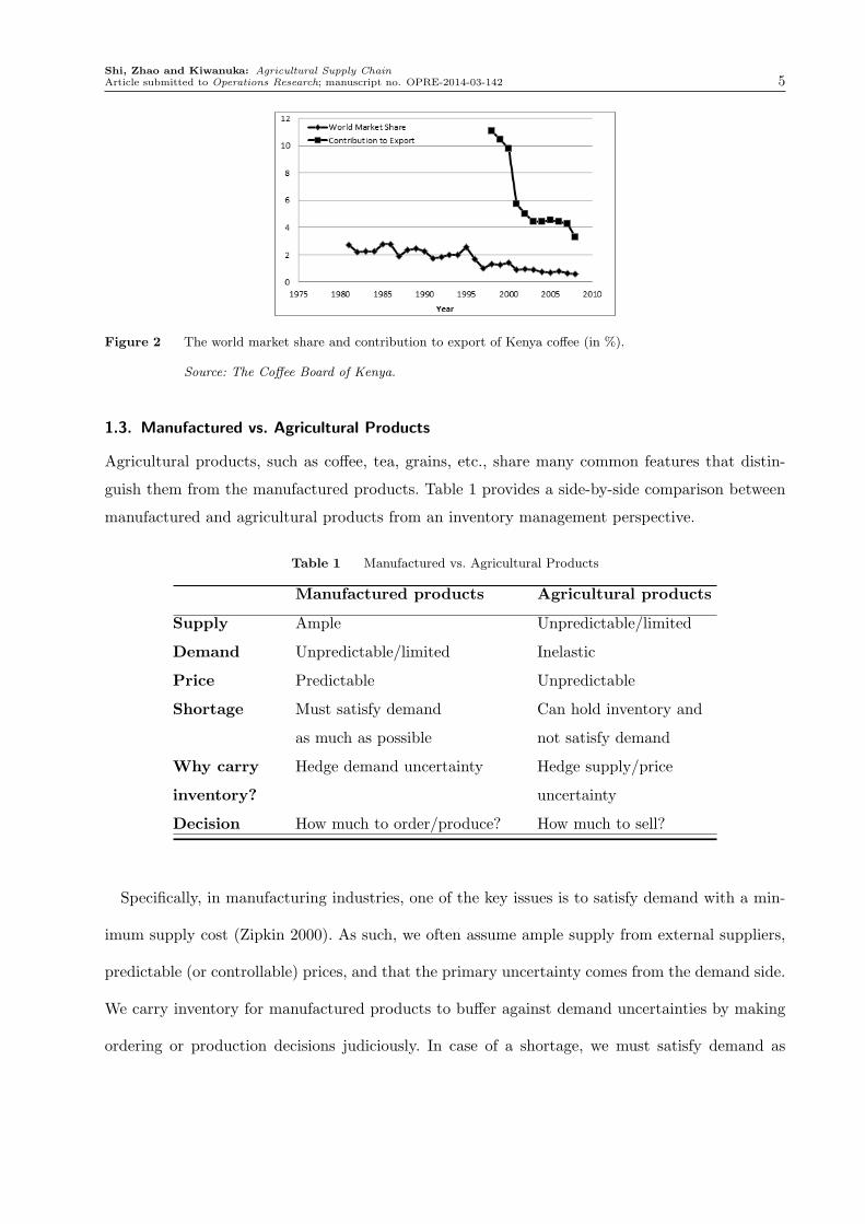
In the past two decades, Kenya’s coffee production has been largely declining (see Figure 2).
Coffee was the top foreign exchange earner in Kenya accounting for over 10% of the total export
earnings during the 1970s and the 1980s. In 1998, the sector contributed 11.07% to export earnings.
But since then, coffee production and export have been sharply declining, and in 2008, to the level
of 3.27%, making coffee the fourth in the rank of export earnings. Meanwhile, the world market
share of Kenya’s coffee has been decreasing from around 3% in the 1980s to 0.6% in 2008. The
decline of the coffee industry has a disastrous impact on the livelihood of coffee growers in Kenya as
well as the country’s economy. It is neither good for the international buyers and the consumers in
the industrialized world. To achieve the Millennium goal No. 1 of eradicating extreme hunger and
poverty, and to sustain the coffee industry in the long-run, we must improve small-scale farmers’
income. Clearly, many things can be done here, such as collective marketing to improve leverage,
and information and education to enhance visibility and productivity. In this paper, we develop
mathematical models and theory for the inventory management of agricultural products to improve
profitability.
Shi, Zhao and Kiwanuka: Agricultural Supply ChainArticle submitted to Operations Research; manuscript no. OPRE-2014-03-142 5
Figure 2 The world market share and contribution to export of Kenya coffee (in %).
Source: The Coffee Board of Kenya.
1.3. Manufactured vs. Agricultural Products
Agricultural products, such as coffee, tea, grains, etc., share many common features that distin-
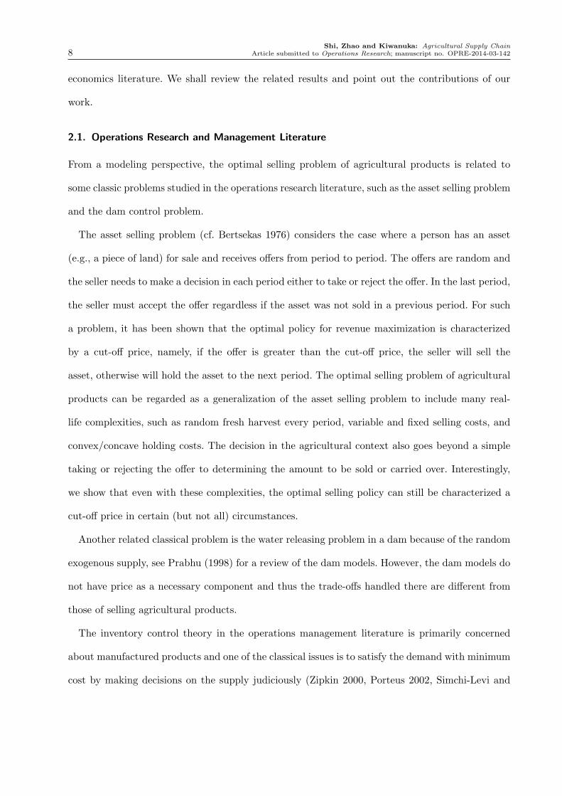
guish them from the manufactured products. Table 1 provides a side-by-side comparison between
manufactured and agricultural products from an inventory management perspective.
Table 1 Manufactured vs. Agricultural Products
Manufactured products Agricultural products
Supply Ample Unpredictable/limited
Demand Unpredictable/limited Inelastic
Price Predictable Unpredictable
Shortage Must satisfy demand Can hold inventory and
as much as possible not satisfy demand
Why carry Hedge demand uncertainty Hedge supply/price
inventory? uncertainty
Decision How much to order/produce? How much to sell?
Specifically, in manufacturing industries, one of the key issues is to satisfy demand with a min-
imum supply cost (Zipkin 2000). As such, we often assume ample supply from external suppliers,
predictable (or controllable) prices, and that the primary uncertainty comes from the demand side.
We carry inventory for manufactured products to buffer against demand uncertainties by making
ordering or production decisions judiciously. In case of a shortage, we must satisfy demand as

Shi, Zhao and Kiwanuka: Agricultural Supply Chain6 Article submitted to Operations Research; manuscript no. OPRE-2014-03-142
much as possible until we exhaust all available inventory. In contrast, the primary uncertainty of
an agricultural product may come from the supply side due to the unpredictable weather condi-
tions. Agricultural products satisfy the essential needs of people and thus the demand is generally
inelastic to prices. So, the price for an agricultural product is inherently random driven by unpre-
dictable and limited supplies. While it is unwise to hold inventory and shortage simultaneously
for a manufactured product, it is legitimate to do so for agricultural products if the price is not
right. Thus, we may carry inventory for agricultural products to buffer against supply and price
uncertainties by deciding, judiciously, how much to sell.
Intuitively, the selling decision must balance the following trade-off: (i) selling now, then we can
carry less inventory into the future but must accept the current price. (ii) Selling later, then we
have to carry more inventory but may get a better price in the future. Based on this intuition, a
simple strategy developed in the agricultural economics literature (e.g., Fackler and Livingstone
2002) says that “Agricultural producers with access to storage have flexibility in choosing the timing
and quantities of sales out of storage, e.g., a simple strategy considers whether the price is expected
to rise in the near future to cover the cost of storage (including the opportunity cost of capital).”
In this paper, we attempt to answer the following research questions:
1) How to manage inventories for agricultural products? Specifically, when to sell? How much to
sell? What is the impact?
2) How does the selling decision depend on transaction costs (holding, selling), price statistics, and
the planning horizon?
3) When does the simple strategy developed in the agricultural economics literature work? When
does it not work?
1.4. Results and Contributions
In this paper, we consider a class of stochastic and dynamic inventory models for agricultural
products with random exogenous supply and prices. The models are inspired and justified by an
empirical study of the real-life practice in the Kenya coffee industry. We characterize the optimal

Shi, Zhao and Kiwanuka: Agricultural Supply ChainArticle submitted to Operations Research; manuscript no. OPRE-2014-03-142 7
inventory (selling) policy for a variety of cost functions, such as linear or linear plus fixed cost for
selling, concave or convex cost for carrying inventory. For convex carrying cost and linear selling
cost functions, we show that the optimal policy is a selling-down-to policy that sells a portion of
the available inventory while retains the rest. Including a fixed selling cost shall change the optimal
policy to a “selling-down-to (S, s)” policy. Interestingly, for all other combinations of the cost
functions, the optimal policy is a selling-all-or-retaining-all policy although the critical thresholds
on price or inventory may differ. For linear cost functions, we further derive closed-form recursive
equations to calculate the optimal cut-off prices and the optimal discounted profit in a finite time
horizon. For the corresponding infinite horizon problem, we prove the convergence of the optimal
cut-off prices and discounted profits, and derive closed-form expressions for the limits. Finally, we
apply the theory to the empirical data and demonstrate the potential impact of the optimal policies
in the Kenya’s coffee industry.
This paper introduces the inventory management issues of agricultural products to the operations
research and management literature. As we shall show, sophisticated OR/OM models and tools,
such as stochastic dynamic programming, can significantly advance the knowledge and insights
previously unaware in the agricultural economics literature, and can make a significant impact on
practice - improving the livelihood for millions of farmers around the world and helping to sustain
the agricultural industries in the long run.
The remainder of this paper is organized as follows: we review the related literature in §2, which
is followed by an empirical study on the price and harvest processes of Kenya coffee in §3. In §4,
we present the mathematical model and the general theory on the optimal selling policy. In §5, we
analyze an important special case where the inventory holding cost is linear and derive closed-form
expressions and managerial insights. We conduct a numerical study to quantify the potential of
the optimal selling policies based on real-life data in §6, and conclude the paper in §7.
2. Literature Review
This paper is related to two large bodies of literature: inventory control theory in the operations
research and management literature, and post-harvest inventory management in the agricultural
Shi, Zhao and Kiwanuka: Agricultural Supply Chain8 Article submitted to Operations Research; manuscript no. OPRE-2014-03-142
economics literature. We shall review the related results and point out the contributions of our
work.
2.1. Operations Research and Management Literature
From a modeling perspective, the optimal selling problem of agricultural products is related to
some classic problems studied in the operations research literature, such as the asset selling problem
and the dam control problem.
The asset selling problem (cf. Bertsekas 1976) considers the case where a person has an asset
(e.g., a piece of land) for sale and receives offers from period to period. The offers are random and
the seller needs to make a decision in each period either to take or reject the offer. In the last period,
the seller must accept the offer regardless if the asset was not sold in a previous period. For such
a problem, it has been shown that the optimal policy for revenue maximization is characterized
by a cut-off price, namely, if the offer is greater than the cut-off price, the seller will sell the
asset, otherwise will hold the asset to the next period. The optimal selling problem of agricultural
products can be regarded as a generalization of the asset selling problem to include many real-
life complexities, such as random fresh harvest every period, variable and fixed selling costs, and
convex/concave holding costs. The decision in the agricultural context also goes beyond a simple
taking or rejecting the offer to determining the amount to be sold or carried over. Interestingly,
we show that even with these complexities, the optimal selling policy can still be characterized a
cut-off price in certain (but not all) circumstances.
Another related classical problem is the water releasing problem in a dam because of the random
exogenous supply, see Prabhu (1998) for a review of the dam models. However, the dam models do
not have price as a necessary component and thus the trade-offs handled there are different from
those of selling agricultural products.
The inventory control theory in the operations management literature is primarily concerned
about manufactured products and one of the classical issues is to satisfy the demand with minimum
cost by making decisions on the supply judiciously (Zipkin 2000, Porteus 2002, Simchi-Levi and

Shi, Zhao and Kiwanuka: Agricultural Supply ChainArticle submitted to Operations Research; manuscript no. OPRE-2014-03-142 9
Zhao 2011). This is consistent to the nature of manufactured products which can be cheaply and
massively produced and thus a failure to satisfy the demand often results in intolerable losses. The
optimal ordering and production policies of manufactured products are studied extensively in this
literature with many real-life complexities such as random yield or capacity (Yano and Lee 1995,
Wang and Gerchak 1996), supply disruptions (Tomlin 2006, Wang, Gilland and Tomlin 2010),
controllable price (Federgruen and Heching 1991, Chen and Simchi-Levi 2004), and releasing deci-
sions (Bhaskaran, Ramachandran and Semple 2010). This literature goes beyond order/production
decisions to analyze various sourcing strategies, innovative supply contracts, operational flexibility
and demand pooling strategies (e.g., component commonality), please see Huchzermeier and Cohen
(1996), Van Mieghem (1999, 2003, and 2007), Boyabatli and Toktay (2004), and the reference
therein.
Surprisingly, there is little work in the operations management literature on the inventory man-
agement of agricultural products thus far, to the best of our knowledge. However, one cannot simply
infer the models and results of manufactured products to agricultural products because the radical
difference of the latter (from the former) requires new models, methodologies and insights. One
of the main differences is that one can intentionally hold inventory of agricultural products from
satisfying the demand if the price is not right. That is, the selling decision is at least as important
as the planting (production) decision for the farmers and their cooperatives. For crops such as
coffee and tea, the supply is exogenous in the short term (due to the multiple years of time for
the trees to mature) driven primarily by unpredictable weather conditions. Thus, for these crops,
selling is likely the only decision relevant operationally. Another important difference lies in the
trade-off addressed by inventory control: for manufactured products, the trade-off typically centers
around inventory carrying cost vs. stockout cost; but for agricultural products, the trade-off is on
inventory carrying cost vs. a potentially higher price in the future. A comprehensive comparison
between manufactured and agricultural products can be found in Table 1.
More recently, the optimal selling policy has been studied in connection to the ordering policies
by Bhaskaran, Ramachandran and Semple (2010) in the operations management literature. This

Shi, Zhao and Kiwanuka: Agricultural Supply Chain10 Article submitted to Operations Research; manuscript no. OPRE-2014-03-142
paper considers manufactured products but assumes a convex ordering cost and the demand can
be rejected if the unit ordering cost exceeds the benefit of satisfying an additional demand. The
paper shows that the optimal ordering policy is an order-up-to policy dependent on the initial
inventory level and the optimal selling policy is to stop selling when backorders reach a critical
threshold. As typical in this literature, Bhaskaran, et al. (2010) assumes that supply is ample and
price is not a consideration. The trade-off studied in the paper is between a higher ordering cost
and losses of sales.
Despite the difference between manufactured and agricultural products, the optimal selling poli-
cies of the latter bear some resemblances to the optimal ordering policies of the former under
certain conditions. We shall explore and discuss these resemblances at length later in the paper.
The agriculture sector presents many operational challenges and is an important research area
from the perspective of social well-being, and thus has gained attentions from the operations
management literature in recent years, see, e.g., Kazaz and Webster (2011) and An, Cho and Tang
(2013). In particular, An, et al. (2013) study the impact of cooperatives and collective marketing
on producing cost, yield, brand awareness, supply chain consolidation and price uncertainty. Kazaz
and Webster (2011) study the agricultural industry under yield-dependent trading cost structure
in the presence of supply and demand uncertainty. To hedge supply uncertainty, they propose three
strategies: leasing farm space, free trading out/in materials in an open market, and pricing the
final product. It is shown that the yield-dependent unit purchasing cost has a significant impact
on the optimal decisions regarding the sale price and the production quantity. However, inventory
is not considered in these papers.
2.2. Agricultural Economics Literature
The agricultural economics literature has studied post-harvest inventory management since the
1950s when Gustafson (1958) introduces dynamic programming to problems of grain storage and
discusses the optimal stockpiling rules from a government perspective. The paper seeks the objective
of maximizing net benefit to the general public by evening out variations in year-to-year supplies.

Shi, Zhao and Kiwanuka: Agricultural Supply ChainArticle submitted to Operations Research; manuscript no. OPRE-2014-03-142 11
Random price fluctuation is not considered in this class of models. We refer to Wright (2001) for
a review of related follow-up works.
Another stream in this literature takes into account the price fluctuation from the institu-
tional/governmental sellers’ perspective. For instance, Alaouze, Sturgess and Watson (1978) studies
a dynamic programming model for Australian wheat assuming that Australia is a price taker with
a limited storage capacity. They solved the model numerically based on empirical data using value
iteration. Knapp (1982) generalizes Alaouze, et al. (1978) by considering trade and borrowing
options in the presence of foreign exchange issues between countries subject to fluctuations in
domestic harvests and world grain prices. For a simple case (two harvest levels and two prices),
they provide intuitions (but without a proof) for the optimal policy. Tronstad and Taylor (1991)
studies a risk-neutral dynamic model to make grain storage decisions and futures market transac-
tions by taking nonlinear tax issues into account. However, because of the large number of factors
considered in the model, the resulting decision rule is difficult to characterize and calculate.
The selling decisions have been studied in this literature for small-scale farmers. Berg (1987)
considers both risk-neutral and risk-averse farmers for grain carryover problems. Assuming risk
neutrality and i.i.d. price process, the paper studies the selling-all-or-retaining-all (SARA) policies
and provides a recursive procedure to calculate the best cut-off prices. For risk-averse farmers,
the paper shows that spreading sales over the crop season can be a better policy than the SARA
policy. Blakeslee (1997) considers a risk-averse model with a negative exponential utility function
for wheat storage, and uses Taylor-series to approximate the expected utility functions. Lai, Myers
and Hanson (2003) confirms the result of Berg (1987) that the policy of spreading sales out over
the crop season outperforms the SARA policy for risk averse farmers under a more general price
distribution.
For risk-neutral models, the only result to date on the optimal selling policy is obtained by
Fackler and Livingston (2002) which considers dynamic selling decisions in a continuous-time model
with linear profits. The price process is modeled by an one-factor Ito diffusion process. The paper
Shi, Zhao and Kiwanuka: Agricultural Supply Chain12 Article submitted to Operations Research; manuscript no. OPRE-2014-03-142
shows that the optimal policy is an SARA policy where the optimal cut-off price can be found by
solving a partial differential equation. For discrete models, it is not known what policy is optimal
even for the linear cost functions, let alone real-world complexities such as convex, concave, linear
plus fixed cost functions and storage capacity constraints. Although Berg (1987) studies the SARA
policy in discrete time, it does not show whether the policy is optimal among all possible policies.
Indeed, as we shall show in this paper, the SARA policy may not be optimal for some nonlinear
cost functions relevant in practice.
This paper contributes to this literature in several ways: (1) we broaden the scope of this lit-
erature by considering much more general cost functions (i.e., concave or convex carrying cost,
fixed selling cost) and price processes (e.g., Markovian) relevant in practice. (2) We advance the
inventory theory for agricultural products by characterizing the optimal selling policies for all
aforementioned cost functions and price processes in a risk-neutral discrete-time model. Interest-
ingly, we show that the popular selling-all-or-retaining-all policy is optimal not only for linear cost
functions but also for a wide-range of nonlinear cost functions under a general Markovian price
process. However, for convex cost functions, the optimal policy has a different structure, which is
of the type of selling-down-to (resembling the optimal ordering policy of manufactured products).
(3) For the well studied case of linear cost functions and independent price process, our closed-
form expressions for the optimal cut-off price in a finite time horizon simplify those of Berg (1987)
by directly connecting the prices in different periods without calculating the cost-to-go functions.
Our closed-form results for the optimal profit functions and for the infinite time horizon case are
new. (4) The theoretical advancement allow us to develop deeper insights and tell when the simple
insight of Fackler and Livingstone (2002, see §1.3) holds true and when it does not hold.
3. An Empirical Study
In this section, we conduct an empirical study on the price, harvest and export processes for Kenya
coffee which provides a basis to formulate the mathematic model in §4.

Shi, Zhao and Kiwanuka: Agricultural Supply ChainArticle submitted to Operations Research; manuscript no. OPRE-2014-03-142 13
3.1. Kenya Coffee Price Process
Kenya coffee is classified by the International Coffee Organization (ICO) as an Columbian Mild
and sold as such. We collect the monthly “Columbian Milds selling prices” published by ICO from
crop year 1991/92 to 2010/11. The price is in U.S. cents per lb. Because Kenya coffee has one
main harvest season each year, we average the monthly prices over a crop-year to obtain a series
of annual coffee prices.
A descriptive statistics shows that the price has a mean of 167.29 cents and a standard deviation
of 60.17 cents. To study the autocorrelation of the price process, we use a simple least-square
regression which yields the following model:
Pt−1 = 58.91+0.66Pt + ϵt,
where periods are backward indexed (such convention will be adopted throughout this paper), the
noise term ϵt has a mean of 0 and a standard deviation of 47.69, and the R-square is 0.405.
To further test the strength of the first-order auto-correlation, we use the Q-statistic introduced
by Box and Pierce (Pindyck and Rubinfeld 1998) to test the following:
H0: The first-order auto-correlation coefficient of the price process is zero.
H1: The first-order auto-correlation coefficient of the price process is NOT zero.
We shall reject the null hypothesis if the Q-statistic is greater than the critical 5-percent level
for a chi-square distribution. In our case, the Q-statistic is 7.41 and the critical value is 3.84, so we
reject the null hypothesis and conclude that the first-order auto-correlation coefficient of the coffee
price process is not zero at the 5-percent level of significance.
Now we estimate the probability distribution of the residuals ϵt. The descriptive statistics shows
that ϵt has a standard deviation of 47.69 cents. We further test the following:
H0: The residuals ϵt follow a normal distribution.
H1: The residuals ϵt do not follow a normal distribution.
Shi, Zhao and Kiwanuka: Agricultural Supply Chain14 Article submitted to Operations Research; manuscript no. OPRE-2014-03-142
We test these hypotheses using the Shapiro-Wilk Normality test (Ugarte, Militino and Arnholt
2008, pg 461) and the Jarque Bera test (Pindyck and Rubinfeld 1998, pg 47) at the 5-percent level
of significance. Our calculations show that the Shapiro-Wilk Normality test and Jarque Bera test
yield statistically insignificant p-values of 0.12 and 0.43 respectively. Therefore, we fail to reject
the null hypothesis at the 5-percent level of significance, and conclude that the residuals follow a
normal distribution.
3.2. Kenya Coffee Harvest Process
We collect the annual coffee harvest (production) data from the annual reports of the Coffee Board
of Kenya (CBK) for the crop years from 1991/92 to 2010/11. A descriptive statistics shows that
the annual harvest has a mean of 60,956 tons and a standard deviation of 21,567 tons. To study
the autocorrelation of the harvest data, we use a simple least-square regression which shows an
R-square of 0.221.
To further test the strength of the first-order auto-correlation in annual harvest data, we use the
Q-statistic by Box and Pierce (ibid) to test the following hypothesis.
H0: The first-order auto-correlation coefficient of annual harvest is zero.
H1: The first-order auto-correlation coefficient of annual harvest is NOT zero.
Similar to the price process, we shall reject the null hypothesis if the Q-statistic is greater than
the critical 5-percent level. In this case, the Q-statistic is 3.29 while the critical value is 3.84, so
we fail to reject the null hypothesis and conclude that the first-order auto-correlation coefficient
in the harvest process is zero. In addition to the Box and Pierce test, we use the Breusch-Pagan
and White Tests (Pindyck and Rubinfeld 1998) to test the above hypothesis. In our case, the test
statistic is 0.15 for the Breusch-Pagan and 3.60 for the White Test, each of which is less than the
critical value 3.84 at the 5 percent level. Hence, we fail to reject the null hypothesis and reach
the same conclusion. For each approach tried here, we also tested higher order auto-correlations
(e.g., the 2nd and 3rd) and obtain the same result. Based on these evidences, we can statistically
conclude that Kenya’s coffee harvests are independent across crop years.

Shi, Zhao and Kiwanuka: Agricultural Supply ChainArticle submitted to Operations Research; manuscript no. OPRE-2014-03-142 15
3.3. Coffee Price vs. Export
We now study the dependence between price and export for Kenya coffee. Our calculation shows
that the correlation coefficient between the annual price process and the annual export process is
as small as 0.20. To further test the strength of the correlation, we use the following hypothesis.
H0: The correlation coefficient between price and export is zero.
H1: The correlation coefficient between price and export is NOT zero.
We test this hypothesis using the Pearson product-moment correlation coefficient (Sheskin 2000,
pg 766). The decision rule is to reject the null hypothesis if the statistic is less than the critical value
of 0.414 at the 5-percent level of significance (for our case). Our calculation shows that the statistic
is 0.88 and thus we fail to reject the null hypothesis and conclude that there isn’t a significant
correlation between prices and exports for Kenya coffee.
We also test the correlations between coffee exports and the lagged coffee prices, but find them
statistically insignificant. From the foregoing statistical evidences, we can reasonably conclude that
the price for Kenya’s coffee is independent of Kenya’s export. Intuitively, this statement makes
sense as the price is determined by the total coffee traded in the world coffee market, of which
Kenya’s share is insignificant, 1-3%. This fact renders Kenya a price taker.
4. The Mathematic Model and General Theory
In this paper, we consider risk neutral sellers (e.g., growers or their cooperatives). Based on the
empirical study in §3, we make the following assumptions.
Assumption 1 a) The seller is a price taker, that is, the price is exogenous and independent of
the selling quantities over all seasons (periods).
b) The harvest in a season (period) is independent of the harvests in previous seasons (periods).
c) The price process is a Markov process in general; specifically, it can be auto-correlated and follow
an AR(1) process (for which the i.i.d. price process is a degenerated case).
Shi, Zhao and Kiwanuka: Agricultural Supply Chain16 Article submitted to Operations Research; manuscript no. OPRE-2014-03-142
Assumption 1 implies that the price does not depend on the selling quantity. We shall point out
that such a price taker assumption is often made in the literature, see, e.g., Alaouze, et al. (1978),
Berg (1987), and Fackler and Livingston (2002). In this paper we consider storable agricultural
products, e.g., green coffee beans, which can be held in inventory for an indefinite time under
proper conditions. For inventory carried over from one season to the next, a carrying cost incurs,
which includes storage cost, capital cost and interest, among others.
Following notational convention, we consider a finite planning horizon of T + 1 periods with a
backward index t = 0,1,2, ..., T where t = 0 denotes the last period and t = T denotes the first
period. For period t, we introduce the following notation:
• Pt: unit price after deducting tax and variable transaction cost, Pt > 0;
• pt: the realization of random variable Pt;
• Qt: newly available supply/harvest for sales (a random variable) in period t, Qt > 0;
• It: total inventory available for sales in period t;
• xt: the amount of sales made in period t;
• yt: inventory carried over from period t to t− 1;
• Ht(·): holding cost function for carrying inventory over from period t to t− 1;
• Kt: the fixed cost for sales transaction in period t;
• βt: the time discounted factor in period t.
The sequence of events can be described as follows: At the beginning of season t, the initial
inventory available for sales is yt+1. Then, the newly available supply/harvest for sales in this
season, Qt, is realized as qt. The seller updates the inventory as It = yt+1 + qt. Next, the market
price is observed as pt, the sales decision, xt, is made, and the leftover inventory (if any) yt = It−xt
is carried to the next period t− 1. In the sequel, we shall take yt as the decision variable in lieu of
xt. In the last season t= 0, we assume that all inventory available must be sold regardless of the
price p0.

Shi, Zhao and Kiwanuka: Agricultural Supply ChainArticle submitted to Operations Research; manuscript no. OPRE-2014-03-142 17
Let Vt(It, pt) be the optimal total discounted profit for the seller from season t to the end of
the planning horizon with an initial inventory It and a price pt observed in period t. We have the
following dynamic programming formulation:
Vt(It, pt) = pt · It + gt(It, pt); (1)
gt(It, pt) = max0≤yt≤It
{− δ(It − yt) ·Kt +Gt(yt, pt)
}; (2)
Gt(yt, pt) = −pt · yt −Ht(yt)+βt−1 ·E[Vt−1(yt +Qt−1, Pt−1)
∣∣∣∣pt], (3)
where the expectation in Eq. (3) is taken with respect to Qt−1 and Pt−1 conditioning on the
observed price pt in season t, and the function δ(x) = 1 if x > 0, δ(x) = 0 otherwise. For the last
period t= 0, V0(I0, p0) = I0 · p0 − δ(I0) ·K0.
In inventory models for manufactured products, the decision is typically on the order-
ing/production quantities that are determined before demand uncertainty is resolved. In contrast,
for agricultural products, the decision here is on the selling quantity that is determined after supply
and price uncertainties are resolved.
In what follows, we shall classify the model defined in Eqs. (1)-(3) by various cost structures
(for selling and inventory holding). In practice, a selling transaction may involve a fixed cost,
Kt > 0, representing shipping, loading/unloading, sampling and testing, as well as sales, general
and administrative (SG&A) expenses. While in some cases, such costs are covered by buyers and/or
sales agents, i.e., Kt = 0 for the seller; in other cases, the seller has to pay by itself, i.e., Kt > 0.
Inventory cost often includes storage cost and capital cost/interest as its two main components.
If the storage cost dominates, then the inventory carrying cost Ht(y) is likely concave due to
economies of scale in storage. Conversely, if the capital cost dominates, then Ht(y) is likely convex
due to the dis-economies of scale in capital cost and interest. In the sequel, we shall derive the
optimal dynamic selling policy for each of the four combinations of these cost structures: (i) Kt = 0
and concave holding cost, (ii) Kt > 0 and concave holding cost, (iii) Kt = 0 and convex holding
cost, and (iv) Kt > 0 and convex holding cost. More results are developed for the special case of
linear holding cost in §5.
Shi, Zhao and Kiwanuka: Agricultural Supply Chain18 Article submitted to Operations Research; manuscript no. OPRE-2014-03-142
4.1. Zero Fixed Selling Cost and Concave Holding Cost
In this section, we consider the dynamic program model by Eqs. (1)-(3) with Kt = 0 and concave
Ht(·) for all t. Thus, for each period t, the cost function, −ptyt −Ht(yt), is convex. We have the
following theorem (all proofs are included in Appendix).
Theorem 1 If Kt = 0 and Ht(y) is concave for all t= 1,2, ..., T , then,
(i) Vt(It, pt) is increasing and convex in It for all t.
(ii) The optimal selling policy is a selling-all-or-retaining-all policy. Specifically, there exists a
threshold quantity, Rt(pt)≥ 0, such that the optimal carry-over inventory
y∗t =
It, if It ≥Rt(pt);
0, o.w.
(4)
where
Rt(pt) = sup
{y≥ 0
∣∣∣∣ Gt(y, pt)≤Gt(0, pt)
}. (5)
In particular, Rt(pt) = +∞ if Gt(y, pt)<Gt(0, pt) for all y > 0; Rt(pt) = 0 if Gt(y, pt)>Gt(0, pt)
for all y > 0.
Theorem 1 states that there exists a price-dependent threshold, and it is optimal to sell all the
inventory if the inventory level is smaller than this threshold, otherwise, it is optimal to retain
all the inventory. This statement is consistent to the economies of scale in holding inventory, as
represented by the concavity of the inventory holding cost function Ht(·).
To study the sensitivity of the optimal profit function and the threshold value Rt(pt) with respect
to the price, we make the following assumption.
Assumption 2 The price process satisfies
Pt =At · ft(pt+1)+Bt, (6)
where the random variables At and Bt are independent of pt+1, At ≥ 0, and ft(p) is differentiable
and satisfies
0≤ f ′t(p) ·E[At]< 1. (7)
Shi, Zhao and Kiwanuka: Agricultural Supply ChainArticle submitted to Operations Research; manuscript no. OPRE-2014-03-142 19
Remark: The price process defined in Eq. (6) represents a general class of Markovian processes,
where the future price is stochastically increasing in the current price pt because f′t(p)> 0. However,
the price process is stable over time as f ′t(p)E[At] < 1. An example of this price process is the
AR(1) process, Pt = a · pt+1 + ϵ, where ft(p) = a · p, At = 1 and Bt = ϵ.
Proposition 1 If Kt = 0 and Ht(y) is concave all t = 1,2, ..., T , the following statements hold
under Assumption 2:
(i) Functions Vt(I, p) and Gt(y, p) satisfy
∂2Vt(I, p)
∂I · ∂p≤ 1;
∂2Gt(y, p)
∂y · ∂p≤ 0. (8)
(ii) The threshold Rt(pt) increases in pt.
Proposition 1 implies we should sell more and carry less inventory at a higher price pt, and vice
versa. This is true because the future price is more likely to drop by Assumption 2.
Proposition 2 If Kt = 0 and Ht(y) is concave for all t= 1,2, ..., T , then Vt(I, p) is increasing and
convex in p under Assumption 2 and the assumption of convex ft(p).
4.2. Positive Fixed Selling Cost and Concave Holding Cost
In this section, we assume that Kt > 0 and Ht(·) is concave for all t. Similar to §4.1, the cost
function, −ptyt −Ht(yt), is convex for all t. The following theorem characterizes the structure of
the optimal selling policy.
Theorem 2 If Kt > 0 and Ht(y) is concave for all t= 1,2, ..., T , then,
(i) Vt(It, pt) is increasing and convex in It for all t.
(ii) The optimal selling policy is an selling-all-or-retaining-all policy and there exists a pair of
thresholds 0≤ rt(pt)≤Rt(pt), such that the optimal carry-over inventory
y∗t =
0, if rt(pt)< It <Rt(pt);
It, o.w.
(9)
Shi, Zhao and Kiwanuka: Agricultural Supply Chain20 Article submitted to Operations Research; manuscript no. OPRE-2014-03-142
The two thresholds rt(pt)≤Rt(pt) are given by
rt(pt) = inf
{y≥ 0
∣∣∣∣ Gt(y, pt)≤Gt(0, pt)−Kt
}; (10)
Rt(pt) = sup
{y≥ 0
∣∣∣∣ Gt(y, pt)≤Gt(0, pt)−Kt
}, (11)
and Rt(pt) =+∞ if limy→∞
Gt(y, pt)<Gt(0, pt)−Kt.
Theorem 2 suggests to retain all inventory if It ≤ rt(pt). This is true because of the fixed selling
cost. Theorem 2 also suggests to retain all inventory if It ≥Rt(pt). This can be explained by the
economies of scale in holding inventory as in §4.1.
Similar to §4.1, we characterize the sensitivity of the thresholds as follows.
Proposition 3 If Kt > 0 and Ht(y) is concave for all t= 1,2, ..., T , then
(i) It is optimal to retain all inventory if and only if
Gt(0, pt)−miny>0
Gt(y, pt)<Kt. (12)
(ii) As Kt increases, rt(pt) increases and Rt(pt) decreases.
(iii) Under Assumption 2, rt(pt) decreases and Rt(pt) increases in pt.
Proposition 3 shows that it is less likely to sell all inventory if the fixed selling cost is greater, and
if the fixed selling cost is sufficiently large, it is optimal to retain all inventory. On the other hand,
it is more likely to sell all inventory if the observed price is higher.
4.3. Zero Fixed Selling Cost and Convex Holding Cost
In this section, we assume that Kt = 0 and Ht(·) is convex for all t. In this case, for each period t,
the cost function, −ptyt−Ht(yt), is concave. Theorem 3 provides structural results for the optimal
selling policy.
Theorem 3 If Kt = 0 and Ht(y) is convex for all t= 1,2, ..., T , then,
(i) Gt(yt, pt) is concave in yt for all t.
Shi, Zhao and Kiwanuka: Agricultural Supply ChainArticle submitted to Operations Research; manuscript no. OPRE-2014-03-142 21
(ii) Vt(It, pt) is increasing and concave in It for all t.
(iii) The optimal selling policy is an selling-down-to s policy, that is, there exists a threshold,
st(pt), such that the optimal carry-over inventory
y∗t =
st(pt), if It ≥ st(pt);
It, o.w.
(13)
where
st(pt) = argmaxy≥0
{Gt(y, pt)}, (14)
and st is independent of It and Qt.
Note that Theorem 3 holds for any V0(I0, p0) that is concave in I0. Intuitively, Theorem 3 shows
that it is optimal to sell down to st(pt) if the inventory level is above it; otherwise, retain all
inventory. We should point out that the selling-down-to policy for agricultural products resembles
the optimal order-up-to policies in inventory models for manufactured products although no simple
transformation can convert one model to the other.
Similar to previous sections, we characterize the sensitivity of the threshold as follows.
Proposition 4 If Kt = 0 and Ht(y) is convex for all t= 1,2, ..., T , the following statements hold
under Assumption 2:
(i) functions Vt(I, p) and Gt(y, p) satisfy
∂2Vt(I, p)
∂I · ∂p≤ 1;
∂2Gt(y, p)
∂y · ∂p≤ 0; (15)
(ii) the threshold st(pt) decreases in pt.
Proposition 4 indicates that it is more likely to sell more if the price pt is higher, and vice versa.
4.4. Positive Fixed Selling Cost and Convex Holding Cost
In this section, we assume that Kt > 0 and Ht(·) is convex for all t. Similar to §4.3, the cost
function, −ptyt −Ht(yt), is concave for all t. Theorem 4 characterizes the structure of the optimal
selling policy.
Shi, Zhao and Kiwanuka: Agricultural Supply Chain22 Article submitted to Operations Research; manuscript no. OPRE-2014-03-142
Theorem 4 If Kt > 0 and Ht(y) is convex for all t= 1,2, ..., T , and 0< βt ·Kt ≤Kt+1, then for
any given pt,
(i) gt(yt, pt) is Kt-concave in yt.
(ii) Vt(It, pt) is increasing and Kt-concave in It.
(iii) The optimal selling policy is an selling-down-to (S, s) policy, that is, in period t > 0, there
exists a pair of thresholds, 0≤ st(pt)<St(pt), such that the optimal carry-over inventory
y∗t =
st(pt), if It ≥ St(pt),
It, o.w.
(16)
where st(pt) = argmaxy≥0
{Gt(y, pt)} and
St(pt) = sup{y∣∣y > st, Gt(y, pt) =Gt(st, pt)−Kt
}. (17)
The thresholds St(pt) and st(pt) are independent of It and Qt.
Theorem 4 states that it is optimal to sell down to st if the inventory is greater than (or equal
to) St where St > st; otherwise, it is optimal to retain all inventory. Such a selling − down − to
(S, s) policy for agricultural products is analogous to the well-known (s, S) ordering policy for
manufactured products. The key difference is that the policies operate in the opposite direction:
ordering to stock up the inventory for manufactured products versus selling to deplete the inventory
for agricultural products.
5. Special Cases with Linear Holding Cost
In this section, we consider linear holding cost, that is, Ht(yt) = ht · yt for all t, where ht ≥ 0 is the
inventory carrying cost per unit per period. The dynamic programming model given by Eq. (3)
can be written as
Gt(yt, pt) =−(pt +ht) · yt +βt−1E[Vt−1(yt +Qt−1, Pt−1)|pt], (18)
where the equations for Vt(It, pt) and gt(It, pt) remain the same. Interestingly, linear inventory cost
allows us to derive much stronger results (e.g., closed-form recursive expressions) for the optimal
policy and discounted profit with or without a fixed selling cost.
Shi, Zhao and Kiwanuka: Agricultural Supply ChainArticle submitted to Operations Research; manuscript no. OPRE-2014-03-142 23
5.1. Zero Fixed Selling Cost
The following theorem provides closed-form recursive equations for the optimal selling policy and
discounted profit,
Theorem 5 If Kt = 0 and Ht(y) = ht · y for each period t, then
(i) the optimal selling policy is a selling-all-or-retaining-all policy characterized by a cut-off price,
p∗t , such that,
y∗t =
0, if pt ≥ p∗t ,
It, o.w.
(19)
where the cut-off price is recursively given by
p∗t ≡ p∗t (pt) = βt−1 ·E[max{Pt−1, p
∗t−1(Pt−1)}
∣∣∣∣pt]−ht, (20)
with p∗0 = 0.
(ii) The optimal discounted profit is explicitly given by
Vt(It, pt) =max{pt, p∗t} · It +t∑
s=1
βt,s ·(E[p∗s|pt] +hs
)·E[Qs−1] (21)
where for 0≤ s < t, βt,s = βt−1 ·βt−2 · · ·βs is the cumulative discount factor from period s to period
t (backward indexed).
Theorem 5 is consistent to Theorems 1 and 3. Specifically, for a linear Ht(·), we can show that,
depending on price pt, either Rt = 0 or Rt =+∞ in Theorem 1; either st = 0 or st =+∞ in Theorem
3. More precisely, st is determined by,
st =
0, if pt ≥ p∗t ,
+∞, o.w.
(22)
Theorem 5 provides rich insights on how to sell inventory for agricultural products. Let’s first
look at the 2nd last period. By Eq. (20) and the fact that p∗0 = 0, i.e., we sell all inventory in the
last period,
p∗1 = β0E[P0|p1]−h1. (23)
Shi, Zhao and Kiwanuka: Agricultural Supply Chain24 Article submitted to Operations Research; manuscript no. OPRE-2014-03-142
Thus it is optimal to sell all inventory in the 2nd last period if the price p1 is greater than or equal
to p∗1 which is the discounted expected price for the period 0 subtracting the inventory holding
cost. Furthermore, the cut-off price, p∗1, does not depend on the available inventory or the harvest.
This insight is nearly identical to the observation made by Fackler and Livingstone(2002), a simple
strategy considers whether the price is expected to rise in the near future to cover the cost of storage.
For periods prior to the 2nd last period, Eq. (20) indicates that the optimal cut-off price of one
period depends on the cut-off price of the next period. Hence, the simple observation of Fackler
and Livingstone(2002) does not work because we do not sell all inventory regardless of the price in
the next period, but only when the next periods cut-off price is met. Thus we must take the next
periods cut-off price into account in determining this period’s cut-off price.
Steady-State Analysis for I.I.D. Price Process. If prices in all periods are i.i.d. random
variables, i.e., Pt equals to P in distribution for all t, and the system parameters are stationary,
that is, ht = h, βt = β, ∀t, then we can obtain closed-form expressions for the optimal cut-off price
and the optimal discounted profit in steady state.
Proposition 5 If Pt = P in distribution, ht = h, βt = β for all t, then
(i) the cut-off prices satisfy
β ·E[P ]−h= p∗1 ≤ . . .≤ p∗t ≤ p∗t+1 → p∗,
where p∗ is uniquely determined by
p∗ = β ·E[max{P,p∗}]−h. (24)
(ii) If {Qt} are i.i.d. random variables, i.e., Qt =Q in distribution for all t, then
limt→∞
Vt(I, p) =max{p, p∗} · I +(p∗ +h)E[Q]/(1−β). (25)
Proposition 5 part (i) shows that p∗ depends only on β, h and the price distribution but not on
the distribution of supply Qt. The monotonicity of {p∗t} has an important practical implication:

Shi, Zhao and Kiwanuka: Agricultural Supply ChainArticle submitted to Operations Research; manuscript no. OPRE-2014-03-142 25
with more seasons in the future to sell, the higher the cut-off price should be because one has a
better chance of getting a good price in the future.
Optimal Selling Policy vs. Selling-All. With the closed-form expression of the optimal dis-
counted profit, we can make an explicit comparison between the performance of the optimal selling
policy and that of the benchmark strategy of selling-all.
Proposition 6 If the initial inventory is zero, then the optimal selling policy improves the selling-
all strategy in expected profit by
T−1∑t=0
βtE[max{PT−t, p
∗T−t(PT−t)}−PT−t
∣∣∣∣PT
]E[QT−t]≥ 0.
For stationary parameters, we can derive an even simpler expression for the gap between the
optimal selling policy and the “selling-all” strategy in steady-state. In view of Proposition 6, the
improvement can be simplified as(E[max{P,p∗}]−E[P ]
)·E[Q]/(1−β).
Storage Capacity Constraints. Storage capacity imposes a restriction on the maximum inven-
tory level and thus changes the structure of the optimal selling policy. Under a fixed storage capacity
constraint, Ct, the dynamic programming model can be written as,
Vt(It, pt) = pt · It + max0≤yt≤min{It,Ct}
{− (pt +ht) · yt +βt−1E[Vt−1(yt +Qt−1, pt−1)|pt]
}, (26)
where V0(I0, p0) = p0 · I0.
Theorem 6 If Kt = 0, Ht(y) = ht · y, and the constant Ct > 0 is the storage capacity for period t,
then Vt(It, pt) is concave in It for all t≥ 0 and the optimal selling policy is a selling-down-to policy.
Theorem 6 implies that with a storage capacity constraint, the optimal policy is a selling-down-
to policy which suggests to sell a portion of the available inventory (if any) down to the threshold
level and retain the rest.
Shi, Zhao and Kiwanuka: Agricultural Supply Chain26 Article submitted to Operations Research; manuscript no. OPRE-2014-03-142
5.2. Positive Fixed Selling Cost
With a fixed selling cost Kt > 0 and a linear inventory holding cost, Theorem 2 shows that the
optimal selling policy is a selling-all-or-retaining-all policy. To see the impact of the fixed selling
cost, we take the 2nd last period (t = 1) as an example and derive the optimal policy and the
optimal discounted profit. Following a similar procedure as in the proof of Theorem 5, we obtain
V1(I1, p1) = max{p1 · I1 −K1, p∗1 · I1
}+β0 ·E[P0] ·E[Q0]−β0 ·K0, (27)
where p∗1 is defined in Eq. (23), and the optimal policy is
y∗1 =
0 if (p1 − p∗1) · I1 ≥K1,
I1 o.w.
We can see here that to sell all, it requires not only p1 > p∗1 as in Eq. (19) for a zero fixed cost,
but also p1 to be sufficiently greater than p∗1 so as to cover the fixed selling cost K1. Note that the
cut-off price here is p∗1 +K1/I1 which depends on the available inventory I1.
The following theorem provides closed-form recursive equations for the optimal selling policy
and discounted profit of any period.
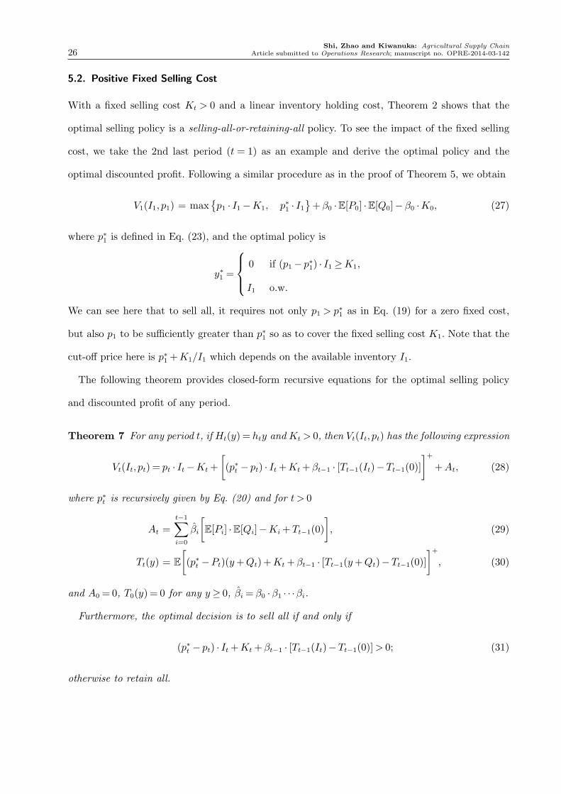
Theorem 7 For any period t, if Ht(y) = hty and Kt > 0, then Vt(It, pt) has the following expression
Vt(It, pt) = pt · It −Kt +
[(p∗t − pt) · It +Kt +βt−1 · [Tt−1(It)−Tt−1(0)]
]+
+At, (28)
where p∗t is recursively given by Eq. (20) and for t > 0
At =t−1∑i=0
βi
[E[Pi] ·E[Qi]−Ki +Tt−1(0)
], (29)
Tt(y) = E[(p∗t −Pt)(y+Qt)+Kt +βt−1 · [Tt−1(y+Qt)−Tt−1(0)]
]+
, (30)
and A0 = 0, T0(y) = 0 for any y≥ 0, βi = β0 ·β1 · · ·βi.
Furthermore, the optimal decision is to sell all if and only if
(p∗t − pt) · It +Kt +βt−1 · [Tt−1(It)−Tt−1(0)]> 0; (31)
otherwise to retain all.

Shi, Zhao and Kiwanuka: Agricultural Supply ChainArticle submitted to Operations Research; manuscript no. OPRE-2014-03-142 27
6. Numerical Study: Kenya Cooperative Coffee Exporters
In this section, we conduct a numerical study based on the real-life data of a grower organization
in Kenya, Kenya Cooperative Coffee Exporters (KCCE). Our objective is to quantify the optimal
selling policies and their potential impact on practice. We shall also illustrate the sensitivity of the
optimal policy and its performance with respect to various parameters, such as holding cost, time
horizon, and discounted rate, as well as the price process.
KCCE was founded in 2009 by small-scale grower cooperatives in Kenya to market their coffee.
KCCE conducts secondary processing, storage, marketing and distribution for its own brand of
coffee named KEN CAFE. Not only does KCCE consolidate the supply chain but also unite the
ownership and control of the coffee in one entity. With the ownership of the coffee, KCCE can
control the amount of coffee sold in each season and retain the rest to future seasons for a potentially
better price. KCCE sells weekly at Nairobi coffee auction year around (not every week, depending
on the crop seasons).
We retrieve the weekly harvest (and export) and selling price data of KCCE at the Nairobi Coffee
Exchange (auction) from 11/16/2010 to 2/22/2011. Consistent to the empirical study in §3.3, a
statistical study shows that the exports of KCCE are independent of KCCE’s selling prices, the har-
vests (in 50kg bags) follow an i.i.d. process with a marginal distribution of Normal(173.32,148.74),
and the price process of KCCE (in US$ per 50kg bag) follows an AR(1) process as
Pt−1 = 165.4+0.6886Pt + ϵt, ϵt ∼Normal(0,46.5). (32)
We set other parameters for the numerical study in the following way: we follow Sengupta and
Wang (1991) and Berg (1987) to set the inventory holding cost to be $0, $2, $4, · · · , $40 (per 50kg
bag per week). The discounted rate is obtained from the interest rate of the treasury bill issued
by the Kenya government, about 3% a year (Central Bank of Kenya, 8/2010); which leads to a
weekly discounted rate of β = 99.84%. To study the impact of the discounted rate, we also vary β
over β = 80%, 85%, 90% and 95%. The transaction costs of selling are obtained from Coffee Board
of Kenya which are bundled into a variable cost and subtracted from the price. Hence, the model
with zero fixed selling cost and linear holding cost applies here. As a benchmark, we compute the
discounted profit for the prevailing selling-all policy (“SA”) for every instance and compare it to
that of the optimal policy (the selling-all-retaining-all policy – “SARA”). All numerical studies
are conducted on the observed sample path of the actual harvest of KCCE. Finally, to study the
impact of the price process, we shall consider both i.i.d. and AR(1) price processes.

Shi, Zhao and Kiwanuka: Agricultural Supply Chain28 Article submitted to Operations Research; manuscript no. OPRE-2014-03-142
6.1. I.I.D. Price Process
In this section, we ignore the autocorrelation among prices in consecutive periods (as specified
in Eq. 32), and model the price process as a series of i.i.d. random variables but with the same
marginal distribution. In particular, according to Eq. (32), we calculate the marginal distribution of
the price to be P ∼Normal(530.8, 149.2) (in US$ per 50kg bag), which is used as the distribution
for the price in each period. Our objective is to develop insights on the optimal selling policy for
i.i.d. price processes and also to use the results as a benchmark for comparison with those of AR(1)
price process.
We compute the optimal cut-off prices for various inventory holding costs, time horizons and
discounted rates. Figures 3-4 summarize the results and reveal the following insights:
�������
�������
�������
�������
�������
�������
�������
�������
� � �� �� � � � � �� �� ��
�������
���
��� ���������� �����
������������ ������������������ �����
����� ��� ��������������
����
����
�����
p*=$795.53
p*=$731.41
p*=$688.72
Figure 3 Asymptotic Analysis of Cut-off Price
��������
��������
��������
��������
��������
��������
��������
�� ��� ��� ��� ���� ���� ���� ���� ����
������������
� ������� ������
Cut-off Price vs Holding Cost (with Selected Discount Rates)
���
���
���
���
Figure 4 Cut-off Price vs. Holding Cost
• The optimal cut-off price increases in the number of periods (weeks) left in the planning
horizon and exponentially converges to the steady-state value p∗ as the number of periods goes to
infinity, confirming our analysis in §5.1.
• The optimal cut-off price could be either above or below the average price, and it decreases in
h and increases in β.
To assess the potential impact of the SARA policy, we compare SARA and SA policies on
their Expected NPV, that is, the expected net present value of the profits over the periods from
11/16/2010 to 2/22/2011. Specifically, we randomly generate weekly prices (according to the i.i.d.
price process assumed above) for 106 replications (or sample paths). For each sample path (repli-
cation) of the prices, we apply the optimal SARA policy and the SA policy, and compute their
NPVs respectively. Finally, we take the average of the NPVs over all replications under each policy
to obtain the expected NPV.
Shi, Zhao and Kiwanuka: Agricultural Supply ChainArticle submitted to Operations Research; manuscript no. OPRE-2014-03-142 29
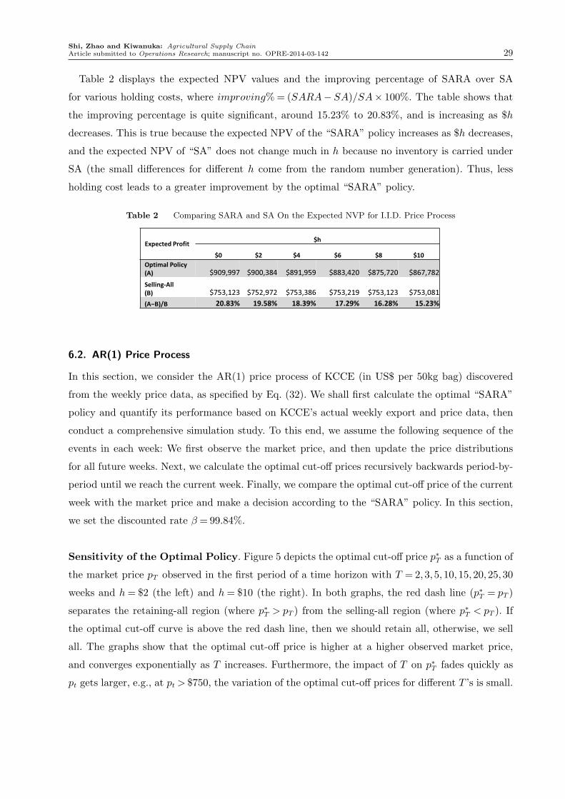
Table 2 displays the expected NPV values and the improving percentage of SARA over SA
for various holding costs, where improving%= (SARA− SA)/SA× 100%. The table shows that
the improving percentage is quite significant, around 15.23% to 20.83%, and is increasing as $h
decreases. This is true because the expected NPV of the “SARA” policy increases as $h decreases,
and the expected NPV of “SA” does not change much in h because no inventory is carried under
SA (the small differences for different h come from the random number generation). Thus, less
holding cost leads to a greater improvement by the optimal “SARA” policy.
Table 2 Comparing SARA and SA On the Expected NVP for I.I.D. Price Process
����������� ���
������ �� �� �� �� ���
��� ������ ���
���� �������� �������� ������ �������� ������� ��������
���� � !�������
�"� ������ ������� ������� ������ ������ ������
��#"�$" ������ ����� ������ ����� ������ �����
6.2. AR(1) Price Process
In this section, we consider the AR(1) price process of KCCE (in US$ per 50kg bag) discovered
from the weekly price data, as specified by Eq. (32). We shall first calculate the optimal “SARA”
policy and quantify its performance based on KCCE’s actual weekly export and price data, then
conduct a comprehensive simulation study. To this end, we assume the following sequence of the
events in each week: We first observe the market price, and then update the price distributions
for all future weeks. Next, we calculate the optimal cut-off prices recursively backwards period-by-
period until we reach the current week. Finally, we compare the optimal cut-off price of the current
week with the market price and make a decision according to the “SARA” policy. In this section,
we set the discounted rate β = 99.84%.
Sensitivity of the Optimal Policy. Figure 5 depicts the optimal cut-off price p∗T as a function of
the market price pT observed in the first period of a time horizon with T = 2,3,5,10,15,20,25,30
weeks and h= $2 (the left) and h= $10 (the right). In both graphs, the red dash line (p∗T = pT )
separates the retaining-all region (where p∗T > pT ) from the selling-all region (where p∗T < pT ). If
the optimal cut-off curve is above the red dash line, then we should retain all, otherwise, we sell
all. The graphs show that the optimal cut-off price is higher at a higher observed market price,
and converges exponentially as T increases. Furthermore, the impact of T on p∗T fades quickly as
pt gets larger, e.g., at pt > $750, the variation of the optimal cut-off prices for different T ’s is small.
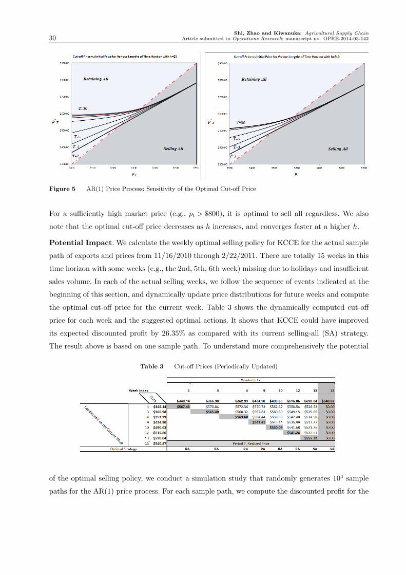
Shi, Zhao and Kiwanuka: Agricultural Supply Chain30 Article submitted to Operations Research; manuscript no. OPRE-2014-03-142
Figure 5 AR(1) Price Process: Sensitivity of the Optimal Cut-off Price
For a sufficiently high market price (e.g., pt > $800), it is optimal to sell all regardless. We also
note that the optimal cut-off price decreases as h increases, and converges faster at a higher h.
Potential Impact. We calculate the weekly optimal selling policy for KCCE for the actual sample
path of exports and prices from 11/16/2010 through 2/22/2011. There are totally 15 weeks in this
time horizon with some weeks (e.g., the 2nd, 5th, 6th week) missing due to holidays and insufficient
sales volume. In each of the actual selling weeks, we follow the sequence of events indicated at the
beginning of this section, and dynamically update price distributions for future weeks and compute
the optimal cut-off price for the current week. Table 3 shows the dynamically computed cut-off
price for each week and the suggested optimal actions. It shows that KCCE could have improved
its expected discounted profit by 26.35% as compared with its current selling-all (SA) strategy.
The result above is based on one sample path. To understand more comprehensively the potential
Table 3 Cut-off Prices (Periodically Updated)
of the optimal selling policy, we conduct a simulation study that randomly generates 103 sample
paths for the AR(1) price process. For each sample path, we compute the discounted profit for the
Shi, Zhao and Kiwanuka: Agricultural Supply ChainArticle submitted to Operations Research; manuscript no. OPRE-2014-03-142 31
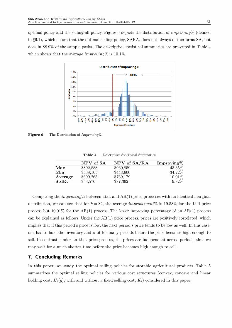
optimal policy and the selling-all policy. Figure 6 depicts the distribution of improving% (defined
in §6.1), which shows that the optimal selling policy, SARA, does not always outperforms SA, but
does in 88.9% of the sample paths. The descriptive statistical summaries are presented in Table 4
which shows that the average improving% is 10.1%.
Figure 6 The Distribution of Improving%
Table 4 Descriptive Statistical Summaries
NPV of SA NPV of SA/RA Improving%Max $892,888 $960,859 43.35%Min $538,105 $448,600 -34.22%Average $699,265 $769,179 10.01%StdEv $53,576 $87,362 9.82%
Comparing the improving% between i.i.d. and AR(1) price processes with an identical marginal
distribution, we can see that for h= $2, the average improvement% is 19.58% for the i.i.d price
process but 10.01% for the AR(1) process. The lower improving percentage of an AR(1) process
can be explained as follows: Under the AR(1) price process, prices are positively correlated, which
implies that if this period’s price is low, the next period’s price tends to be low as well. In this case,
one has to hold the inventory and wait for many periods before the price becomes high enough to
sell. In contrast, under an i.i.d. price process, the prices are independent across periods, thus we
may wait for a much shorter time before the price becomes high enough to sell.
7. Concluding Remarks
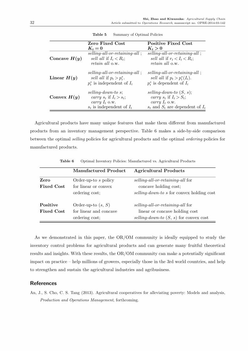
In this paper, we study the optimal selling policies for storable agricultural products. Table 5
summarizes the optimal selling policies for various cost structures (convex, concave and linear
holding cost, Ht(y), with and without a fixed selling cost, Kt) considered in this paper.
Shi, Zhao and Kiwanuka: Agricultural Supply Chain
32 Article submitted to Operations Research; manuscript no. OPRE-2014-03-142
Table 5 Summary of Optimal Policies
Zero Fixed Cost Positive Fixed CostKt = 0 Kt > 0selling-all-or-retaining-all ; selling-all-or-retaining-all ;
Concave H(y) sell all if It <Rt; sell all if rt < It <Rt;retain all o.w. retain all o.w.
selling-all-or-retaining-all ; selling-all-or-retaining-all ;Linear H(y) sell all if pt > p∗t . sell all if pt > p∗t (It).
p∗t is independent of It p∗t is dependent of It
selling-down-to s; selling-down-to (S, s);Convex H(y) carry st if It > st; carry st if It >St;
carry It o.w. carry It o.w.st is independent of It st and St are dependent of It
Agricultural products have many unique features that make them different from manufactured
products from an inventory management perspective. Table 6 makes a side-by-side comparison
between the optimal selling policies for agricultural products and the optimal ordering policies for
manufactured products.
Table 6 Optimal Inventory Policies: Manufactured vs. Agricultural Products
Manufactured Product Agricultural Products
Zero Order-up-to s policy selling-all-or-retaining-all for
Fixed Cost for linear or convex concave holding cost;
ordering cost; selling-down-to s for convex holding cost
Positive Order-up-to (s, S) selling-all-or-retaining-all for
Fixed Cost for linear and concave linear or concave holding cost
ordering cost; selling-down-to (S, s) for convex cost
As we demonstrated in this paper, the OR/OM community is ideally equipped to study the
inventory control problems for agricultural products and can generate many fruitful theoretical
results and insights. With these results, the OR/OM community can make a potentially significant
impact on practice – help millions of growers, especially those in the 3rd world countries, and help
to strengthen and sustain the agricultural industries and agribusiness.
References
An, J., S. Cho, C. S. Tang (2013). Agricultural cooperatives for alleviating poverty: Models and analysis,
Production and Operations Management, forthcoming.
Shi, Zhao and Kiwanuka: Agricultural Supply Chain
Article submitted to Operations Research; manuscript no. OPRE-2014-03-142 33
Akiyama, T., P. N. Varangis, (1990). The impact of the International Coffee Agreement on producing coun-
tries, World Bank Economic Review, 4(1): 157-173.
Alaouze, C. M., N. H. Sturgess, A.S. Watson, (1978). Australian wheat storage: A dynamic programming
approach, Australian Journal of Agricultural Economics, 22(3).
Berg, E. (1987). A sequential decision model to determine optimal farm-level grain marketing policies,
European Review of Agricultural Economics, 14: 091-116.
Bertsekas, D. P. (1976). Dynamic programming and stochastic control. Mathematics in Science and Engi-
neering, Vol. 123.
Bhaskaran, S., K. Ramachandran, J. Semple, (2010). A dynamic inventory model with the right of refusal.
Management Science, 56(12), 2265-2281.
Blakeslee, L. (1997). Optimal sequential grain marketing decisions under risk aversion and price uncertainty,
American Journal of Agricultural Economics, 79(4): 1140-1152.
Boyabatli, O., L. B. Toktay, (2004). Operational hedging: A review with discussion. Tech. rep.
Chen, X., D. Simchi-Levi, (2004). Coordinating inventory control and pricing strategies with random demand
and fixed ordering cost: The finite horizon case. Operations Research, 52(6), 887-896.
Daviron, B., S. Ponte (2006). The Coffee Paradox: Global Markets, Commodity Trade and the Elusive Promise
of Development. Zed Books Ltd, London, UK.
Dugundji, J., A. Granas (2010). Fixed Point Theory. Springer, New York.
Fackler, P. L., M. J. Livingston (2002). Optimal storage by crop producers, American Journal of Agriculture
Economics, 84(3): 645-659.
Federgruen, A., A. Heching, (1999). Combined pricing and inventory control under uncertainty. Operations
research, 47(3), 454-475.
Gustafson, R. L. (1958). Carryover levels for grain: A method for determining amounts that are optimal
under specified conditions, USDA Tech. Bull No. 1178, Washington, D.C.
Huchzermeier, A., M. A. Cohen, (1996). Valuing operational flexibility under exchange rate risk. Operations
research, 44(1), 100-113.
Kawanuka, R. K., Y. Zhao (2009). From farm to cup: The coffee supply chain in Kenya, Case Study – Rutgers
Business School-Newark and New Brunswick.
Kazaz, B., S. Webster, (2011). The impact of yield-dependent trading costs on pricing and production
planning under supply uncertainty. Manufacturing & Service Operations Management, 13(3), 404-417.
Knapp, K. C. (1982). Optimal grain carryovers in open economies: A graphical analysis, American Journal
of Agricultural Economics, 64(2): 197.
Lai, J. Y., R. J. Myers, S. D. Hanson (2003). Optimal on-farm grain storage by risk-averse farmers, Journal
of Agricultural and Resource Economics, 28(3): 558-579.

Shi, Zhao and Kiwanuka: Agricultural Supply Chain
34 Article submitted to Operations Research; manuscript no. OPRE-2014-03-142
Nyangito, H. O. (2002). Policy and legal framework for the coffee subsector and the impact of liberalization in
Kenya, KIPPRA Policy Paper No. 2., Kenya Institute of Public Policy Research and Analysis, Nairobi.
Osorio, N. (2002). Technological developments on coffee: Constraints encountered by producing countries.
International Coffee Organisation.
Oxfam International Commodity Research (2001). The coffee market: a background study,
http://www.maketradefair.com/en/assets/english/BackgroundStudyCoffeeMarket.pdf.
Pindyck, R. S., D. L. Rubinfeld (1998). Econometric Models and Economic Forecasts, 4th Ed. Irwin/McGraw-
Hill International Editions.
Ponte, S. (2002). The latte revolution? regulation, markets and consumption in the global coffee chain, World
Development, 30: 1099-1122.
Porteus, E. L. (2002). Foundations of Stochastic Inventory Theory. Stanford University Press. CA
Prabhu, N. U. (1998). Stochastic Storage Processes: Queues, Insurance Risk, Dams, and Data Communica-
tion, 2nd edition. Springer, New York.
Sengupta, J. K., E. C. Wang, (1991). Market structure implications of instability in the world coffee market,
Economic Modeling, 8(1): 102-115.
Sheskin, D. (2000). Handbook of parametric and nonparametric statistical procedures; Second Ed. Chapman
and Hall/CRC, New York.
Simchi-Levi, D., J. Bramel, X. Chen, (2005). The Logic of Logistics: Theory, Algorithms, and Applications
for Logistics and Supply Chain management. Springer.
Simchi-Levi, D., Y. Zhao, (2011). Performance evaluation of stochastic multi-echelon inventory systems: A
survey. Advances in Operations Research, Volume 2012.
Tomlin, B. (2006). On the value of mitigation and contingency strategies for managing supply chain disruption
risks. Management Science, 52(5), 639-657.
Tomlin, B., Y. Wang (2005). On the value of mix flexibility and dual sourcing in unreliable Newsvendor
networks. Manufacturing & Service Operations Management, 7(1), 37-57.
Topkis, D. M. (1998), Supermodularity and Complementarity, Princeton University Press.
Tronstad, R., C. R. Taylor (1991). Dynamically optimal after-tax grain storage, cash grain sale, and hedging
strategies, American Journal of Agricultural Economics, 73(1): 75-88.
Ugarte, M. D., A. F. Militino, A. T. Arnholt (2008). Probability and Statistics with R. Taylor and Francis
Group, LLC.
Van Mieghem, J. A. (1999). Coordinating investment, production, and subcontracting. Management Science,
45(7), 954-971.
Van Mieghem, J. A. (2003). Capacity management,investment, and hedging:Review and recent developments,
Manufacturing & Service Operations Management, 5(4), 269-302.
Shi, Zhao and Kiwanuka: Agricultural Supply Chain
Article submitted to Operations Research; manuscript no. OPRE-2014-03-142 35
Van Mieghem, J. A. (2007). Risk mitigation in Newsvendor networks: resource diversification, flexibility,
sharing, and hedging. Management Science, 53(8), 1269-1288.
Wang, Y., Y. Gerchak, (1996). Periodic review production models with variable capacity, random yield, and
uncertain demand. Management science, 42(1), 130-137.
Wang, Y., W. Gilland, B. Tomlin, (2010). Mitigating supply risk: Dual sourcing or process improvement?.
Manufacturing & Service Operations Management, 12(3), 489-510.
Wright, B. (2001). Storage and price stabilization. Chapter 14 in Handbook of agricultural economics (Ed.)
Bruce L. Gardner and Gordon C. Rausser, 817-861. Elsevier.
Yano, C. A., H. L. Lee, (1995). Lot sizing with random yields: A review. Operations Research, 43(2), 311-334.
Zipkin, P. (2000). Foundations of Inventory Management. McGraw Hill, Boston.
Shi, Zhao and Kiwanuka: Agricultural Supply Chain
36 Article submitted to Operations Research; manuscript no. OPRE-2014-03-142
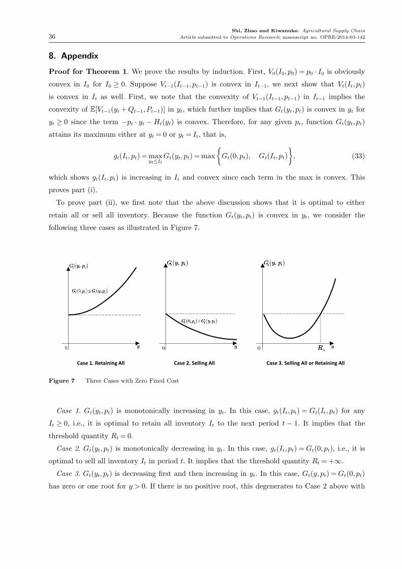
8. Appendix
Proof for Theorem 1. We prove the results by induction. First, V0(I0, p0) = p0 · I0 is obviously
convex in I0 for I0 ≥ 0. Suppose Vt−1(It−1, pt−1) is convex in It−1, we next show that Vt(It, pt)
is convex in It as well. First, we note that the convexity of Vt−1(It−1, pt−1) in It−1 implies the
convexity of E[Vt−1(yt +Qt−1, Pt−1)] in yt, which further implies that Gt(yt, pt) is convex in yt for
yt ≥ 0 since the term −pt · yt −Ht(yt) is convex. Therefore, for any given pt, function Gt(yt, pt)
attains its maximum either at yt = 0 or yt = It, that is,
gt(It, pt) =maxyt≤It
Gt(yt, pt) =max
{Gt(0, pt), Gt(It, pt)
}, (33)
which shows gt(It, pt) is increasing in It and convex since each term in the max is convex. This
proves part (i).
To prove part (ii), we first note that the above discussion shows that it is optimal to either
retain all or sell all inventory. Because the function Gt(yt, pt) is convex in yt, we consider the
following three cases as illustrated in Figure 7.
��������������� �� ��������������� �� ��������������� ������������� ��
Figure 7 Three Cases with Zero Fixed Cost
Case 1. Gt(yt, pt) is monotonically increasing in yt. In this case, gt(It, pt) = Gt(It, pt) for any
It ≥ 0, i.e., it is optimal to retain all inventory It to the next period t − 1. It implies that the
threshold quantity Rt = 0.
Case 2. Gt(yt, pt) is monotonically decreasing in yt. In this case, gt(It, pt) =Gt(0, pt), i.e., it is
optimal to sell all inventory It in period t. It implies that the threshold quantity Rt =+∞.
Case 3. Gt(yt, pt) is decreasing first and then increasing in yt. In this case, Gt(y, pt) =Gt(0, pt)
has zero or one root for y > 0. If there is no positive root, this degenerates to Case 2 above with

Shi, Zhao and Kiwanuka: Agricultural Supply Chain
Article submitted to Operations Research; manuscript no. OPRE-2014-03-142 37
Rt =+∞ where it is optimal to sell all inventory. For the other case with a unique positive root
Rt > 0, we have Gt(y, pt)<Gt(0, pt) =Gt(Rt, pt) for 0< y <Rt which implies it is optimal to sell
all inventory; Gt(y, pt) is increasing and Gt(y, pt)>Gt(0, pt) =Gt(Rt, pt) for y > Rt, which shows
that it is optimal to retain all inventory.
The proof for part (ii) is completed by concluding all the above cases. �
Proof for Proposition 1. To prove part (i), we apply induction. First, for the last period,
∂2G1(y1, p1)/(∂y1∂p1) = β0 ·E[∂2V0(y1 +Q0,A0 · f(p1)+B0)/(∂y∂p) · A0f′0(p1)]− 1
= β0 ·E[A0f′0(p1)]− 1≤ 0, (34)
where the first equality holds by ∂2V0(I0, p0)/∂I0∂p0 = 1 and the inequality holds by assumption
0≤ f ′0(p)E[A0]≤ 1. Furthermore, by Eq. (33), one has
g1(I1, p1) =
{G1(0, p1), if I1 <R1;
G1(I1, p1), o.w.(35)
Hence, ∂2g1(I1, p1)/(∂I1∂p1)≤ 0, which further implies, ∂2V1(I1, p1)/(∂I1∂p1)≤ 1 by Eq. (1).
Next in induction, we assume that Eq. (8) holds for any period from period 0 through period
t− 1. We shall prove that it still holds for period t. To this end, taking partial derivatives of Eq.
(3) with respect to yt and pt yields,
∂2Gt(yt, pt)/(∂yt∂pt) = βt−1 ·E[∂2Vt−1(yt +Qt−1,At−1 · f(pt)+Bt−1)/(∂y∂p) · At−1 · f ′t−1(pt)]− 1,
≤ βt−1 ·E[At−1 · f ′t−1(pt)]− 1≤ 0.
By Eq. (33), one has
gt(It, pt) =
{Gt(0, pt), if It <Rt;
Gt(It, pt), o.w.(36)
Hence, ∂2gt(It, pt)/(∂It∂pt) ≤ 0, which further implies, ∂2Vt(It, pt)/(∂It∂pt) ≤ 1 by Eq. (1). The
proof for part (i) is now completed.
To prove part (ii), we first note that for the trivial cases of Rt(pt) = 0 or Rt(pt) =+∞, it holds
obviously. In what follows, we focus on the case with a finite positive value, i.e., Case 3 in Figure 7.
To this end, consider two distinct prices p < p′, and denote their corresponding threshold values as
R≡R(p) and R′ ≡R′(p′), we shall prove R<R′. First, by Theorem 1, we have Gt(0, p′) =Gt(R
′, p′)
and Gt(0, p) =Gt(R,p). Then, taking the difference on both sides yields
Gt(0, p′)−Gt(0, p) = Gt(R
′, p′)−Gt(R,p);
Shi, Zhao and Kiwanuka: Agricultural Supply Chain
38 Article submitted to Operations Research; manuscript no. OPRE-2014-03-142
= [Gt(R′, p′)−Gt(R,p′)]+ [Gt(R,p′)−Gt(R,p)].
Rearranging the above, we further have
Gt(R′, p′)−Gt(R,p′) = [Gt(0, p
′)−Gt(0, p)]− [Gt(R,p′)−Gt(R,p)]≥ 0,
where the inequality holds by ∂2Gt(y, p)/(∂y ∂p) ≥ 0 as given in part (i). Note that Gt(R,p) is
increasing in the neighborhood of R (cf. Case 3 in Figure 7), hence, we must have R′ ≥R, which
completes the proof for part (ii). �
Proof for Proposition 2. Under Assumption 2, we first rewrite the dynamic programming equa-
tion as
Vt(It, pt) = max0≤yt≤It
{pt · (It − yt)−Ht(yt)+βt−1 · vt−1(yt, pt)
}, (37)
where vt−1(yt, pt)≡E[Vt−1(yt+Qt−1, At−1 ·ft−1(pt)+Bt−1)
]. We shall prove the result by induction.
For the last period, V0(I0, p0) is increasing and linear in p0. Assuming that the result holding for
period 0 through t− 1, we shall prove it still holds for period t. The increasing property in pt can
been justified as follows: ft−1(p) increases in p, then vt−1(yt, pt) increases in p as well; ultimately,
Eq. (37) shows Vt−1(yt, pt) increases in pt. We next prove its concavity by definition. For p′ < p′′,
the concavity of ft−1(·) shows that for any λ∈ [0,1],
ft−1(λp′ +(1−λ)p′′)≥ λft−1(p
′)+ (1−λ)ft−1(p′′). (38)
Therefore, for any given yt, we have
vt−1(yt, λp′ +(1−λ)p′′)
= E[Vt−1(yt +Qt−1,At−1 · ft−1(λp′ +(1−λ)p′′)+Bt−1)]
≥ E[Vt−1(yt +Qt−1,At−1[λft−1(p′)+ (1−λ)ft−1(p
′′)]+Bt−1)]
= E[Vt−1
(yt +Qt−1, λ[At−1ft−1(p
′)+Bt−1] + (1−λ)[At−1ft−1(p′′)+Bt−1]
)]≥ λE[Vt−1(yt +Qt−1,At−1ft−1(p
′)+Bt−1)]+ (1−λ)E[Vt−1(yt +Qt−1,At−1ft−1(p′′)+Bt−1)]
= λvt−1(yt, p′)+ (1−λ)vt−1(yt, p
′′),
where the first inequality holds by Eq. (38) and the assumption that At−1 is a nonnegative random
variable. The above proves that the vt−1 is concave in pt. Finally, Eq. (37) shows that Vt−1 is
concave in pt, which completes the proof. �

Shi, Zhao and Kiwanuka: Agricultural Supply Chain
Article submitted to Operations Research; manuscript no. OPRE-2014-03-142 39
Proof for Theorem 2. We prove the result by induction. First, V0(I0, p0) = p0 · I0 − δ(I0) ·K0
is obviously convex in I0 for I0 ≥ 0. Suppose Vt−1(It−1, pt−1) is convex in It−1, we now show that
Vt(It, pt) is convex in It as well. To this end, we note that the convexity of Vt−1(It−1, pt−1) in
It−1 implies the convexity of E[Vt−1(yt +Qt−1, Pt−1)] in yt, which further implies that Gt(yt, pt) is
convex in yt for yt ≥ 0 since the term −pt ·yt−Ht(yt) is convex. Therefor, for any given pt, function
Gt(yt, pt) attains its maximum at either yt = 0 or yt = It, that is,
gt(It, pt) =maxyt≤It
Gt(yt, pt) =max
{Gt(0, pt)−Kt, Gt(It, pt)
},
which shows gt(It, pt) is increasing in It and convex since each term in the max is convex. This
proves part (i).
We next prove part (ii) by considering the following three cases as illustrated in Figure 8.
��������������� �� ��������������� �� ��������������� ������������� ��
Figure 8 Three Cases with Fixed Cost
Case 1. Gt(yt, pt) is monotonically increasing in yt. In this case, gt(It, pt) = Gt(It, pt) for any
It ≥ 0, i.e., it is always optimal to retain all inventory to the next period t− 1. This represents the
degenerated case where rt =Rt = 0.
Case 2. Gt(yt, pt) is monotonically decreasing in yt. In this case, gt(It, pt) = Gt(0, pt) −Kt if
It ≤ rt, i.e., it is optimal to sell all inventory; otherwise, gt(It, pt) =Gt(It, pt), i.e., it is optimal to
retain all inventory. This represents the degenerated case where Rt =+∞.
Case 3. Gt(yt, pt) is decreasing first and then increasing in yt. In this case, Gt(y, pt) =Gt(0, pt)−
Kt has zero, one or two roots for y > 0. If there is none or just one positive root, Gt(y, pt) ≥
Gt(0, pt)−Kt, then it is degenerated to Case 1 above where it is optimal to retain all inventory.
If there are two distinct positive roots 0< rt <Rt, then Gt(y, pt)<Gt(0, pt)−Kt for rt < y <Rt,
Shi, Zhao and Kiwanuka: Agricultural Supply Chain
40 Article submitted to Operations Research; manuscript no. OPRE-2014-03-142
which implies it is optimal to sell all inventory; Gt(y, pt)>Gt(0, pt)−Kt for y < rt or y >Rt, which
shows that it is optimal to retain all inventory.
The proof of part (ii) is completed by summarizing all the three cases above. �
Proof for Proposition 3. In view of Theorem 2, Eq. (12) implies rt =Rt = 0, which means that
it is optimal to retain all inventory for any It. This proves part (i). Part (ii) is readily seen from
Eqs. (10)-(11).
To prove (iii), we first prove the following inequalities via induction:
∂2Vt(I, p)
∂I · ∂p≤ 1;
∂2Gt(y, p)
∂y · ∂p≤ 0; (39)
First, for period t= 1, we have
∂2G1(y1, p1)/(∂y1∂p1) = β0 ·E[∂2V0(y1 +Q0,A0 · f(p1)+B0)/(∂y∂p) · A0f′0(p1)]− 1
= β0 ·E[A0f′0(p1)]− 1≤ 0,
where the first equality holds because ∂2V0(I0, p0)/∂I0∂p0 = 1 and the inequality holds because
0≤ f ′0(p)E[A0]≤ 1 by Assumption 2. Furthermore, by Theorem 2, one has
g1(I1, p1) =
{G1(0, p1)−K1, if I1 ∈ (r1, R1);
G1(I1, p1), o.w.(40)
Hence, ∂2g1(I1, p1)/(∂I1∂p1)≤ 0, which further implies, ∂2V1(I1, p1)/(∂I1∂p1)≤ 1 by Eq. (1).
Next in induction, we assume that Eq. (39) holds for any period from period 0 through period
t− 1. We shall prove that still holds for period t. To this end, taking partial derivatives of Eq. (3)
with respect to yt and pt yields,
∂2Gt(yt, pt)/(∂yt∂pt) = βt−1 ·E[∂2Vt−1(yt +Qt−1,At−1 · f(pt)+Bt−1)/(∂y∂p) · At−1 · f ′t−1(pt)]− 1,
≤ βt−1 ·E[At−1 · f ′t−1(pt)]− 1≤ 0.
By Theorem 2, one has
gt(It, pt) =
{Gt(0, pt)−Kt, if It ∈ (rt, Rt);
Gt(It, pt), o.w.(41)
Hence, ∂2gt(It, pt)/(∂It ·x∂pt)≤ 0, which further implies, ∂2Vt(It, pt)/(∂It∂pt)≤ 1 by Eq. (1). The
proof for Eq. (39) is now completed.
To prove part (iii), we first note that for the trivial cases of Rt(pt) = 0 or Rt(pt) =+∞, the result
holds obviously. In what follows, we shall focus on the representative case with finite positive values,
Shi, Zhao and Kiwanuka: Agricultural Supply Chain
Article submitted to Operations Research; manuscript no. OPRE-2014-03-142 41
i.e., Case 3 in Figure 8. To this end, we consider two prices p < p′, and denote their corresponding
threshold values r≡ r(p) and r′ ≡ r′(p′), R≡R(p) and R′ ≡R′(p′). Hence, it is sufficient to prove
r > r′ and R<R′.
Proof for R<R′: First, by Eq. (11), we have Gt(0, p′) − Kt = Gt(R
′, p′) and Gt(0, p) − Kt =
Gt(R,p). Then, taking the difference on both sides yields
Gt(0, p′)−Gt(0, p) = Gt(R
′, p′)−Gt(R,p);
= [Gt(R′, p′)−Gt(R,p′)]+ [Gt(R,p′)−Gt(R,p)].
Hence, we have
Gt(R′, p′)−Gt(R,p′) = [Gt(0, p
′)−Gt(0, p)]− [Gt(R,p′)−Gt(R,p)]≥ 0,
where the inequality holds by ∂2Gt(y, p)/(∂y · ∂p)≥ 0 as given by Eq. (39). Note that Gt(R,p) is
increasing in the neighborhood of R (cf. Case 3 in Figure 8). Hence, we must have R′ ≥R.
Proof for r > r′: First, by Eq. (10), we have Gt(0, p′)−Kt =Gt(r
′, p′) and Gt(0, p)−Kt =Gt(r, p).
In a similar vein as above, we have
Gt(r′, p′)−Gt(r, p
′) = [Gt(0, p′)−Gt(0, p)]− [Gt(r, p
′)−Gt(r, p)]≥ 0,
where the inequality holds by ∂2Gt(y, p)/(∂y · ∂p)≥ 0 as given by Eq. (39). Note that Gt(r, p) is
decreasing in the neighborhood of r (cf. Case 3 in Figure 8). Hence, we must have r′ ≤ r.
These analyzes complete the proof for part (iii). �
Proof for Theorem 3. We prove the results via induction. First, V0(I0, p0) = p0 · I0 is obviously
concave in I0 for I0 ≥ 0. Therefore,
G1(y1, p1) = −p1 · y1 −H1(y1)+β0 ·E[(y1 +Q0)P0|p1];
= (β0 ·E[P0|p1]− p1) · y1 −H1(y1)+β0 ·E[Q0] ·E[P0|p1]
is concave given that the first term on the right side above is linear and H1(·) is convex by
assumption. Hence, there exists s1 ≥ 0 such that
g1(I1, p1) = max0≤yt≤It
{G(y1, p1)
}=
{G1(s1, p1), if I1 ≥ s1;
G1(I1, p1), o.w.
which shows that g1(I1, p1) is concave as well in I1.Therefore, V1(I1, p1) = I1 · p1 + g1(I1, p1) is
concave in I1.
Shi, Zhao and Kiwanuka: Agricultural Supply Chain
42 Article submitted to Operations Research; manuscript no. OPRE-2014-03-142
Now suppose for any period t, Vt−1(It−1, pt−1) is concave in It−1. Therefore, E[Vt−1(It−1, Pt−1)|pt]
is concave in It−1, and hence it is also concave in yt given that It−1 = yt+Qt−1 is linear. Then, we
have Gt(yt, pt) is concave in yt since −pt · yt −Ht(yt) is concave. This completes the proof for part
(i).
Note that gt(It, pt) is increasing in It. Therefore, V (It, pt) is increasing in It as well. This proves
part (ii).
In view of part (i), there exists a unique maximum st = argmaxyt≥0{Gt(yt, pt)} and the optimal
carry-over inventory is given by Eq. (13), which completes the proof for part (iii). �
Proof for Proposition 4. To prove part (i), we use induction. First, for period t= 1, we have
∂2G1(y1, p1)/(∂y1∂p1) = β0 ·E[∂2V0(y1 +Q0,A0 · f(p1)+B0)/(∂y∂p) · A0f′0(p1)]− 1
= β0 ·E[A0f′0(p1)]− 1≤ 0
where the first equality holds by ∂2V0(I0, p0)/∂I0 · ∂p0 = 1 and the inequality holds by 0 ≤
f ′0(p)E[A0]≤ 1 according to Assumption 2. By Theorem 3, one has
g1(I1, p1) =
{G1(s1, p1), if I1 > s1;
G1(I1, p1), o.w.
Hence, ∂2g1(I1, p1)/(∂I1 · ∂p1)≤ 0, which further implies, ∂2V1(I1, p1)/(∂I1 · ∂p1)≤ 1 by Eq. (1).
Next in induction, we assume that Eq. (15) holds for any period from period 0 through period
t− 1. We shall prove that still holds for period t. To this end, taking partial derivatives of Eq. (3)
with respect to yt and pt yields,
∂2Gt(yt, pt)/(∂yt · ∂pt) = βt−1 ·E[∂2Vt−1(yt +Qt−1,At−1 · f(pt)+Bt−1)/(∂y∂p) · At−1 · f ′t−1(pt)]− 1,
≤ βt−1 ·E[At−1 · f ′t−1(pt)]− 1≤ 0.
By Eq. (33), one has
gt(It, pt) =
{Gt(st, pt), if It > st;
Gt(It, pt), o.w.(42)
Hence, ∂2gt(It, pt)/(∂It · ∂pt)≤ 0, which further implies, ∂2Vt(It, pt)/(∂It · ∂pt)≤ 1 by Eq. (1). The
proof for part (i) is now completed.
Part (ii) readily follows from Theorem 8 (Topkis’s Theorem) given∂2Gt(y, p)
∂y · ∂p≤ 0 from part (i).
�
Shi, Zhao and Kiwanuka: Agricultural Supply Chain
Article submitted to Operations Research; manuscript no. OPRE-2014-03-142 43
Proof for Theorem 4. We prove the results via induction. First, V0(I0, p0) = p0 ·I0−K0 is clearly
concave in view of its linearity in I0 for I0 ≥ 0. Therefore,
G1(y1, p1) = −p1 · y1 −H1(y1)+β0 ·E[(y1 +Q0)P0|p1],
is concave. By Lemma 3, the function g1(I1, p1) is K1-concave in I0.
Now suppose Vt−1(It−1, pt−1) is Kt−1-concave in It−1. Then, by Lemma 3, E[Vt−1(It−1, Pt−1)|pt]is Kt−1-concave in It−1, and hence it is also Kt−1-concave in yt given that It−1 = yt+Qt−1 is linear.
Then, we have Gt(yt, pt) is βt−1Kt−1-concave in yt since −pt · yt −Ht(yt) is 0-concave. By Lemma
3 again, gt(It, pt) is Kt-concave given βt−1Kt−1 ≤Kt. This completes the proof for part (i).
To prove part (ii), we note that gt(It, pt) is increasing and Kt-concave in It. Therefore, V (It, pt)
is increasing and Kt-concave in It as well.
Finally, by Lemma 3, there exists a unique global maximum st = argmaxyt≥0{Gt(yt, pt)} and St
given by Eq. (17), and the optimal carry-over inventory is given by Eq. (16). �
Proof for Theorem 5. For period t with the observed price pt, we prove the result via induction.
First, in period 0, it is optimal to sell all inventory which implies p∗0 = 0. Next, we consider period
1 and the expected discounted profit is given by
V1(I1, p1) = p1 · I1 + max0≤y1≤I1
{− (p1 +h1) · y1 +β0E[P0 · (y1 +Q0) |p1]
},
= p1 · I1 + max0≤y1≤I1
{− (p1 +h1 −β0E[P0 |p1]) · y1 +β0E[P0 |p1]E[Q0]
}.
The second equality holds because the price and harvest are independent according to Assumption
1. Clearly, consistent to Theorems 1 and 3, the optimal policy is a selling-all-or-retaining-all policy
which depends on the cut-off price defined as
p∗1 = β0E[P0|p1]−h1 = β0E[max{P0, p∗0}|p1]−h1,
where p∗1 = p∗1(p1). Namely, it is optimal to sell all I1 if and only if p1 ≥ p∗1, retain all otherwise.
The optimal discounted profit V1(I1, P1) can be expressed as follows:
V1(I1, p1) = max{p1, β0E[P0|p1]−h1}I1 +β0E[P0|p1]E[Q0]
= max{p1, p∗1} · I1 +(p∗1 +h1)E[Q0]. (43)
Now consider period t= 2. With the aid of Eq. (43), the total expected profit is given by
V2(I2, p2) = p2 I2 + max0≤y2≤I2
{− (p2 +h2) · y2 + β1E
[max{P1, p
∗1(P1)}|p2
](y2 +E[Q1])

Shi, Zhao and Kiwanuka: Agricultural Supply Chain
44 Article submitted to Operations Research; manuscript no. OPRE-2014-03-142
+ β1(E[p∗1(P1)|p2] +h1)E[Q0]
}.
It is straightforward to see from the above equation that the cut-off price is given as
p∗2 = β1E[max{P1, p∗1(P1)}|p2]−h2,
where the expectation is taken with respect to P1 conditioning on p2. V2(I2, p2) can be further
written as,
V2(I2, p2) = max{p2, p∗2} · I2 +(p∗2 +h2)E[Q1] +β1(E[p∗1(P1)|p2] +h1)E[Q0].
In general, we consider any period t > 0. Suppose for any pt, there exists a cut-off price p∗t = p∗t (pt)
given recursively by Eq. (20) from period t through the last period, so that it is optimal to sell all
if pt ≥ p∗t , and retain all otherwise. We also assume Vt(It, pt) has the explicit expression given by
Eq. (21). Now for period t+1, we have
Vt+1(It+1, pt+1) = pt+1 It+1 + max0≤yt+1≤It+1
{− (pt+1 +ht+1) · yt+1 +βtE[V (yt+1,Pt)|pt+1]
}.
Next, plugging Eq. (21) into the above yields
Vt+1(It+1, pt+1) = pt+1 It+1 + max0≤yt+1≤It+1
{− (pt+1 − p∗t+1) · yt+1 +(p∗t+1 +ht+1)E[Qt]
+ βt
t∑s=1
βt,s
(E[E[p∗s|Pt]
∣∣∣∣pt+1
]+hs
)E[Qs−1]
}.
where
p∗t+1 = βtE[max{Pt, p∗t}]−ht+1,∀t≤ T − 1.
Note that βt · βt,s = βt+1,s, and E[E[p∗s|Pt]|pt+1
]=E[p∗s|pt+1] by the property of conditional expec-
tation. One can further simplify Vt+1(It+1, pt+1) as follows,
Vt+1(It+1, pt+1) = pt+1 It+1 + max0≤yt+1≤It+1
{− (pt+1 − p∗t+1)yt+1 +
t+1∑s=1
βt+1,s
(E[p∗s|pt+1] +hs
)E[Qs−1]
}
= max{pt+1, p∗t+1} · It+1 +
t+1∑s=1
βt+1,s
(E[p∗s|pt+1] +hs
)E[Qs−1].
Finally, the proof is complete via induction. �
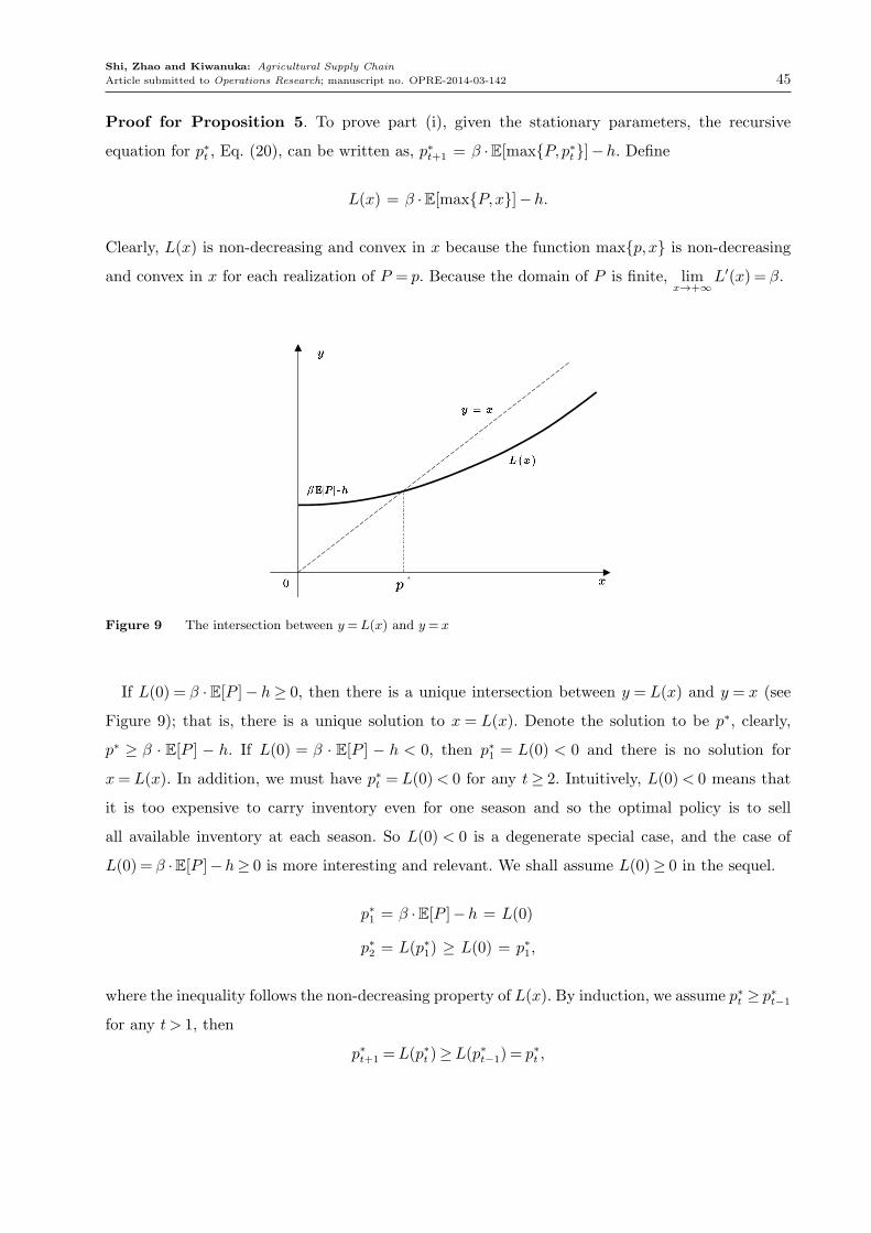
Shi, Zhao and Kiwanuka: Agricultural Supply Chain
Article submitted to Operations Research; manuscript no. OPRE-2014-03-142 45
Proof for Proposition 5. To prove part (i), given the stationary parameters, the recursive
equation for p∗t , Eq. (20), can be written as, p∗t+1 = β ·E[max{P,p∗t}]−h. Define
L(x) = β ·E[max{P,x}]−h.
Clearly, L(x) is non-decreasing and convex in x because the function max{p,x} is non-decreasing
and convex in x for each realization of P = p. Because the domain of P is finite, limx→+∞
L′(x) = β.
Figure 9 The intersection between y=L(x) and y= x
If L(0) = β ·E[P ]− h≥ 0, then there is a unique intersection between y = L(x) and y = x (see
Figure 9); that is, there is a unique solution to x = L(x). Denote the solution to be p∗, clearly,
p∗ ≥ β · E[P ] − h. If L(0) = β · E[P ] − h < 0, then p∗1 = L(0) < 0 and there is no solution for
x= L(x). In addition, we must have p∗t = L(0)< 0 for any t≥ 2. Intuitively, L(0)< 0 means that
it is too expensive to carry inventory even for one season and so the optimal policy is to sell
all available inventory at each season. So L(0) < 0 is a degenerate special case, and the case of
L(0) = β ·E[P ]−h≥ 0 is more interesting and relevant. We shall assume L(0)≥ 0 in the sequel.
p∗1 = β ·E[P ]−h = L(0)
p∗2 = L(p∗1) ≥ L(0) = p∗1,
where the inequality follows the non-decreasing property of L(x). By induction, we assume p∗t ≥ p∗t−1
for any t > 1, then
p∗t+1 =L(p∗t )≥L(p∗t−1) = p∗t ,
Shi, Zhao and Kiwanuka: Agricultural Supply Chain
46 Article submitted to Operations Research; manuscript no. OPRE-2014-03-142
which implies that as t increases, p∗t is increasing. Consequently, it is easy to show,
p∗t+1 − p∗t = β ·E[max{P,p∗t}−max{P,p∗t−1}
]≤ β · (p∗t − p∗t−1). (44)
Thus y = L(x) is a Banach contraction mapping because β < 1 (Dugundji and Granas 2010, pg
9). By Banach Fixed Point theorem, as t → +∞, p∗t increases and converges to p∗, where p∗ is
determined by p∗ =L(p∗) = β ·E[max{P,p∗}]−h, as given by Eq. (24). This completes the proof
for part (i)
To derive the steady-state limit of the optimal discounted profit in an infinite time horizon, by
Eq. (21), we know that for t≥ 0,
Vt+1(I, p) = max{p, p∗t+1}I +(p∗t+1 +h)E[Q] +β · (p∗t +h)E[Q] + . . .+βt(p∗1 +h)E[Q].
Define,
Ut+1(I, p) = max{p, p∗}I +(p∗ +h)E(Q)+β · (p∗ +h)E[Q] + . . .+βt(p∗ +h)E[Q]
= max{p, p∗}I +(p∗ +h)E(Q)1−βt+1
1−β.
Their difference can be written as follows,
∆t+1 = Ut+1(I, p)−Vt+1(I, p)
= (max{p, p∗}−max{p, p∗t+1})I +E[Q][(p∗ − p∗t+1)+β · (p∗ − p∗t )+ . . .+βt(p∗ − p∗1)].
By Eq. (44),
p∗ − p∗t+1 = p∗ − p∗t+2 + p∗t+2 − p∗t+1
= p∗ − p∗t+n + p∗t+n − p∗t+n−1 + . . .+ p∗t+2 − p∗t+1, for n> 1
≤ p∗ − p∗t+n +(p∗t+2 − p∗t+1)(1−βn−1)
1−β, for n> 1.
Let n→∞ and note that p∗t+n → p∗, we arrive at
p∗ − p∗t+1 ≤ limn→∞
[p∗ − p∗t+n +
(p∗t+2 − p∗t+1)(1−βn−1)
1−β
]=
p∗t+2 − p∗t+1
1−β.
Thus,
∆t+1 ≤(max{p, p∗}−max{p, p∗t+1}
)· I +E[Q]
[p∗t+2 − p∗t+1
1−β+β
p∗t+1 − p∗t1−β
+ . . .+βt p∗2 − p∗11−β
]
Shi, Zhao and Kiwanuka: Agricultural Supply Chain
Article submitted to Operations Research; manuscript no. OPRE-2014-03-142 47
≤(max{p, p∗}−max{p, p∗t+1}
)· I +E[Q] ·βt p
∗2 − p∗11−β
(t+1)
→ 0 as t→∞,
where the second inequality follows Eq. (44), and the convergence result follows by the fact that
p∗t → p∗ as t→∞. In summary, we have limt→∞ Vt(I, p) = limt→∞Ut(I, p) = max{p, p∗} · I + (p∗ +
h)E[Q]/(1−β), which completes the proof for Eq. (25). �
Proof for Proposition 6.
Under the optimal selling-all-or-retaining-all strategy, the optimal discounted profit is
E[VT (QT , PT )]. For autocorrelated price processes, we have
E[VT (QT , PT )] = E[max{PT , p∗T (PT )}]E[QT ] +βE[E[max{PT−1, p
∗T−1(PT−1)}|PT ]]E[QT−1] +
β2E[E[max{PT−2, p∗T−2(PT−2)}|PT ]]E[QT−2] + . . .+βTE[E[P0|PT ]]E[Q0].
Therefore,
E[VT (QT , PT )
]−E
[ T∑t=0
βtPT−tQT−t
]=
T−1∑t=0
βtE[max{PT−t, p
∗T−t(PT−t)}−PT−t
∣∣∣∣PT
]E[QT−t]≥ 0,
where the difference is always nonnegative because max{PT−t, p∗T−t(PT−t)} ≥ PT−t. �
Proof for Theorem 6. We prove the result via induction. First, V0(I0, p0) is obviously concave
in I0. Now suppose that Vt−1(It−1, pt−1) is concave in It−1, then −(pt + ht) · yt + βt−1E[Vt−1(yt +
Qt−1, Pt−1)] is concave in yt. Note C(It) = min{It,Ct} in Eq. (26) is concave in It. Hence, there
exists an optimal threshold value such that it is optimal to sell the inventory down to such level.
Further, in view of Lemma 1 part (i), we conclude that function Vt(It, pt) is concave. This completes
the induction and thus proves the proof. �
Proof for Theorem 7. We prove the result via induction.
For period t= 1, A1 = 0 and T0(y) = 0. Then it is straightforward to see that Eq. (27) justifies the
results.
Next, we assume that the results hold for t > 1. Then we have
Vt+1(It+1, pt+1) = max
{pt+1It+1 −Kt+1 +βtE[Vt(Qt, Pt)], −ht+1It+1 +βtE[Vt(It+1 +Qt, Pt)]
}.

Shi, Zhao and Kiwanuka: Agricultural Supply Chain
48 Article submitted to Operations Research; manuscript no. OPRE-2014-03-142
Substituting Eq. (28) into the equation above yields
Vt+1(It+1, pt+1) = max
{pt+1It+1 −Kt+1 +βtE
[(p∗t − pt)Qt +Kt +β[Tt−1(Qt)−Tt−1(0)]
+
],
−ht+1It+1 +βtE[(p∗t − pt)(It+1 +Qt)+Kt +βt[Tt−1(It+1 +Qt)−Tt−1(0)]
+
]}+βtAt.
Note that the expectation terms on the right hand side of the equation above is exactly Tt(·) given
by Eq. (30). Hence
Vt+1(It+1, pt+1) =max
{pt+1It+1 −Kt+1 +βtTt(0), −ht+1It+1 +βtTt(It+1)
}+At+1.
The above equation can be readily written as Eq. (28), which completes the proof. Finally, the
necessary and sufficient condition given by Eq. (31) readily follows from Eq. (28). �The following Lemma is frequently applied in the proofs throughout the paper.
Lemma 1 Given a function θ(x,y) defined on the product space R×R, assume that for any x∈R,
there is an associated convex set C(x)∈R and C = {(x, y)|y ∈C(x), x∈R} is convex.
(i) If θ(x, y) is concave and the function
Θ(x) = supy∈C(x)θ(x, y),
is well defined, then Θ(x) is also concave in x∈R.
(ii) If θ(x, y) is convex and the function
Θ(x) = infy∈C(x)θ(x, y),
is well defined, then Θ(x) is also convex in x∈R.
Proof. We only prove part (i). Part (ii) can be proved in a similar vein. In line with Proposition
2.2.15 of Simchi-Levi et al. (2005), we consider any x1 = x2 and 0≤ λ≤ 1. Let Θ(x1) = θ(x1, y1) and
Θ(x2) = θ(x2, y2) where yi ∈C(xi), i= 1,2. Since C is convex, (λx1+(1−λ)x2, λy1+(1−λ)y2)∈C.
Hence, λy1 +(1−λ)y2 ∈C(λx1 +(1−λ)x2). Furthermore,
Θ(λx1 +(1−λ)x2) ≥ θ(λx1 +(1−λ)x2, λy1 +(1−λ)y2)
≥ λθ(x1, y1)+ (1−λ)θ(x2, y2)
= λΘ(x1)+ (1−λ)Θ(x2),
Shi, Zhao and Kiwanuka: Agricultural Supply Chain
Article submitted to Operations Research; manuscript no. OPRE-2014-03-142 49
where the first inequality holds by the definition of Θ(·), and the second inequality comes from the
concavity of θ(x, y). The proof is now completed. �
Theorem 8 [Topkis’s Theorem (Topkis 1998)]
For differential function f(x, p),
(i) if f(x,p) is supermodular in (x, p), i.e., ∂f/(∂x · ∂p)> 0 and D is a lattice, then
x∗(p) = argmaxx∈D
f(x,p)
is nondecreasing in p ;
(ii) if f(x,p) is submodular in (x, p), i.e., ∂f/(∂x · ∂p)< 0 and D is a lattice, then
x∗(p) = argmaxx∈D
f(x,p)
is nonincreasing in p;
Review for K-Convexity
In the following, we provide a brief review for K-convexity. For details, we refer the reader to
Simchi-Levi et al. (2005).
Definition 1 A real-valued function f(·) is called K-convex for K ≥ 0, if for any x1 ≤ x2, and
λ∈ [0,1],
f((1−λ)x1 +λx2)≤ (1−λ)f(x1)+λf(x2)+λK. (45)
Below we summarize major properties of K-convex functions.
Lemma 2 (a) A real-valued convex function is also 0-convex and hence K-convex for all K ≥ 0.
In general, a K1-convex function is also a K2-convex function for K1 ≤K2.
(b) If f1(x) and f2(x) are K1-convex and K2-convex respectively, then for α,β ≥ 0, αf1(x)+βf2(x)
is (αK1 +βK2)-convex.
(c) If f(x) is K-convex and Z is a random variable, then E[f(x−Z)] is also K-convex, provided
E[|f(x−Z)|]<∞ for all x.
(d) Assume that f is a continuous K-convex function and f(x) → ∞ as |x| → ∞. Let S be a
minimum point of f(x) and s be any element of the set
{x|x≤ S,f(x) = f(S)+K},
then the following results hold:

Shi, Zhao and Kiwanuka: Agricultural Supply Chain
50 Article submitted to Operations Research; manuscript no. OPRE-2014-03-142
• (i) f(S)+K = f(s)≤ f(x) for all x≤ s.
• (ii) f(x) is non-increasing for x≤ s.
• (iii) f(x)≤ f(y)+K for all s≤ x≤ y.
(e) If f(x) is a K-convex function, then function
g(y) =minx≥y
{Q · δ(x− y)+ f(x)} ,
is max{Q,K}-convex. �
Review for K-Concavity: In the following, we provide a brief review for K-concavity. Figure
10 illustrates a K-concave function.
Figure 10 Illustration of a K-concave function
Definition 2 A real-valued function f(·) is called K-concave for K ≥ 0, if for any x1 ≤ x2, and
λ∈ [0,1],
f((1−λ)x1 +λx2)≥ (1−λ)f(x1)+λf(x2)−λK. (46)
Below we summarize major properties of K-concave functions.
Lemma 3 (a) A real-valued concave function is also 0-convex and hence K-concave for all K ≥ 0.
In general, a K1-concave function is also a K2-concave function for K1 ≤K2.
(b) If f1(x) and f2(x) are K1-concave and K2-concave respectively, then for α,β ≥ 0, αf1(x) +
βf2(x) is (αK1 +βK2)-concave.
(c) If f(x) is K-concave and Z is a random variable, then E[f(x−Z)] is also K-concave, provided
E[|f(x−Z)|]<∞ for all x.
(d) Assume that f(x) is a continuous K-concave function and f(x)→−∞ as |x| →∞. Let s be a
maximum point of f(x) and S be
S = inf{x|x≥ s, f(x) = f(s)−K},
Shi, Zhao and Kiwanuka: Agricultural Supply Chain
Article submitted to Operations Research; manuscript no. OPRE-2014-03-142 51
then the following results hold:
• (i) f(s)−K = f(S)≥ f(x) for all x≥ S.
• (ii) f(x) is non-increasing for x≥ S
• (iii) f(x)≥ f(y)−K for all S ≤ x≤ y.
(e) If f(x) is a K-concave function, then function
g(y) =maxx≤y
{Q · δ(y−x)+ f(x)} ,
is max{Q,K}-concave.
(f) If f(x) is a K-concave function, then function −f(x) is K-convex. �