Managing Grades with Excel 2002Managing Grades with Excel 2002

Viewing Help

To view Help

1. Open Excel on your computer.

2. In the top right hand corner of the Excel Screen type in the question How do I save a workbook?

Viewing HelpViewing Help

Importing a Delimited Text File

To import a delimited text file

1. If you have not already done so, start Excel.

2. On the File menu, click Open, and then select the folder where you downloaded the sample data files. Double-click gradebook.xls.

3. Click the Sheet1 tab.

4. On the Data menu, point to Import External Data, and then click Import Data.

5. Navigate to the folder where you downloaded the sample files and change the Files of type to Text Files.

6. Select the text file gradebook.txt, and then click Open. The Text Import Wizard opens.

7. Verify that Delimited is selected, and then click Next.

8. Verify that Tab is selected, and then click Next.

9. Verify that General is selected, and then click Finish.

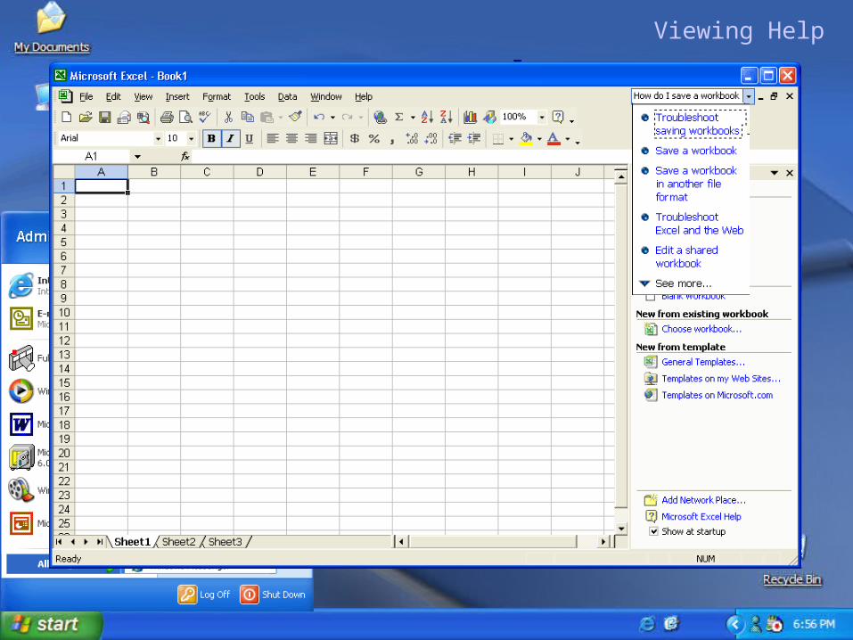
10. Verify that Existing worksheet is selected, and then click OK.

11. On the File menu, click Save.

Importing a Delimited Text File

Importing a Delimited Text File

Querying a Database

To query a database

1. If you have not already done so, open gradebook.xls.

2. Click the Sheet2 tab.

3. Click Data, point to Import External Data, and then click New Database Query.

4. On the Databases tab, click MS Access Database, and then select Use the Query Wizard to create/edit queries. Click OK.

5. Locate the database gradebook.mdb (located in the sample data folder that you downloaded with this tutorial) in the Select Database dialog box, and then click OK. The Query Wizard opens.

6. From the list on the left, click Gradebook, and then click the right arrow. The columns from the database table are now listed on the right.

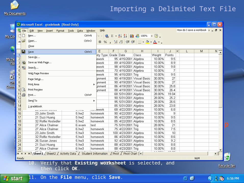
7. If you want to remove any columns from the list, select the appropriate heading, and then click the left arrow.

Querying a DatabaseQuerying a Database

To query a database cont.

8. The Filter Data dialog box allows you to filter the data that you are querying directly from the database. For example, if you wanted to include the records for only grade 5 students, you could do so here. You’ll need to have all the grade book data, so choose not to filter data at this point. Click Next.

9. The Sort Order dialog box allows you to sort the data that you are querying from the database by ascending or descending order. You might want to sort the data later, but choose not to do so here. Click Next.

10. Click Return Data to Microsoft Excel, and then click Finish.

11. Verify that Existing worksheet is selected, and then click OK. Notice that you can also create a PivotTable Report directly from a database query. PivotTables are discussed later in this tutorial. The data from the database opens in Sheet2. The External Data toolbar also appears.

Creating a Web Query

To create a Web Query

1. If you have not already done so, open gradebook.xls.

2. On the Insert menu, click Worksheet.

3. Right-click on the tab of the newly created worksheet, and then click Rename. Name the tab Web Query.

4. On the Data menu, point to Import External Data, and then click New Web Query.

5. Type the address http://www.census.gov/population/socdemo/school/ in the Address box, and then click Go. Scroll down and click tabA-6.txt. The page appears in the New Web Query dialog box.

6. Select the yellow boxes next to the areas of the page you would like in your query. They will turn green when selected. Click Import.

7. Verify that Existing worksheet is selected, and then click OK. The census data is imported into the Excel worksheet.

Creating a Web QueryCreating a Web Query

Filtering a list by Using AutoFilterTo filter a list by using AutoFilter

1. If you have not already done so, open gradebook.xls and then click the Activity Data tab to switch to the appropriate worksheet.

2. Click anywhere in the worksheet to activate a cell.

3. On the Data menu, point to Filter, and then click AutoFilter. Drop-down arrows appear next to the field names in the header row.

4. You can filter the list by values in a single column or in multiple columns. For example, click the drop-down arrow on the Class field, and then click Algebra. The list of activities are reduced to just those that are recorded for the algebra class. Notice that the arrow is blue, indicating that the class is an active part of the filter.

5. In the Activity Type drop-down menu, click homework to view recorded homework grades. You can filter by any combination of columns.

6. Select row 43 by clicking 43 in the row headings on the left side of the worksheet.

7. On the Insert menu, click Rows to insert a new row above row 43.

8. Fill in a homework activity for Suzi Huang. Her student ID is 21. To fill in the remaining parts, select cells B23 to J23, click the fill handle at the lower right corner of cell J23 and drag to fill in row 43. Lastly, change Suzi’s grade for the activity to 88.

Filtering a List by Using AutoFilter

Filtering a List by Using AutoFilter

Weighting Activities and Dropping the Lowest Grade

To weight activities and drop the lowest grade

1. Switch to the Pivot worksheet by clicking on the appropriate tab at the bottom of the screen.

2. Click in cell K7 and type ’=’ to indicate to Excel that you are entering a formula.

3. Type MIN( and select all the scores for homework (D7:F7) and close the parenthesis. The formula should read ‘=MIN(D7:F7)’. Notice the range you have typed is highlighted in blue in the sheet to the left. Press Enter. You have computed the lowest grade for homework.

4. Click in cell L7 and type the formula to calculate the overall homework grade now that you’ve dropped the lowest one. The formula is ‘=(SUM(D7:F7)-K7)/2’. Press Enter. This gets a total homework score (SUM(D&:F7), subtracts the lowest score (-K7), and then divides by the number of homework grades that remain (/2).

5. Click in cell M7, type ‘=SUM(G8:I8,C8)+L7*0.3’, and then press Enter. This represents the sum of all the weighted points for activities excluding the homework (SUM(G8:I8,C8), plus the calculated homework score (L7) multiplied by the weight for the overall homework grade (*0.3) of 30%. This gives you a final score for Rolfie of 87.94.

Weighting Activities and Dropping the Lowest Grade

Weighting Activities and Dropping the Lowest Grade

Using Vlookup to Assign Letter Grades to Scores

Using Vlookup to Assign Letter Grades to Scores

Using Vlookup to Assign Letter Grades to Scores

To use Vlookup to assign letter grades to scores

1. Change to the Score worksheet by clicking on the tab at the bottom of the screen. You might have to scroll through the tabs to the right by using the worksheet tab navigation buttons in the lower left corner.

2. Switch to the Pivot worksheet by clicking on the appropriate tab at the bottom of the screen.

3. Click in cell N7, type ‘=VLOOKUP(M7,Score!$A$1:$B$6,2)’, and then press Enter. In this formula, we are finding the value of M7 exists in the scale provided on the score sheet. Because the value 87 is between 80 and 90, the function selects the next lower value (80). Then the corresponding value to 80 in the 2nd column is returned. The middle section of the formula that reads (Score!$A$1:$B$6) tells the function to look at the sheet named Score and always look to the range from A1 to B6 to find the values. If you expand the list in the Score sheet, you will need to modify this part to reflect the change.

4. The value now in N7 is B and if you look at the grading scale, a B would be correct for an 87.

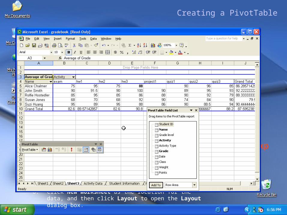
Creating a PivotTable

To create a PivotTable

1. If you have not already done so, open gradebook.xls and then click the Activity Data tab to activate the Activity Data worksheet. To remove the Autofilter, on the Data menu, click Filter, and then click Autofilter if the filter is on.

2. Select cell J43 to cell A1.

3. On the Data menu, click PivotTable and PivotChart Report. The PivotTable and PivotChart Wizard open.

4. Click Microsoft Excel List or database as the location of the data to analyze, and then click PivotTable. Click Next.

5. Because you have already selected the worksheet (step 2), the correct data range should be entered in the Range field. (The range is surrounded by a pulsing dashed line.) Click Next. If the data is not selected, click Cancel and return to step 2.

6. Click New Worksheet as the location for the data, and then click Layout to open the Layout dialog box.

Creating a PivotTableCreating a PivotTable

To create a PivotTable cont.

7. You can ask different questions of the data and look at it in different ways depending on which fields you decide to use for rows, columns, and data. For example, if you want to see the sheet as you might a page in a traditional paper grade book, drag the Name field to the Row box on the PivotTable diagram. Drag the Activity field to the Column box. Drag the Grade field to the Data box. (Note: you can use the same field in more than one place.)

8. When you are finished, click OK, and then click Finish. The PivotTable opens and the PivotTable toolbar and Field List appear.

9. Double-click Sum of Grade in the upper-left corner of the PivotTable, click Average, and then click OK. This way the grades are averaged instead of added.

Creating and Customizing a PivotChart

Creating and Customizing a PivotChart

Creating and Customizing a PivotChart

To create and customize a PivotChart

1. Click the Chart Wizard button on the PivotTable toolbar. The default chart type will open on a separate Chart worksheet.

2. To change the chart type, click the Chart Wizard button on the PivotTable toolbar again. (Notice that the shortcut menu on the toolbar is now labeled PivotChart instead of PivotTable.) The Chart Wizard opens.

3. Select from one of the standard or custom chart types, and then click Next.

4. In the Chart Options dialog box, you can give the chart a title, show or hide gridlines, change the placement of the chart legend, change data labels, and show a data table with your chart.

5. The Chart Location dialog box allows you to select a location for your PivotChart, as a separate worksheet or embedded in your PivotTable report.

6. Click Finish to display your PivotChart in a new sheet. Remember that as you drag field buttons, your PivotChart automatically updates.

Saving an Excel Worksheet in HTML Format

Saving an Excel Worksheet in HTML Format

Saving an Excel Worksheet in HTML Format

To save an Excel worksheet in HTML format

1. On the File menu, click Save As Web Page.

2. The Save As dialog box allows you to specify whether you want to save the entire workbook or only the active worksheet as a Web page.

3. If you select the active worksheet and you want others to be able to manipulate your data, click Add Interactivity.

4. Click Publish if you want to specify which items in the workbook you want to publish and which type of interactivity you want to add.