Embed Size (px)
Citation preview
OutlineDay 1
1. Introductions– Who am I?– Syllabus– Who are you?
2. Helicopter Tour of Economics– Overview of Micro– Overview of Macro– Other economics we won’t have time for
3. Micro Economics– This morning– This afternoon – CASES!– Tomorrow

IntroductionWho am I?
Tim Simin
– Born in Detroit BUT raised in Dallas, TX
– 1992: Graduated Summa Cum Laude from UTD with BS in Economics and Finance
– 1992 – 1994 : Division of Monetary Affairs at the Federal Reserve Board of Governors in Washington, D.C.
– 1995 – 2000: Ph.D. in Finance from the University of Washington
– 2000 – Today: Assoc. professor of Finance, Smeal College of Business, Penn State
– Course taught
– Research

IntroductionsSyllabus
1. Download it (for now) at http://timsimin.net/UT/
2. Schedule
3. Please contact me via email about scheduling, homework, or other problems
IntroductionsWho are you?
Write down on regular sized piece of paper:
– Name
– Current Job, i.e. company and position Be specific please
– Expertise
– Economic background Senior Economist Some undergrad economics Took home economics in high school I abhor economics
– Anything else you want me to know about you Nickname, etc.
Helicopter TourWhat is economics?
1. Wikipedia: – Economics is the social science that analyzes the production,
distribution, and consumption of goods and services
2. Most economics based on the idea that agents are rational
3. Most economics can be summed up by saying, “People respond to incentives” - Landsberg
4. A “positive” rather than “normative” science– Not a science of what is right or wrong, only what the outcome
will be given some action– May be morally offensive
Helicopter TourWhat Microeconomics?
Microeconomics covers:– Price determination via quantities supplied and demanded
Laws of demand
– Opportunity costs and sunk costs
– Theory of the firm Monopolies, Oligopolies, and perfect competition Cost benefit analysis/profit maximization
– Theory of the consumer Utility functions, budget constraints, utility maximization
– Specialization, efficiency, comparative advantage
– Examples
Helicopter TourWhat is Macroeconomics?
Macroeconomics covers:
– Fiscal policy http://www.wtfnoway.com/ and http://www.usdebtclock.org/
– Monetary policy
– National Income Accounting GNP, GDP
– Interest rate determination
– Exchange rate determination
– Business Cycles
– Inflation
Helicopter TourWhat Else is in economics?
1. Game theory– Models of strategic interaction between agents
Prisoner’s dilemma
2. Finance– The economics of how companies choose and finance projects– The economics of how financial asset prices are determined
3. Law and Economics– Coase theorems
4. Behavioral Economics– People are NOT rational but behave according to documented
psychological biases
Game TheoryThe game of dilemmas
1. Consider a non-cooperative duopoly trying to figure out what price to charge for a homogeneous good. Both firms can pick between just two prices, a high price, $10 or a low price, $6
2. If firm 1 charges the high price and firm 2 also charges a high price their profits will be $1000.
3. If firm 1 charges a high price and firm 2 charges a low price then firm two will get more business and the profits of firm 1 will be $0 and firm 2 will make $1500.
4. Now if both firms charge the low price then each firm will only make $300.
5. Let’s look at a picture of these assumptions.
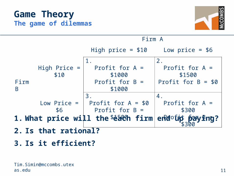
1. What price will the each firm end up paying?
2. Is that rational?
3. Is it efficient?
Firm A
High price = $10 Low price = $6
Firm B
High Price = $101.
Profit for A = $1000Profit for B = $1000
2.Profit for A = $1500
Profit for B = $0
Low Price = $63.
Profit for A = $0Profit for B = $1500
4.Profit for A = $300Profit for B = $300
Game TheoryThe game of dilemmas
IntroductionSome definitions
1. Models – A filter for reality
– Don’t attack assumptions only how well it fits reality
2. Opportunity cost:
– Value of the next best alternative
– Sum of explicit and implicit costs
3. Positive vs. Normative analysis:– Positive analysis = scientific or objective
– Normative analysis = moral or value judgment
IntroductionSome definitions
1. Rationality:
– What is rational behavior?
– “Most of economics can be summarized in four words: ‘People respond to incentives.’ The rest is commentary.” - Landsberg
– This assumption brings up many questions of seemingly “irrational” behavior Why do people vote? Why do people buy insurance when they rent a car even
though their car insurance or credit card already provides them coverage?
Why do people buy actively managed mutual funds?
DemandTypes of demand
1. Demand (Qd)
– Amount of a good consumers are willing to buy at a given price and over a given period of time
– Not how much a consumer wants or desires a good
2. Two types of demand functions
– Generalized demand
Many different things affect quantity demanded
– Ordinary demand
Only price affects Qd. Price is the most important factor
DemandDeterminants of demand
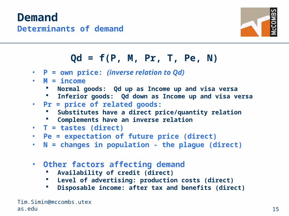
Qd = f(P, M, Pr, T, Pe, N)
• P = own price: (inverse relation to Qd)• M = income
Normal goods: Qd up as Income up and visa versa Inferior goods: Qd down as Income up and visa versa
• Pr = price of related goods: Substitutes have a direct price/quantity relation Complements have an inverse relation
• T = tastes (direct)• Pe = expectation of future price (direct)• N = changes in population - the plague (direct)
• Other factors affecting demand Availability of credit (direct) Level of advertising: production costs (direct) Disposable income: after tax and benefits (direct)
DemandGeneralized vs. Ordinary
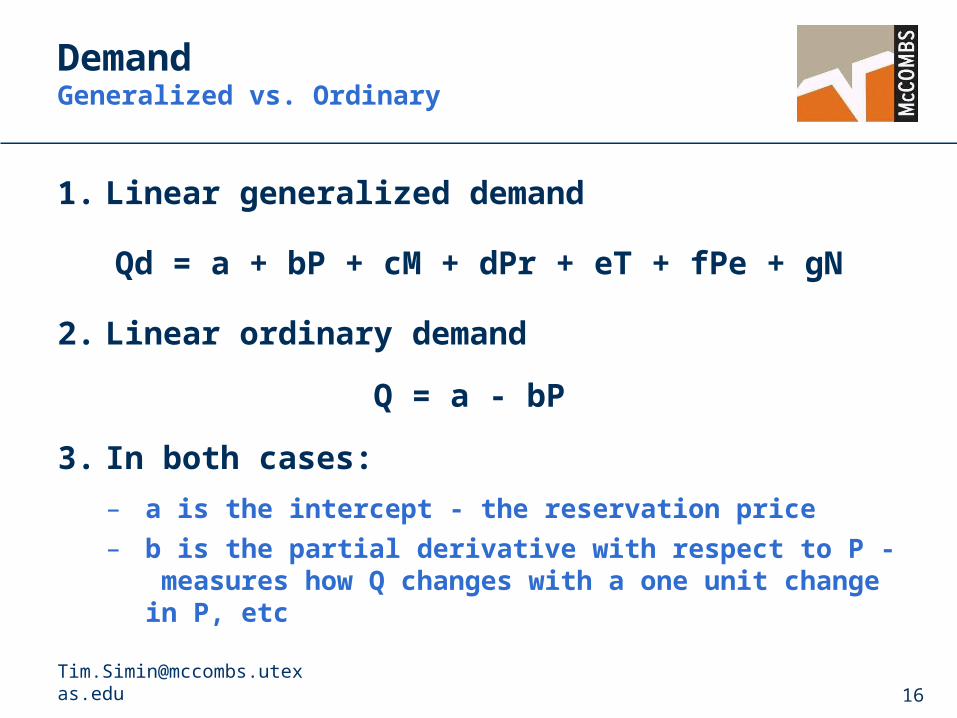
1. Linear generalized demand
Qd = a + bP + cM + dPr + eT + fPe + gN
2. Linear ordinary demand
Q = a - bP
3. In both cases:
– a is the intercept - the reservation price
– b is the partial derivative with respect to P - measures how Q changes with a one unit change in P, etc
DemandLinear generalized demand function
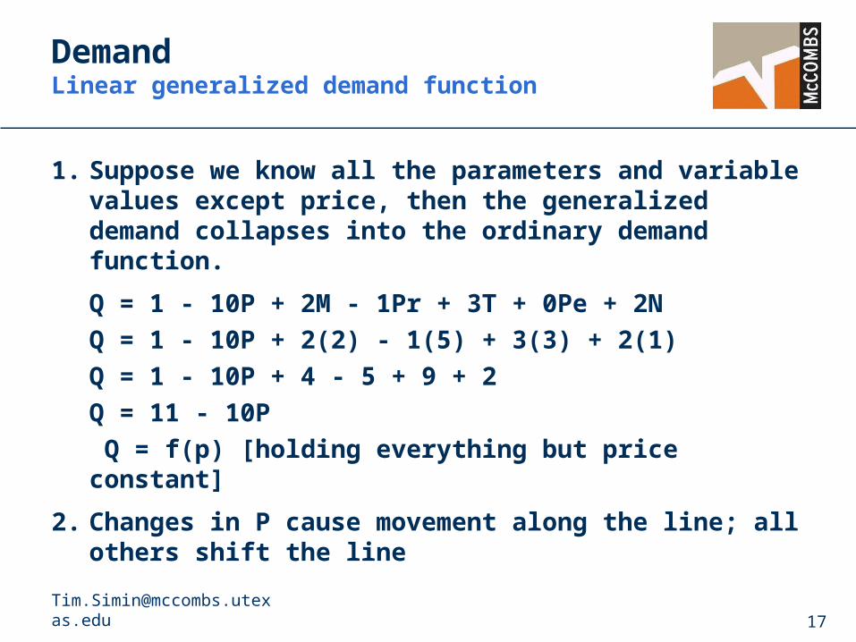
1. Suppose we know all the parameters and variable values except price, then the generalized demand collapses into the ordinary demand function.
Q = 1 - 10P + 2M - 1Pr + 3T + 0Pe + 2N
Q = 1 - 10P + 2(2) - 1(5) + 3(3) + 2(1)
Q = 1 - 10P + 4 - 5 + 9 + 2
Q = 11 - 10P
Q = f(p) [holding everything but price constant]
2. Changes in P cause movement along the line; all others shift the line
DemandThe First Law of Demand
1. First Law of Demand:
– The price of a good is inversely related to the quantity demanded ceteris paribus. Normally, as the price of a good increases the quantity demanded decreases.
2. Difference between “demand” and “quantity demanded”
– Demand refers to the whole curve.
– Quantity demanded refers to points (movements) along the curve.
3. Incentives - a justification for the First Law of Demand
– Example: Do seat belt and helmet laws reduce the number of injuries that occur while driving?
SupplyDeterminants of supply
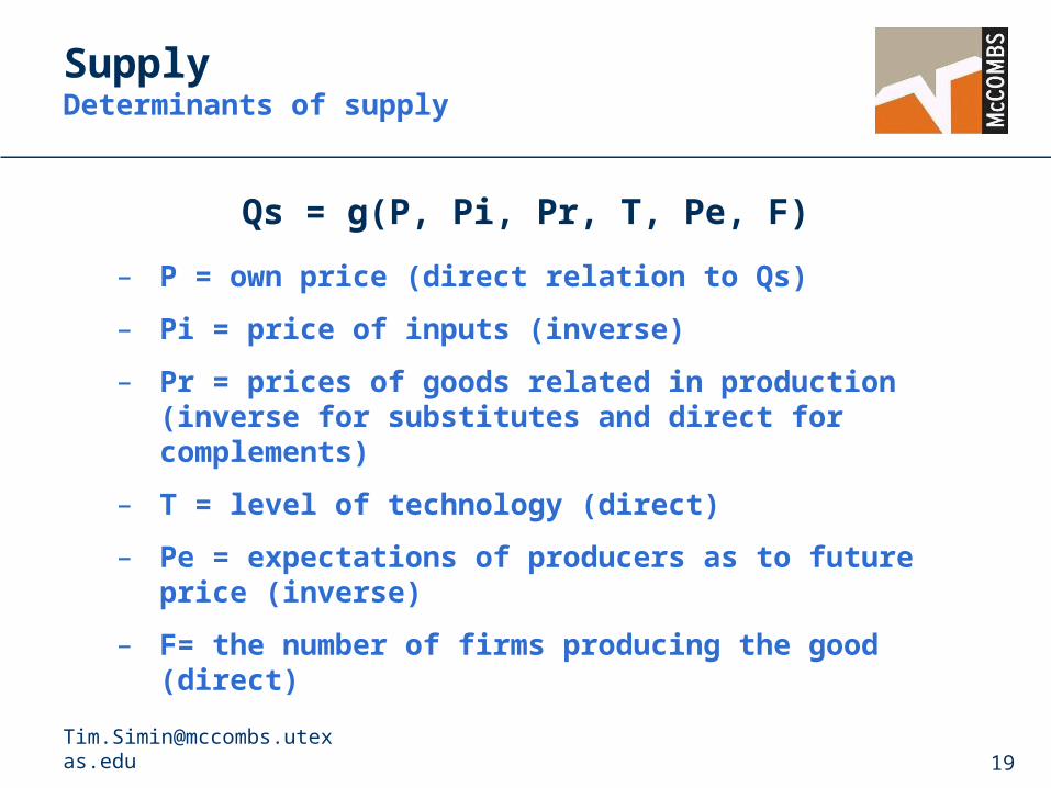
Qs = g(P, Pi, Pr, T, Pe, F)
– P = own price (direct relation to Qs)
– Pi = price of inputs (inverse)
– Pr = prices of goods related in production (inverse for substitutes and direct for complements)
– T = level of technology (direct)
– Pe = expectations of producers as to future price (inverse)
– F= the number of firms producing the good (direct)
Market EquilibriumEquilibrium, excess supply, excess demand
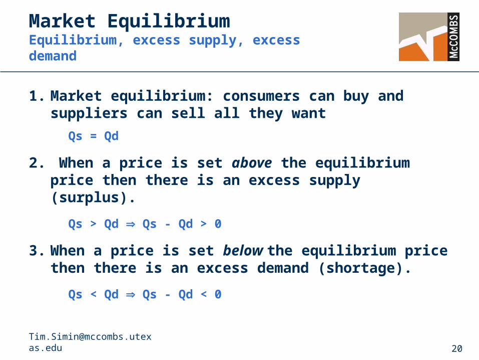
1. Market equilibrium: consumers can buy and suppliers can sell all they want
Qs = Qd
2. When a price is set above the equilibrium price then there is an excess supply (surplus).
Qs > Qd Qs - Qd > 0
3. When a price is set below the equilibrium price then there is an excess demand (shortage).
Qs < Qd Qs - Qd < 0
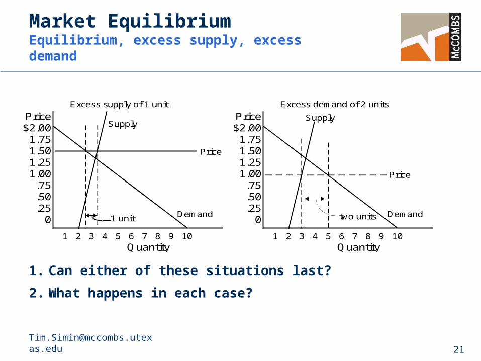
Market EquilibriumEquilibrium, excess supply, excess demand
1. Can either of these situations last?
2. What happens in each case?
Price$2.001.751.501.251.00.75.50.25
0
1 2 3 4 5 6 7 8 9 10Quantity
Excess supply of 1 unit
Demand
Supply
Price
1 unit
Price$2.001.751.501.251.00.75.50.25
0
1 2 3 4 5 6 7 8 9 10Quantity
Excess demand of 2 units
Demand
Supply
Price
two units
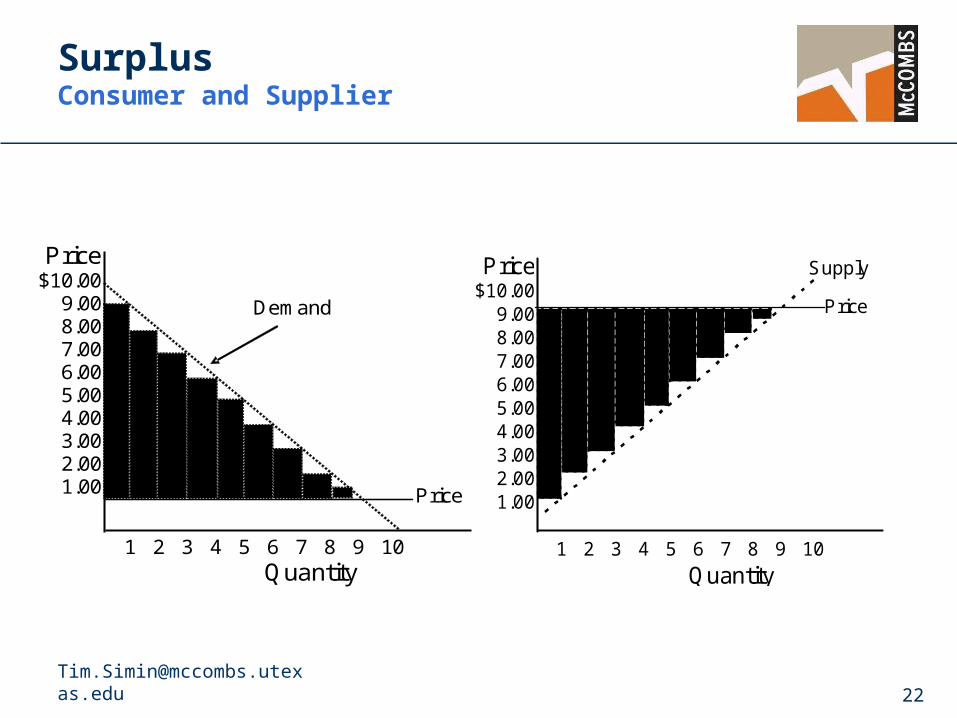
SurplusConsumer and Supplier
Price $10.00
9.00 8.00 7.00 6.00 5.00 4.00 3.00 2.00 1.00
1 2 3 4 5 6 7 8 9 10 Quantity
Price
Demand
Price$10.00
9.008.007.006.005.004.003.002.001.00
1 2 3 4 5 6 7 8 9 10
Quantity
Price
Supply
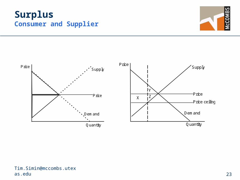
SurplusConsumer and Supplier
Price
Demand
Price
Quantity
Supply
Price
Demand
Price
Quantity
Supply
Price ceiling X
Y
Z
Elasticity, TR, and MRElasticity
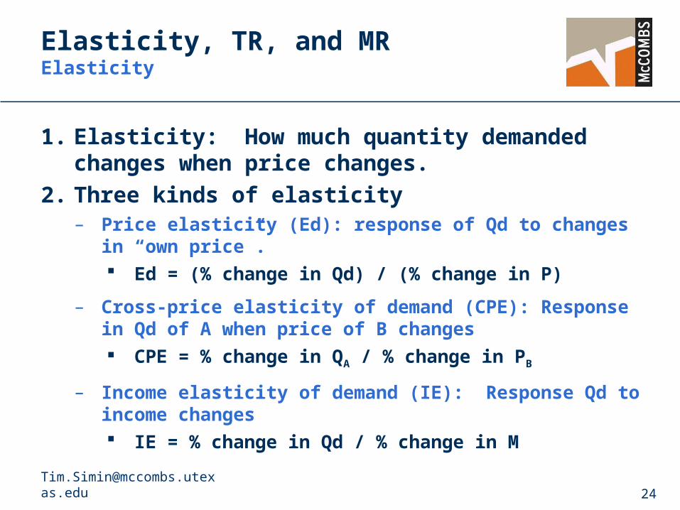
1. Elasticity: How much quantity demanded changes when price changes.
2. Three kinds of elasticity– Price elasticity (Ed): response of Qd to changes in “own price”.
Ed = (% change in Qd) / (% change in P)
– Cross-price elasticity of demand (CPE): Response in Qd of A when price of B changes
CPE = % change in QA / % change in PB
– Income elasticity of demand (IE): Response Qd to income changes IE = % change in Qd / % change in M
Elasticity, TR, and MRPrice elasticity
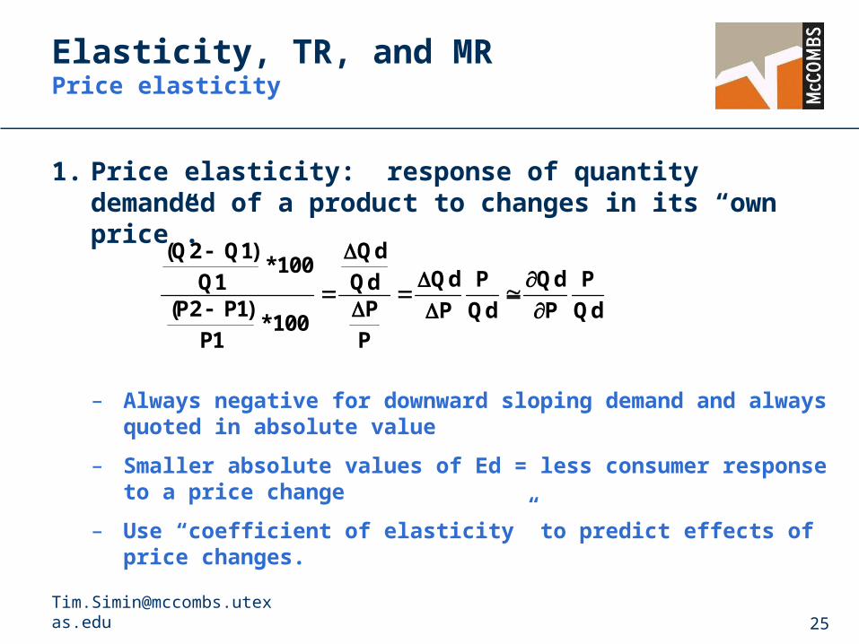
1. Price elasticity: response of quantity demanded of a product to changes in its “own price”.
– Always negative for downward sloping demand and always quoted in absolute value
– Smaller absolute values of Ed = less consumer response to a price change
– Use “coefficient of elasticity” to predict effects of price changes.
( )*
( )*
Q Q
QP P
P
Qd
QdP
P
Qd
P
P
Qd
Qd
P
P
Qd
2 1
1100
2 1
1100
Elasticity, TR, and MRPrice elasticity
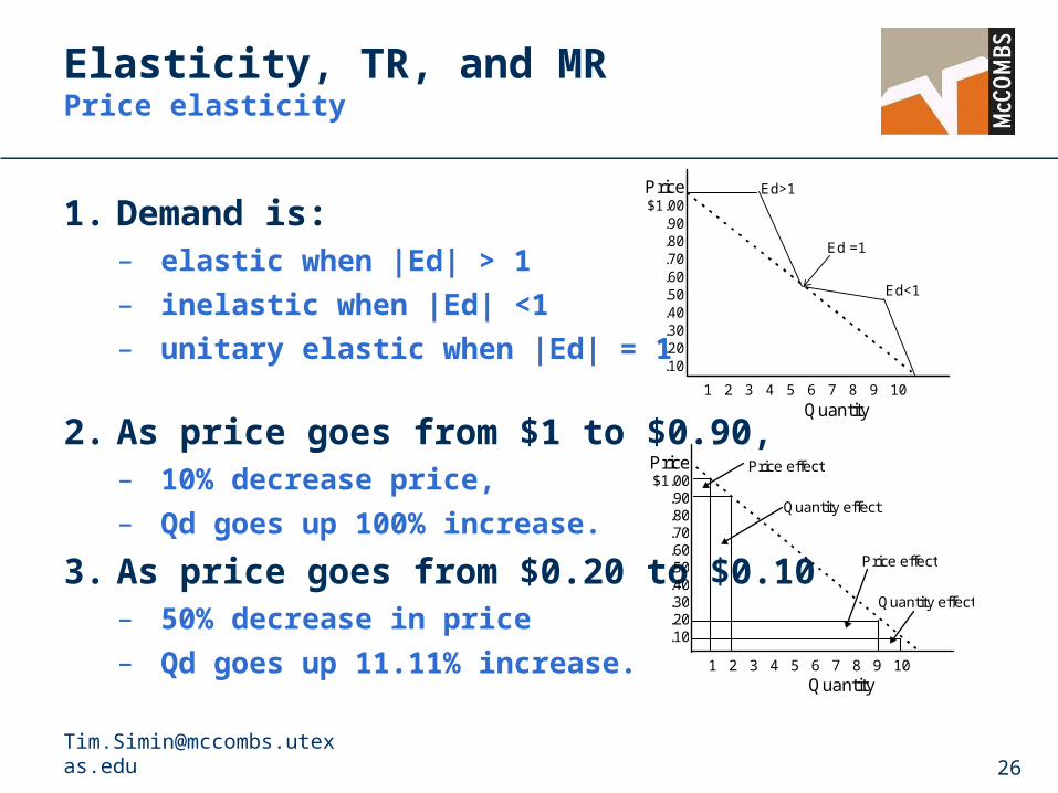
1. Demand is:– elastic when |Ed| > 1
– inelastic when |Ed| <1
– unitary elastic when |Ed| = 1
2. As price goes from $1 to $0.90, – 10% decrease price,
– Qd goes up 100% increase.
3. As price goes from $0.20 to $0.10 – 50% decrease in price
– Qd goes up 11.11% increase.
Ed<1
Price$1.00
.90
.80
.70
.60
.50
.40
.30
.20
.10
1 2 3 4 5 6 7 8 9 10
Quantity
Ed>1
Ed =1
Price$1.00
.90
.80
.70
.60
.50
.40
.30
.20
.10
1 2 3 4 5 6 7 8 9 10Quantity
Price effect
Quantity effect
Quantity effect
Price effect
Elasticity, TR, and MRPrice elasticity
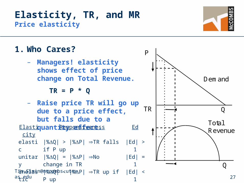
1. Who Cares?
– Managers! elasticity shows effect of price change on Total Revenue.
TR = P * Q
– Raise price TR will go up due to a price effect, but falls due to a quantity effect.
Elasticity Responsiveness Ed
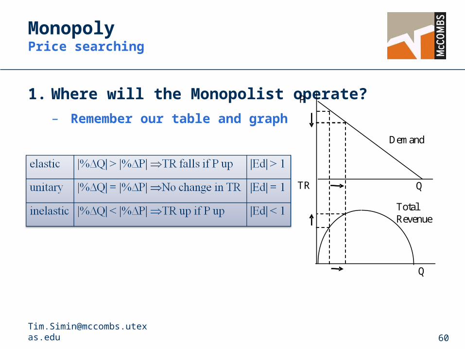
elastic |%Q| > |%P| TR falls if P up |Ed| > 1
unitary |%Q| = |%P| No change in TR |Ed| = 1
inelastic |%Q| < |%P| TR up if P up |Ed| < 1
TR
Q
Q
P
Demand
Total Revenue
Elasticity, TR, and MRMarginal revenue
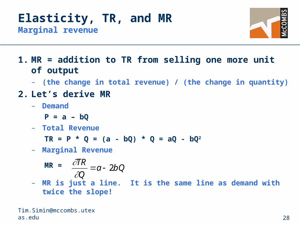
1. MR = addition to TR from selling one more unit of output– (the change in total revenue) / (the change in quantity)
2. Let’s derive MR– Demand
P = a – bQ
– Total Revenue
TR = P * Q = (a - bQ) * Q = aQ - bQ2
– Marginal Revenue
MR =
– MR is just a line. It is the same line as demand with twice the slope!
bQaQ
TR2
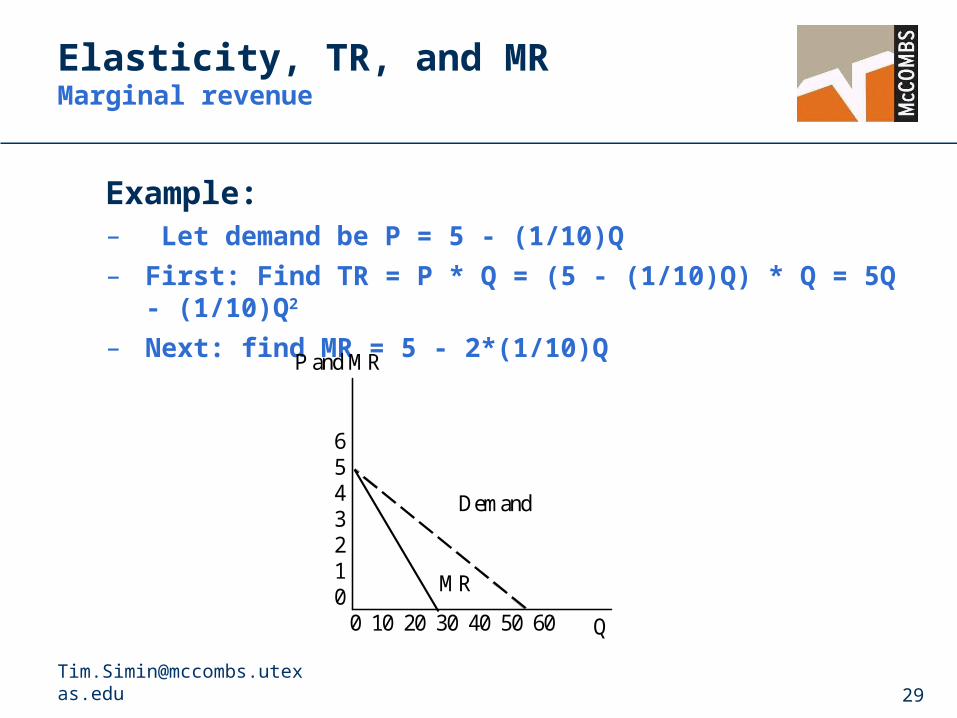
Elasticity, TR, and MRMarginal revenue
Example: – Let demand be P = 5 - (1/10)Q
– First: Find TR = P * Q = (5 - (1/10)Q) * Q = 5Q - (1/10)Q2
– Next: find MR = 5 - 2*(1/10)Q
Q
P and MR
0 10 20 30 40 50 60
6 5 4 3 2 1 0
MR
Demand
Elasticity, TR, and MRRelating all three
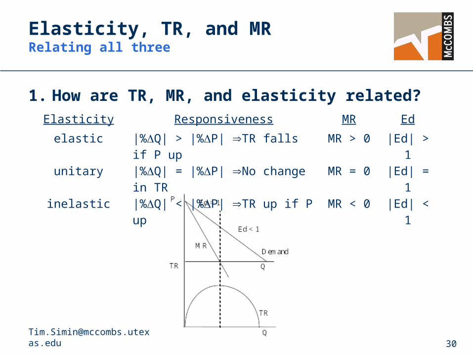
1. How are TR, MR, and elasticity related?
Elasticity Responsiveness MR Ed
elastic |%Q| > |%P| TR falls if P up MR > 0 |Ed| > 1
unitary |%Q| = |%P| No change in TR MR = 0 |Ed| = 1
inelastic |%Q| < |%P| TR up if P up MR < 0 |Ed| < 1
OptimizationConcepts and terms
1. Objective function: function to maximize or minimize.– Managers maximize profits or sales or minimize costs
– Consumers maximize utility or satisfaction
2. Choice variables: variables that when changed affect value of objective
– If objective is profit, then a choice variable is quantity.
– If objective is cost, then a choice variable is expenditures.
– If objective is utility, then a choice variable is amount of a good
3. Unconstrained and constrained maximization
4. Why is marginal analysis so important?
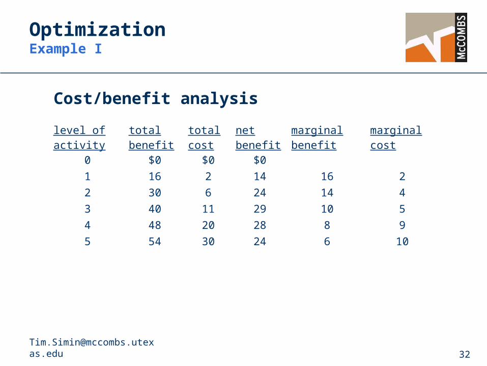
OptimizationExample I
Cost/benefit analysis
level of activity total benefit total cost net benefit marginal benefit marginal cost
0 $0 $0 $0
1 16 2 14 16 2
2 30 6 24 14 4
3 40 11 29 10 5
4 48 20 28 8 9
5 54 30 24 6 10
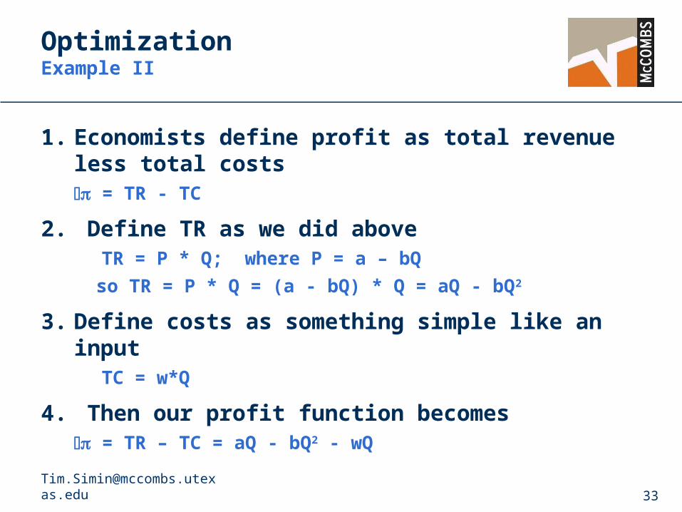
OptimizationExample II
1. Economists define profit as total revenue less total costs = TR - TC
2. Define TR as we did aboveTR = P * Q; where P = a – bQ
so TR = P * Q = (a - bQ) * Q = aQ - bQ2
3. Define costs as something simple like an input TC = w*Q
4. Then our profit function becomes = TR – TC = aQ - bQ2 - wQ
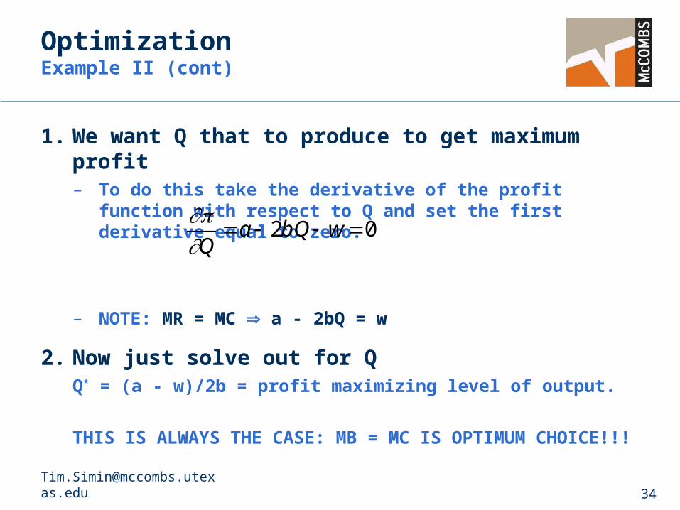
OptimizationExample II (cont)
1. We want Q that to produce to get maximum profit– To do this take the derivative of the profit function with respect to
Q and set the first derivative equal to zero.
– NOTE: MR = MC a - 2bQ = w
2. Now just solve out for Q Q* = (a - w)/2b = profit maximizing level of output.
THIS IS ALWAYS THE CASE: MB = MC IS OPTIMUM CHOICE!!!
02 wbQaQ
Consumer behaviorSome definitions
1. Rational behavior: – Consistent with behavior postulates and preference axioms
2. Behavior Postulates: – Statement without proof – usually obvious or well known
3. Preference axioms: – How people deal with ranking preferences
4. Utility: – Ranking of preferences or a measure of happiness. More
preferred goods or bundles of goods have a higher utility
5. Utility Maximization: – Trying to get most preferred bundle of goods they can afford
Consumer behaviorIndifference Curves (IC’s)
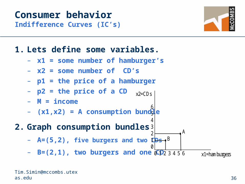
1. Lets define some variables. – x1 = some number of hamburger’s
– x2 = some number of CD’s
– p1 = the price of a hamburger
– p2 = the price of a CD
– M = income
– (x1,x2) = A consumption bundle
2. Graph consumption bundles
– A=(5,2), five burgers and two CDs
– B=(2,1), two burgers and one CD
x1=hamburgers
x2=CDs
A B
0 1 2 3 4 5 6
6 5 4 3 2 1 0
Consumer behaviorIndifference Curves (cont)
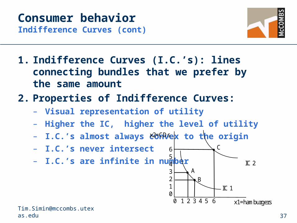
1. Indifference Curves (I.C.’s): lines connecting bundles that we prefer by the same amount
2. Properties of Indifference Curves:– Visual representation of utility
– Higher the IC, higher the level of utility
– I.C.’s almost always convex to the origin
– I.C.’s never intersect
– I.C.’s are infinite in number
x1=hamburgers
x2=CDs
A
B
0 1 2 3 4 5 6
6 5 4 3 2 1 0
IC 1
C
IC 2
Consumer behaviorIndifference Curves (cont)
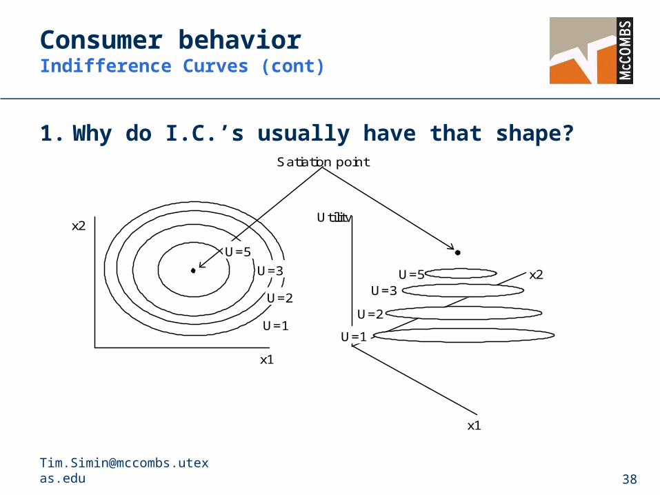
1. Why do I.C.’s usually have that shape?
x1
x2
Utility
Satiation point
x1
x2
U=1
U=2
U=3
U=5
U=5U=3
U=2
U=1
Consumer behaviorIndifference Curves (cont)
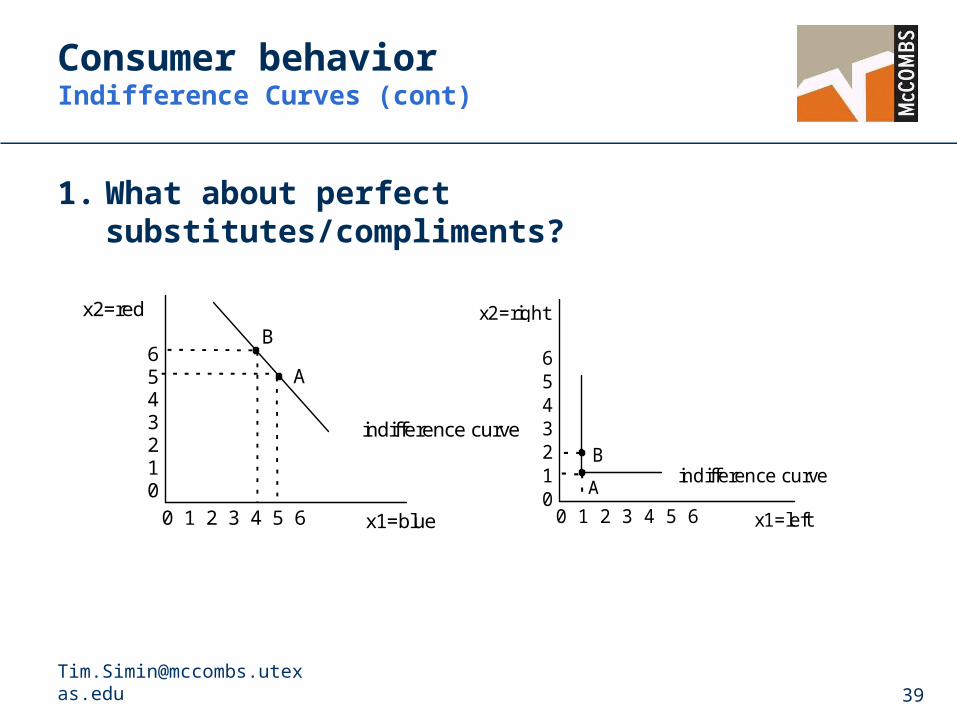
1. What about perfect substitutes/compliments?
x1=blue
x2=red
A
B
0 1 2 3 4 5 6
6543210
indifference curve
x1=left
x2=right
A
B
0 1 2 3 4 5 6
6543210
indifference curve
Consumer behaviorBudget lines
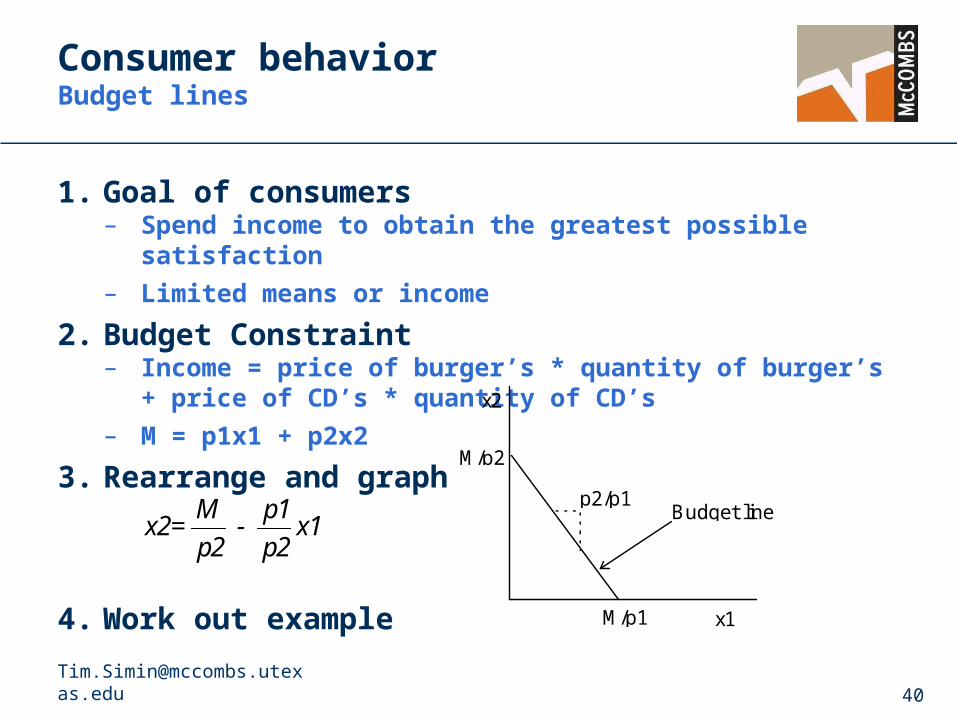
1. Goal of consumers– Spend income to obtain the greatest possible satisfaction
– Limited means or income
2. Budget Constraint– Income = price of burger’s * quantity of burger’s + price of CD’s
* quantity of CD’s
– M = p1x1 + p2x2
3. Rearrange and graph
4. Work out example
M p1x2= - x1
p2 p2
x1
x2
M/p1
M/p2
Budget linep2/p1
Utility MaximizationPutting it all together
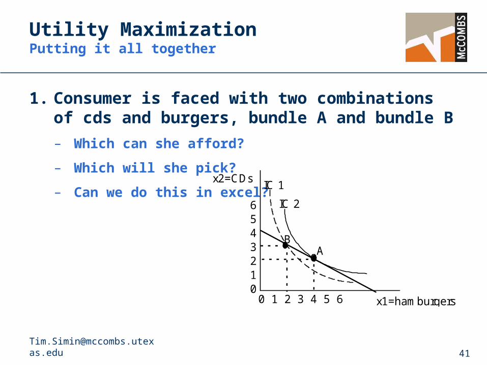
1. Consumer is faced with two combinations of cds and burgers, bundle A and bundle B
– Which can she afford?
– Which will she pick?
– Can we do this in excel?
x1=hamburgers
x2=CDs
AB
0 1 2 3 4 5 6
6543210
IC 1
IC 2
Production Theory Costs and Product
1. Production Theory: – How firms deal with inputs in production and costs of inputs
– Notes: Short run vs. Long run Assume firm produces a product rather than a service
2. The Producer’s Problem: – Producers want to be efficient
maximize output subject to costs of production OR minimize costs subject to an output level.
– Two kinds of efficiency technical efficiency economic efficiency
Production Theory Costs and Product (cont)
1. Production: – Creation of goods and services from inputs or resources
– Production function: Schedule (table or equation) of max output produced from
specified set of inputs and technology Assuming producers are technically efficient (not wasteful) Really dealing with economic efficiency
2. Two views of the producer problem:– Find optimal level of output given a cost function
Solve the profit max problem
– Find the most efficient means of producing a given level of output Constrained minimization problem with production function
being the objective function and an output the constraint
Production Theory Total Product
1. Total Product: fancy name for output (Q)
Q = f(I1, I2, I3, ...)– Land– labor (L)– capital (K)– entrepreneurial ability
2. There are two different types of inputs– Fixed inputs
These can be changed only in the long run– Variable inputs
3. Restrict ourselves to L and K for simplicity
Production Theory Total Product (cont)
4. The general production function will be Q = f(L,K)– Specific forms of typical production functions
Multiplicative: Q=LKCubic: Q=aK3L3+bK2L2Cobb-Douglas: Q=KL
Additive: Q=wL+rK
5. Three aspects of short run production
– Total product: TP = Q=f(L,K)– Average product AP = Q/L– Marginal product MP = Q/L
6. Fix K to examine short-run production
Production Theory Example
1. Cubic production: Q=aK3L3+bK2L2
– Let a = -.1 and b = 3.
2. See excel sheet
3. Note shapes of curves– TP increases and then falls back down right around 10 people.
– AP is maximized at 44.8, somewhere between 7 and 8 people.
– MP (the additional output coming from adding one more worker), actually goes negative at the 11th worker.
– MP = 0 when TP is maximized. Why?
4. Why do the curves have these shapes? – Law of diminishing marginal product: As variable input
increases, ceteris paribus, a point will be reached where mp falls
Using TP, AP, MP What can we do with this stuff
1. Assume the following production function: Q=2L.3K.7
– Make a short run decision about how many people to hire to produce 20 units. Fix our capital input at 8.
– In the long run, we can increase our capital input to 12. How many people will we need working for us to produce 20 units?
– What does AP do for us? Not much really. It is just the average amount of output per
worker, given a particular K.
– What does MP do for us? How much more output we get for one more unit of input. Back to our original scenario with k=8. What is MP? Is the Law of diminishing marginal product at work here?
CostsA rose by any other name…
1. Opportunity costs: The value of the next best alternative
– Consist of two different parts
Explicit costs: Out of pocket expense or monetary expense.
Implicit costs: Forgone return had the owners used their resources in the next best use.
– These are both real costs!
2. Example: Consider two companies exactly the same in every way except one rents the building and the other owns the building it operates in. Are their costs different?
CostsTotal, fixed, and variable
1. Short Run Costs:– Total costs = Fixed costs + Variable costs
TC = FC + VC
– Fixed costs: must be paid whether we produce or not (I.E. Rent, Debt payments)
– Variable costs: Costs which change with level of output (I.E. Cost of inputs, Wages) Can break down these costs too.
• Average fixed costs = FC/Q• Average variable costs = VC/Q
– Short Run Marginal Costs = TC/Q = the derivative of TC SMC is additional cost for next unit of output In the short run fixed costs are constant so = (VC/Q)
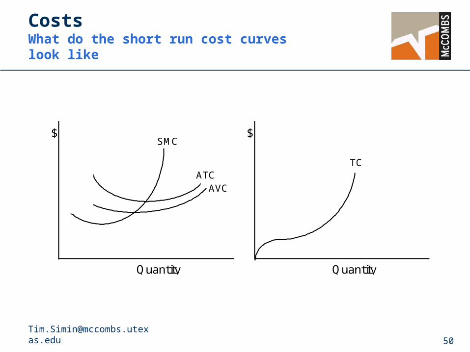
Costs What do the short run cost curves look like
$
Quantity
AVCATC
SMC$
Quantity
TC
CostsRelation to production
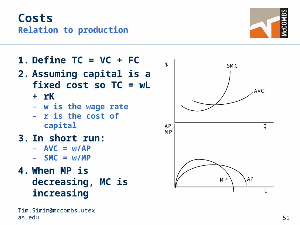
1. Define TC = VC + FC
2. Assuming capital is a fixed cost so TC = wL + rK – w is the wage rate– r is the cost of capital
3. In short run:– AVC = w/AP– SMC = w/MP
4. When MP is decreasing, MC is increasing
$
L
AP, MP
Q
MP AP
AVC
SMC
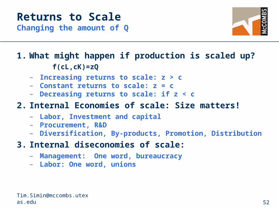
Returns to ScaleChanging the amount of Q
1. What might happen if production is scaled up? f(cL,cK)=zQ
– Increasing returns to scale: z > c – Constant returns to scale: z = c– Decreasing returns to scale: if z < c
2. Internal Economies of scale: Size matters!– Labor, Investment and capital– Procurement, R&D– Diversification, By-products, Promotion, Distribution
3. Internal diseconomies of scale:– Management: One word, bureaucracy– Labor: One word, unions
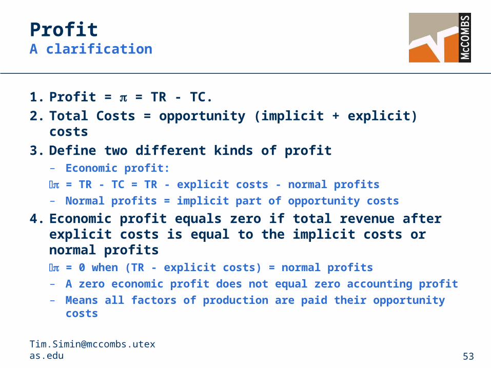
ProfitA clarification
1. Profit = = TR - TC.
2. Total Costs = opportunity (implicit + explicit) costs
3. Define two different kinds of profit– Economic profit:
= TR - TC = TR - explicit costs - normal profits
– Normal profits = implicit part of opportunity costs
4. Economic profit equals zero if total revenue after explicit costs is equal to the implicit costs or normal profits = 0 when (TR - explicit costs) = normal profits
– A zero economic profit does not equal zero accounting profit
– Means all factors of production are paid their opportunity costs
Theory of the FirmThe Perfectly Competitive Model of a Firm
1. Perfect Competition:– Large number of small firms.
– Homogeneous products (Perfect substitutes)
– No single firm can affect the price - firms are price takers
– Each firm can sell all the output it produces at the current market price - the demand curve is perfectly elastic
– Entry and exit are unrestricted
– All firms have perfect information of the production and market for this product
– Managers are profit maximizers
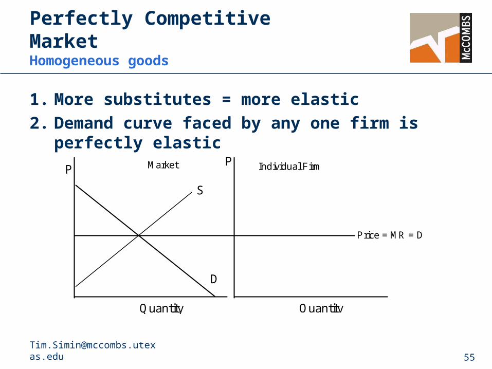
Perfectly Competitive MarketHomogeneous goods
1. More substitutes = more elastic
2. Demand curve faced by any one firm is perfectly elastic
P
Quantity
Individual FirmP
Quantity
Market
Price = MR = D
D
S
Perfectly Competitive FirmGraphical model
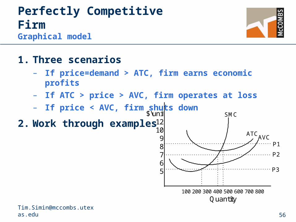
1. Three scenarios– If price=demand > ATC, firm earns economic profits
– If ATC > price > AVC, firm operates at loss
– If price < AVC, firm shuts down
2. Work through examples
$\unit121098765
100 200 300 400 500 600 700 800
Quantity
AVCATC
SMC
P2
P1
P3
Perfectly Competitive Firm Managerial decisions
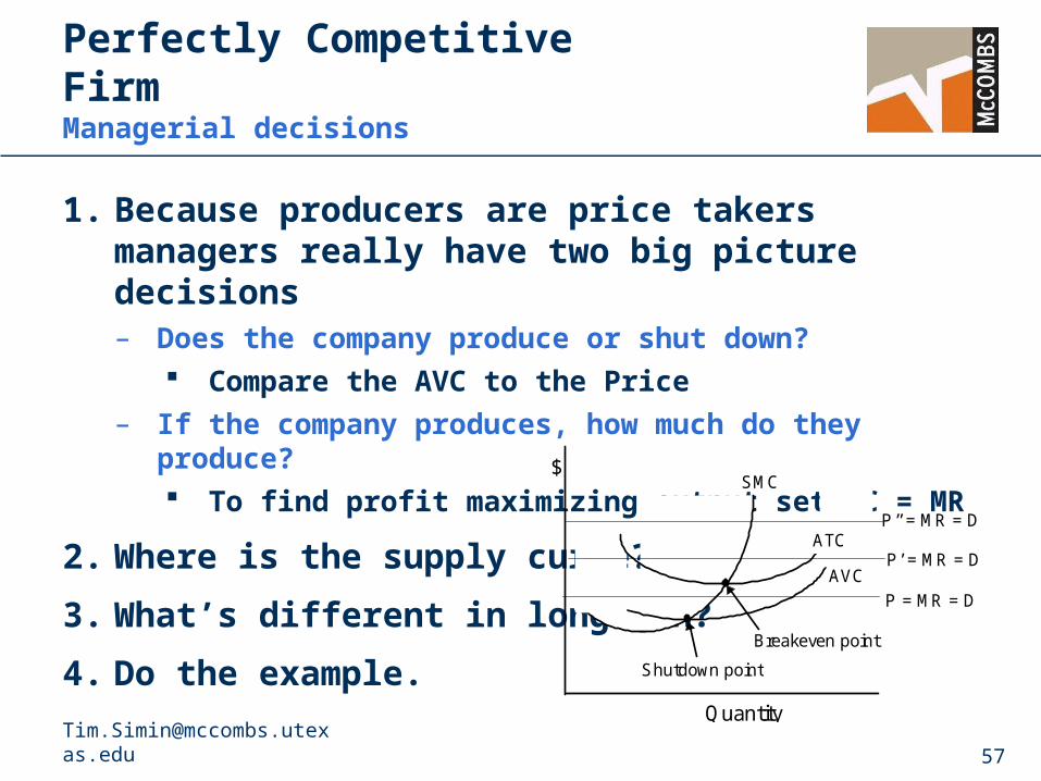
1. Because producers are price takers managers really have two big picture decisions– Does the company produce or shut down?
Compare the AVC to the Price
– If the company produces, how much do they produce? To find profit maximizing output set MC = MR
2. Where is the supply curve?
3. What’s different in long run?
4. Do the example.
$
Quantity
AVC
SMC
P = MR = D
P’ = MR = D
P’’ = MR = DATC
Shutdown point
Breakeven point
Market Power Monopolies
1. Market power: change price without losing all sales
2. Monopolies: produces a good with no close substitute and exists in a market with high barriers to entry – Barriers to entry
Economies of Scale Barriers created by government:
• Licenses: Doctors, Lawyers, Dentists• Patents: Not a guarantee of market power. • Regional franchises: Electricity, Cable television• Regulation: FTC, FDA, FCC, etc.
Input barriers:• Control of raw materials: ALCOA• Capital markets
Brand loyalty
MonopolyGraphical model
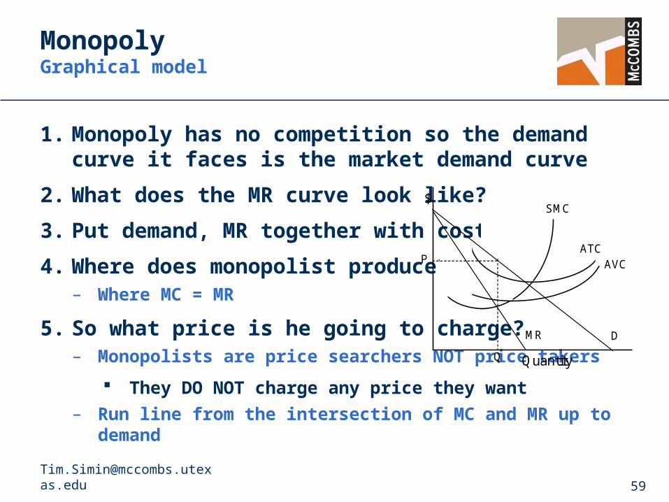
1. Monopoly has no competition so the demand curve it faces is the market demand curve
2. What does the MR curve look like?
3. Put demand, MR together with costs
4. Where does monopolist produce?– Where MC = MR
5. So what price is he going to charge?– Monopolists are price searchers NOT price takers
They DO NOT charge any price they want
– Run line from the intersection of MC and MR up to demand
$
Quantity
AVC ATC
SMC
D MR
P
Q
MonopolyPrice searching
1. Where will the Monopolist operate?
– Remember our table and graph
TR
Q
Q
P
Demand
Total Revenue
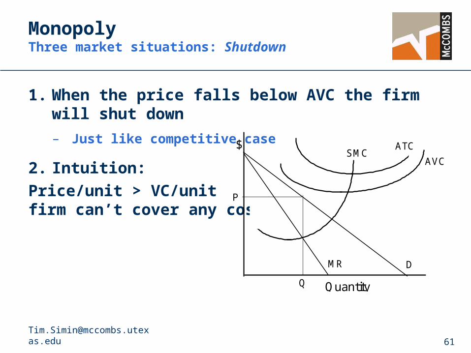
MonopolyThree market situations: Shutdown
1. When the price falls below AVC the firm will shut down
– Just like competitive case
2. Intuition:
Price/unit > VC/unit firm can’t cover any costs
ATC$
Quantity
AVCSMC
DMR
P
Q

MonopolyThree market situations: Operating at a loss
1. When the price falls below ATC but above AVC the firm will operate at a loss
– Just like competitive case
2. Intuition:
FC/unit > Price/unit > VC/unitIf firm shuts down it loses FC sobetter to operate at a loss
$
Quantity
AVCATC
SMC
DMR
P
Q
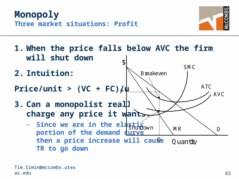
MonopolyThree market situations: Profit
1. When the price falls below AVC the firm will shut down
2. Intuition:
Price/unit > (VC + FC)/unit
3. Can a monopolist really charge any price it wants? – Since we are in the elastic
portion of the demand curve then a price increase will cause TR to go down
$
Quantity
AVCATC
SMC
DMR
P
Q
Shutdown
Breakeven
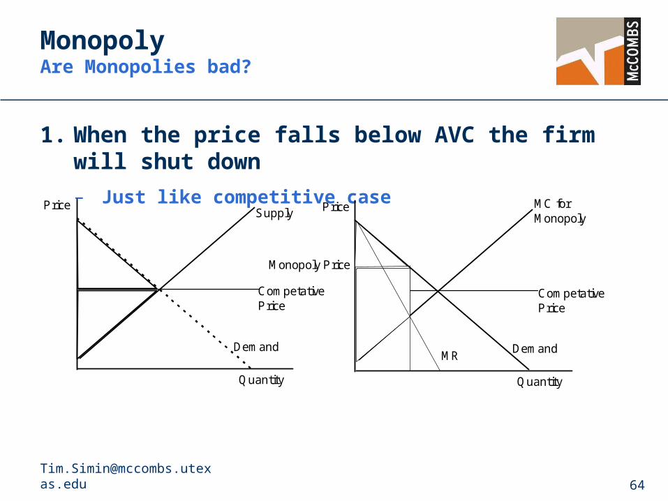
MonopolyAre Monopolies bad?
1. When the price falls below AVC the firm will shut down
– Just like competitive case
CompetativePrice
Demand
Price
Quantity
Supply
CompetativePrice
Demand
Price
Quantity
MC forMonopoly
Monopoly Price
MR
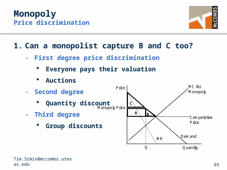
MonopolyPrice discrimination
1. Can a monopolist capture B and C too?
– First degree price discrimination
Everyone pays their valuation
Auctions
– Second degree
Quantity discount
– Third degree
Group discounts
CompetativePrice
Demand
Price
Quantity
MC forMonopoly
Monopoly Price
MR
C
A
Q
B
![Home page []ISKRA-AS (1.0.0. Tuzla Simin Han, Put Tanoviéi do br. 9. 75000 Tuzla Naziv i sjedište ponudaëa ISKRA-AS (1.0.0. Tuzla Simin Han, Put Tanoviéi do br. 9. 75000 Tuzla](https://img.pdfslide.us/doc/110x75/60c4489a887af66e943f5890/home-page-iskra-as-100-tuzla-simin-han-put-tanovii-do-br-9-75000-tuzla.jpg)