CHAPTER I

INTRODUCTION

1.1BACKGROUNDUnlike other classes of real estate, hotels typically contain hundreds (in some

cases over one thousand) of employees. Properties are reliant on the quality of

management, the brand, the employees and other factors. The success of a hotel

investment is heavily influenced by multiple parties, each of which may have competing

and/or complimentary interests in the underlying property. In addition to the traditional

interests of owner/sponsors, third party equity investors, and lenders, additional

complexity is derived from the interests of the property manager and/or brand. These

complexities can result in competing economic and operating influences that may not be

common to other forms of real estate investment.

1.1.1 HOTEL SUPPLY ANALYSIS

A. Huge Area Market Analysis:

Economic and Demographic Analysis:

• Population

• Retail Sales

• Work Force Characteristics

• Major Businesses and Industry

• Office Space

• Highway Traffic

• Airport Statistics

Size and Neighborhood Analysis:

• Size, Terrain and Physical Suitability

• Zoning and other applicable regulations

• Utilities and other services availability

• Access

• Visibility

• Proximity to demand generators

• Excess Land

Subject Hotel Improvement Analysis:

• Number of Rooms

• Food and Beverage Facilities

• Meeting Facilities

• Recreational and Retail Amenities

• Physical Condition

• Effective Age

• Functionality

B. Lodging Supply Analysis

Lodging Classifications

Hotel Type Categories:

• Commercial

• Convention

• Resort

• Suite

• Extended Stay

• Conference Center

• Casino

• Bed & Breakfast

Hotel Location Categories

• Airport

• Highway

• Downtown

• Suburban

• Convention Center

• Resort

Hotel Chain Scale Categories

• Luxury: Ritz Carlton, Four Seasons, Mandarin Oriental, St. Regis, Grand Hyatt

• Upscale:Hilton Garden Inn, Courtyard Marriott, Crown Plaza, Four Points,

Holiday Inn, Quality Inn, Ramada, Best Western, Red Lion

• Midscale without Food & Beverage: Country Inn & Suites, Hampton Inn, Holiday

Inn Express, Comfort Inn, La Quinta, Wingate

• Economy: Days Inn, Extended Stay America, Microtel, Red Roof, Super 8, Value

Place, Rodeway Inn

Lodging Classifications

Hotels.com– Star System

• Five Star - (Deluxe): These are hotels that offer only the highest level of

accommodations and services. The hotels are most often located near other

hotels of the same caliber and are usually found near shopping, dining and other

major attractions. Typical National Chains: Hyatt, Marriott.

• Three Star - (First Class): Typically these hotels offer more spacious

accommodations that include well appointed rooms and decorated lobbies. They

are often located near major expressways or business areas, convenient to

shopping and moderate to high priced attractions. Typical National Chains:

Holiday Inn, Hilton.

• Two Star - (Moderate): Typically smaller hotels managed by the proprietor. The

hotel is often 2 - 4 stories high and usually has a more personal atmosphere.

Typical National Chains: Days Inn, LaQuinta Inn.

• One Star - (Moderate): Usually denotes independent and name brand hotel

chains with a reputation for offering consistent quality amenities. The hotel is

usually small to medium-sized and conveniently located to moderately priced

attractions. Typical National Chains: Econolodge, Motel 6.

Evaluation of Competition

• Primary: same transient visitors as subject property

• Secondary: same transient visitors as subject property, but under special

circumstances

1.1.2. HOTEL DEMAND ANALYSIS

A. Characteristics of Travel Demand

• Commercial/Corporate Individual

• Meeting and Convention

• Leisure

• Government

• Contract Crew

B. Demand Generator Build Up Approach

• Definition of Market Area

• Potential Demand Generators

• Demand Interviews and Surveys

C. Lodging Demand Generators:

• Airports

• Amusement parks

• Association headquarters

• Casinos

• Colleges and universities

Companies and businesses

Convenient highway stopping

points Convention centers

• County seats and state capitals

Court houses

• Festival sites

• Historical attractions

• Hospitals

• Military installations

• Museums

• Offices and industrial parks

• National or state parks and

scenic areas Racetracks

• Regional shopping centers

• Resort areas

• Sports stadiums

• Theaters

• Tourist attractions

• World and state fairs

Lodging Activity Build Up Approach

• Current Accommodated Room Night Demand

• Current and Forecasted Latent Demand:

• Unaccommodated Demand – Nature of Demand

• Area Occupancy Level

• Number of Fill Nights

• Alternative Accommodations

• Induced Demand

• Accomodatable Latent Demand

• Usable Latent Demand

• Forecasted Accommodated Room Night Demand

• Total Available Room Nights

• Overall Market wide Occupancy

1.1.3 ANALYSIS OF MARKET SHARE, OCCUPANCY RATE

A. Average Room Rates

Market Penetration Analysis

• Fair Share

• Market Share

• Penetration Index

• Project Occupancy Up To stabilization

Forecasted Monthly Occupancy Analysis

• Peak Season

• Low Season

• Shoulder Season

B. Average Room Rate Analysis

• Competitive Positioning Method

• Bottom Up Method

• Rule of Thumb Method

• Market Segmentation Method

1.1.4 THE PLAZA HOTEL GLODOK

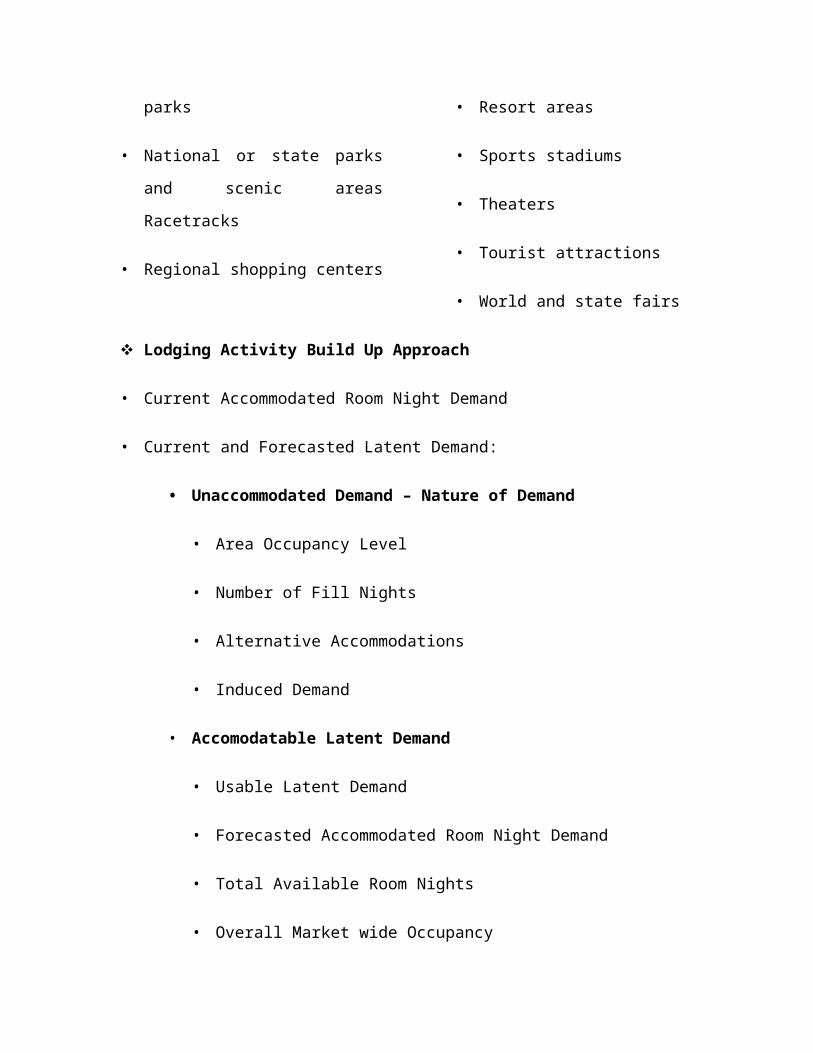
Plaza Hotel Glodok is located on the 3rd floor, in Glodok Plaza shopping center

building and has a capacity of 91 rooms. It is located right in the heart of Glodok.

Glodok are the part of Jakarta’s past. The area is known as the biggest ‘Chinatown’

since the era of Dutch rule in Indonesia. Nowadays, Glodok areas are known as the

center of Jakarta’s largest electronics. Surrounded by a large center such as Lindeteves

(LTC), Pasar Pagi, Glodok Jaya, Orion Plaza, which is as large and famous as Gajah

Mada Plaza and Mangga Dua along the Mangga Besar and Hayam Wuruk street.

Glodok Plaza building is surrounded by several museums and historic buildings as

well as “Kota” train station, which can be reached within minutes from the hotel and

Soekarno-Hatta International Airport which can be reached in less than 45 minutes from

the hotel. The Plaza Hotel Glodok offers simple but clean and comfortable with a warm

and friendly as well as economical prices

A. ROOM

There are 3 types of room in The Plaza Hotel Glodok:

a. Deluxe Room

Room size: 23 m²

Spacious room with KingKoil Duvet bed

Air Conditioner

Sofa and Coffee table

City View

32” LCD TV with International channels

Wi-Fi (in-room Internet Access)

In-room Safe

Walk-in shower (with Normal and Hot temperature)

b. Superior Room

Room size: 20 m²

Spacious room with KingKoil Duvet bed

Air Conditioner

32” LCD TV with International channels

Wi-Fi (in-room Internet Access)

In-room Safe

Walk-in Shower (with normal and hot temperature)

c. Twin Superior Room

Room size: 20 m²

Spacious room with 2 twin KingKoil Duvet beds

Air Conditioner

32” LCD TV with International channels

Wi-Fi (in-room Internet Access)

In-room Safe

Walk-in Shower (with normal and hot temperature)

B. HOTEL FACILITIESThe Plaza Hotel Glodok offers competitive room rate, managed by professional

staffs with facilities, such as:

24-hour front desk service

Wi-Fi (internet access inside and outside the room)

The Plaza Kitchen Restaurant

Spacious rooms with King Koil Duvet bed

32" LCD TV with international channels

Safety deposit box

Walk-in Shower

1.2RESEARCH PROBLEMS

1.3RESEARCH PURPOSEThis research study purpose is to find out what is the main factor that can be the

biggest influence of The Plaza Hotel Glodok’s profit.

1.4SIGNIFICANCES OF STUDYBy looking from the demand and supply of The Plaza Hotel Glodok’s data.

1.5LIMITATIONSAnalysis of demand and supply based on the data of room available and room sold.

CHAPTER II

LITERATURE REVIEW

2.1 DemandOn the demand side of a market, consumers buy products from firms. The main

question concerning the demand side of the market is: How much of a particular product

are consumers willing to buy during a particular period? A consumer who is willing to

buy a particular product is willing to sacrifice enough money to purchase it. The

consumer doesn’t merely have a desire to buy the good, but is willing and able to

sacrifice something to get it. Notice that demand is defined for a particular period, for

example, a day, a month, or a year.

Here is a list of the variables that affect an individual consumer’s decision, which

called as determinants of demand:

• The price of the product

• The consumer’s income

• The price of related goods

• The size and composition of the population

• The consumer’s preferences or tastes and advertising that may influence preferences

• The consumer’s expectations about future prices

Together, these variables determine how much of a particular product an individual

consumer is willing and able to buy, the quantity demanded. The relationship between

the price and quantity demanded is represented graphically by the demand curve

below.

Figure 2.1 Market Demand Curve

Notice that demand curve is negatively sloped, reflecting the law of demand. This law

applies to all consumers.

Market Effects of Changes in Demand:

a. Change in Quantity Demanded

Changes in the price of a good lead to a change in the quantity demanded of that

good. This corresponds to a movement along a given demand curve.

Figure 2.2 Changes in Quantity Demanded

b. Change in Demand

Changes in variables other than the price of a good; such as consumer income,

price of related good, advertising and consumer taste, population and consumer

expectation (demand shifter); lead to a change in demand. This corresponds to a

shift of the entire demand curve.

Figure 2.3 Changes in Demand

Demand Function:

An equation representing the demand curve:

Qxd = f(Px , PY , M, H,)

Where:

Qxd = quantity demand of good X.

Px = price of good X.

PY = price of a related good Y.

M = income.

H = any other variable affecting demand

Demand is linear if Qxd is a linear function of prices, income, and other variables that

influence demand, the following is a linear demand function:

Qxd = α0 + αxPx + αyPy + αMM + αHH

The αs are fixed numbers that the firm’s research department or an economic consultant

typically provides to the manager.

2.2. SupplyOn the supply side of a market, firms sell their products to consumers. Suppose

you ask the manager of a firm, “How much of your product are you willing to produce

and sell?” The answer is likely to be “it depends.” The manager’s decision about how

much to produce depends on many variables, including the following:

• The input prices

• The technology or Government Regulation

• Number of firms

• Substitutes in production

• Producers’ expectations about future prices

• Taxes paid to the government or subsidies (payments from the government to firms to

produce a product)

Together, these variables determine how much of a product firms are willing to produce

and sell, the quantity supplied. The relationship between the price of a good and the

quantity of that good supplied is represented graphically by the supply curve below.

Figure 2.4 Market Supply Curve

The supply curve is positively sloped, reflecting the law of supply, a pattern of behavior

that we observe in producers.

Market Effects of Changes in Supply:

a. Change in Quantity Supplied

Changes in the price of a good lead to a change in the quantity supplied oh that

good. This corresponds to a movement along a given supply.

Figure 2.5 Changes in Quantity Supplied

b. Change in Supply

Changes in variables other than price of a good; such as input price, technology or

government regulation, number of firms, substitutes in production, taxes and

producer expectation (supply shifter); lead to a change in supply. This corresponds

to a shift of the entire supply curve.

Figure 2.6 Changes in Supply

Demand Function:

An equation representing the supply curve:

QxS = f(Px , PR ,W, H,)

Where:

QxS = quantity supplied of good X.

Px = price of good X.

PR = price of a related good

W = price of inputs (e.g., wages)

H = other variable affecting supply

Supply is linear if Qxs is a linear function of the variables that influence supply, the

following is a linear supply function:

Qxs = β0 + βxPx + βRPR + βWW + βHH

The βs are fixed numbers that the firm’s research department or an economic consultant

typically provides to the manager.

2.3. Market EquilibriumA market is an arrangement that brings buyers and sellers together. We bring the

two sides of the market together to show how prices and quantities are determined.

When the quantity of a product demanded equals the quantity supplied at the prevailing

market price, this is called market equilibrium. When a market reaches equilibrium,

there is no pressure to change the price. In Figure 2.7, the equilibrium price is shown by

the intersection of the demand and supply curves. At a certain price, the supply curve

shows that firms will produce number of products, which is exactly the quantity that

consumers are willing to buy at that price.

Figure 2.7 Market Equilibrium

Excess Demand Causes the Price to RiseIf the price is below the equilibrium price, there will be excess demand for the

product. Excess demand (called a shortage) occurs when, at the prevailing market

price, the quantity demanded exceeds the quantity supplied, meaning that consumers

are willing to buy more than producers are willing to sell. In Figure 2.8, at a price of $5,

there is an excess demand equal to 6 goods:

Consumers are willing to buy 12 goods (point c), but producers are willing to sell

only 6 goods (point b). This mismatch between demand and supply will cause the price

of good to rise. Firms will increase the price they charge for their limited supply of

goods, and anxious consumers will pay the higher price to get one of the few goods that

are available. An increase in price eliminates excess demand by changing both the

quantity demanded and quantity supplied. As the price increases, the excess demand

shrinks for two reasons:

• The market moves upward along the demand curve (from point c toward point a),

decreasing the quantity demanded.

• The market moves upward along the supply curve (from point b toward point a),

increasing the quantity supplied.

Because the quantity demanded decreases while the quantity supplied

increases, the gap between the quantity demanded and the quantity supplied narrows.

The price will continue to rise until excess demand is eliminated. In Figure 2.8, at a price

of $7 the quantity supplied equals the quantity demanded, as shown by point a. In some

cases, government creates an excess demand for a good by setting a maximum legal

price that can be charged, called price ceiling. If the government sets a maximum price

that is less than the equilibrium price, the result is a permanent excess demand for the

good.

Figure 2.8 Shortage Condition

Excess Supply Causes the Price to DropWhat happens if the price is above the equilibrium price? Excess supply (called

a surplus) occurs when the quantity supplied exceeds the quantity demanded, meaning

that producers are willing to sell more than consumers are willing to buy. This is shown

by points d and e in Figure 2.9. At a price of $9, the excess supply is 8 goods:

Producers are willing to sell 14 goods (point e), but consumers are willing to buy only 6

goods (point d). This mismatch will cause the price of goods to fall as firms cut the price

to sell them. As the price drops, the excess supply will shrink for two reasons:

• The market moves downward along the demand curve from point d toward point a,

increasing the quantity demanded.

• The market moves downward along the supply curve from point e toward point a,

decreasing the quantity supplied.

Because the quantity demanded increases while the quantity supplied

decreases, the gap between the quantity supplied and the quantity demanded narrows.

The price will continue to drop until excess supply is eliminated. In Figure 2.9, at a price

of $7, the quantity supplied equals the quantity demanded, as shown by point a. The

government sometimes creates an excess supply of a good by setting a minimum legal

price that can be charged, called price floor. If the government sets a minimum price

that is greater than the equilibrium price, the result is a permanent excess supply.

Figure 2.9 Surplus Condition

Now we know that equilibrium is determined in a competitive market and also

government policies such as price ceiling and price floor affect the market. Next, we can

use supply and demand to analyze the impact of changes in market condition on the

competitive equilibrium price and quantity. The study of the movement from one

equilibrium to another is known as comparative static analysis. Throughout this

analysis, no legal restraints, such as price ceiling and price floor, are in affect and that

the price system is free to allocate goods among consumers.

Figure 2.10 shows the change in demand, demand increase, shifting demand curve to

D1 and intersect with supply curve at a new point (red point). In this instance, the market

price rises from P0 to P1 and the equilibrium quantity increases from Q0 to Q1.

Figure 2.10 Effect of change in demand

Figure 2.11 shows the change in supply, supply increase, shifting supply curve to S 1

and intersect with demand curve at a new point (red point). In this instance, the market

price decreases from P0 to P1 and the equilibrium quantity increases from Q0 to Q1.

Figure 2.11 Effect of change in supply

2.4. Elasticity The quantity demanded of a good is affected mainly by:

- changes in the price of a good,

- changes in price of other goods,

- changes in income and,

- changes in other relevant factors.

Elasticity is a measure of just how much the quantity demanded will be affected

by a change in price or income or change in price of related goods. Different elasticities

of demand measures the responsiveness of quantity demanded to changes in variables

which affect demand so:

1. Price elasticity of demand- measures the responsiveness of quantity demanded by

changes in the price of the good

2. Income elasticity of demand – measures the responsiveness of quantity

demanded by changes in consumer incomes.

3. Cross elasticity of demand – measures the responsiveness of quantity demanded

by changes in price of another good

Price elasticity of demand Assume that the price of coke increases by 1 %. If the quantity demanded

consequently falls by 20%, then there is very large drop in quantity demanded in

comparison to the change in price. The price elasticity of coke would be said to be very

high. If quantity demanded fall by 0.01%, then the change in quantity demanded is

relatively insignificant compared to the large change in price and the price elasticity of

coke would be said to be low.

Economists choose to measure responsiveness in term of percentage changes.

So price elasticity of demand which is the degree of responsiveness in changes in

quantity demanded to changes in price is calculated by using the formula:

% Change In Quantity Demanded

% Change In Price

Graphical presentation for price elasticity shown by picture below:

Figure 2.12 Price elasticity

Perfectly inelastic : Quantity demanded does not change at all as P changes, E = 0.

Inelastic : Quantity demanded changes by a smaller percentage than does price , |E| <1

Unitary elasticity : Quantity demanded changes by exactly the same percentage as

does price , |E| = 1

Elastic : Quantity demanded changes by a larger percentage than does price, |E| > 1

Perfectly elastic : Buyers are prepared to purchase all they can obtain at some given

price but none at all at a higher price , E = infinity

Income elasticity of demand The demand for a good will change if there is a change in consumers` income.

Income elasticity of demand is a measure of how much the quantity demanded of a

good responds to a change in consumers’ income. Formula for measuring income

elasticity of demand is

Inferior goods are goods for which an increase in income leads to a decrease in

the demand for that good, or vice versa. It is any goods whose income elasticity of

demand is lower than zero (|Ey| < 0). Normal goods are any goods whose income

elasticity of demand is greater than zero (|Ey| > 0). Normal good are goods for which an

increase (decrease) in income leads to an increase (decrease) in the demand for that

good. Examples of items with a high income elasticity of demand are holidays and

recreational activities, whereas washing up liquids tends to have a low income elasticity

of demand.

Figure 2.12 Income elasticity

Positive Income Elasticity can be divided into 3 categories:

1. Income inelastic : |Ey| < 1 (Dd rises by a smaller proportion as Y)

2. Unit income elasticity: |Ey| = 1 (Dd rises by exactly the same proportion as Y)

3. Income elastic : |Ey| > 1 (Dd rises by a greater proportion than Y)

Cross elasticity of demand The quantity demanded of a particular good varies according to the price of other

goods. A rise in price of a good such as beef would increase the quantity demanded of

a substitute such as chicken; On the other hand a rise in price of a good such as tennis

racket would lead to a fall in quantity demanded of a complement such as tennis ball.

Cross elasticity of demand is a measure of how much the quantity demanded of one

good responds to a change in the price of another good. The formula for calculating the

cross elasticity of demand for good is X:

Two goods, which are substitutes, will have a positive cross elasticity.

Substitutes are goods for which an increase (decrease) in the price of one good leads to

an increase (decrease) in the demand for the other good. It is any goods whose cross

elasticity of demand is greater than zero (|Ex| > 0).

Two goods, which are complements, will have a negative cross elasticity.

Compliments are goods for which an increase (decrease) in the price of one good leads

to an decrease (increase) in the demand for the other good. It is any goods whose cross

elasticity of demand is greater than zero (|Ex| < 0).

The cross elasticity of two goods which have little relationship to each other

would be zero e.g. a rise in the price of cars of 10% is likely to have no effect (0%)

change on the demand for tipp-ex.

2.5 PAST RESEARCHESJack Corgel and Jamie Lane on their research about “Hotel Industry Demand

Curves” extend previous work on understanding hotel demand by focusing on the

demand curve. Specifically, attention is directed toward the slope of the curve indicating

the relationship between average daily rate and the number of rooms sold - the price

elasticity. Price and income elasticity are considerably larger for higher quality hotels, as

indicated by the chain scale in which they operate. Elasticity tends to increase with data

disaggregation. Higher elasticity is generally found for individual chain scales and cities

compared to the nation. The expected direction of the relationship between hotel

demand and each economic variable. For example, as ADRs increase, consumers

purchase fewer hotel rooms, hence the negative sign. As income and employment

increase, consumers have greater abilities to purchase hotel rooms, hence the positive

direction of these relationships.

Aki Hiro Sato (2013) on his research “Detecting Demand Supply: Situations of

Hotel Opportunities: An Empirical Analysis of Japanese Room Opportunities Data”

analyzes the availability of room opportunity types collected from a Japanese hotel

booking site, he characterize demand supply situations of room process at each region

with both room availability and average room rate. The average room rate decreases in

terms of the room rate increase with respect to the room availability in some districts.

This is evidence that the theory of demand and supply is not always satisfied in

Japanese hotel industry.