Embed Size (px)
Citation preview
Manager Characteristics and Capital
Structure: Theory and Evidence
Sanjai Bhagat
Leeds School of Business
University of Colorado, Boulder
Brian Bolton
Whittemore School of Business and Economics
University of New Hampshire
Ajay Subramanian∗
J. Mack Robinson College of Business
Georgia State University
∗Corresponding author. We thank the anonymous referee for several comments and suggestions. AjaySubramanian is very grateful to Steve Hackman for his encouragement, support and comments throughoutthe long gestation period of this research. We also appreciate the comments of Peter DeMarzo, Alex Edmans,Alexander Gorbenko, Dirk Hackbarth, Christopher Hennessy, Kose John, Erwan Morellec, Gustav Sigurds-son, Sanjay Srivastava, Ilya Strebulaev, Toni Whited, Jeffrey Zwiebel and seminar audiences at the secondFoundation for Advanced Research in Financial Economics (FARFE) conference, the 2009 Association ofFinancial Economists (AFE) Meetings (San Francisco, CA), the 2008 Western Finance Association (WFA)
2
Abstract
We investigate the effects of manager characteristics on capital structure in a struc-
tural model. We implement the manager’s optimal contracts through financial secu-
rities that leads to a dynamic capital structure, which reflects the effects of taxes,
bankruptcy costs and manager-shareholder agency conflicts. Long-term debt declines
with the manager’s ability, inside equity stake and the firm’s long-term risk, but in-
creases with its short-term risk. Short-term debt declines with the manager’s ability,
increases with her equity ownership, and declines with short-term risk. We show sup-
port for these implications in our empirical analysis.
JEL Classification Codes: G32, D92, D86
Meetings (Waikoloa, HI), the 2008 Financial Intermediation Research Society (FIRS) Meetings (Anchorage,AK), and the 2008 Financial Management Association (Europe) (FMA) Meetings (Prague, Czech Republic)for valuable comments. The usual disclaimers apply.
1
I Introduction
We theoretically and empirically analyze the effects of managerial incentives and manager-
specific characteristics on capital structure. We develop a dynamic structural model that
incorporates the effects of taxes, bankruptcy costs, as well as agency conflicts between an
undiversified manager and well-diversified outside investors. The manager has discretion
in financing and effort, and receives dynamic incentives through explicit contracts with
shareholders. We implement the manager’s contracts through financial securities, which
leads to a dynamic capital structure for the firm consisting of inside equity, outside equity,
long-term debt, and short-term debt (or a cash reserve).
We derive novel, testable predictions that link manager and firm characteristics to long-
term debt. Long-term debt declines with the manager’s ability, her inside equity stake, and
the firm’s long-term risk, but increases with its short-term risk. Our implementation of the
manager’s contracts also generates additional predictions for the effects of manager and firm
characteristics on short-term debt and total debt. Short-term and total debt decline with the
manager’s ability, increase with her inside equity stake, decline with the firm’s short-term
risk, but vary non-monotonically with its long-term risk. With the exception of the predicted
relation between short-term debt and inside equity, we show significant support for all the
above implications in our empirical analysis.
In our infinite horizon, continuous-time framework, the manager of a privately held firm
obtains financing for a positive NPV project from public debt and equity markets. The
manager has an initial ownership stake and receives a proportion of the net payoff from
external financing (the total proceeds from financing net of the required capital investment).
The firm’s capital structure initially consists of equity, infinite maturity and non-callable
long-term debt, and non-discretionary short-term debt that is associated with the firm’s
working capital requirements such as the financing of inventories, accounts receivable, and
employee wages. In our subsequent implementation of the manager’s contracts, the manager
holds an inside equity stake and her cash compensation is implemented through a cash
reserve that offsets the firm’s short-term debt. In our implementation, therefore, the firm’s
2
capital structure consists of inside and outside equity, long-term debt, and short-term debt
associated with working capital and the manager’s cash compensation.
The total earnings (before interest, taxes, and the manager’s compensation) evolve as
a log-normal process and consist of two components: a component that increases with the
manager’s ability and effort, and a component that represents the earnings from existing
assets that are unaffected by the manager’s human capital. The firm’s earnings are affected
by two sources of uncertainty. First, the earnings generated by the manager in each period
are risky; their standard deviation is the firm’s short-term risk. Second, the firm’s assets
evolve stochastically; their standard deviation is the firm’s long-term risk.
Outside investors are risk-neutral and competitive as in Chapters 3 and 4 of Tirole (2006),
while the undiversified manager has quadratic (mean-variance) preferences. We consider
an incomplete contracting environment in which the manager receives dynamic incentives
through a sequence of explicit contracts contingent on the firm’s earnings. The contracts
must guarantee that the expected payout flow to the firm net of the manager’s compensation
is at least as great as the payout flow from existing assets.
As in Leland (1998), debt is serviced entirely as long as the firm is solvent by the addi-
tional issuance of equity if necessary. Bankruptcy occurs endogenously when the equity value
falls to zero. The firm is subsequently controlled by debt-holders as an all-equity firm. The
firm’s future earnings after bankruptcy are lowered by bankruptcy costs that are external
to the manager-firm relationship. The manager continues to operate the firm, and contracts
with debt-holders, who are the firm’s new shareholders. The manager also incurs personal
bankruptcy costs because her compensation is tied to the firm’s earnings.
We characterize the equilibrium in which the firm’s capital structure and the manager’s
contracts are endogenously determined. Because the manager has an initial ownership stake,
she receives a portion of the net payoff—the total proceeds net of the required capital
investment—from external financing. The manager chooses the firm’s capital structure to
maximize the total expected utility she derives from her initial payoff from leveraging the
firm and her stream of future contractual compensation payments.
The manager’s compensation in each period is affine in the firm’s earnings. We imple-
3
ment the risky component of the manager’s compensation through an inside equity stake in
the firm, and the performance-invariant or “cash” component through a cash reserve that
modifies the firm’s short-term debt. (Cash is effectively negative short-term debt; see De-
Marzo and Fishman (2007).) The different components of the firm’s capital structure play
complementary roles. The firm’s long-term debt primarily reflects the tradeoff between debt
tax shields and bankruptcy costs. The manager’s inside equity stake and the cash reserve
provide optimal incentives to the risk-averse manager.
We first derive a number of results linking manager and firm characteristics to long-term
debt that do not depend on our implementation of the manager’s compensation contracts.
The manager’s long-term debt choice at date zero reflects its effects on her initial payoff
from leveraging the firm, and the expected utility from her future contractual compensation
payments—hereafter, her continuation value. The manager’s initial payoff from leveraging
the firm is proportional to the total proceeds from external financing net of the initial required
investment. Under rational expectations, the proceeds from external financing equal the
market value of the firm’s total after-tax earnings net of the manager’s stake.
The long-term debt choice trades off the positive and negative effects of long-term debt
on the manager’s total expected utility. On the positive side, because debt interest payments
are shielded from corporate taxes, the manager can potentially increase the proceeds from
external financing at date zero (therefore, her initial payoff) by choosing greater long-term
debt. Choosing greater long-term debt, however, increases the expected bankruptcy costs
for the firm and personal bankruptcy costs for the manager, which negatively affect her
continuation value.
We show that long-term debt declines with the manager’s ability, increases with the man-
ager’s risk aversion, and increases with her disutility of effort. To understand the intuition
for these results, we first note that, because capital markets are competitive, the manager
appropriates the surplus she generates due to her human capital (see Aghion and Bolton
(1992), Chapter 3 of Tirole (2006)). Consequently, the manager’s ability and effort affect
her continuation value, but do not affect the proceeds from external financing at date zero
and, therefore, the manager’s initial payoff.
4
An increase in the manager’s ability increases the output the manager generates and her
expected contractual compensation in each period. At the margin, the manager consequently
gives relatively more weight to her continuation value than her initial payoff in choosing the
firm’s long-term debt. Because long-term debt lowers the manager’s continuation value
through the likelihood of bankruptcy, the manager chooses lower long-term debt to lower
the probability of bankruptcy.
An increase in the manager’s risk aversion or disutility of effort increases the costs of
providing incentives to the risk-averse manager so that she exerts lower effort in equilib-
rium. The output she generates in each period and her expected compensation decline. The
manager therefore attaches relatively more weight to her initial payoff from leveraging the
firm than her continuation value. She chooses greater long-term debt to exploit the positive
effects of ex post debt tax shields on the surplus she generates from external financing and,
therefore, her initial payoff.
The negative effect of manager ability, and the positive effect of risk aversion, on long-
term debt are surprising predictions of our theory. Casual intuition would seem to suggest
that manager ability should positively affect long-term debt because it increases the firm’s
earnings in each period, while risk aversion should negatively affect long-term debt because
earnings decline (due to costs of risk-sharing) and the adverse impact of the possibility of
bankruptcy on the manager’s expected utility increases. As discussed above, our results and
the intuition underlying them show that this casual intuition is incorrect.
The firm’s short-term and long-term risks have differing effects on long-term debt. Long-
term debt declines with long-term risk, but increases with short-term risk. Long-term and
short-term risk have differing effects on long-term debt because the short-term risk affects
the manager’s incentive compensation in each period, while the long-term risk has long-
term effects by influencing the manager’s valuation of her future payoffs. The presence of
managerial discretion plays a central role in generating the differing effects of long-term and
short-term risks on debt structure.a
aIn a different framework, Gorbenko and Strebulaev (2010) also show that permanent and temporary
components of a firm’s risk have differing effects on financial policies.
5
Next, we conduct a quantitative investigation of the effects of manager and firm charac-
teristics on capital structure. To obtain a reasonable set of baseline parameter values, we
calibrate the model to the data we use for our subsequent empirical analysis. In particu-
lar, we indirectly infer the manager-specific parameters—ability, risk aversion, discount rate,
and disutility of effort—by matching the predicted values of key relevant statistics to their
average values in the data.
Consistent with our analytical results, long-term debt declines with the manager’s ability,
increases with her risk aversion, increases with her disutility of effort, declines with the firm’s
long-term risk, and increases with its short-term risk. Our numerical analysis shows that
the firm’s short-term debt declines with the manager’s ability, risk aversion and disutility of
effort as well as with the firm’s short-term risk. Because the manager’s ability represents her
non-discretionary contribution to output in each period, an increase in the manager’s ability
increases the performance-invariant or “cash” component of the manager’s compensation
in each period. The value of the firm’s cash reserve (short-term debt), therefore, increases
(decreases).b
An increase in the manager’s risk aversion, disutility of effort, or the firm’s short-term
risk increases the cost of providing incentives to the risk-averse manager. In equilibrium,
the manager’s inside equity stake declines, and she receives a greater portion of her com-
pensation in “cash” rather than risky “equity”. Consequently, the value of the firm’s cash
reserve (short-term debt) again increases (decreases). Recall that the firm’s short-term debt
is determined by its working capital requirements and the manager’s cash compensation.
Manager-specific characteristics affect the firm’s short-term debt through their effects on the
manager’s cash compensation.
Our main testable implications are robust to an extension of the model that accommo-
dates the scenario in which the manager continues to service debt even after the equity value
falls to zero (the firm effectively becomes privately held). The manager declares bankruptcy
when it is no longer optimal for her to continue servicing debt. We also explore the robust-
ness of our implications to another extension of the model that allows for variations in the
bRecall that cash is negative risk-free short-term debt.
6
allocation of bargaining power between insiders and outsiders. The main predictions of the
theory hold as long as shareholders’ bargaining power vis-a-vis the manager is below a (high)
threshold.
We empirically investigate the testable implications of the theory that link manager and
firm characteristics to long-term and short-term debt. For robustness, we use five empirical
proxies for managerial ability. The first three proxies—CEO cash compensation, the ratio of
CEO cash compensation to assets, and the industry-adjusted return on assets of the firm—
are directly derived from the theory. The last two proxies—CEO tenure and the ratio of CEO
tenure to age—are indirect proxies of CEO ability. We show that long-term and short-term
debt decline with all our ability proxies as predicted by the theory.
The theory predicts that long-term debt increases with the manager’s risk aversion and
disutility of effort, while short-term debt declines. As discussed earlier, the manager’s inside
equity stake declines with her risk aversion and disutility of effort, which reflects the greater
costs of providing incentives to the risk-averse manager. The theory, therefore, predicts a
negative relation between long-term debt and the manager’s inside equity ownership, and a
positive relation between short-term debt and inside equity ownership. Consistent with the
theory, long-term debt declines with the manager’s inside equity ownership. The relation
between short-term debt and inside equity ownership is, however, negative and marginally
significant.
We also empirically examine the predicted effects of long-term and short-term risk on
debt structure. Consistent with the theory, our primary proxies for a firm’s long-term and
short-term risk are the asset volatility and the standard deviation of the return on assets,
respectively. As predicted by the theory, we show that long-term debt decreases with long-
term risk and increases with short-term risk, while short-term debt decreases with short-term
risk.
We carry out an instrumental variables analysis to correct for potential econometric issues
created by the endogenous determination of manager ownership and debt structure. With
the exception of the relation between short-term debt and manager ownership, our results
continue to show significant support for the testable implications of the theory even after
7
controlling for endogeneity. To partially address Strebulaev’s (2007) critique that traditional
leverage regressions could be misspecified in a dynamic context, we show support for our
hypotheses in additional tests that examine the incremental financing decisions of firms.
II Related Literature
The tradeoff theory of capital structure argues that capital structure is determined by the
tradeoff between the benefits of debt tax shields and the costs of financial distress. A number
of studies examine the quantitative effects of the tradeoff between taxes and financial distress
costs in dynamic, structural models in which managers are assumed to behave in the interests
of shareholders (for example, Fischer et al (1989), Leland and Toft (1996), Goldstein et al.
(2001), Hennessy and Whited (2005), Strebulaev (2007)).
Because they do not incorporate managerial discretion, manager characteristics have no
effect on capital structure in these models. We contribute to this literature by analyzing
the effects of managerial discretion in a dynamic model that also incorporates taxes and
bankruptcy costs. Apart from reconciling growing evidence on the effects of manager char-
acteristics on financing decisions (Berger et al. (1997), this study), our analysis also sheds
light on the relative importance of taxes, bankruptcy costs, and manager-shareholder agency
conflicts in the determination of capital structure.
The agency theory of capital structure is based on the premise that agency conflicts
between managers and outside investors are a key determinant of capital structure (see My-
ers (2001) for a survey). DeMarzo and Sannikov (2006) and DeMarzo and Fishman (2007)
investigate the effects of agency conflicts on capital structure in dynamic frameworks with
risk-neutral agents and complete contracting.c We complement these studies in several key
respects. First, we incorporate taxes in our framework, which have a first order effect on
capital structure as shown by recent studies (for example, Hennessy and Whited (2005), Stre-
cIn these studies, the current shareholders of the levered firm are committed to a contract signed with
the shareholders of the original un-levered firm. They also consider the impact of ex post Pareto-improving
renegotiations with respect to the contract signed with the original shareholders.
8
bulaev (2007)). Our study, therefore, integrates the perspectives of “tradeoff” and “agency”
models that capital structure reflects the effects of external imperfections such as taxes and
bankruptcy costs as well as internal agency conflicts among firms’ stake-holders. Second,
we derive novel implications for the effects of manager-specific characteristics such as ability
and risk aversion on capital structure. Third, we examine the effects of managerial discretion
in an environment in which contracts are incomplete.
Berk et al. (2006) analyze the effects of managerial risk aversion on capital structure
in a framework with one-sided commitment. We complement their study by developing a
framework with moral hazard (effort provision), incentive compensation, and risky long-term
debt. We implement the manager’s contract through financial securities, which leads to a
dynamic capital structure and implications for the effects of manager and firm characteristics
on long-term debt and short-term debt. Subramanian (2008) develops a continuous-time
agency model to show how a risk-averse manager’s discretion in dynamic financing, effort
and project choices affects capital structure. He (2011) studies the effects of manager-
shareholder agency conflicts on capital structure and finds that the effects of debt overhang
on managerial incentives lowers the optimal leverage.
III The Model
The manager of an all-equity firm obtains financing for a capital investment I > 0 in a pos-
itive NPV project from public debt and equity markets. (The “manager” should be viewed
as a proxy for the firm’s “insiders.”) The manager has an ownership stake ginitial ∈ (0, 1)
in the initial all-equity firm. The total earnings before interest, taxes and the manager’s
compensation (EBITM) are distributed among all the firm’s claimants: the manager, share-
holders, debt-holders, and the government (through taxes). We ignore personal taxes for
simplicity, and assume that the corporate tax rate is a constant τ ∈ (0, 1). Security issuance
costs are negligible and the risk-free interest rate, r, is constant and the same for all market
participants. All agents are fully rational.
9
A The Firm’s Total EBITM Flow
The model is set in continuous time with a time horizon [0,∞). For expositional convenience,
we refer to the interval [t, t + dt] as a “period,” which represents a time period such as one
quarter in the real world. In any period [t, t + dt] ; t ∈ [0,∞), the firm’s existing assets
generate a total EBITM flow P (t)dt without any actions by the manager. The manager
affects the total EBITM flow over time through her ability and unobservable effort. In any
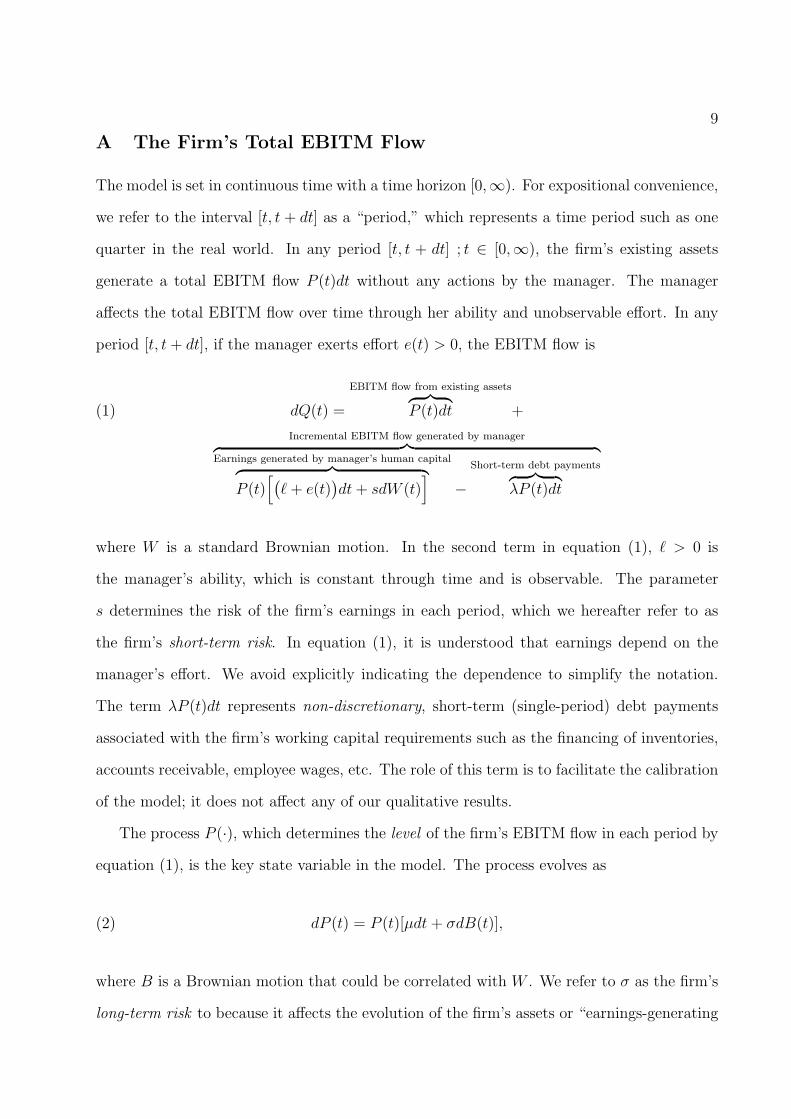
period [t, t+ dt], if the manager exerts effort e(t) > 0, the EBITM flow is
dQ(t) =
EBITM flow from existing assets︷ ︸︸ ︷P (t)dt +(1)
Incremental EBITM flow generated by manager︷ ︸︸ ︷Earnings generated by manager’s human capital︷ ︸︸ ︷
P (t)[(ℓ+ e(t)
)dt+ sdW (t)
]−
Short-term debt payments︷ ︸︸ ︷λP (t)dt
where W is a standard Brownian motion. In the second term in equation (1), ℓ > 0 is
the manager’s ability, which is constant through time and is observable. The parameter
s determines the risk of the firm’s earnings in each period, which we hereafter refer to as
the firm’s short-term risk. In equation (1), it is understood that earnings depend on the
manager’s effort. We avoid explicitly indicating the dependence to simplify the notation.
The term λP (t)dt represents non-discretionary, short-term (single-period) debt payments
associated with the firm’s working capital requirements such as the financing of inventories,
accounts receivable, employee wages, etc. The role of this term is to facilitate the calibration
of the model; it does not affect any of our qualitative results.
The process P (·), which determines the level of the firm’s EBITM flow in each period by
equation (1), is the key state variable in the model. The process evolves as
(2) dP (t) = P (t)[µdt+ σdB(t)],
where B is a Brownian motion that could be correlated with W . We refer to σ as the firm’s
long-term risk to because it affects the evolution of the firm’s assets or “earnings-generating
10
capacity” over time. The project parameters s, µ, σ, which determine the earnings flows over
time, are common knowledge. The information generated by the EBITM process and the
process P (·) is {Ft}.
B The Debt Structure
All long-term debt issued at date zero has infinite maturity, is non-callable, and is completely
amortized so that long-term debt-holders are entitled to a coupon payment θ per unit time
(hereafter, the coupon). The coupon, θ, which determines the firm’s long-term debt structure,
is later determined endogenously. For now, the firm’s capital structure consists of equity,
long-term debt and the short-term debt financing of the firm’s working capital requirements.
In Section V, we implement the manager’s optimal contract through an inside equity stake
and a cash reserve that offsets the firm’s short-term debt. While we could have incorporated
the term λP (t)dt in equation (1) into the earnings generated by the manager’s human capital,
we indicate it separately to clarify the roles of the different components of short-term debt in
the implemented model. We hereafter refer to the firm’s long-term debt-holders as, simply,
its debt-holders.
C The Objectives of Outside Investors and the Manager
Outside investors are risk-neutral, while the manager is risk-averse. If the manager’s payoff
in period [t, t+ dt] is dc(t) and her effort level is e(t), her total expected utility is
(3) Φ(c, e) = E
[∫ ∞
0
exp(−βt)
(U(dc(t))− 1
2κe(t)2dt
)].
In the above, β > 0 is the manager’s subjective discount rate (or “degree of myopia”) and
12κe(t)2dt (κ > 0 is a constant) is the manager’s disutility of effort in period [t, t + dt]. All
our analytical results hold if β = r. We allow for β to differ from the risk-free rate r for
greater generality and to facilitate the calibration of the model. Our calibration exercise in
Section VIA leads to a calibrated value of the manager’s discount rate β that differs from
the risk-free rate. This observation, and the significant level of risk aversion of the manager
11
reflect the fact that the average manager is significantly undiversified. For tractability, we
assume that the manager has quadratic (mean-variance) preferences, that is, the manager’s
utility function U(.) is
(4) U(x) = x− 1
2γx2,
where γ is the manager’s constant risk aversion.
D Contracting
The manager receives dynamic incentives through contracts that could be explicitly contin-
gent on the EBITM flow process, dQ(.). We consider an incomplete contracting environment
in which only single-period contracts are enforceable. As in Chapter 3 of Tirole (2006), the
manager offers a contract to the firm’s competitive shareholders in each period. In our
subsequent implementation of the manager’s contracts in Section V, this is equivalent to
the manager dynamically issuing (or buying back) financial securities in competitive capital
markets. In our implementation, the manager also holds an inside equity stake in the firm.
Anticipating this implementation, we assume that the manager receives her contractually
specified payoff from the total earnings net of corporate taxes. The remaining earnings
are distributed among long-term debt-holders (hereafter referred to as debt-holders) and

12
shareholders.d
As in Leland (1998), debt payments are serviced entirely as long as the firm is solvent.
In financial distress, debt payments are serviced through the additional issuance of equity.
Bankruptcy occurs endogenously when the equity value falls to zero. The absolute priority
of debt is enforced at bankruptcy and the firm is subsequently controlled by debt-holders as
an all-equity firm.e Note that, because the manager’s contracts determine the payout flows
to outside equity, they also effectively determine the bankruptcy time. In Appendix B, we
extend the model to allow for the manager to continue servicing debt from the firm’s total
earnings after the equity value falls to zero, which is effectively equivalent to the scenario
in which the firm becomes privately held. The manager declares bankruptcy when it is no
longer optimal for her to service debt. The implications of the extended model do not differ
from those of the simpler model presented here in which bankruptcy occurs when the equity
value falls to zero.
For simplicity and concreteness, we assume that the manager continues to operate the
firm after bankruptcy and contracts with the new shareholders of the firm; the debt-holders.f
dThis reflects the perspective that the manager is a shareholder so that her compensation is paid out after
corporate taxes. We can easily modify the model to assume that executive compensation is deductible in
the computation of corporate taxes without altering any of our implications. In reality, the tax treatment of
CEO compensation is rather complex. According to Section 162(m) of the Internal Revenue Code, executive
compensation is tax deductible, but only up to a limit of $1 million. Certain types of incentive compensation
such as bonus compensation and qualified stock options are tax deductible, but stock grants, option grants
below market value, and downside protection for an executive in the event of a decline in the stock price
are not. Moreover, the assessed taxes also vary depending on underlying vesting periods. The situation is
complicated further by the fact that personal taxes also depend on the underlying compensation instruments,
exercise times, etc. The differential tax treatment of various components of managerial compensation would
greatly complicate the framework and exposition, but is unlikely to alter the main insights of our study.eWe can extend the model to allow for the firm to be re-levered after bankruptcy. This complicates the
analysis and notation without altering our main implications.fAs we discuss later, the manager also effectively incurs personal costs due to bankruptcy. The man-
ager’s expected future payoffs after bankruptcy in our model could also be re-interpreted as the manager’s
expected payoffs from her “outside options” in a modified model in which the manager leaves the firm af-
ter bankruptcy. As our results only require that the manager incur personal bankruptcy costs, they are
13
The firm bears deadweight costs as a result of bankruptcy that are reflected in a reduction
in future earnings. More precisely, if Tb is the bankruptcy (stopping) time, the state vari-
able P (·), which determines the level of earnings in each period by equation (1) falls by a
proportion ς ∈ (0, 1) at bankruptcy so that
(5) P (Tb) = (1− ς)P (Tb−).
The post-bankruptcy period is otherwise identical to the period during which the firm is
solvent. The effects of the manager’s actions on total earnings are as described in equation
(1) and equation (2). The bankruptcy costs modeled above comprise of direct costs as
well as indirect costs that arise from imperfections in the firm’s product market such as its
relationships with customers and suppliers, which directly affect its asset base or output-
generating capacity. In particular, these costs are due to sources external to the manager-firm
relationship.
We simultaneously describe the contracting before and after bankruptcy because, in
equilibrium, post-bankruptcy actions and earnings, which are rationally anticipated by all
agents, affect pre-bankruptcy actions and earnings. To simplify the notation, we view the
sequence of single-period contracts between the manager and shareholders before bankruptcy
as a single long-term contract that is implemented by this sequence. Similarly, the sequence
of single-period contracts between the manager and debt-holders after bankruptcy are viewed
as a single long-term contract. We further simplify the notation by concatenating the pre
and post-bankruptcy contracts and directly referring to the single combined contract for
the manager. The pre-bankruptcy portion of the contract is between the manager and
shareholders and the post-bankruptcy portion is between the manager and debt-holders.
As in traditional principal-agent models with moral hazard (see Laffont and Martimort
(2002)), it is convenient to augment the definition of the manager’s contract to also include
the manager’s effort. We then require that the manager’s contract be incentive compatible
or implementable with respect to her effort. Formally, a contract Γ ≡ [dcm(·), e(·)] is a
qualitatively unaltered.
14
stochastic process describing the manager’s compensation payments dcm(·) and effort choices
e(·), before and after bankruptcy. The processes dcm(·) and e(.) are Ft-adapted. The
bankruptcy time is an Ft-stopping time Tb (recall that the bankruptcy time is determined
by the contract).
E Payoffs to Shareholders and Debtholders
In our implementation of the manager’s contract in Section V, the manager also holds an in-
side equity stake in the firm. Anticipating this implementation, we assume that the manager
receives her contractually specified payoff from the total earnings net of corporate taxes. For
simplicity, we assume that there is no loss of tax shields on debt interest payments in finan-
cial distress, and taxation is symmetric. For a contract Γ ≡ [dcm(·), e(·)] and bankruptcy
time Tb, it follows from equation (1) that the total after-tax earnings in any period [t, t+ dt]
are
dcf (t) = (1− τ)dQ(t) + τθdt, t < Tb(6)
dcf (t) = (1− τ)dQ(t) t ≥ Tb
The above reflects the fact that corporate taxes are incurred on earnings net of interest
payments on long-term debt.g The payoff to debt-holders during the period is
dcd(t) = θdt, t < Tb(7)
dcd(t) = dcf (t)− dcm(t) t ≥ Tb
As described by the second equation in equation equation (8), debt-holders receive the
residual payout flow after payments to the manager in the post-bankruptcy period. From
equation (7) and equation (8), the payoff to shareholders, which is the total after-tax earnings
gThe interest portion of the short-term debt payments λP (t)dt described in equation (1) are o(dt) so that
the corresponding tax shield vanishes in the continuous-time limit.
15
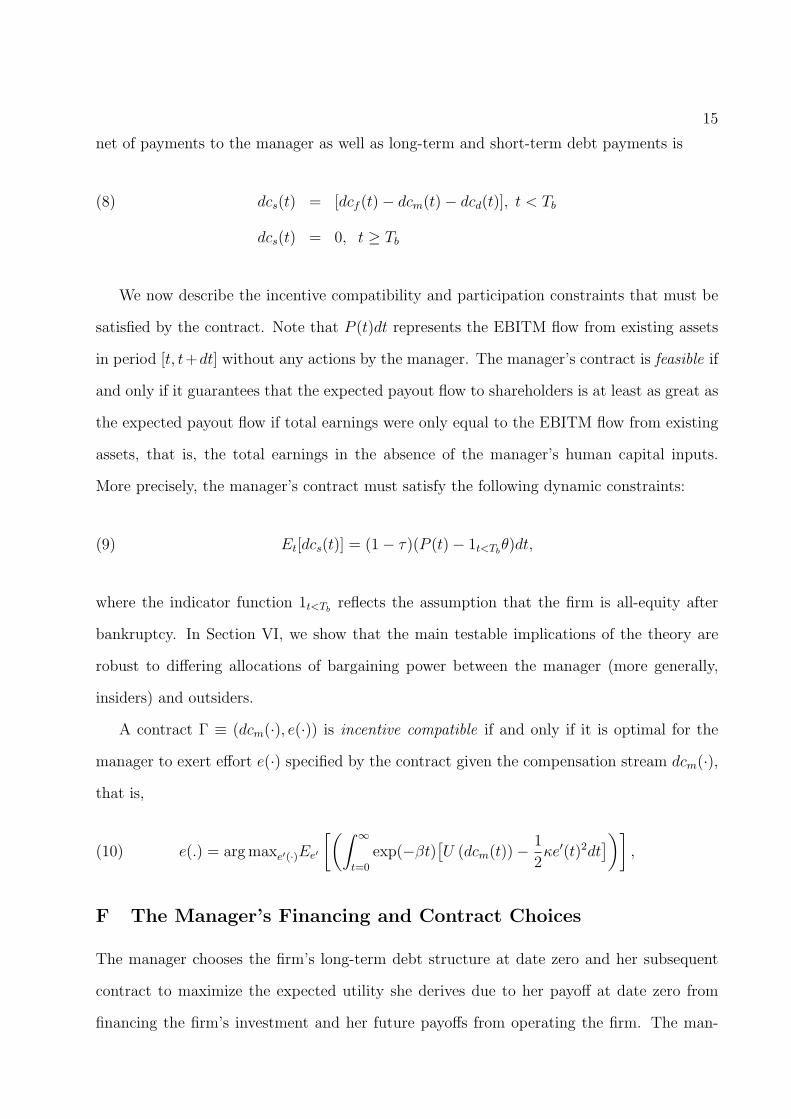
net of payments to the manager as well as long-term and short-term debt payments is
dcs(t) = [dcf (t)− dcm(t)− dcd(t)], t < Tb(8)
dcs(t) = 0, t ≥ Tb
We now describe the incentive compatibility and participation constraints that must be
satisfied by the contract. Note that P (t)dt represents the EBITM flow from existing assets
in period [t, t+dt] without any actions by the manager. The manager’s contract is feasible if
and only if it guarantees that the expected payout flow to shareholders is at least as great as
the expected payout flow if total earnings were only equal to the EBITM flow from existing
assets, that is, the total earnings in the absence of the manager’s human capital inputs.
More precisely, the manager’s contract must satisfy the following dynamic constraints:
(9) Et[dcs(t)] = (1− τ)(P (t)− 1t<Tbθ)dt,
where the indicator function 1t<Tbreflects the assumption that the firm is all-equity after
bankruptcy. In Section VI, we show that the main testable implications of the theory are
robust to differing allocations of bargaining power between the manager (more generally,
insiders) and outsiders.
A contract Γ ≡ (dcm(·), e(·)) is incentive compatible if and only if it is optimal for the
manager to exert effort e(·) specified by the contract given the compensation stream dcm(·),
that is,
(10) e(.) = argmaxe′(·)Ee′
[(∫ ∞
t=0
exp(−βt)[U (dcm(t))−
1
2κe′(t)2dt
])],
F The Manager’s Financing and Contract Choices
The manager chooses the firm’s long-term debt structure at date zero and her subsequent
contract to maximize the expected utility she derives due to her payoff at date zero from
financing the firm’s investment and her future payoffs from operating the firm. The man-
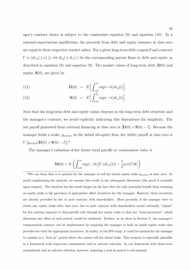
16
ager’s contract choice is subject to the constraints equation (9) and equation (10). In a
rational expectations equilibrium, the proceeds from debt and equity issuance at date zero
are equal to their respective market values. For a given long-term debt coupon θ and contract
Γ ≡ (dcm(.), e(.)), let dcd(·), dcs(·) be the corresponding payout flows to debt and equity as
described in equation (8) and equation (9). The market values of long-term debt, D(0) and
equity, S(0), are given by
D(0) = E[ ∫ ∞
t=0
exp(−rt)dcd(t)],(11)
S(0) = E[ ∫ Tb
t=0
exp(−rt)dcs(t)].(12)
Note that the long-term debt and equity values depend on the long-term debt structure and
the manager’s contract; we avoid explicitly indicating this dependence for simplicity. The
net payoff generated from external financing at date zero is [D(0) + S(0)− I]. Because the
manager holds a stake, ginitial, in the initial all-equity firm, her utility payoff at date zero is
U [ginitial(D(0) + S(0)− I)].h
The manager’s valuation of her future total payoffs or continuation value is
M(0) = E
(∫ ∞
t=0
exp(−βt)[U (dcm(t))−
1
2κe(t)2dt
])hWe can show that it is optimal for the manager to sell her initial equity stake ginitial at date zero. To
avoid complicating the analysis, we assume this result in the subsequent discussion (the proof is available
upon request). The intuition for the result hinges on the fact that the only potential benefit from retaining
an equity stake is the provision of appropriate effort incentives for the manager. However, these incentives
are already provided by her ex post contract with shareholders. More precisely, if the manager were to
retain any equity stake after date zero, her ex post contract with shareholders would rationally “adjust”
for her existing exposure to firm-specific risk through her equity stake so that her “total incentives”, which
determine her effort in each period, would be unaltered. Further, as we show in Section V, the manager’s
compensation contract can be implemented by requiring the manager to hold an inside equity stake that
provides her with the appropriate incentives. In reality, at the IPO stage, it could be optimal for the manager
to commit to a “lock in” period where she cannot sell her initial stake. This scenario is especially plausible
in a framework with long-term commitment and/or adverse selection. In our framework with short-term
commitment and no adverse selection, however, imposing a lock-in period is sub-optimal.
17
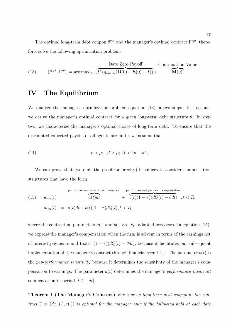
The optimal long-term debt coupon θopt and the manager’s optimal contract Γopt, there-
fore, solve the following optimization problem:
(13) (θopt,Γopt) = argmax(θ,Γ)
Date Zero Payoff︷ ︸︸ ︷U (ginitial(D(0) + S(0)− I))+
Continuation Value︷ ︸︸ ︷M(0). .
IV The Equilibrium
We analyze the manager’s optimization problem equation (13) in two steps. In step one,
we derive the manager’s optimal contract for a given long-term debt structure θ. In step
two, we characterize the manager’s optimal choice of long-term debt. To ensure that the
discounted expected payoffs of all agents are finite, we assume that
(14) r > µ; β > µ; β > 2µ+ σ2,
We can prove that (we omit the proof for brevity) it suffices to consider compensation
structures that have the form
dcm(t) =
performance-invariant compensation︷ ︸︸ ︷a(t)dt +
performance-dependent compensation︷ ︸︸ ︷b(t)(1− τ)(dQ(t)− θdt) , t < Tb(15)
dcm(t) = a(t)dt+ b(t)(1− τ)dQ(t), t > Tb
where the contractual parameters a(.) and b(.) are Ft−adapted processes. In equation (15),
we express the manager’s compensation when the firm is solvent in terms of the earnings net
of interest payments and taxes, (1 − τ)(dQ(t) − θdt), because it facilitates our subsequent
implementation of the manager’s contract through financial securities. The parameter b(t) is
the pay-performance sensitivity because it determines the sensitivity of the manager’s com-
pensation to earnings. The parameter a(t) determines the manager’s performance-invariant
compensation in period [t, t+ dt].
Theorem 1 (The Manager’s Contract) For a given long-term debt coupon θ, the con-
tract Γ ≡ (dcm(·), e(·)) is optimal for the manager only if the following hold at each date
18
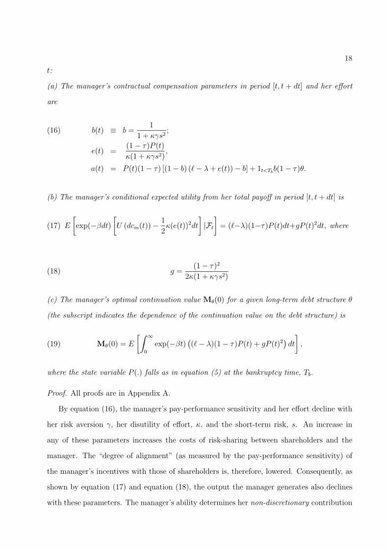
t:
(a) The manager’s contractual compensation parameters in period [t, t + dt] and her effort
are
b(t) ≡ b =1
1 + κγs2;(16)
e(t) =(1− τ)P (t)
κ(1 + κγs2),
a(t) = P (t)(1− τ) [(1− b) (ℓ− λ+ e(t))− b] + 1t<Tbb(1− τ)θ.
(b) The manager’s conditional expected utility from her total payoff in period [t, t+ dt] is
(17) E
[exp(−βdt)
[U (dcm(t))−
1
2κ(e(t))2dt
]|Ft
]= (ℓ−λ)(1−τ)P (t)dt+gP (t)2dt, where
(18) g =(1− τ)2
2κ(1 + κγs2)
(c) The manager’s optimal continuation value Mθ(0) for a given long-term debt structure θ
(the subscript indicates the dependence of the continuation value on the debt structure) is
(19) Mθ(0) = E
[∫ ∞
0
exp(−βt)((ℓ− λ)(1− τ)P (t) + gP (t)2
)dt
],
where the state variable P (.) falls as in equation (5) at the bankruptcy time, Tb.
Proof. All proofs are in Appendix A.
By equation (16), the manager’s pay-performance sensitivity and her effort decline with
her risk aversion γ, her disutility of effort, κ, and the short-term risk, s. An increase in
any of these parameters increases the costs of risk-sharing between shareholders and the
manager. The “degree of alignment” (as measured by the pay-performance sensitivity) of
the manager’s incentives with those of shareholders is, therefore, lowered. Consequently, as
shown by equation (17) and equation (18), the output the manager generates also declines
with these parameters. The manager’s ability determines her non-discretionary contribution
19
to output (see equation 1). As a result, the manager’s ability only affects the performance-
invariant component of her compensation.
In equation (19), the manager’s continuation value is affected by the long-term debt
structure through its effect on the bankruptcy time Tb. Since the manager’s expected payoff
in each period depends on the state variable P (.)̇ as shown by equation (17), she incurs
personal costs after bankruptcy because the state variable P (.)̇ falls as in equation (5) at the
bankruptcy time, Tb.
In the extended model presented in Appendix B, where the manager continues to service
debt after the equity value falls to zero, the manager’s contractual parameters when the
firm becomes privately held differ from the contractual parameters described in Theorem 1.
In particular, her effort as a proportion of the state variable P (t) and her pay-performance
sensitivity are higher (see Proposition 1 in Appendix B).
We now determine the market values of long-term debt, equity and the bankruptcy time.
As in Leland (1998), bankruptcy occurs when the state variable P (.) falls to an endogenous
trigger pb(θ).
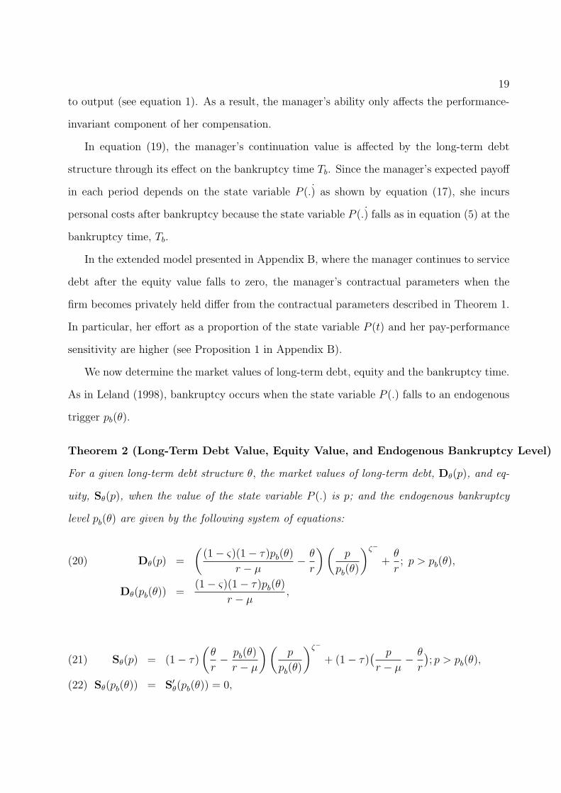
Theorem 2 (Long-Term Debt Value, Equity Value, and Endogenous Bankruptcy Level)
For a given long-term debt structure θ, the market values of long-term debt, Dθ(p), and eq-
uity, Sθ(p), when the value of the state variable P (.) is p; and the endogenous bankruptcy
level pb(θ) are given by the following system of equations:
Dθ(p) =
((1− ς)(1− τ)pb(θ)
r − µ− θ
r
)(p
pb(θ)
)ζ−
+θ
r; p > pb(θ),(20)
Dθ(pb(θ)) =(1− ς)(1− τ)pb(θ)
r − µ,
Sθ(p) = (1− τ)
(θ
r− pb(θ)
r − µ
)(p
pb(θ)
)ζ−
+ (1− τ)( p
r − µ− θ
r
); p > pb(θ),(21)
Sθ(pb(θ)) = S′θ(pb(θ)) = 0,(22)
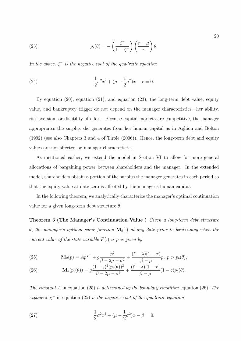
20
(23) pb(θ) = −(
ζ−
1− ζ−
)(r − µ
r
)θ.
In the above, ζ− is the negative root of the quadratic equation
(24)1
2σ2x2 + (µ− 1
2σ2)x− r = 0.
By equation (20), equation (21), and equation (23), the long-term debt value, equity
value, and bankruptcy trigger do not depend on the manager characteristics—her ability,
risk aversion, or disutility of effort. Because capital markets are competitive, the manager
appropriates the surplus she generates from her human capital as in Aghion and Bolton
(1992) (see also Chapters 3 and 4 of Tirole (2006)). Hence, the long-term debt and equity
values are not affected by manager characteristics.
As mentioned earlier, we extend the model in Section VI to allow for more general
allocations of bargaining power between shareholders and the manager. In the extended
model, shareholders obtain a portion of the surplus the manager generates in each period so
that the equity value at date zero is affected by the manager’s human capital.
In the following theorem, we analytically characterize the manager’s optimal continuation
value for a given long-term debt structure θ.
Theorem 3 (The Manager’s Continuation Value ) Given a long-term debt structure
θ, the manager’s optimal value function Mθ(.) at any date prior to bankruptcy when the
current value of the state variable P (.) is p is given by
Mθ(p) = Apχ−+ g
p2
β − 2µ− σ2+
(ℓ− λ)(1− τ)
β − µp; p > pb(θ),(25)
Mθ(pb(θ)) = g(1− ς)2(pb(θ))
2
β − 2µ− σ2+
(ℓ− λ)(1− τ)
β − µ(1− ς)pb(θ).(26)
The constant A in equation (25) is determined by the boundary condition equation (26). The
exponent χ− in equation (25) is the negative root of the quadratic equation
(27)1
2σ2x2 + (µ− 1
2σ2)x− β = 0.
21
The manager’s value function at the bankruptcy threshold pb, which is given by equation
(26), is the expected utility she derives from her post-bankruptcy payoff stream. The ex-
pression for the manager’s value function at the bankruptcy threshold reflects the fact that
the state variable P (.) falls by the proportion ς when bankruptcy occurs (see equation (5)).
The manager’s post-bankruptcy payoffs are, therefore, correspondingly lowered so that she
effectively incurs personal costs due to bankruptcy.
By equation (13), the manager’s optimal choice of coupon (hence, the long-term debt
structure) solves
(28) θopt ≡ argmaxθ
[U (ginitial(D(0) + S(0)− I)) +Mθ(0)
],
where the values of debt, Dθ(0), and equity, Sθ(0), for a given coupon θ are given by
equation (20) and equation (21). The manager’s continuation value function Mθ(0) is given
by equation (25).
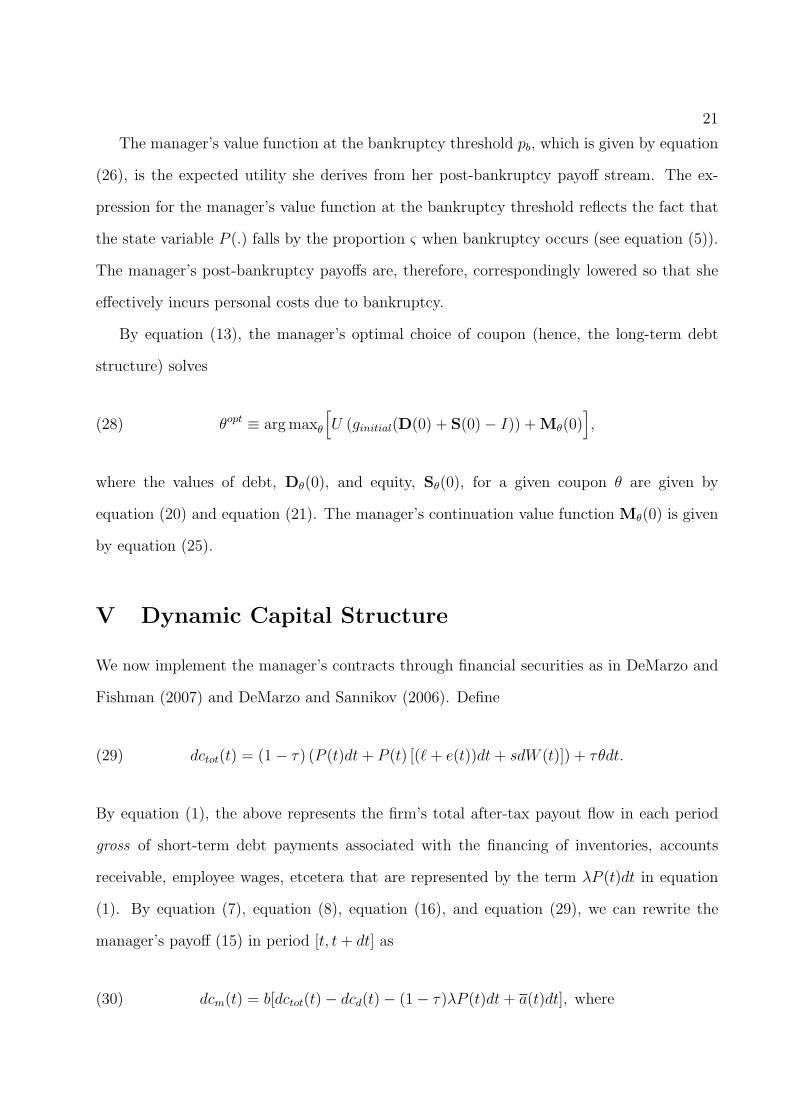
V Dynamic Capital Structure
We now implement the manager’s contracts through financial securities as in DeMarzo and
Fishman (2007) and DeMarzo and Sannikov (2006). Define
(29) dctot(t) = (1− τ) (P (t)dt+ P (t) [(ℓ+ e(t))dt+ sdW (t)]) + τθdt.
By equation (1), the above represents the firm’s total after-tax payout flow in each period
gross of short-term debt payments associated with the financing of inventories, accounts
receivable, employee wages, etcetera that are represented by the term λP (t)dt in equation
(1). By equation (7), equation (8), equation (16), and equation (29), we can rewrite the
manager’s payoff (15) in period [t, t+ dt] as
(30) dcm(t) = b[dctot(t)− dcd(t)− (1− τ)λP (t)dt+ a(t)dt], where
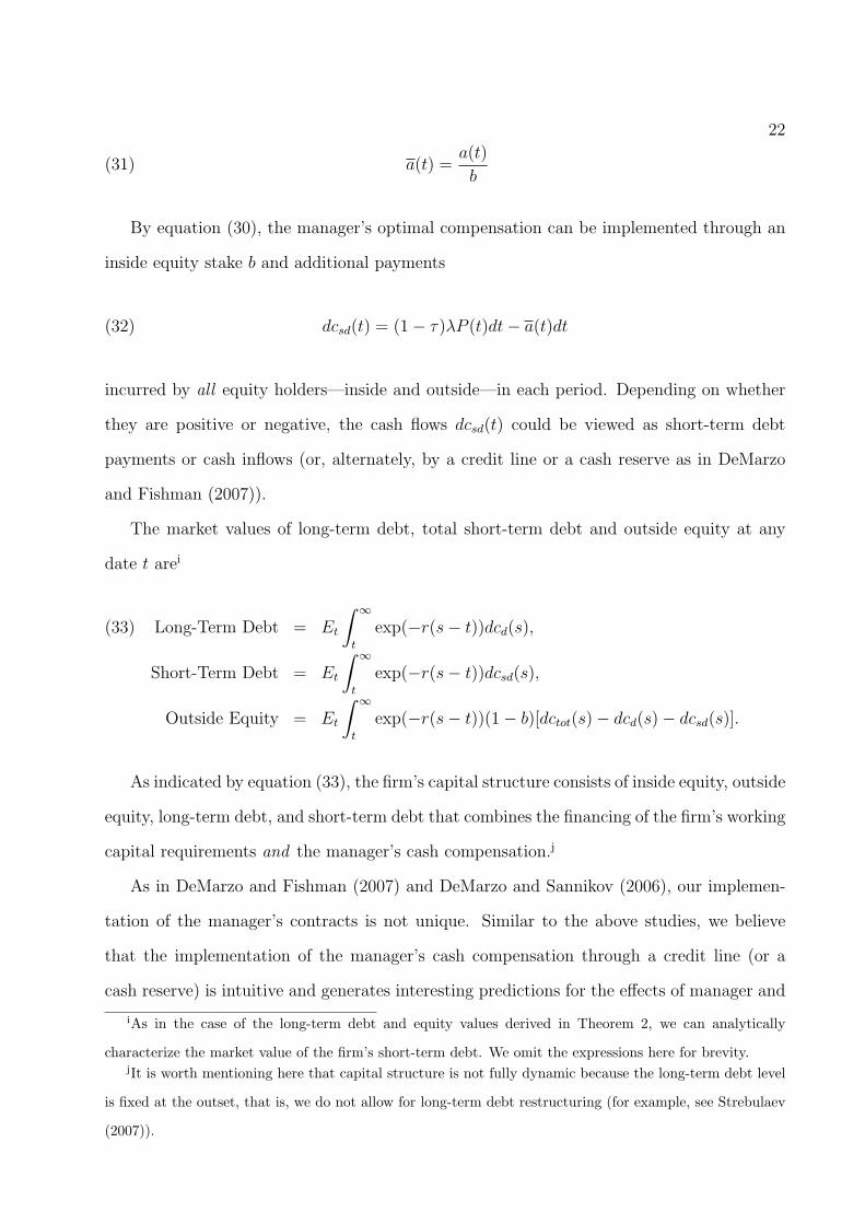
22
(31) a(t) =a(t)
b
By equation (30), the manager’s optimal compensation can be implemented through an
inside equity stake b and additional payments
(32) dcsd(t) = (1− τ)λP (t)dt− a(t)dt
incurred by all equity holders—inside and outside—in each period. Depending on whether
they are positive or negative, the cash flows dcsd(t) could be viewed as short-term debt
payments or cash inflows (or, alternately, by a credit line or a cash reserve as in DeMarzo
and Fishman (2007)).
The market values of long-term debt, total short-term debt and outside equity at any
date t arei
Long-Term Debt = Et
∫ ∞
t
exp(−r(s− t))dcd(s),(33)
Short-Term Debt = Et
∫ ∞
t
exp(−r(s− t))dcsd(s),
Outside Equity = Et
∫ ∞
t
exp(−r(s− t))(1− b)[dctot(s)− dcd(s)− dcsd(s)].
As indicated by equation (33), the firm’s capital structure consists of inside equity, outside
equity, long-term debt, and short-term debt that combines the financing of the firm’s working
capital requirements and the manager’s cash compensation.j
As in DeMarzo and Fishman (2007) and DeMarzo and Sannikov (2006), our implemen-
tation of the manager’s contracts is not unique. Similar to the above studies, we believe
that the implementation of the manager’s cash compensation through a credit line (or a
cash reserve) is intuitive and generates interesting predictions for the effects of manager and
iAs in the case of the long-term debt and equity values derived in Theorem 2, we can analytically
characterize the market value of the firm’s short-term debt. We omit the expressions here for brevity.jIt is worth mentioning here that capital structure is not fully dynamic because the long-term debt level
is fixed at the outset, that is, we do not allow for long-term debt restructuring (for example, see Strebulaev
(2007)).

23
firm characteristics on short-term debt. It is worth emphasizing, however, that the testable
predictions of the model for the effects of manager and firm characteristics on long-term debt
do not depend on our implementation of the manager’s contracts.
VI The Effects of Manager Characteristics
In this section, we investigate the effects of manager characteristics—ability, risk aversion,
and disutility of effort— on the firm’s capital structure. The following theorem analytically
describes the effects of manager characteristics on the firm’s long-term debt.
Theorem 4 (Manager Characteristics, Short-Term Risk, and Long-Term Debt) The
long-term debt value declines with the manager’s ability, increases with her risk aversion,
disutility of effort, and the firm’s short-term risk.
By equation (28), the long-term debt structure is chosen to maximize the sum of the
manager’s initial utility payoff and her continuation value. For a given long-term debt
coupon θ, the manager’s initial utility payoff is U [ginitial(Dθ(0) + Sθ(0)− I)]. As discussed
after Theorem 2, the sum of the market values of long-term debt and equity at date zero,
Dθ(0) + Sθ(0) does not depend on the manager’s ability or effort (see equations (20) and
(21)).
The manager’s optimal choice of long-term debt trades off the beneficial effects of ex post
debt tax shields on her initial payoff from leveraging the firm against the detrimental effects
of debt on the likelihood of bankruptcy and her continuation value. Because the manager’s
risk aversion, disutility of effort, and the firm’s short-term risk only affect her effort (see 16),
it follows from the above discussion that the manager-specific characteristics—ability, risk
aversion, and disutility of effort— and the firm’s short-term risk only affect her continuation
value and not her initial payoff.
As the manager’s ability increases (keeping the debt coupon fixed), the surplus she gen-
erates in each period increases, which increases her continuation value without affecting her
initial payoff. At the margin, she, therefore, cares more about her continuation value rela-
24
tive to her initial payoff. She chooses lower long-term debt, which lowers the likelihood of
bankruptcy and increases her continuation value.
An increase in the manager’s risk aversion, disutility of effort, or the firm’s short-term
risk increases the costs of providing incentives to the manager. She exerts lower effort in equi-
librium, which lowers the surplus she generates in each period. The manager’s continuation
value is lowered relative to her initial payoff. The manager now chooses greater long-term
debt, which increases her initial payoff from leveraging the firm through the exploitation of
ex post debt tax shields. Similarly, an increase in the manager’s discount rate also lowers her
continuation value relative to her initial payoff so that she chooses greater long-term debt.
Casual intuition would suggest that more risk-averse managers would prefer less long-
term debt because the adverse impact of bankruptcy would be greater. The result of the
theorem and the intuition underlying it suggests that this casual intuition is incorrect in our
framework. As discussed above, the manager’s long-term debt choice reflects the tradeoff
between the initial payoff from leveraging the firm and her continuation value. Because
capital markets are competitive so that the manager captures the surplus she generates
from her human capital in each period, the manager’s initial payoff is unaffected by her risk
aversion, while her continuation value is lowered. Consequently, it is optimal for a more
risk-averse manager to increase rather than decrease long-term debt.
As mentioned earlier, the results of Theorem 4 do not depend on our implementation of
the manager’s contracts through financial securities described in Section V. The testable
implications of our theory for the effects of manager and firm characteristics on long-term
debt are, therefore, independent of the choice of implementation of the manager’s contracts.
The effects of manager characteristics on short-term debt are ambiguous for general pa-
rameter values. By equation (16), equation (30), equation (32) and equation (33), short-term
debt decreases with the long-term debt coupon and with the ratio a(t)/b of the parameters
that determine the “cash” and “risky” components of the manager’s compensation (see 15).
By equation (16) and equation (30), an increase in the manager’s ability does not affect
her inside equity stake but increases the cash component of the manager’s compensation,
which has a negative effect on the firm’s short-term debt by equation (32) and equation
25
(33). Recall that the long-term debt coupon also decreases with the manager’s ability, which
has a positive effect on the firm’s short-term debt by equation (16), equation (30), equation
(32) and equation (33). For general parameter values, therefore, the effect of managerial
ability on the firm’s short-term debt is ambiguous. By similar arguments, the effects of the
risk aversion, γ, and disutility of effort, κ, on short-term debt are also ambiguous. In the
next sub-section, we numerically explore the effects of manager characteristics on short-term
debt.k
A Numerical Analysis
In this section, we conduct a quantitative investigation of the effects of manager and firm
characteristics on capital structure. To examine the robustness of our implications, we
have numerically investigated the basic model of Section III as well as the extended model
described in Appendix B in which the manager continues servicing debt even after the
equity value falls to zero. Because our key testable implications are unchanged, we present
the results of our analysis of the basic model.
Model Calibration
To obtain a reasonable set of baseline parameter values, we calibrate the parameters of the
model to the data we use for our subsequent empirical analysis.
Risk-Free Rate, Tax Rate, Bankruptcy Costs : We set the risk-free rate r to 6.0% and
the effective corporate tax rate τ to 0.15, which is consistent with the estimates of Goldstein
et al. (2001).l We set the proportional bankruptcy cost parameter ς to 0.15, which is the
kIt is important to emphasize here that the results of Theorem 4 rely on the assumption that managerial
ability does not have long-term effects on earnings. As suggested by the intuition above, if ability were
to have long-term effects on earnings by (for example) affecting the drift of the state variable P (.), the
implications of the theorem could change. However, the fact that we find strong empirical support for the
implications of the theorem suggests that the effects of managerial ability on earnings is short-term.lRecall that we assume that taxation is symmetric for simplicity. The effective corporate tax rate also
incorporates the effects of personal taxes. An effective corporate tax rate of 0.15 is consistent with the
estimates of the tax advantage of debt using corporate tax rates as well as personal tax rates on interest and

26
midpoint of the range [0.10, 0.20] of proportional financial distress costs reported in Andrade
and Kaplan (1998).
Short-Term Risk, Long-Term Risk, Drift, Initial EBITM Rate, and Invest-
ment : Our proxy for the asset value is the value of the un-levered firm net of the manager’s
contractual compensation. It follows from equation (1), equation (2) and Theorem 1 that
the asset value A(t) at any date t is the present value of the stream of after-tax earnings
from existing assets,
(34) A(t) = Et
[∫ ∞
t
exp (−r(u− t)) (1− τ)P (u)du
]=
(1− τ)P (t)
r − µ.
We set the initial investment outlay I equal to the asset value at date zero. We normalize
the initial EBITM rate P (0) so that the asset value or book value is 100.
The average after-tax annual return on assets is the ratio of average annual after-tax
earnings net of the manager’s contractual compensation to asset value. By equation (1)
and equation (34), this is equal to (1−τ)P (t)A(t)
= r − µ. Since r = 0.06, we set µ = −0.02 to
approximately match the median annual after-tax earnings to asset value ratio in our sample.
Note that, as discussed in Leland (1998) and Chapter 12 of Duffie (2001), the assumption
that investors are risk-neutral implicitly means that we are carrying out our analysis under
the risk-neutral probability. Therefore, the parameter µ is, in fact, the risk-neutral drift of
the state variable P (.). Since the risk-neutral drift equals the actual drift (the drift under
the physical or “real world” probability) less the risk premium, it could be negative.
From equation (1) and equation (34), the standard deviation of the after-tax return on
assets is (r− µ) ∗ s. The median of the standard deviations of the after-tax return on assets
in our sample is approximately 0.015. Accordingly, we set s = 0.015r−µ
≈ 0.19. We set the
long-term risk, σ, to its median value in our sample, 0.29.
Manager Variables: The median CEO percentage ownership (including options adjusted
by their respective deltas) in the sample we use for our empirical analysis is approximately
0.035 (see Table 5). Accordingly, we set the manager’s initial equity ownership ginitial to
dividend income.
27
0.035. We calibrate the baseline values of the manager’s ability ℓ, risk aversion γ, discount
rate β, disutility of effort κ, and the parameter λ associated with the short-term debt financ-
ing of the firm’s working capital requirements (see 1) by matching key, relevant statistics
predicted by the model to their median values in the data. Specifically, we indirectly de-
termine the parameters so that (i) the manager’s inside equity stake; (ii) the ratio of the
manager’s cash compensation to asset value; (iii) the ratio of the firm’s net short-term debt
(short-term debt net of cash) to asset value; (iv) the ratio of long-term debt to asset value;
and (v) the ratio of firm value to asset value match the median CEO equity stake, the median
ratio of CEO cash compensation to asset value, the median net short-term debt ratio, the
median long-term debt ratio, and the median ratio of firm value to asset value, respectively,
in the data.
We calculate a firm’s net short-term debt as “debt in current liabilities”, which includes
lines of credit (Compustat item #34) minus “debt due in one year” (Compustat item #44)
minus cash (Compustat item #1). We subtract item #44 from item #34 to correspond as
closely as possible to the short-term debt measure in the theoretical model because both
items include current portions of long-term debt, while item #34 includes lines of credit.m
From Table 5, the median ratio of net short-term debt to asset value for the firms in our
sample is 8.2% and the median ratio of long-term debt (Compustat item #9) to asset value is
15.5%. The median ratio of firm value to asset value in our sample is 1.16. The median ratio
of the annual cash compensation of CEOs to asset value for firms in our sample is 0.075%.
(Note that the ratio of the present value of the stream of future CEO cash compensation
payments to asset value is an order of magnitude higher.)
Baseline Parameter Values: Table 2 lists the baseline values of all the parameters in
the model. Table 3 shows the baseline firm value, long-term debt ratio and net short-term
debt ratio. Note that the firm value is the market value of the firm’s stream of total after-tax
earnings and, therefore, includes the manager’s stake. We normalize the initial value P (0)
of the state variable so that the asset value (the un-levered firm value net of the manager’s
stake) defined in equation (34) is 100.
mOur results are not altered if we do not subtract item #44 in the calculation of net short-term debt.
28
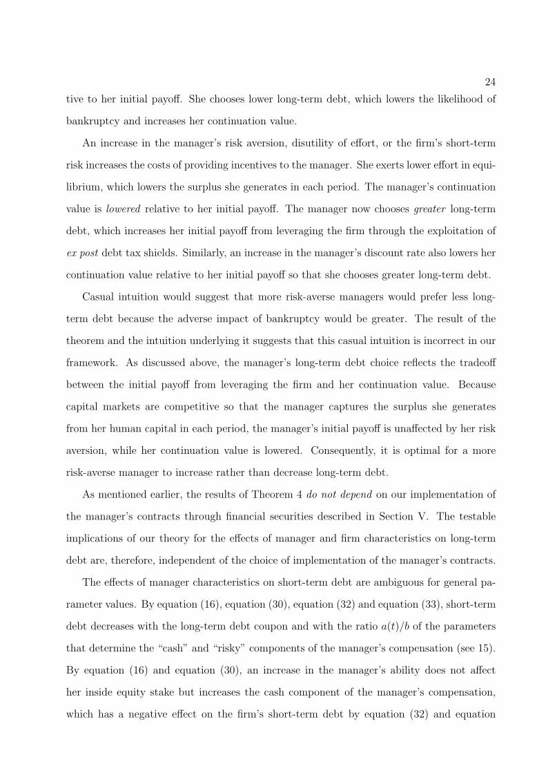
The Effects of Manager Characteristics
The Effects of the Manager’s Ability
Figure 1 displays the variation of the long-term, short-term and total debt ratios with the
manager’s ability ℓ. Consistent with Theorem 4, long-term debt declines with the manager’s
ability. For the baseline values of the other model parameters, the figure shows that the
negative effects of an increase in ability on short-term debt dominate the positive effects
so that short-term debt declines with ability (recall the discussion following Theorem 4).
As the manager’s ability increases, the firm moves from holding positive short-term debt to
holding cash. The total debt ratio also declines with manager ability because the long-term
and short-term debt ratios decline.
PLACE FIGURE 1 ABOUT HERE
The Effects of the Manager’s Risk Aversion
Figure 2 shows the effects of the manager’s risk aversion γ. Consistent with Theorem
4, long-term debt increases with the manager’s risk aversion. The table shows that short-
term debt decreases with the manager’s risk aversion in the calibrated model. As the risk
aversion increases, it is costlier to provide incentives to the manager. Hence, the “power of
incentives” represented by the manager’s inside equity stake declines (see equations (16) and
(30)). Consequently, the manager receives a greater portion of her compensation in cash so
that the firm’s short-term debt decreases (see equation (32)). The decline in short-term debt
with risk aversion dominates the increase in long-term debt so that the total debt ratio also
decreases.
PLACE FIGURE 2 ABOUT HERE
Because the manager’s inside equity stake declines with her risk aversion, the results
imply that the long-term debt ratio declines with the manager’s inside equity stake, while
the short-term debt ratio increases. The In unreported results, the effects of the manager’s
disutility of effort are similar to those of the manager’s risk aversion. The effects of the two
29
variables are qualitatively similar because an increase in either κ or γ increases the costs of
providing incentives to the manager.
We remind the reader here that short-term debt in the model is determined by the firm’s
working capital requirements and the manager’s (more generally, insiders’) cash compen-
sation. As discussed above, manager-specific characteristics affect short-term debt through
their effects on the manager’s cash compensation.
The Effects of Short-Term Risk
Figure 3 shows the effects of the short-term risk s. Short-term risk has differing effects on the
firm’s long-term and short-term debt. Consistent with Theorem 4, long-term debt increases
with short-term risk. Short-term debt, however, decreases. By Theorem 1 and equation
(16), an increase in the short-term risk lowers the power of incentives to the manager, and
increases the “cash” portion of her compensation. By equation (32) and equation (33), this
has a negative effect on the firm’s short-term debt. The decline in short-term debt with
short-term risk dominates the increase in long-term debt so that the total debt ratio also
decreases.
PLACE FIGURE 3 ABOUT HERE
The Effects of Long-Term Risk
Figure 4 shows the effects of the firm’s long-term risk, σ. The firm’s long-term risk also
has differing effects on long-term and short-term debt. By the discussion in Section A, the
manager’s choice of long-term debt reflects its effects on her initial payoff and her continu-
ation value by equation (28). By equation (16), the long-term risk σ has no effect on the
manager’s compensation structure and, therefore, on the output she generates in each pe-
riod. The manager’s continuation value, however, declines with the long-term risk because
it increases the likelihood of bankruptcy and the associated personal costs for the manager.
Long-term debt therefore declines with long-term risk.
PLACE FIGURE 4 ABOUT HERE

30
The decline in the long-term debt coupon with long-term risk has a positive effect on
the firm’s short-term debt (see equations (16), (30), and (32)). The increased likelihood of
bankruptcy, however, has a negative effect on the value of the firm’s short-term debt. The
interplay between these two effects causes short-term debt to vary non-monotonically with
long-term risk.
Comparing Figures 3 and 4, we conclude that distinct components of the firm’s risk
have differing effects on its capital structure. The differing effects arise due to the fact
that short-term risk directly affects the manager’s incentive compensation in each period.
The long-term risk, on the other hand, has longer-term effects by influencing the manager’s
valuation of her stream of future payoffs and the likelihood of bankruptcy.
The incorporation of managerial discretion and risk aversion in our model plays a central
role in generating the differing effects of long-term risk and short-term risk on the firm’s debt
structure. In addition to the predicted effects of manager characteristics on capital struc-
ture, these results distinguish our theory from theories that do not incorporate managerial
discretion or risk aversion.
Effects of Manager’s Initial Stake
Figure 5 shows the effects of varying the manager’s initial stake ginitial. Long-term debt
increases with the manager’s initial stake, short-term debt declines, and total debt increases.
By equation (13), an increase in the manager’s initial stake increases her payoff from external
financing at date zero, but does not affect her continuation value by equation (25) and
equation (26). Consequently, she chooses greater long-term debt. By equation (16), equation
(31) and equation (32), an increase in the long-term debt coupon lowers short-term debt.
In the calibrated model, the increase in long-term debt more than offsets the decline in
short-term debt so that total debt increases.
The Effects of Bargaining Power
In the analysis thus far, we assumed that capital markets are competitive so that the manager
appropriates the surplus she generates from her human capital. We now explore the robust-
31
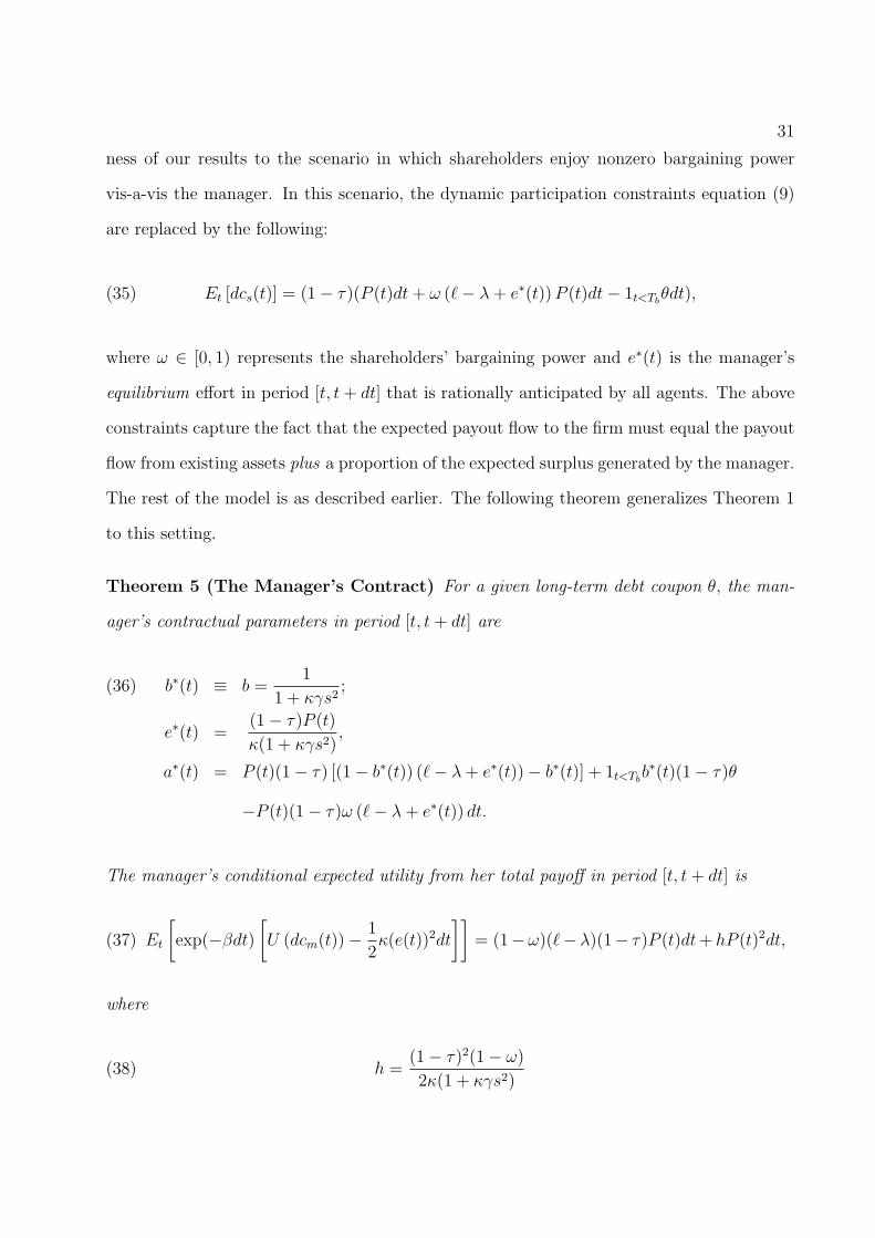
ness of our results to the scenario in which shareholders enjoy nonzero bargaining power
vis-a-vis the manager. In this scenario, the dynamic participation constraints equation (9)
are replaced by the following:
(35) Et [dcs(t)] = (1− τ)(P (t)dt+ ω (ℓ− λ+ e∗(t))P (t)dt− 1t<Tbθdt),
where ω ∈ [0, 1) represents the shareholders’ bargaining power and e∗(t) is the manager’s
equilibrium effort in period [t, t+ dt] that is rationally anticipated by all agents. The above
constraints capture the fact that the expected payout flow to the firm must equal the payout
flow from existing assets plus a proportion of the expected surplus generated by the manager.
The rest of the model is as described earlier. The following theorem generalizes Theorem 1
to this setting.
Theorem 5 (The Manager’s Contract) For a given long-term debt coupon θ, the man-
ager’s contractual parameters in period [t, t+ dt] are
b∗(t) ≡ b =1
1 + κγs2;(36)
e∗(t) =(1− τ)P (t)
κ(1 + κγs2),
a∗(t) = P (t)(1− τ) [(1− b∗(t)) (ℓ− λ+ e∗(t))− b∗(t)] + 1t<Tbb∗(t)(1− τ)θ
−P (t)(1− τ)ω (ℓ− λ+ e∗(t)) dt.
The manager’s conditional expected utility from her total payoff in period [t, t+ dt] is
(37) Et
[exp(−βdt)
[U (dcm(t))−
1
2κ(e(t))2dt
]]= (1−ω)(ℓ− λ)(1− τ)P (t)dt+ hP (t)2dt,
where
(38) h =(1− τ)2(1− ω)
2κ(1 + κγs2)
32
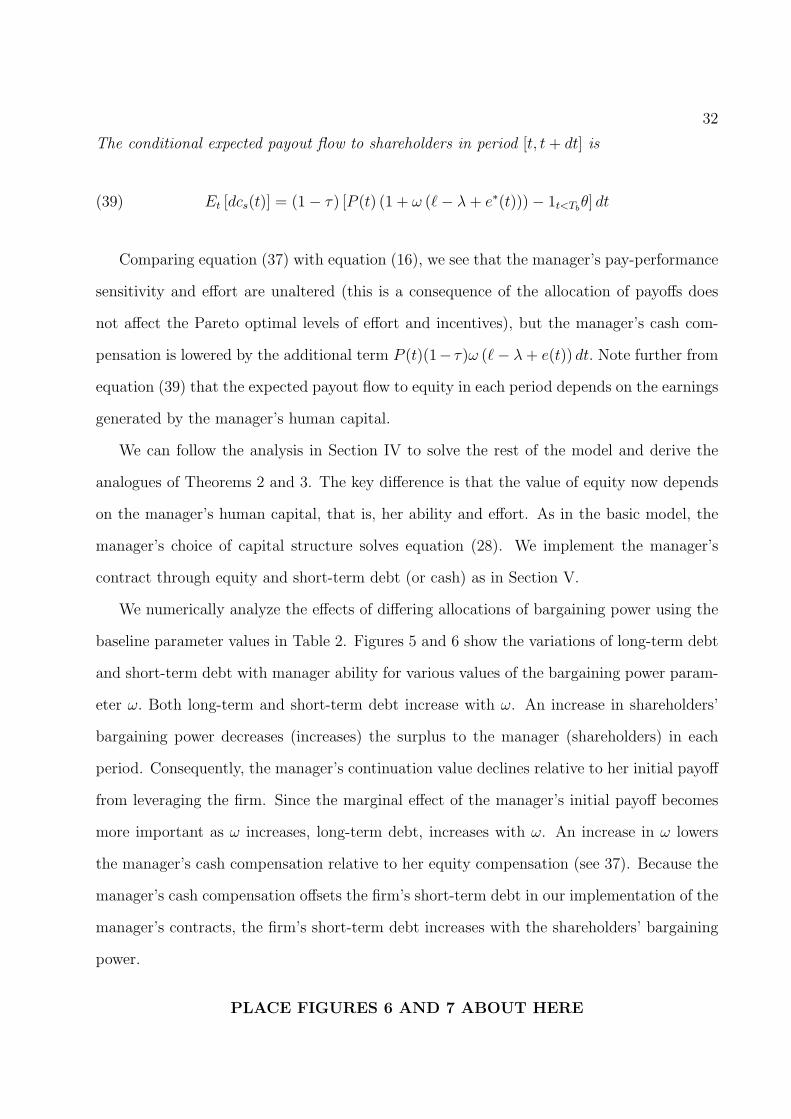
The conditional expected payout flow to shareholders in period [t, t+ dt] is
(39) Et [dcs(t)] = (1− τ) [P (t) (1 + ω (ℓ− λ+ e∗(t)))− 1t<Tbθ] dt
Comparing equation (37) with equation (16), we see that the manager’s pay-performance
sensitivity and effort are unaltered (this is a consequence of the allocation of payoffs does
not affect the Pareto optimal levels of effort and incentives), but the manager’s cash com-
pensation is lowered by the additional term P (t)(1− τ)ω (ℓ− λ+ e(t)) dt. Note further from
equation (39) that the expected payout flow to equity in each period depends on the earnings
generated by the manager’s human capital.
We can follow the analysis in Section IV to solve the rest of the model and derive the
analogues of Theorems 2 and 3. The key difference is that the value of equity now depends
on the manager’s human capital, that is, her ability and effort. As in the basic model, the
manager’s choice of capital structure solves equation (28). We implement the manager’s
contract through equity and short-term debt (or cash) as in Section V.
We numerically analyze the effects of differing allocations of bargaining power using the
baseline parameter values in Table 2. Figures 5 and 6 show the variations of long-term debt
and short-term debt with manager ability for various values of the bargaining power param-
eter ω. Both long-term and short-term debt increase with ω. An increase in shareholders’
bargaining power decreases (increases) the surplus to the manager (shareholders) in each
period. Consequently, the manager’s continuation value declines relative to her initial payoff
from leveraging the firm. Since the marginal effect of the manager’s initial payoff becomes
more important as ω increases, long-term debt, increases with ω. An increase in ω lowers
the manager’s cash compensation relative to her equity compensation (see 37). Because the
manager’s cash compensation offsets the firm’s short-term debt in our implementation of the
manager’s contracts, the firm’s short-term debt increases with the shareholders’ bargaining
power.
PLACE FIGURES 6 AND 7 ABOUT HERE
33
Figures 6 and 7 show that our earlier implications for the variations of long-term debt
and short-term debt with manager ability are generally robust to variations of the bargaining
power of shareholders vis-a-vis the manager. Short-term debt always declines with manager
ability. Long-term debt also declines as long as ω is not too high. When ω is above a
threshold, long-term debt declines with ability below a threshold and then increases. The
underlying intuition is the following. As discussed above, an increase in ω increases the
relative effects of the manager’s initial payoff on her long-term debt choice. These effects
are further accentuated when the manager’s ability is above a threshold. For high values
of ω and when the manager’s ability is above a threshold, therefore, long-term debt could
increase with manager ability. Overall, our results, therefore, suggest that long-term debt
declines with manager ability unless shareholders’ bargaining power vis-a-vis the manager
and the manager’s ability are both high.
The implications of the basic model for the variations of debt structure with manager risk
aversion, long-term risk, and short-term risk are also robust to variations in the shareholders’
bargaining power ω. We do not display these results for brevity.
VII Empirical Analysis
A Testable Hypotheses
The results of Section VI lead to the seven empirically testable hypotheses shown in Table 1.
In reality, capital structure is potentially affected by several variables that are not present in
our stylized model. In our empirical analysis, therefore, we test our hypotheses controlling
for the effects of the various other determinants of capital structure identified by previous
empirical studies.
PLACE TABLE 1 ABOUT HERE
34
B Data
Our sample includes firms with available data, as detailed below, from Compustat, Execu-
comp, IRRC, and CRSP over the period 1993-2007. All variables are described in Table
4.
Leverage Variables: A firm’s long-term debt ratio is its long-term debt (Compustat item
#9) scaled by total assets (Compustat item #5). A firm’s short-term debt ratio is short-term
debt minus cash (the net short-term debt) scaled by total assets. We calculate a firm’s net
short-term debt as its “debt in current liabilities” (Compustat item #34) - “debt due in one
year” (item #44) - “cash” (item #1). We subtract item #44 because both items #34 and
#44 include current portions of long-term debt, while item #34 includes lines of credit that
are not included in item #44. By subtracting item #44 from item #34, we exclude portions
of the firm’s long-term debt from the short-term debt measure, which is consistent with the
model. We have also run our tests without subtracting item #44 and obtain very similar
results. We mention here that our proxy for short-term debt is not working capital.
CEO Ability : We construct five proxies of CEO ability for robustness. The first three
proxies are directly derived from the theory, while the last two are indirect proxies.
a) CEO Cash Compensation: By equation (16) and equation (31), the manager’s cash
compensation increases with her ability. Our first proxy for CEO ability is therefore the
cash compensation of the CEO. The use of cash compensation as a proxy for ability is also
consistent with neo-classical models in which agents are paid their marginal products.
b) CEO Cash Compensation to Assets Ratio: To control for possible “size” effects on
compensation, we also use the ratio of CEO cash compensation to assets as a proxy for CEO
ability.
c) Industry adjusted accounting performance: To the extent that a CEO of superior abil-
ity delivers superior corporate performance, CEO ability and industry adjusted accounting
performance are likely to be significantly positively correlated. Consistent with this intu-
ition, the manager’s ability positively affects earnings in our model (see 1). Our third proxy
of CEO ability is the industry-adjusted return on assets of the firm, that is, the excess return
35
on assets of the firm relative to other firms in the same 4-digit SIC industry. We consider
accounting, rather than stock market, measures of performance since an efficient stock mar-
ket would anticipate the impact of CEO ability on the firm and impound it into the share
price.
d) CEO tenure: In our model, a CEO of superior ability delivers superior corporate
performance. Also, a significant body of literature in finance and accounting has documented
disciplinary CEO turnover subsequent to poor performance (e.g. see Farrell and Whidbee,
2003). Hence, CEO ability is likely positively correlated with CEO tenure.
e) CEO tenure divided by CEO age. Consider two CEOs, A and B, who have both served
as CEOs for five years. A is 55 years old, and B is 65. It is plausible that, ceteris paribus,
A has greater ability than B, since she has accomplished/survived a five year tenure at an
earlier age. Accordingly, we use CEO tenure/CEO age as our third proxy for CEO ability.n
CEO Ownership: We calculate a CEO’s equity ownership in the firm using the number
of shares of common stock and the number of options held by the CEO. Specifically, the
CEO’s percentage ownership at any date is equal to the number of shares of company stock
she holds plus the number of options weighted by their respective deltas. We have also run
our tests using CEO dollar ownership measures and obtained very similar results.
Long-Term Risk and Short-Term Risk : Consistent with the model, we measure short-
term risk as the standard deviation of the quarterly return on assets over the past three years
(see 1). Consistent with equation (2), we measure long-term risk as the standard deviation
of the logarithm of firm value over the past three years. For robustness, we also run our tests
using the 3-year standard deviation of the quarterly earnings per share (EPS) as the proxy
for short-term risk, and the 3-year standard deviation of monthly stock returns as the proxy
for long-term risk. Our results remain robust to these alternate proxies.o Table 5 presents
nAs robustness checks, we have also run our tests with the following alternate measures of CEO ability:
(i) CEO Tenure and CEO Tenure/CEO Age with minimum cutoffs for tenure of 2, 3, and 4 years; (ii)
unadjusted ROA; (iii) CEO Tenure and CEO Tenure/CEO Age for cumulative tenure as a CEO, not just
as a CEO of the sample firm; and (iv) average annual adjusted ROA during the current CEO’s tenure. Our
results are qualitatively unaltered.oAs additional robustness checks, we have also run our tests with long-term risk measured as the standard

36
the descriptive statistics for the variables.
PLACE Table 5 ABOUT HERE
C Manager Ability and Debt Structure
Table 6 shows the empirical relationship between debt structure and our proxies for man-
agerial ability. We report ordinary least squares regression results with firm fixed effects.
Standard errors of coefficient estimates are corrected for clustering at the firm level.
PLACE Table 6 ABOUT HERE
Consider Table 6, Panel A. Regressions 1-3 include only the control variables motivated
by the extensive capital structure literature. Consistent with the extant literature we find
that asset tangibility and firm size positively affect leverage. Growth opportunities and
firm profitability are negatively related to leverage. Regression 3 includes the past three
years’ stock returns; past stock returns are negatively correlated with leverage. Tangibility
of assets, growth opportunities, and firm profitability are significantly correlated within an
industry group. Hence, when we include industry leverage as a control in Regression 2, the
above three control variables’ coefficients diminish in magnitude.
Given the above findings, we include firm size, industry leverage, and past stock returns
as the control variables in the remaining regression models. Regression 4, 5 and 6 in Table
6, Panel A, document the significant negative relations between the long-term debt ratio
and the direct proxies of CEO ability; CEO cash compensation, the ratio of CEO cash
compensation to assets, and the industry adjusted return on assets. Regressions 7 and 8
show the significant negative relations between the long-term debt ratio and the indirect
proxies of CEO ability: CEO tenure and the ratio of CEO tenure to age. Consistent with
Hypothesis 1 in Table 1, therefore, the long term debt ratio declines with managerial ability.
deviation of monthly returns over the past 5 years; and short-term risk measured as the standard deviation
of 3-5 year return on assets as well as 3-5 year standard deviation of the P-E ratio. Our results are unaltered.
37
Consistent with Hypothesis 2 in Table 1, regressions 4-8 in Table 6, Panel B, document a
negative relation between short-term debt and our proxies for managerial ability. The neg-
ative relation between short-term debt and CEO cash compensation also provides empirical
support for our implementation of the manager’s contracts in which an increase in the CEO’s
cash compensation has a negative effect on short-term debt (see 32).
The effects of CEO ability on debt structure are also economically significant. Using
cash compensation as the measure of manager ability, a 1% increase in managerial ability is
associated with a 0.11% decline in long-term debt and a 0.38% decline in short-term debt.pAs
a point of comparison, the elasticity of past stock returns to the long-term debt ratio is -
0.03%; that is, a 1% increase in past stock returns is associated with a 0.03% decrease in the
long-term debt ratio.
D Manager Ownership and Debt Structure
As mentioned in Section B, the manager’s ownership stake includes stock and option compen-
sation. The results in Table 7, Panel A, regressions 1 and 2 are consistent with Hypothesis
3 in Table 1. The long-term debt ratio decreases with the CEO’s ownership stake.
Regressions 3-7 in Table 7, Panel A include our five proxies of manager ability as controls.
Consistent with the results of Table 6, long term debt is negatively related to each of the five
proxies of managerial ability. After including manager ability as a control, we continue to
find a negative and statistically significant relation between the long-term debt ratio and the
manager’s inside equity stake. These results are also economically significant. For example,
a 1% increase in the manager’s equity stake is associated with a 0.04% decline in long-term
debt.
PLACE Table 7 ABOUT HERE
The results in Table 7, Panel B, regressions 1-7 indicate a statistically insignificant or
marginally significant negative relation between the manager’s equity stake and the short-
pUsing other variables for managerial ability, the economic significance of the effect of ability on debt
structure is of comparable magnitude.
38
term debt ratio. We, therefore, do not find empirical support for Hypothesis 4 in Table
1.
E Long-Term Risk, Short-Term Risk, and Debt Structure
We find a statistically significant negative relation between the long-term debt ratio and
long-term risk in Table 6, Panel A, and Table 7, Panel A. We also document a statistically
significant and positive relation between the long-term debt ratio and short-term risk in
Table 6, Panel A, and Table 7, Panel A. These results are consistent with Hypothesis 5 and
Hypothesis 6 in Table 1.
Consistent with Hypothesis 7, Table 6, Panel B and Table 7, Panel B show that the
relation between short-term debt and short-term risk is negative. Our empirical results also
show that the relation between short-term debt and long-term risk is negative.
F Endogeneity
Manager ownership and capital structure are simultaneously and endogenously determined in
the model, which could potentially lead to biased and inconsistent OLS coefficients in Table 7.
To address these issues, we use instrumental variables and two-stage least squares regression
analysis (2SLS). The primary instrumental variable that we use for manager ownership is
the average ownership of CEOs in the same four-digit SIC code. We also include the vector
of control variables from the second stage leverage regression as additional instruments in
the first stage. Specifically, the first stage regression that we run is the following:
CEO ownershipi,t =f(Average industry CEO ownershipi,t, LnAssetsi,t,(40)
Advertising and R&D expensesi,t, Past stock returnsi,t,
Market-to-Booki,t, Long-term riski,t, Short-term riski,t)
We use this equation to obtain a predicted value for CEO Ownership. We use this
predicted value in our second stage leverage regression along with the other control variables

39
in the regressions in Table 7. We test the appropriateness of our first stage instruments
using a battery of specification tests. First, we use the Stock and Yogo (2005) test for
weak instruments. This is a test of the strength of the instruments included in the first
stage regression, but not included in the second stage regression to determine how much
information is added to the predicted value by the instruments (see also Cragg and Donald,
1993). In our regression model, these instruments include Average Industry CEO Ownership,
Advertising and R& D expenses, and Market-to-Book ratio. Second, we use the Hahn and
Hausman (2002) test for instrument validity to verify that the instruments are not correlated
with capital structure.q In unreported results, we find that these instruments are indeed
valid, suggesting that the model is not affected by any correlation between our instruments
and capital structure. While these two diagnostic tests suggest that our choice of instruments
is appropriate for this model, for completeness we also perform the Anderson-Rubin test and
the Hansen-Sargan test.r Both of these tests show that our system of equation is properly
identified, suggesting that our instruments are appropriate.sMore specifically, the Hansen-
Sargan test results fail to reject the null hypothesis that there is no correlation between the
exogenous instruments and the error term from the capital structure equations.tThe results
of these tests show that our choice of instruments is indeed appropriate. Finally, we test
qThe Spearman rank correlation between average industry CEO ownership and long term debt is 0.10;
the Spearman rank correlation between average industry CEO ownership and short term debt is 0.07.rThe Hansen-Sargan test is a test for overidentifying restrictions, testing the joint significance of the
set of endogenous variables in the system of equations. It has a Chi-square distribution (with degrees of
freedom equal to the number of instruments minus the number of parameters), and the null hypothesis is
that the instruments are valid. Large p-values suggest that the instruments are valid. The Anderson-Rubin
(1949, 1950) test is a test of the joint significance of a set of endogenous variables in a system of equations.
It tests for the joint significance of the excluded instruments by substituting the first-stage reduced-form
equations into the second-stage structural equations. The test statistic has a Chi-square distribution; large
test statistics and small p-values suggest instrument validity and joint significance of the system.sWe establish a system of equations only to perform these two identification tests. We are not concerned
about the effect that capital structure has on manager ownership, and so we do not analyze or discuss that
relationship.tThe p-values for the Hansen-Sargan tests are all greater than 0.28 and the p-values for the Anderson-
Rubin test are all less than 0.06.
40
whether or not endogeneity is an issue in our system using the Hausman (1978) specification
test. The results from this test suggest that our system is weakly affected by endogeneity
(p-values around 0.10).
Table 8 presents the results from the second-stage leverage regressions. The results are
consistent with those in Table 7 and show that, with the exception of the predicted relation
between short-term debt and manager ownership, the testable hypotheses hold even after
adjusting for endogeneity.
PLACE TABLE 8 ABOUT HERE
G Manager Characteristics and Incremental Debt Financing
Strebulaev (2007) argues that leverage panel regressions similar to the ones above could be
misspecified in a dynamic context because firms rebalance their debt only infrequently in
the presence of adjustment costs. Consequently, firms could be at different points in their
refinancing cycles even though they are otherwise identical, which complicates the inferences
from such regressions. He argues for a structural approach to the empirical analysis of firms’
capital structure decisions. While a fully structural approach is beyond the scope of this
paper, we take some steps towards addressing his critique by analyzing the incremental
financing decisions of firms.
We collect external financing data: the net issuance of long-term debt (Compustat item
# 111 - item # 114); the net issuance of short-term debt (the change in current liabilities,
Compustat item #5, adjusted for long-term debt in current liabilities, Compustat item #34);
and the net issuance of common stocks and preferred stocks (Compustat item # 108 - item #
115). A negative value for the net issuance of debt and equity during a particular fiscal year
implies that the firm effectively buys back outstanding securities during that year. To focus
on the financing of new investments, we restrict consideration to firm-year samples where the
net issuance of equity and debt are both nonnegative. The sample for these tests, therefore,
includes firm-year observations with external financing and excludes those corresponding to
securities buy-backs.
41
The dependent variable in the tests is the proportion of incremental long-term debt fi-
nancing or the proportion of incremental short-term debt financing to total external financing
for each firm-year observation. The independent variables in our tests are the same as those
in Tables 6 and 7, respectively. Table 9 displays the results. From Panels A and B, we
see that, consistent with our hypotheses, manager ability and ownership negatively affect
the proportion of incremental long-term debt financing. From Panels C and D, measures of
managerial ability negatively affect the proportion of incremental short-term debt financing.
PLACE TABLE 9 ABOUT HERE
VIII Conclusions
We theoretically and empirically investigate the effects of manager characteristics on capital
structure. We develop a dynamic principal-agent model that incorporates taxes, bankruptcy
costs, and managerial discretion in financing and effort. We derive the manager’s dynamic
contract and implement it through financial securities, which leads to a dynamic capital
structure for the firm.
We derive novel implications that link manager and firm characteristics to capital struc-
ture: (i) Long-term debt declines with manager ability, and with her inside equity ownership.
(ii) Short-term debt declines with manager ability, and increases with her equity ownership.
(iii) Long-term debt declines with long-term risk, and increases with short-term risk. (iv)
Short-term debt declines with short-term risk. With the exception of the relation between
short-term debt and manager ownership, we show empirical support for the above implica-
tions. Our results show that manager characteristics are important determinants of firms’
financial policies.
In this study, we consider a framework with limited commitment in which only single
period contracts are enforceable. The generalization to the scenario in which long-term
contracts are feasible is significantly more complex. In fact, in the current setup where
the manager is risk-averse, earnings have unbounded support, the manager’s effort can take
a continuum of values, and the relationship can be endogenously terminated, it is unclear
42
whether a framework with long-term contracting is analytically or computationally tractable.
This is because, as shown by the dynamic contracting literature, the manager’s continuation
value is an additional state variable that can take a continuum of values. Further, the
risk aversion of the manager makes the optimal contracting problem non-concave unless
one allows for public randomization. An additional major complication is that there are
external frictions due to taxes and bankruptcy costs. Recent studies that allow for long-
term contracting such as DeMarzo and Sannikov (2006) and DeMarzo and Fishman (2007)
obtain tractability with simplifying assumptions such as zero taxes, universal risk-neutrality,
a linear disutility of effort so that a “bang bang” solution for the manager’s effort choice
problem is optimal, and the assumption that is always optimal to implement maximal effort
by the manager. The analysis of a fairly general long-term contracting model with managerial
risk aversion, taxes and bankruptcy costs is a major challenge for future research.
Appendix A
Proof of Theorem 1
a) Because only single-period contracts are enforceable, the contract Γ must be sequentially
optimal, that is, it must be optimal in every continuation game corresponding to all dates
and histories. Suppose that there is nonzero slack in the constraint (9) at some date t for a
Ft-measurable set A. We can construct a new contract Γ′ that modifies Γ by increasing the
manager’s payoff in period [t, t+ dt] by ϵ > 0 conditional on the prior history at date t lying
in the set A. For a sufficiently small ϵ, the participation constraints are satisfied at date t.
They are clearly satisfied at all subsequent dates because Γ′ is identical to Γ at these dates.
Therefore, the manager’s valuation of her future payoff stream under Γ′ is strictly greater
than the valuation under Γ at date t so that Γ is not sequentially optimal. Because the date
t and the set A are arbitrary, the dynamic constraints equation (9) must be satisfied with
equality at each date and state.
Suppose the manager’s contractual parameters (defined in 15) in period [t, t + dt] when
the firm is solvent are (a, b) and the manager exerts effort e. It immediately follows from
43
equation (9) that the following period by period “after tax” constraints must be satisfied:
Ee
[dcs(t)|Ft
]=
((1− τ)(P (t)− θ)dt
), t < Tb,(A-1)
Ee
[dcs(t)|Ft
]=
((1− τ)P (t)dt
), t ≥ Tb.
The manager’s payoff in the period [t, t+ dt] is
dcm(t) = adt+ b(1− τ)[dQ(t)− 1t<Tbθdt].
By equation (1), equation (3), and equation (4), the manager’s conditional expected utility
from her payoff over the period [t, t+ dt] is
(A-2)
m(a,b,e)(t) = adt−b(1−τ)1t<Tbθdt+b(1−τ)P (t)(1+ℓ−λ+e)dt−1
2κe2dt−1
2γ(1−τ)2b2s2P (t)2dt,
where the subscripts indicate the dependence of the manager’s conditional expected utility
on the contractual parameters (a, b, e). Using standard dynamic programming arguments,
the manager’s optimal value function at at date t must satisfy the following formal dynamic
programming equation:
(A-3) M(t) = sup(a,b,e)
m(a,B,e)(t) + Ete−rdtM(t+ dt),
where the optimization is subject to the constraint equation (A-2). Since the manager’s effort
only affects her payoffs in the current period, and her contract must be sequentially optimal,
the manager’s optimal continuation value M(t + dt) does not depend on the contractual
parameters (a, b, e). Hence, the manager chooses these parameters to maximize m(a,b,e)(t)
subject to the constraint equation (A-2).
We first determine the manager’s optimal effort given the compensation parameters (a, b).
It follows directly from equation (A-2) that the manager’s incentive compatible effort is
(A-4) e∗(b) =(1− τ)bP (t)
κ,
44
By equation (9), the expected payout flow to shareholders over the period [t, t+dt] when
the manager exerts effort e∗(b) is
Et[dcs(t)] = (1− τ)((1 + ℓ− λ+b(1− τ)P (t)
κ)P (t)dt− 1t<Tb
θdt)− adt(A-5)
−b(1− τ)
[(1 + ℓ− λ+
b(1− τ)P (t)
κ)P (t)dt− 1t<Tb
θdt
]= −adt+ (1− τ)(1− b)
[(1 + ℓ− λ+
b(1− τ)P (t)
κ)P (t)dt− 1t<Tb
θdt
]
By equation (A-2), the manager chooses the contractual parameter a to satisfy
−adt+(1−b)(1−τ)
[(1 + ℓ− λ+
b(1− τ)P (t)
κ)P (t)dt− 1t<Tb
θdt
]= (1−τ)(P (t)−1t<Tb
θ)dt.
Hence,
a(b) = −(1− τ)(P (t)− 1t<Tbθ) +(A-6)
(1− τ)(1− b)
[(1 + ℓ− λ+
b(1− τ)P (t)
κ)P (t)dt− 1t<Tb
θdt
],
where the argument indicates the dependence of a on b.
Substituting equation (A-4) and equation (A-6) in equation (A-2), we see that (after
some algebra) the manager’s conditional expected utility over period [t, t+ dt] is
(A-7) P (t)(1− τ)(1 + ℓ− λ+b(1− τ)P (t)
κ)dt− b2(1− τ)2P (t)2
2κ− 1
2γb2(1− τ)2s2P (t)2dt
The manager’s pay-performance sensitivity b maximizes her conditional expected utility
equation (A-7). By the first order conditions for a maximum, we have
(A-8) b∗ =1
1 + κγs2.
By equation (A-6), the performance-invariant compensation parameter a is given by the
second equation in equation (16). Setting b = b∗ = 11+κγs2
in equation (A-4), the manager’s
optimal effort is given by the third equation in equation (16).
45
c) The manager’s conditional expected utility for the period is obtained by setting b = b∗ =
11+κγs2
in equation (A-7).
d) The manager’s optimal value function is simply the expected utility she derives from her
stream of future payoffs and is, therefore, given by equation (19).
Proof of Theorem 2
The market value of long-term debt D(t) at any date t is
D(t) = Et
[ ∫ ∞
t
exp(−r(u− t))dcd(u)].
By equation (8), the fact that the participation constraints equation (9) are satisfied with
equality, and Ito’s lemma, the value of long-term debt must satisfy the following ODE for
t > Tb:
(A-9)1
2σ2p2Dpp + µpDp − rD+ (1− τ)p = 0,
(A-10) limp→0
D(p) = 0 ; limp→∞
D(p)/p < ∞.
We have directly represented the value of debt as a function of the current value p of the
state variable P . The solution of the above ODE is given by D(p) = (1−τ)pr−µ
. For t < Tb, it
follows from equation (8) that the debt value satisfies
(A-11) D(p) = Et
[θdt+ exp(−rdt)D(P (t+ dt))
],
where P (t+ dt) is the end-of-period value of the state variable. Applying Ito’s lemma to the
above, we can show that the value of debt satisfies
(A-12)1
2σ2p2Dpp + µpDp − rD+ θ = 0,
46
with the boundary conditions
(A-13) limp→∞
D(p) < ∞,
and is continuous at the bankruptcy level. The solution of the system equation (A-12) and
equation (A-13) is equation (20).
The market value of equity is zero at bankruptcy. By equation (32), equation (9), and
the fact that the participation constraints equation (9) are satisfied with equality, the value
of equity S(p) at any date t prior to bankruptcy must satisfy
(A-14) S(p) = Et
[(1− τ)(p− θ)dt+ exp(−rdt)S(P (t+ dt))
].
By equation (8) and equation (9), the first term inside the expectation above is the expected
after-tax payout flow to equity over the period [t, t + dt]. It follows from equation (A-14),
Ito’s lemma, and the fact that shareholders optimally choose the bankruptcy level p∗b(θ) that
the value of equity satisfies the following system:
(A-15)1
2σ2p2Spp + µpSp − rS+ (1− τ)(p− θ) = 0,
(A-16) limp→∞
S(p)/p < ∞;S(p∗b(θ)) = S′(p∗b(θ)) = 0,
where the second set of conditions are the value matching and smooth pasting conditions
for the equity value at the bankruptcy level. The solution to the system equation (A-15)
and equation (A-16) is given by equation (21). The endogenous bankruptcy level is given by
equation (23). Q.E.D.
Proof of Theorem 3
It follows directly from equation (2), equation (16), and equation (17) that the manager’s
value function at any date t depends on time only through the current value of the state
47
variable P (t). If P (t) = p, the manager’s value function at any date t satisfies
M(p) = (1− τ)(ℓ− λ)pdt+ gp2dt+ Et [exp(−βdt)M(P (t+ dt)](A-17)
= m(p) + Et [exp(−βdt)M(P (t+ dt)] .
Using Ito’s lemma and equation (2), the manager’s value function M(p) satisfies the
following ODE:
(A-18)1
2σ2p2Mpp + µpMp − βM+m(p) = 0
The above ODE has the general solution
(A-19) M(p) = Apχ−+Bpχ
+
+ gp2
β − 2µ− σ2+
(1− τ)(ℓ− λ)
β − µp,
where χ− and χ+ are the negative and positive roots, respectively, of equation (27). As
p −→ ∞, the manager’s value function must asymptotically tend to g p2
β−2µ−σ2 +(1−τ)(ℓ−λ)
β−µp.
Hence, the coefficient B in equation (A-19) must be zero.
Since the firm is all-equity after bankruptcy, the manager’s value function at bankruptcy
must be finite as p −→ 0. Hence, the manager’s value function at bankruptcy is
(A-20) M(pb(θ)) = g(1− ς)2p2
β − 2µ− σ2+
(1− τ)(ℓ− λ)(1− ς)p
β − µ
Since the manager’s value function must be continuous at the bankruptcy trigger pb, it follows
that the manager’s value function prior to bankruptcy must be given by equation (25) and
satisfies equation (26).
Proof of Theorem 4
The manager’s optimal choice of long-term debt coupon solves
(A-21) θopt ≡ argmaxθ
[ginitial[Fθ(0)− I] +Mθ(0)
]= argmaxθG(θ, ℓ, κ),
48
where Fθ(0) = Sθ(0) + Dθ(0) is the sum of the values of long-term debt and equity. We
explicitly indicate the dependence of G on θ, ℓ and κ for clarity.
Because the manager captures the surplus she generates in each period, Fθ(0) does not
depend on the manager’s ability, risk aversion, or disutility of effort (see 20 and 21 in Theorem
2). If π ∈ {ℓ, γ, κ, s}, by the implicit function theorem,
(A-22)∂θopt
∂π= −∂2G/∂θ∂π
∂2G/∂θ2|θ=θopt .
∂2G/∂θ2|θ=θopt < 0 by the second order condition for a maximum. By equation (A-21),
(A-23) ∂2G/∂θ∂π =∂2Mθ(0)
∂θ∂π.
By equation (25) and equation (26),
(A-24) Mθ(P (0)) = [mbankrupt(pb(θ))−m(pb(θ))]
(P (0)
pb(θ)
)χ−
+m(P (0)), where
m(p) = gp2
β − 2µ− σ2+
(1− τ)(ℓ− λ)
β − µp,(A-25)
mbankrupt(p) = g(1− ς)2p2
β − 2µ− σ2+
(1− ς)(1− τ)(ℓ− λ)
β − µp(A-26)
By equation (A-24), equation (A-25), and equation (A-26),
(A-27) ∂2Mθ/∂θ∂ℓ =χ−(1− ς)(1− τ)
β − µP (0)χ
−(pb(θ))
−χ−−1 dpb(θ)
dθ.
Since χ− < 0, anddpb(θ)
dθ> 0 by equation (23), it follows from equation (A-27) that
∂2Mθ/∂θ∂ℓ < 0. Therefore, by equation (A-22), ∂θopt(ℓ)∂ℓ
< 0. Hence, long-term debt de-
clines with the manager’s ability.
49
By equation (A-24), equation (A-25), and equation (A-26), for τ ∈ {γ, κ, s}
(A-28) ∂2Mθ/∂θ∂τ =∂g
∂τ
[(1− ς)2 − 1]p2
β − 2µ− σ2χ−P (0)χ
−(pb(θ))
−χ−−1 dpb(θ)
dθ.
By equation (18), ∂g∂τ
< 0 for τ ∈ {γ, κ, s} . Since (1 − ς)2 < 1, anddpb(θ)
dθ> 0 by equation
(23), it follows from equation (A-28) that ∂2Mθ/∂θ∂β > 0 for β ∈ {γ, κ, s} . Therefore, by
equation (A-22), ∂θopt(β)∂β
> 0 for τ ∈ {γ, κ, s} . Hence, long-term debt increases with risk
aversion, disutility of effort, and short-term risk.
Proof of Theorem 5
The first part of the proof follows along the lines of the proof of Theorem 1. By equation
(35), the period by period after-tax participation constraints for shareholders are now given
by
Ee
[dcs(t)|Ft
]=
((1− τ)(P (t) [1 + ω(ℓ− λ+ e∗(t))]− θ)dt
), t < Tb,(A-29)
Ee
[dcs(t)|Ft
]=
((1− τ)P (t) [1 + ω(ℓ− λ+ e∗(t))] dt
), t ≥ Tb,
where e∗(t) is the manager’s optimal effort in period [t, t+ dt] that is rationally anticipated
by all agents.
Following the analysis in the proof of Theorem 1, we can show that the manager’s in-
centive compatible effort level given her contractual compensation parameters (a, b) is again
given by equation (A-4). The corresponding expected payout flow to shareholders is given
by equation (A-6).
By equation (A-30), the manager chooses the contractual parameter a to
−adt+ (1− b)(1− τ)
[(1 + ℓ− λ+
b(1− τ)P (t)
κ)P (t)dt− 1t<Tb
θdt
]= (1− τ)(P (t) [1 + ω(ℓ− λ+ e∗(t))]− 1t<Tb
θ)dt.
50
Hence,
a(b) = (1− b)(1− τ)
[(1 + ℓ− λ+
b(1− τ)P (t)
κ)P (t)dt− 1t<Tb
θdt
](A-30)
−(1− τ)(P (t) [1 + ω(ℓ− λ+ e∗(t))]− 1t<Tbθ)dt.
From equation (A-4) and equation (A-30), we can show that the manager’s optimal pay-
performance sensitivity again maximizes equation (A-7) and is, therefore, given by equation
(A-8). The manager’s optimal effort and her cash compensation are then given by equation
(37). The conditional expected utility payoff to the manager is then derived as in the proof
of Theorem 1. The conditional expected payout flow to shareholders is given by equation
(A-30).
Appendix B: A Modified Model
In this Appendix, we describe a modified model that allows for the manager to delay
bankruptcy by servicing debt from the firm’s total earnings even after the firm’s equity
value falls to zero. (This is effectively equivalent to the scenario in which the firm goes
private.) The manager declares bankruptcy when it is no longer optimal for her to continue
servicing debt. As in Section F, the manager’s contract with shareholders must satisfy the
dynamic constraints given by equation (9). where Tb is the stopping time at which the equity
value falls to zero. However, the manager’s incentive compatibility constraints are now
(B-1) e(.) = argmaxe′(·)Ee′
(∫ T′b
t=0exp (−rt)
[U (dcm(t))− 1
2κe′(t)2dt
])+(∫ T
′b
t=Tbexp (−rt)
[U (dcm(t))− 1
2κe′(t)2dt
])+(∫∞
t=T′bexp (−rt)
[U (dcm(t))− 1
2κe′(t)2dt
])
,
where T′
b is the stopping time at which the manager declares bankruptcy. The manager
continues to service debt for t ∈ (Tb, T′
b). In the period (Tb, T′
b), the manager receives
the firm’s total earnings net of long-term and short-term debt payments. The manager’s
51
optimization problem is
(B-2)(θopt,Γopt
)= argmax(θ,Γ)E
[(∫ ∞
t=0
exp (−rt)
[U (dcmanager
s (t))− 1
2κe′(t)2dt
])].
The following proposition describes the manager’s optimal contract (proofs are omitted
for brevity).
Proposition 1 (The Manager’s Optimal Contract) a) For t < Tb, the manager’s op-
timal contract is as described in Theorem 1. b) For Tb < t < T′
b , the manager’s payoff
is
(B-3) dcm(t) = (1− τ) [(P (t) (1 + ℓ− λ+ e′(t)) dt+ sP (t)dW (t))− θdt] ,
where the manager’s effort e′(t) is
(B-4) e′(t) =(1− τ)P (t)
κ.
The manager’s conditional expected utility from her payoff in period [t, t+ dt]; t ∈ (Tb, T′
b) is
E
[U(dcm(t))−
1
2κ(e(t))2dt|Ft
]= (1− τ) ((ℓ− λ)P (t)− θ) dt+ g′P (t)2dt,(B-5)
g′ = (1− τ)2(1
κ− 1
2γs2
)
c) The manager’s optimal value function Mθ(0) for a given long-term debt structure θ is
(B-6) Mθ(0) = E
(∫ Tb
0exp(−rt) ((ℓ− λ)(1− τ)P (t) + gP (t)2) dt
)+(∫ T
′b
Tbexp(−rt) ((ℓ− λ)(1− τ)P (t) + g′P (t)2 − (1− τ)θ) dt
)+(∫∞
T′bexp(−rt) ((ℓ− λ)(1− τ)P (t) + gP (t)2) dt
)
,
where the state variable P (.) falls by the proportion ς at T′
b .
The following proposition describes the debt value, the equity value and the manager
value for a given long-term debt coupon θ.
52
Proposition 2 (Debt, Equity and Manager Values) a) The equity value is given by
equation (21) and (22). The trigger pb(θ) at which the equity value falls to zero is given by
equation (23). b) The debt value is given by
Dθ(p) =
((1− τ)(1− ς)p
′
b(θ)
r − µ− θ
r
)(p
p′b(θ)
)χ−
+θ
r; p > p
′
b(θ),(B-7)
Dθ(p′
b(θ)) =(1− τ)(1− ς)p
′
b(θ)
r − µ,
where p′
b(θ) < pb(θ) is the endogenous trigger at which the manager optimally declares
bankruptcy. c) The manager’s value and the endogenous trigger p′
b(θ) are determined by
the following system of equations:
Mθ(p) = Apχ−+ g
p2
r − 2µ− σ2+
(1− τ)(ℓ− λ)
r − µp; p > pb(θ),(B-8)
= Bpχ+
+ Cpχ−+ g′
p2
r − 2µ− σ2+
(1− τ)(ℓ− λ)
r − µp− (1− τ)θ
r; p
′
b(θ) < p < pb(θ)
Mθ(p′
b(θ)) = g(1− ς)2(p
′
b(θ))2
r − 2µ− σ2+
(1− τ)(1− ς)(ℓ− λ)p′
b(θ)
r − µ.
The coefficients A, B, and C and the trigger p′
b(θ) are determined by the conditions that the
manager’s value function is differentiable for p ≥ p′
b(θ). In equation (B-8), χ+ and χ− are
the positive and negative roots of the quadratic equation equation (24).
As we show in Section A, our testable implications for the effects of manager and firm
characteristics on capital structure are robust to this modified model.
References
Aghion, P., and P. Bolton. “An Incomplete Contracts Approach to Financial Contracting.”
Review of Economic Studies, 59 (1992), 473–494.
Anderson, T.W., and H. Rubin. “Estimation of the Parameters of a Single Equation in a
Complete System of Stochastic Equations.” Annals of Mathematical Statistics, 20 (1949),
46–63.
53
Andrade, G., and S. Kaplan. “How Costly is Financial (Not Economic) Distress? Evidence
from Highly Leveraged Transactions that Became Distressed.” Journal of Finance, 53
(1998), 1443–1493.
Berk, J.; R. Stanton; and J. Zechner. “Human Capital, Bankruptcy, and Capital Struc-
ture,” Journal of Finance, 65 (2010), 891–926.
Berger, P.; E. Ofek; and D. Yermack. “Managerial Entrenchment and Capital Structure
Decisions,” Journal of Finance, 52 (1997), 1411–1438.
Cragg, J.G., and S.G. Donald. “Testing Identifiability and Specification in Instrumental
Variable Models.” Econometric Theory, 9 (1993), 222–240.
DeMarzo, P., and M. Fishman. “Optimal Long-Term Financial Contracting.” Review of
Financial Studies, 20 (2007), 2079–2128.
DeMarzo, P., and Y. Sannikov. “Optimal Security Design and Dynamic Capital Structure
in a Continuous-Time Agency Model.” Journal of Finance, 61 (2006), 2681–2724.
Duffie, D. Dynamic Asset Pricing Theory. Princeton University Press (2001).
Farrell, K., and D. Whidbee. “The Impact of Firm Performance Expectations on CEO
turnover and Replacement Decisions.” Journal of Accounting and Economics, 36 (2003),
165–196.
Fischer, E.; R. Heinkel; and J. Zechner. “Dynamic Capital Structure Choice: Theory and
Tests.” Journal of Finance, 44 (1989), 19–40.
Goldstein, R.; N. Ju; and H. Leland. “An EBIT Based Model of Dynamic Capital Struc-
ture.” Journal of Business, 74 (2001), 483–512.
Gorbenko, A., and I. Strebulaev. “Temporary Versus Permanent Shocks: Explaining Cor-
porate Financial Policies.Review of Financial Studies, 23 (2010), 2591–2647.
Hahn, J., and J. Hausman. “A New Specification Test for the Validity of Instrumental
Variables.” Econometrica, 70 (2002), 163–189.
54
Hausman, J. “Specification Tests in Econometrics,” Econometrica, 46 (1978), 1251–1271.
He, Z.“A Model of Dynamic Compensation and Capital Structure,” Journal of Financial
Economics, 100 (2011), 351–366.
Hennessy, C. and T. Whited. “Debt Dynamics.” Journal of Finance, 60 (2002), 1129–1165.
Leland, H. “Agency Costs, Risk Management, and Capital Structure.” Journal of Finance,
53 (1998), 1213–1243.
Leland, H., and K. Toft. “Optimal Capital Structure, Endogenous Bankruptcy and the
Term Structure of Credit Spreads.” Journal of Finance, 51 (1996), 987–1019.
Myers, S. “Capital Structure.” Journal of Economic Perspectives, 15 (2001), 81–102.
Stock, J. and M. Yogo. “Testing for weak instruments in linear IV regression.” In Identifica-
tion and Inference for Econometric Models: A Festschrift in Honor of Thomas Rothenberg,
J.H. Stock and D.W.K. Andrews, eds. Cambridge, England: Cambridge University Press
(2005).
Strebulaev, I. “Do Tests of Capital Structure Theory Mean What they Say?” Journal of
Finance. 62 (2007), 1747–1787.
Subramanian, A. “Managerial Flexibility, Agency Costs, and Optimal Capital Structure,”
Unpublished working paper, Georgia State University (2008).
Tirole, J. The Theory of Corporate Finance. Princeton University Press (2006).
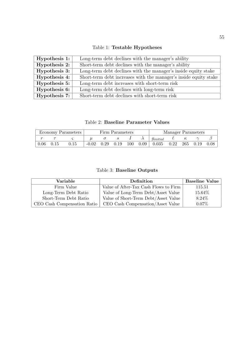
55
Table 1: Testable Hypotheses
Hypothesis 1: Long-term debt declines with the manager’s abilityHypothesis 2: Short-term debt declines with the manager’s abilityHypothesis 3: Long-term debt declines with the manager’s inside equity stakeHypothesis 4: Short-term debt increases with the manager’s inside equity stakeHypothesis 5: Long-term debt increases with short-term riskHypothesis 6: Long-term debt declines with long-term riskHypothesis 7: Short-term debt declines with short-term risk
Table 2: Baseline Parameter Values
Economy Parameters Firm Parameters Manager Parameters
r τ ς µ σ s I λ ginitial ℓ κ γ β
0.06 0.15 0.15 -0.02 0.29 0.19 100 0.09 0.035 0.22 265 0.19 0.08
Table 3: Baseline Outputs
Variable Definition Baseline Value
Firm Value Value of After-Tax Cash Flows to Firm 115.51Long-Term Debt Ratio Value of Long-Term Debt/Asset Value 15.64%Short-Term Debt Ratio Value of Short-Term Debt/Asset Value 8.24%
CEO Cash Compensation Ratio CEO Cash Compensation/Asset Value 0.07%
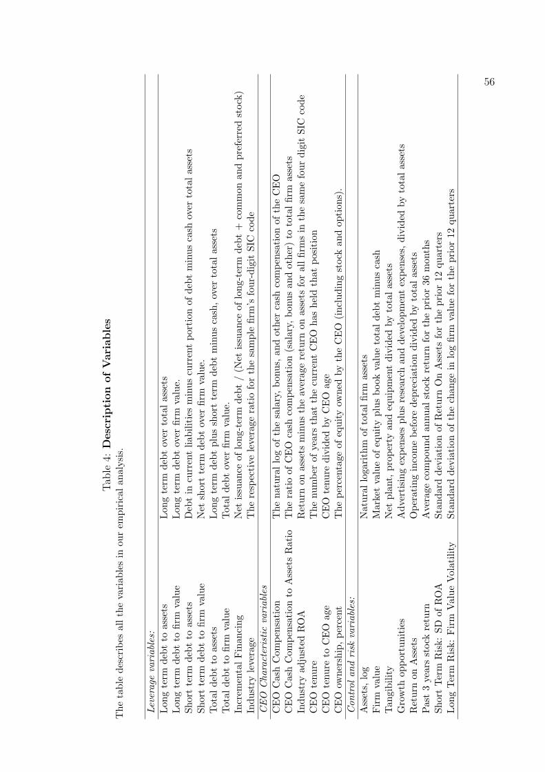
56
Tab
le4:
DescriptionofVariables
Thetable
describes
allthevariab
lesin
ourem
pirical
analysis.
Leverage
variables:
Lon
gterm
debtto
assets
Lon
gterm
debtover
totalassets
Lon
gterm
debtto
firm
value
Lon
gterm
debtover
firm
value.
Shortterm
debtto
assets
Debtin
currentliabilitiesminuscurrentportionofdebtminuscash
over
totalassets
Shortterm
debtto
firm
value
Net
shortterm
debtover
firm
value.
Total
deb
tto
assets
Lon
gterm
debtplusshort
term
debtminuscash,over
totalassets
Total
deb
tto
firm
value
Total
debtover
firm
value.
Increm
entalFinan
cing
Net
issuan
ceoflong-term
debt/(N
etissuance
oflong-term
debt+
common
andpreferred
stock)
Industry
leverag
eTherespectiveleverageratioforthesample
firm
’sfour-digitSIC
code
CEO
Characteristicvariables
CEO
CashCom
pensation
Thenaturallogofthesalary,bonus,
andother
cash
compensationoftheCEO
CEO
CashCom
pensation
toAssetsRatio
Theratioof
CEO
cash
compensation(salary,bonusandother)to
totalfirm
assets
Industry
adjusted
ROA
Return
onassetsminustheaveragereturn
onassetsforallfirm
sin
thesamefourdigit
SIC
code
CEO
tenure
Thenumber
ofyears
thatthecurrentCEO
hasheldthatposition
CEO
tenure
toCEO
age
CEO
tenure
divided
byCEO
age
CEO
ownership,percent
Thepercentageofequityow
ned
bytheCEO
(includingstock
andoption
s).
Controlandrisk
variables:
Assets,
log
Naturalloga
rithm
oftotalfirm
assets
Firm
value
Market
valueofequityplusbookvaluetotaldebtminuscash
Tan
gibility
Net
plant,property
andequipmentdivided
bytotalassets
Growth
opportunities
Advertisingexpensesplusresearchanddevelopmentexpenses,
divided
bytotalassets
Return
onAssets
Operatingincomebefore
depreciationdivided
bytotalassets
Past3years
stock
return
Averag
ecompoundannualstock
return
fortheprior36months
ShortTerm
Risk:SD
ofROA
StandarddeviationofReturn
OnAssetsfortheprior12quarters
Lon
gTerm
Risk:Firm
ValueVolatility
Standarddeviationofthechangein
logfirm
valuefortheprior12quarters
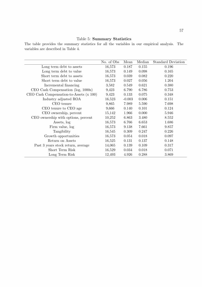
57
Table 5: Summary StatisticsThe table provides the summary statistics for all the variables in our empirical analysis. The
variables are described in Table 4.
No. of Obs Mean Median Standard Deviation
Long term debt to assets 16,573 0.187 0.155 0.196Long term debt to value 16,573 0.149 0.098 0.165Short term debt to assets 16,573 0.039 0.082 0.220Short term debt to value 16,573 0.027 0.056 1.204Incremental financing 3,582 0.549 0.621 0.380
CEO Cash Compensation (log, 1000s) 9,423 6.790 6.786 0.753CEO Cash Compensation-to-Assets (x 100) 9,423 0.133 0.075 0.348
Industry adjusted ROA 16,523 -0.003 0.006 0.151CEO tenure 9,865 7.989 5.590 7.698
CEO tenure to CEO age 9,666 0.140 0.101 0.124CEO ownership, percent 15,142 1.966 0.000 5.946
CEO ownership with options, percent 10,252 6.863 3.480 8.552Assets, log 16,573 6.766 6.653 1.686
Firm value, log 16,573 9.138 7.661 9.857Tangibility 16,545 0.309 0.247 0.226
Growth opportunities 16,573 0.054 0.018 0.097Return on Assets 16,525 0.131 0.137 0.148
Past 3 years stock return, average 14,065 0.139 0.109 0.317Short Term Risk 16,529 0.034 0.018 0.071Long Term Risk 12,493 4.926 0.288 3.869
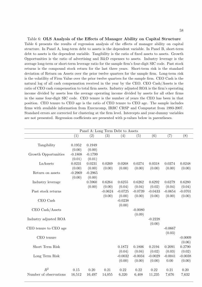
58
Table 6: OLS Analysis of the Effects of Manager Ability on Capital StructureTable 6 presents the results of regression analysis of the effects of manager ability on capital
structure. In Panel A, long-term debt to assets is the dependent variable. In Panel B, short-term
debt to assets is the dependent variable. Tangibility is the ratio of fixed assets to assets. Growth
Opportunities is the ratio of advertising and R&D expenses to assets. Industry leverage is the
average long-term or short-term leverage ratio for the sample firm’s four-digit SIC code. Past stock
returns is the compound stock return for the last three years. Short-term risk is the standard
deviation of Return on Assets over the prior twelve quarters for the sample firm. Long-term risk
is the volatility of Firm Value over the prior twelve quarters for the sample firm. CEO Cash is the
natural log of all cash compensation received in the year by the CEO. CEO Cash/Assets is the
ratio of CEO cash compensation to total firm assets. Industry adjusted ROA is the firm’s operating
income divided by assets less the average operating income divided by assets for all other firms
in the same four-digit SIC code. CEO tenure is the number of years the CEO has been in that
position. CEO tenure to CEO age is the ratio of CEO tenure to CEO age. The sample includes
firms with available information from Execucomp, IRRC CRSP and Compustat from 1993-2007.
Standard errors are corrected for clustering at the firm level. Intercepts and year-dummy variables
are not presented. Regression coefficients are presented with p-values below in parentheses.
Panel A: Long Term Debt to Assets
(1) (2) (3) (4) (5) (6) (7) (8)
Tangibility 0.1952 0.1949(0.00) (0.00)
Growth Opportunities -0.1808 -0.1799(0.01) (0.01)
LnAssets 0.0231 0.0231 0.0269 0.0268 0.0274 0.0318 0.0374 0.0248(0.00) (0.00) (0.00) (0.00) (0.00) (0.00) (0.00) (0.00)
Return on assets -0.2969 -0.2965(0.00) (0.00)
Industry leverage 0.5960 0.6264 0.6255 0.6262 0.6292 0.6279 0.6280(0.00) (0.00) (0.04) (0.04) (0.02) (0.04) (0.04)
Past stock returns -0.0624 -0.0725 -0.0739 -0.0433 -0.0654 -0.0701(0.00) (0.00) (0.00) (0.00) (0.00) (0.00)
CEO Cash -0.0238(0.00)
CEO Cash/Assets -0.0080(0.09)
Industry adjusted ROA -0.2228(0.00)
CEO tenure to CEO age -0.0667(0.03)
CEO tenure -0.0009(0.06)
Short Term Risk 0.1872 0.1806 0.2194 0.2091 0.2790(0.04) (0.04) (0.02) (0.03) (0.02)
Long Term Risk -0.0032 -0.0034 -0.0029 -0.0041 -0.0038(0.00) (0.00) (0.00) 0.00 (0.00)
R2 0.15 0.20 0.21 0.22 0.22 0.22 0.21 0.20Number of observations 16,512 16,497 14,055 6,320 6,408 11,235 7,676 7,632

59
Panel B: Short Term Debt to Assets
(1) (2) (3) (4) (5) (6) (7) (8)
Tangibility 0.0948 0.0939(0.00) (0.00)
Growth Opportunities -0.4779 -0.4654(0.00) (0.00)
LnAssets 0.0238 0.0237 0.0345 0.0210 0.0217 0.0270 0.0136 0.0212(0.00) (0.00) (0.00) (0.00) (0.00) (0.00) (0.00) (0.00)
Return on assets 0.0963 0.0968(0.06) (0.06)
Industry leverage 0.7267 0.7345 0.0300 0.0306 0.0293 0.0309 0.0320(0.00) (0.00) (0.03) (0.03) (0.13) (0.03) (0.03)
Past stock returns -0.0034 -0.0640 -0.0662 -0.0729 -0.0781 -0.0663(0.00) (0.00) (0.00) (0.00) (0.00) (0.00)
CEO Cash -0.0332(0.00)
CEO Cash/Assets -0.0034(0.04)
Industry adjusted ROA -0.2180(0.01)
CEO tenure to CEO age -0.1675(0.00)
CEO tenure -0.0022(0.00)
Short Term Risk -0.1236 -0.1232 -0.4223 -0.1184 -0.1164(0.00) (0.00) (0.03) (0.00) (0.00)
Long Term Risk -0.0047 -0.0051 -0.0083 -0.0053 -0.0054(0.00) (0.00) (0.00) (0.00) (0.01)
R2 0.15 0.16 0.29 0.24 0.24 0.23 0.24 0.23Number of observations 16,512 16,494 14,053 6,346 6,434 11,310 6,817 6,777
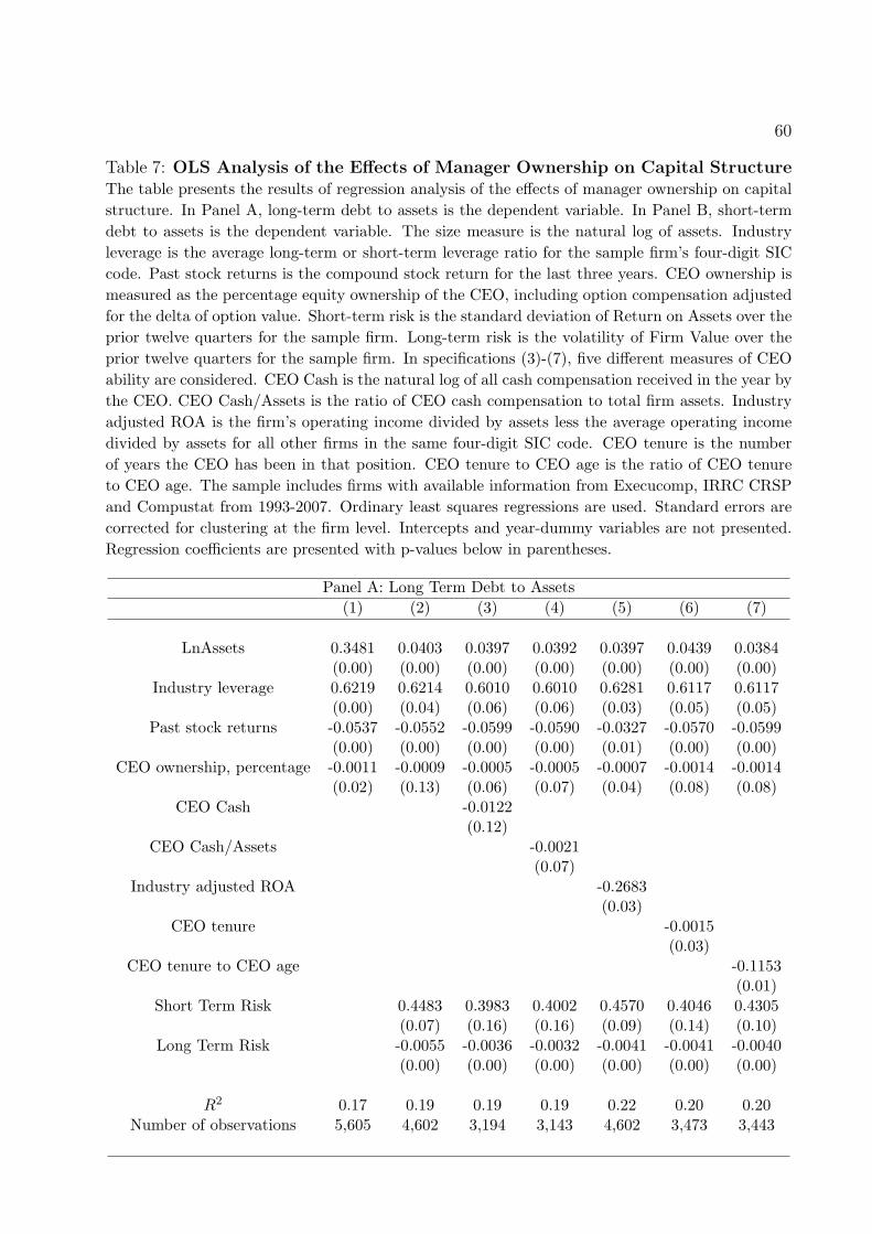
60
Table 7: OLS Analysis of the Effects of Manager Ownership on Capital StructureThe table presents the results of regression analysis of the effects of manager ownership on capital
structure. In Panel A, long-term debt to assets is the dependent variable. In Panel B, short-term
debt to assets is the dependent variable. The size measure is the natural log of assets. Industry
leverage is the average long-term or short-term leverage ratio for the sample firm’s four-digit SIC
code. Past stock returns is the compound stock return for the last three years. CEO ownership is
measured as the percentage equity ownership of the CEO, including option compensation adjusted
for the delta of option value. Short-term risk is the standard deviation of Return on Assets over the
prior twelve quarters for the sample firm. Long-term risk is the volatility of Firm Value over the
prior twelve quarters for the sample firm. In specifications (3)-(7), five different measures of CEO
ability are considered. CEO Cash is the natural log of all cash compensation received in the year by
the CEO. CEO Cash/Assets is the ratio of CEO cash compensation to total firm assets. Industry
adjusted ROA is the firm’s operating income divided by assets less the average operating income
divided by assets for all other firms in the same four-digit SIC code. CEO tenure is the number
of years the CEO has been in that position. CEO tenure to CEO age is the ratio of CEO tenure
to CEO age. The sample includes firms with available information from Execucomp, IRRC CRSP
and Compustat from 1993-2007. Ordinary least squares regressions are used. Standard errors are
corrected for clustering at the firm level. Intercepts and year-dummy variables are not presented.
Regression coefficients are presented with p-values below in parentheses.
Panel A: Long Term Debt to Assets
(1) (2) (3) (4) (5) (6) (7)
LnAssets 0.3481 0.0403 0.0397 0.0392 0.0397 0.0439 0.0384(0.00) (0.00) (0.00) (0.00) (0.00) (0.00) (0.00)
Industry leverage 0.6219 0.6214 0.6010 0.6010 0.6281 0.6117 0.6117(0.00) (0.04) (0.06) (0.06) (0.03) (0.05) (0.05)
Past stock returns -0.0537 -0.0552 -0.0599 -0.0590 -0.0327 -0.0570 -0.0599(0.00) (0.00) (0.00) (0.00) (0.01) (0.00) (0.00)
CEO ownership, percentage -0.0011 -0.0009 -0.0005 -0.0005 -0.0007 -0.0014 -0.0014(0.02) (0.13) (0.06) (0.07) (0.04) (0.08) (0.08)
CEO Cash -0.0122(0.12)
CEO Cash/Assets -0.0021(0.07)
Industry adjusted ROA -0.2683(0.03)
CEO tenure -0.0015(0.03)
CEO tenure to CEO age -0.1153(0.01)
Short Term Risk 0.4483 0.3983 0.4002 0.4570 0.4046 0.4305(0.07) (0.16) (0.16) (0.09) (0.14) (0.10)
Long Term Risk -0.0055 -0.0036 -0.0032 -0.0041 -0.0041 -0.0040(0.00) (0.00) (0.00) (0.00) (0.00) (0.00)
R2 0.17 0.19 0.19 0.19 0.22 0.20 0.20Number of observations 5,605 4,602 3,194 3,143 4,602 3,473 3,443

61
Panel B: Short Term Debt to Assets
(1) (2) (3) (4) (5) (6) (7)
LnAssets 0.0407 0.0297 0.0287 0.0288 0.0301 0.0193 0.0288(0.00) (0.00) (0.00) (0.00) (0.00) (0.00) (0.00)
Industry leverage 0.5407 0.5519 0.5316 0.5309 0.5449 0.5302 0.5361(0.00) (0.03) (0.04) (0.04) (0.04) (0.04) (0.04)
Past stock returns -0.0346 -0.0545 -0.0717 -0.0699 -0.0684 -0.0835 -0.0723(0.00) (0.00) (0.00) (0.00) (0.00) (0.00) (0.00)
CEO ownership, percentage -0.0004 -0.0008 -0.0012 -0.0009 -0.0008 -0.0010 -0.0013(0.59) (0.13) (0.12) (0.14) (0.09) (0.09) (0.09)
CEO Cash -0.0369(0.01)
CEO Cash/Assets -0.0105(0.05)
Industry adjusted ROA -0.1658(0.08)
CEO tenure -0.0019(0.02)
CEO tenure to CEO age -0.1544(0.00)
Short Term Risk -0.0852 -0.1186 -0.1189 -0.0610 -0.1130 -0.1161(0.00) (0.00) (0.00) (0.01) (0.02) (0.02)
Long Term Risk -0.0069 -0.0050 -0.0046 -0.0078 -0.0054 -0.0054(0.00) (0.00) (0.00) (0.00) (0.00) (0.01)
R2 0.16 0.18 0.22 0.22 0.19 0.23 0.21Number of observations 5,604 4,601 3,193 3,142 4,601 3,472 3,442
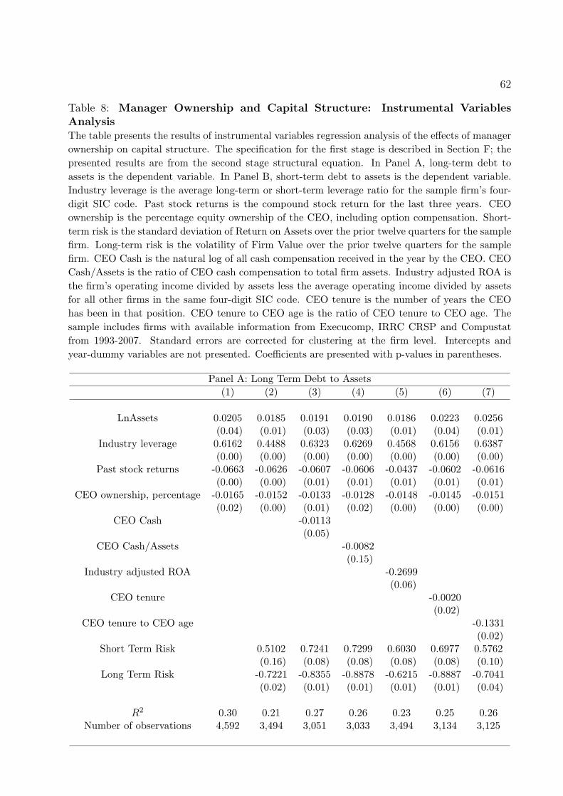
62
Table 8: Manager Ownership and Capital Structure: Instrumental VariablesAnalysisThe table presents the results of instrumental variables regression analysis of the effects of manager
ownership on capital structure. The specification for the first stage is described in Section F; the
presented results are from the second stage structural equation. In Panel A, long-term debt to
assets is the dependent variable. In Panel B, short-term debt to assets is the dependent variable.
Industry leverage is the average long-term or short-term leverage ratio for the sample firm’s four-
digit SIC code. Past stock returns is the compound stock return for the last three years. CEO
ownership is the percentage equity ownership of the CEO, including option compensation. Short-
term risk is the standard deviation of Return on Assets over the prior twelve quarters for the sample
firm. Long-term risk is the volatility of Firm Value over the prior twelve quarters for the sample
firm. CEO Cash is the natural log of all cash compensation received in the year by the CEO. CEO
Cash/Assets is the ratio of CEO cash compensation to total firm assets. Industry adjusted ROA is
the firm’s operating income divided by assets less the average operating income divided by assets
for all other firms in the same four-digit SIC code. CEO tenure is the number of years the CEO
has been in that position. CEO tenure to CEO age is the ratio of CEO tenure to CEO age. The
sample includes firms with available information from Execucomp, IRRC CRSP and Compustat
from 1993-2007. Standard errors are corrected for clustering at the firm level. Intercepts and
year-dummy variables are not presented. Coefficients are presented with p-values in parentheses.
Panel A: Long Term Debt to Assets
(1) (2) (3) (4) (5) (6) (7)
LnAssets 0.0205 0.0185 0.0191 0.0190 0.0186 0.0223 0.0256(0.04) (0.01) (0.03) (0.03) (0.01) (0.04) (0.01)
Industry leverage 0.6162 0.4488 0.6323 0.6269 0.4568 0.6156 0.6387(0.00) (0.00) (0.00) (0.00) (0.00) (0.00) (0.00)
Past stock returns -0.0663 -0.0626 -0.0607 -0.0606 -0.0437 -0.0602 -0.0616(0.00) (0.00) (0.01) (0.01) (0.01) (0.01) (0.01)
CEO ownership, percentage -0.0165 -0.0152 -0.0133 -0.0128 -0.0148 -0.0145 -0.0151(0.02) (0.00) (0.01) (0.02) (0.00) (0.00) (0.00)
CEO Cash -0.0113(0.05)
CEO Cash/Assets -0.0082(0.15)
Industry adjusted ROA -0.2699(0.06)
CEO tenure -0.0020(0.02)
CEO tenure to CEO age -0.1331(0.02)
Short Term Risk 0.5102 0.7241 0.7299 0.6030 0.6977 0.5762(0.16) (0.08) (0.08) (0.08) (0.08) (0.10)
Long Term Risk -0.7221 -0.8355 -0.8878 -0.6215 -0.8887 -0.7041(0.02) (0.01) (0.01) (0.01) (0.01) (0.04)
R2 0.30 0.21 0.27 0.26 0.23 0.25 0.26Number of observations 4,592 3,494 3,051 3,033 3,494 3,134 3,125
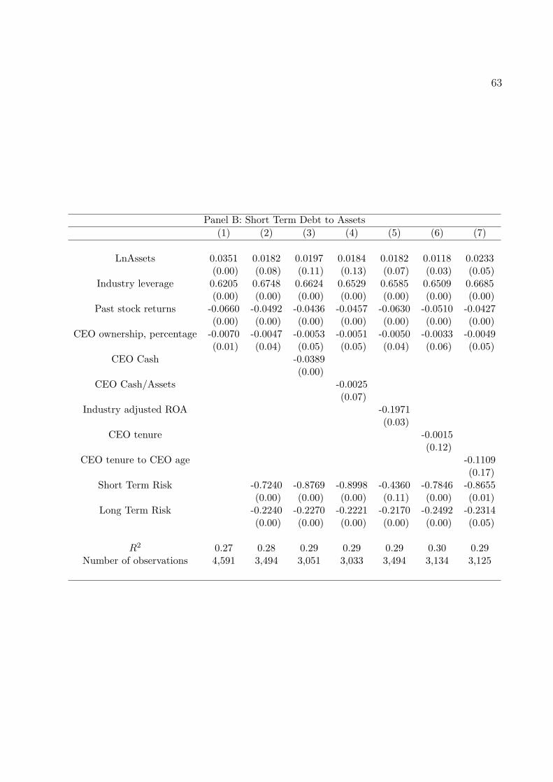
63
Panel B: Short Term Debt to Assets
(1) (2) (3) (4) (5) (6) (7)
LnAssets 0.0351 0.0182 0.0197 0.0184 0.0182 0.0118 0.0233(0.00) (0.08) (0.11) (0.13) (0.07) (0.03) (0.05)
Industry leverage 0.6205 0.6748 0.6624 0.6529 0.6585 0.6509 0.6685(0.00) (0.00) (0.00) (0.00) (0.00) (0.00) (0.00)
Past stock returns -0.0660 -0.0492 -0.0436 -0.0457 -0.0630 -0.0510 -0.0427(0.00) (0.00) (0.00) (0.00) (0.00) (0.00) (0.00)
CEO ownership, percentage -0.0070 -0.0047 -0.0053 -0.0051 -0.0050 -0.0033 -0.0049(0.01) (0.04) (0.05) (0.05) (0.04) (0.06) (0.05)
CEO Cash -0.0389(0.00)
CEO Cash/Assets -0.0025(0.07)
Industry adjusted ROA -0.1971(0.03)
CEO tenure -0.0015(0.12)
CEO tenure to CEO age -0.1109(0.17)
Short Term Risk -0.7240 -0.8769 -0.8998 -0.4360 -0.7846 -0.8655(0.00) (0.00) (0.00) (0.11) (0.00) (0.01)
Long Term Risk -0.2240 -0.2270 -0.2221 -0.2170 -0.2492 -0.2314(0.00) (0.00) (0.00) (0.00) (0.00) (0.05)
R2 0.27 0.28 0.29 0.29 0.29 0.30 0.29Number of observations 4,591 3,494 3,051 3,033 3,494 3,134 3,125
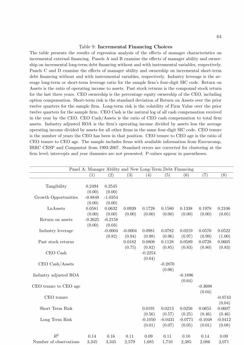
64
Table 9: Incremental Financing ChoicesThe table presents the results of regression analysis of the effects of manager characteristics on
incremental external financing. Panels A and B examine the effects of manager ability and owner-
ship on incremental long-term debt financing without and with instrumental variables, respectively.
Panels C and D examine the effects of manager ability and ownership on incremental short-term
debt financing without and with instrumental variables, respectively. Industry leverage is the av-
erage long-term or short-term leverage ratio for the sample firm’s four-digit SIC code. Return on
Assets is the ratio of operating income to assets. Past stock returns is the compound stock return
for the last three years. CEO ownership is the percentage equity ownership of the CEO, including
option compensation. Short-term risk is the standard deviation of Return on Assets over the prior
twelve quarters for the sample firm. Long-term risk is the volatility of Firm Value over the prior
twelve quarters for the sample firm. CEO Cash is the natural log of all cash compensation received
in the year by the CEO. CEO Cash/Assets is the ratio of CEO cash compensation to total firm
assets. Industry adjusted ROA is the firm’s operating income divided by assets less the average
operating income divided by assets for all other firms in the same four-digit SIC code. CEO tenure
is the number of years the CEO has been in that position. CEO tenure to CEO age is the ratio of
CEO tenure to CEO age. The sample includes firms with available information from Execucomp,
IRRC CRSP and Compustat from 1993-2007. Standard errors are corrected for clustering at the
firm level; intercepts and year dummies are not presented. P-values appear in parentheses.
Panel A: Manager Ability and New Long-Term Debt Financing
(1) (2) (3) (4) (5) (6) (7) (8)
Tangibility 0.2494 0.2545(0.00) (0.00)
Growth Opportunities -0.8848 -1.0354(0.00) (0.00)
LnAssets 0.0581 0.0632 0.0939 0.1728 0.1580 0.1338 0.1978 0.2106(0.00) (0.00) (0.00) (0.00) (0.00) (0.00) (0.00) (0.05)
Return on assets -0.2625 -0.2158(0.00) (0.03)
Industry leverage -0.0004 -0.0004 0.0981 0.0782 0.0219 0.0570 0.0522(0.82) (0.94) (0.98) (0.96) (0.97) (0.99) (1.00)
Past stock returns 0.0182 0.0808 0.1128 0.0589 0.0728 0.0605(0.75) (0.82) (0.85) (0.83) (0.80) (0.83)
CEO Cash -0.2254(0.04)
CEO Cash/Assets -0.2870(0.06)
Industry adjusted ROA -0.1896(0.64)
CEO tenure to CEO age -0.3698(0.04)
CEO tenure -0.0743(0.04)
Short Term Risk 0.0191 0.0213 0.0256 0.0655 0.0607(0.56) (0.57) (0.25) (0.46) (0.46)
Long Term Risk -0.1050 -0.0431 -0.0771 -0.1048 -0.0412(0.01) (0.07) (0.05) (0.01) (0.08)
R2 0.14 0.16 0.11 0.09 0.11 0.10 0.14 0.09Number of observations 3,345 3,345 2,579 1,685 1,710 2,385 2,086 2,071

65
Panel B: Manager Ability and New Long-Term Debt Financing: IV Analysis
(1) (2) (3) (4) (5) (6) (7)
LnAssets 0.0834 0.2312 0.2419 0.2254 0.2941 0.3014 0.3511(0.00) (0.02) (0.04) (0.10) (0.03) (0.09) (0.10)
Industry leverage 0.3812 0.7475 0.7146 0.7297 0.8922 1.0136 1.0527(0.04) (0.00) (0.00) (0.02) (0.09) (0.01) (0.05)
Past stock returns -0.0118 0.1487 0.1202 0.1691 0.2022 0.1605 0.2628(0.91) (0.06) (0.05) (0.05) (0.03) (0.04) (0.05)
CEO ownership, percentage -0.0220 -0.0321 -0.1816 -0.1180 -0.1767 -0.2226 -0.2264(0.02) (0.04) (0.08) (0.04) (0.09) (0.00) (0.05)
CEO Cash -0.0500(0.01)
CEO Cash/Assets -0.1030(0.01)
Industry adjusted ROA -0.0207(0.09)
CEO tenure -0.1063(0.09)
CEO tenure to CEO age -0.0719(0.01)
Short Term Risk 0.0989 0.0905 0.1180 0.1367 0.1656 0.2291(0.01) (0.08) (0.03) (0.08) (0.08) (0.10)
Long Term Risk -0.1526 -0.0554 -0.1239 -0.2082 -0.0436 -0.0734(0.16) (0.06) (0.01) (0.16) (0.12) (0.01)
R2 0.14 0.13 0.13 0.10 0.13 0.16 0.16Number of observations 2,501 1,169 1,101 1,087 1,168 1,189 1,166
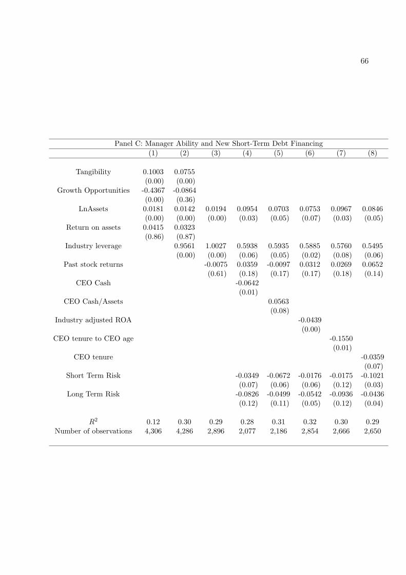
66
Panel C: Manager Ability and New Short-Term Debt Financing
(1) (2) (3) (4) (5) (6) (7) (8)
Tangibility 0.1003 0.0755(0.00) (0.00)
Growth Opportunities -0.4367 -0.0864(0.00) (0.36)
LnAssets 0.0181 0.0142 0.0194 0.0954 0.0703 0.0753 0.0967 0.0846(0.00) (0.00) (0.00) (0.03) (0.05) (0.07) (0.03) (0.05)
Return on assets 0.0415 0.0323(0.86) (0.87)
Industry leverage 0.9561 1.0027 0.5938 0.5935 0.5885 0.5760 0.5495(0.00) (0.00) (0.06) (0.05) (0.02) (0.08) (0.06)
Past stock returns -0.0075 0.0359 -0.0097 0.0312 0.0269 0.0652(0.61) (0.18) (0.17) (0.17) (0.18) (0.14)
CEO Cash -0.0642(0.01)
CEO Cash/Assets 0.0563(0.08)
Industry adjusted ROA -0.0439(0.00)
CEO tenure to CEO age -0.1550(0.01)
CEO tenure -0.0359(0.07)
Short Term Risk -0.0349 -0.0672 -0.0176 -0.0175 -0.1021(0.07) (0.06) (0.06) (0.12) (0.03)
Long Term Risk -0.0826 -0.0499 -0.0542 -0.0936 -0.0436(0.12) (0.11) (0.05) (0.12) (0.04)
R2 0.12 0.30 0.29 0.28 0.31 0.32 0.30 0.29Number of observations 4,306 4,286 2,896 2,077 2,186 2,854 2,666 2,650
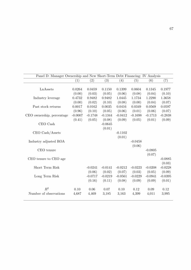
67
Panel D: Manager Ownership and New Short-Term Debt Financing: IV Analysis
(1) (2) (3) (4) (5) (6) (7)
LnAssets 0.0264 0.0459 0.1150 0.1399 0.0604 0.1345 0.1977(0.00) (0.03) (0.05) (0.06) (0.08) (0.04) (0.10)
Industry leverage 0.4732 0.9482 0.9482 1.0445 1.1734 1.2290 1.3658(0.00) (0.02) (0.10) (0.08) (0.00) (0.04) (0.07)
Past stock returns 0.0017 0.0162 0.0035 0.0416 0.0349 0.0569 0.0597(0.96) (0.10) (0.05) (0.06) (0.01) (0.06) (0.07)
CEO ownership, percentage -0.0007 -0.1748 -0.1344 -0.0412 -0.1698 -0.1713 -0.2838(0.41) (0.05) (0.08) (0.09) (0.05) (0.01) (0.09)
CEO Cash -0.0645(0.01)
CEO Cash/Assets -0.1102(0.01)
Industry adjusted ROA -0.0458(0.06)
CEO tenure -0.0805(0.07)
CEO tenure to CEO age -0.0885(0.03)
Short Term Risk -0.0241 -0.0141 -0.0212 -0.0223 -0.0208 -0.0228(0.06) (0.02) (0.07) (0.03) (0.05) (0.09)
Long Term Risk -0.0717 -0.0219 -0.0561 -0.0229 -0.0941 -0.0395(0.16) (0.11) (0.08) (0.09) (0.09) (0.01)
R2 0.10 0.06 0.07 0.10 0.12 0.09 0.12Number of observations 4,687 4,469 3,185 3,163 4,399 4,011 3,995
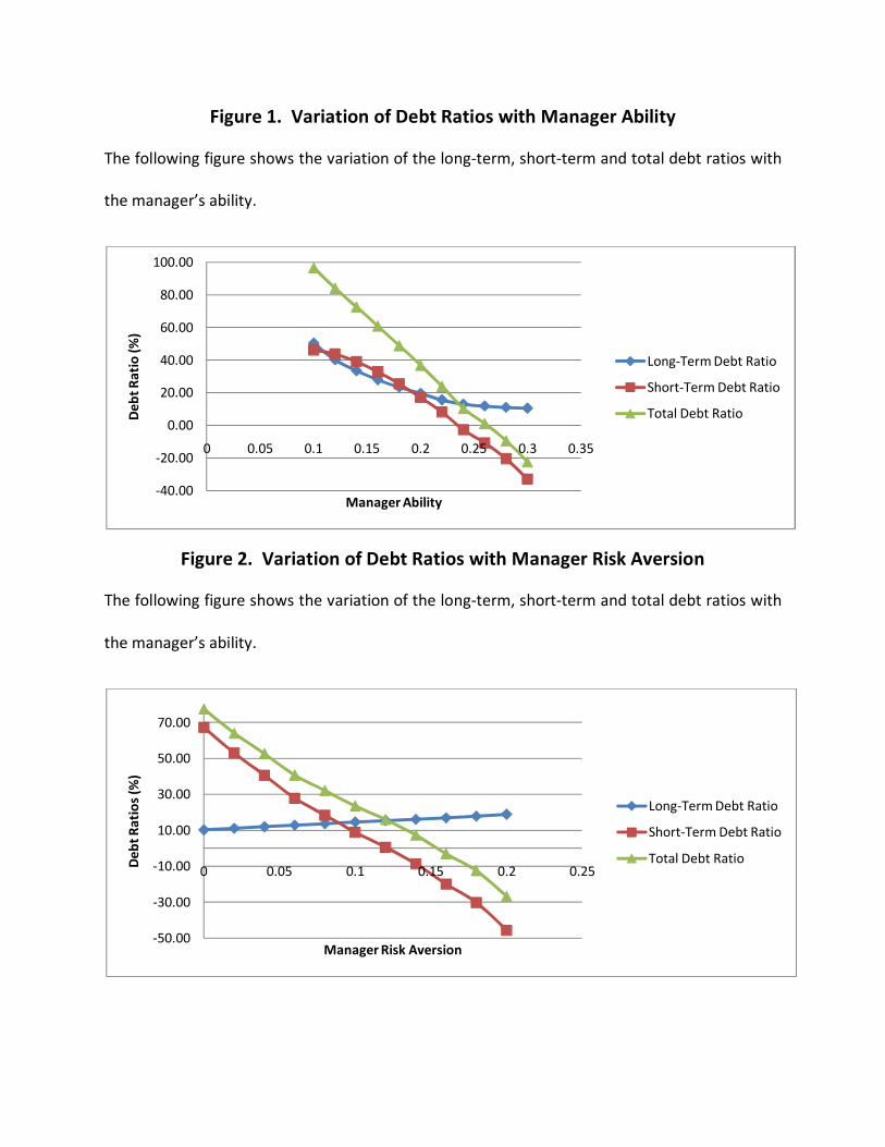
Figure 1. Variation of Debt Ratios with Manager Ability
The following figure shows the variation of the long-term, short-term and total debt ratios with
the manager’s ability.
Figure 2. Variation of Debt Ratios with Manager Risk Aversion
The following figure shows the variation of the long-term, short-term and total debt ratios with
the manager’s ability.
-40.00
-20.00
0.00
20.00
40.00
60.00
80.00
100.00
0 0.05 0.1 0.15 0.2 0.25 0.3 0.35
De
bt
Ra
tio
(%
)
Manager Ability
Long-Term Debt Ratio
Short-Term Debt Ratio
Total Debt Ratio
-50.00
-30.00
-10.00
10.00
30.00
50.00
70.00
0 0.05 0.1 0.15 0.2 0.25
De
bt
Ra
tio
s (%
)
Manager Risk Aversion
Long-Term Debt Ratio
Short-Term Debt Ratio
Total Debt Ratio
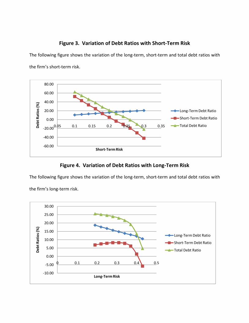
Figure 3. Variation of Debt Ratios with Short-Term Risk
The following figure shows the variation of the long-term, short-term and total debt ratios with
the firm’s short-term risk.
Figure 4. Variation of Debt Ratios with Long-Term Risk
The following figure shows the variation of the long-term, short-term and total debt ratios with
the firm’s long-term risk.
-60.00
-40.00
-20.00
0.00
20.00
40.00
60.00
80.00
0.05 0.1 0.15 0.2 0.25 0.3 0.35De
bt
Ra
tio
s (%
)
Short-Term Risk
Long-Term Debt Ratio
Short-Term Debt Ratio
Total Debt Ratio
-10.00
-5.00
0.00
5.00
10.00
15.00
20.00
25.00
30.00
0 0.1 0.2 0.3 0.4 0.5
De
bt
Ra
tio
s (%
)
Long-Term Risk
Long-Term Debt Ratio
Short-Term Debt Ratio
Total Debt Ratio

Figure 5. Variation of Debt Ratios with Manager’s Initial Stake
The following figure shows the variation of the long-term, short-term and total debt ratios with
the manager’s initial ownership stake.
Figure 6. Effects of Manager’s Bargaining Power on Long-Term Debt
The following figure shows the effects of the manager’s bargaining power on the variation of
the long-term debt ratio with the manager’s ability.
-5.00
0.00
5.00
10.00
15.00
20.00
25.00
30.00
0 0.02 0.04 0.06 0.08
De
bt
Ra
tio
s (%
)
Manager's Initial Stake
Long-Term Debt Ratio
Short-Term Debt Ratio
Total Debt Ratio
0.00
10.00
20.00
30.00
40.00
50.00
60.00
70.00
0 0.05 0.1 0.15 0.2 0.25 0.3 0.35
Lon
g-T
erm
De
bt
Ra
tio
(%
)
Manager Ability
omega = 0.2
omega = 0.4
omega = 0.6
omega = 0.8
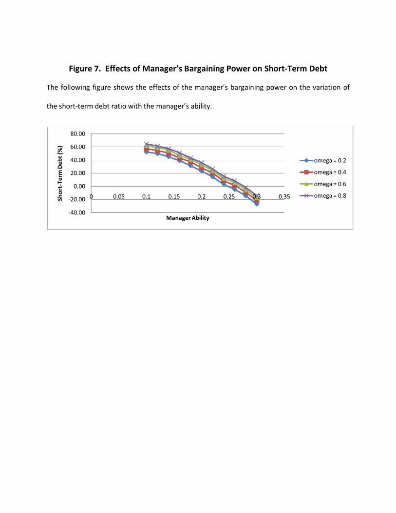
Figure 7. Effects of Manager’s Bargaining Power on Short-Term Debt
The following figure shows the effects of the manager’s bargaining power on the variation of
the short-term debt ratio with the manager’s ability.
-40.00
-20.00
0.00
20.00
40.00
60.00
80.00
0 0.05 0.1 0.15 0.2 0.25 0.3 0.35Sh
ort
-Te
rm D
eb
t (%
)
Manager Ability
omega = 0.2
omega = 0.4
omega = 0.6
omega = 0.8