Common Agricultural Policy Regional Impact – The Rural Development Dimension

Collaborative project - Small to medium-scale focused research project under the Seventh Framework Programme

Project No.: 226195

WP4 Baseline

Deliverable: D4.8

Management guidelines for the CAPRI

baseline

Mihaly HIMICS, Pavel CIAIAN, Benjamin VAN DOORSLAER, Guna SALPUTRA

Partner(s): JRC-IPTS

Final version: 22.02.2013

The views expressed are purely those of the authors and may not in any circumstances be regarded

as stating an official position of the European Commission.

The FP7 project "Common Agricultural Policy Regional Impact – The Rural Development Dimension"

(CAPRI-RD) aims at developing and applying an operational, Pan-European tool including all

Candidate and Potential Candidate countries to analyse the regional impacts of all policy measures

under CAP Pillar I and II across a wide range of economic, social and environmental indicators. The

project is carried out by a consortium of 10 research organisations, led by Bonn University (UBO).

Authors of this report and contact details

Names: Mihály HIMICS, Pavel CIAIAN, Benjamin VAN DOORSLAER,

Guna SALPUTRA

Partner acronym: JRC-IPTS

Address: European Commission - Joint Research Centre (JRC)

Institute for Prospective Technological Studies (IPTS)

Edificio Expo, C/ Inca Garcilaso 3, E-41092 Sevilla, Spain

E-mail: pavel.ciaian@ec.europa.eu

Deliverable 4.8

Page 3 of 32

Table of contents

ABBREVIATIONS ...................................................................................................... 5

1. INTRODUCTION ................................................................................................. 6

2. OVERVIEW OF THE CAPRI MODELLING SYSTEM ......................................... 7

3. CAPRI BUILDING BLOCKS ............................................................................... 9

4. BUILDING A CONSISTENT DATASET FROM DIVERSE STATISTICAL

SOURCES ................................................................................................................ 11

5. BASELINE PROCESS OF DG AGRI ................................................................ 13

6. PROJECTIONS OF THE FUTURE STATE OF THE ECONOMY ..................... 15

6.1. CAPTRD ................................................................................................................................................ 15

6.2. Projections of global commodity balances .......................................................................................... 16

7. CALIBRATION OF THE CAPRI MODELLING SYSTEM ................................. 18

8. VALIDATION OF THE CAPRI BASELINE RESULTS...................................... 20

9. GOOD MANAGEMENT PRACTICES FOR THE BASELINE ........................... 21

10. CONCLUDING REMARKS ........................................................................... 22

REFERENCES ......................................................................................................... 25

ANNEX 1: CALIBRATION STEPS .......................................................................... 27

Deliverable 4.8

Page 5 of 32

Abbreviations

AGLINK- COSIMO

Recursive-dynamic, Partial Equilibrium, Supply Demand Model of World Agriculture, Developed by the OECD Secretariat in Close Co-operation with Member Countries and Certain Non Member Economies

AGMEMOD Agricultural Member State Modelling for the EU and Eastern European Countries

AMAD Agricultural Market Access Database CAP Common Agricultural Policy CAPRI Common Agricultural Policy Regional Impact cif Cost, Insurance and Freight CLC Corine Land Cover COMEXT Intra- and extra-EU Trade Data COSIMO Commodity Simulation Model DG-AGRI Directorate General for Agriculture and Rural Development EAA Economic Accounts for Agriculture EBB European Biodiesel Board ePURE European renewable ethanol ESIM European Simulation Model FAO Food and Agriculture Organization FAOSTAT Statistics Division of the FAO FAPRI Food and Agricultural Policy Research Institute fob Free on Board FSS Farm Structure Survey GDP Gross Domestic Product GLOBIOM Global Model for Assessment of Competition for Land Use between

Agriculture, Bioenergy, and Forestry

GTAP Global Trade Analysis Project GUI Graphical User Interface HPD Bayesian Highest Posterior Density IIASA International Institute for Applied System Analysis IFPRI International Food Policy Research Institute IMPACT International Model for Policy Analysis of Agricultural Commodities

and Trade JRC Joint Research Centre JRC-IPTS Joint Research Centre - Institute for Prospective Technological

Studies NMS New Member States NUTS Nomenclature of Units For Territorial Statistics OECD Organisation for Economic Co-operation and Development PCE Private consumption expenditure deflator PRIMES EU-wide Energy Model UN United Nations USDA United States Department of Agriculture US United States

Deliverable 4.8

Page 6 of 32

1. Introduction

The CAPRI modelling system is designed for comparative static analysis. In its

essence it means comparing alternative scenarios to a given baseline. Constructing

a baseline, therefore, is an integral part of any policy impact analysis with CAPRI.

Building a baseline involves two major steps:

(1) A possible future state of the (global) economy needs to be projected and

translated into a set of consistent model parameters. This also includes

projected values for model-endogenous variables.

(2) The modelling system needs to be calibrated to the projection, i.e. the model

reproduces the above set of projections including of course the endogenous

model variables.

The CAPRI modelling system consists of several interlinked sub-modules that might

follow different calibration approaches. The supply and demand equations of the

global market model, for example, are calibrated by (1) shifting them to projected

levels and (2) trimming the elasticities by using econometric estimations and

imposing regulatory conditions. The regional supply module on the other hand is

calibrated following Positive Mathematical Programming (PMP) techniques, first

formulated by Howitt (Howitt 1995) and has been further improved over the last

decade (Heckelei and Britz 2005).

This report guides the reader through the CAPRI modelling system in order to

complete the two steps from above. The text always refers to the relevant code

implementation in order to give the reader further insights and to help him putting

theory into practice. But given the size of CAPRI this objective can only be fulfilled to

a limited extent and only with the aim of giving the reader a good starting point for his

own further investigation.

Deliverable 4.8

Page 7 of 32

2. Overview of the CAPRI modelling system

CAPRI is a comparative static partial equilibrium model for the agricultural sector

developed for policy and market impact assessments from global to regional and

even farm type scale. It consists of two main components: a set of mathematical

programming models covering the agricultural supply of most European countries

(hereinafter referred to as the 'supply module') and a global equilibrium model for

agricultural commodity markets (hereinafter referred to as the 'market module').

(Figure 1) (Britz and Witzke, 2012).

The market module is a comparative-static, deterministic, partial, spatial, global

equilibrium model covering about 75 countries or country aggregates. Based on the

Armington approach (Armington, 1969), products are differentiated by origin,

enabling to capture bilateral trade flows. The EU is split in three trading blocks:

EU15, EU10 and BUR1). EU trade relations are simulated at this geographical

aggregation level. On the other hand, each of the EU Member States has an own

system of behavioural functions, i.e. supply and demand functions (Britz and Witzke,

2012). The market module is defined by a system of behavioural equations

representing agricultural supply, human consumption, multilateral trade relations,

feeding balances and the processing industry; all differentiated by commodity and

geographical units.

The supply module is composed of separate, regional and farm-type, non-linear

programming models. The regional programming models are based on a model

template assuming profit-maximizing behaviour under technological constraints, most

importantly in animal feeding and fertilizer use, but also constraints on inputs and

outputs such as young animal, land balances and policies (e.g. set-aside) (Jansson

and Heckelei, 2011). The supply module currently covers all individual Member

States of the EU-27 and also Norway, Turkey and the Western Balkans broken down

to about 280 administrative regions (NUTS 2 level) with up to 10 farm-types in each

of the NUTS 2 region (in total 1823 farm-regional models) and more than 50

agricultural products.

The challenge is calibrating these two modules relying on different modelling

paradigms to the same projected state of the economy. The calibration of the market

module requires that market equilibrium conditions are satisfied at calibration point.

The quantities of demand and supply functions are dependent on prices and both

quantities and prices represent the point to which market module is calibrated. On

1 BUR includes Bulgaria and Romania, the two new Member States joined in 2007

Deliverable 4.8

Page 8 of 32

the other hand, the regional programming models in the supply module should be

calibrated to the projected land use and animal production at the same prices the

market module is calibrated to. The calibration requires that first order optimality

conditions (marginal revenues equal to marginal costs, all constraints feasible) hold

in the calibration point for each of the NUTS 2 or farm-type models. Positive

Mathematical Programming (PMP) is applied to close the difference between

marginal revenues and marginal costs in the calibration point by introducing non-

linear terms in the objective function to capture other unaccounted costs (e.g. labour,

capital) such that optimality conditions are satisfied at defined levels of decision

variables (Britz and Witzke 2012).

Figure 1: Structure of CAPRI model

Source: Britz and Witzke (2012)

Deliverable 4.8

Page 9 of 32

3. CAPRI building blocks

Calibration of CAPRI is split in several tools consistently interlinked between them

with the aim to facilitate data manipulation, generation of projections of the future

state of agricultural economy, calibration to the AGLINK-COSIMO baseline and

exploitation of results. The building bocks of CAPRI relevant for the calibration

process can be split in four tools: (1) database tool, (2) projections, (3) calibration

and scenario simulations, and (4) exploitation of results. The interlinkage between

these tools and their specific components are depicted in Figure 2. The main

database tools include MS level database CoCo, regional database CAPREG, and

global database for world regions. CoCo and CAPREG databases alongside other

support data (primarily coming from AGLINK-COSIMO and PRIMES) are key inputs

into the trend projection module (CAPTRD). Calibration is done within the CAPMOD

module combining information from CAPTRD, global database, and policy data. User

friendly results are provided primarily through the Graphical User Interface (GUI) in

form of tables, maps and graphs.

Deliverable 4.8

Page 10 of 32

Figure 2: Interlinkages between CAPRI tools

Calibration and

scenario simulations

Projections Database tool

CoCo MS data

Global World data

CAPREG Regional data Input allocation

DATA Eurostat,

FAO, FADN, etc.

CAPTRD Trend projections

CAPMOD

Support AGLINK,

PRIMES, etc.

Exploitation of results

Tables Maps Graphs

Policies

Deliverable 4.8

Page 11 of 32

4. Building a consistent dataset from diverse statistical sources

A key process necessary to be conducted prior to the baseline work includes

preparation and construction of data. Following the CAPRI structure, the main tools

needed for the baseline construction are:

1. COCO

2. CAPREG

3. Global

4. Policy data (policy module including CAP, trade policies, biofuel mandates

etc.)

The most important source of information for CoCo is EUROSTAT. This in itself

creates a consistency in terms of data definitions for EU Member states and selected

European countries (which would not be the case using national data sources). Other

supporting data sources include: FADN-based estimations (e.g. costs), expert info,

farm practice books, FAO, etc. For specific sub-modules (e.g. biofuels, GHG-

emission accounting, land-use) additional sources are needed as they cannot be

retrieved from standard statistical sources. For example, data for biofuels are

collected from European Biodiesel Board (EBB), European renewable ethanol

(ePURE), PRIMES model database, FO Licht’s World Ethanol and Biofuels Report,

COMEXT trade data, AGLINK-COSIMO model, etc. The data base for land use is

based on information on land use classes from various sources such as Corine Land

Cover (CLC), Farm Structure Survey (FSS), FAO, etc. For the NMS additional data

are included such as national data, FAO and Eurostat contractor Ariane.2 The use of

various sources for building CoCo is to impose completeness and consistency of the

final database in terms of temporal resolution and coverage of all relevant variables.

However, choice of particular database is done in hierarchical steps by giving

preference to key statistical sources (e.g. Eurostat). If data in the first best source

(e.g. Eurostat) are unavailable, then second best sources are used to fill the gaps for

missing data. To combine the various data sources and to ensure consistency of the

final database, Bayesian Highest Posterior Density (HPD) approach is applied. The

main principle of the HDP is to ensure minimal deviation of the estimated values from

the support data, as constructed from the EUROSTAT and non-EUROSTAT

statistical sources, subject to consistency constraints (e.g. closed market balances,

perfect aggregation from lower to higher regional level) (Britz and Witzke 2012).

2 For more detailed description see Britz and Witzke (2012).

Deliverable 4.8

Page 12 of 32

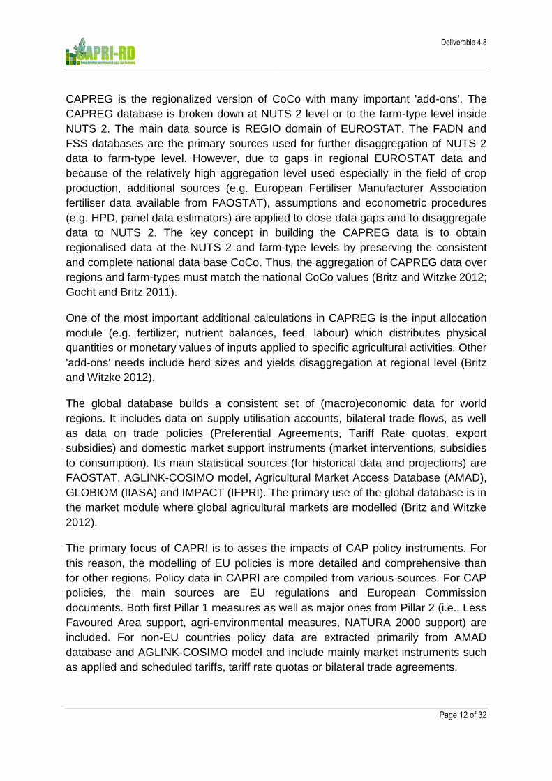
CAPREG is the regionalized version of CoCo with many important 'add-ons'. The

CAPREG database is broken down at NUTS 2 level or to the farm-type level inside

NUTS 2. The main data source is REGIO domain of EUROSTAT. The FADN and

FSS databases are the primary sources used for further disaggregation of NUTS 2

data to farm-type level. However, due to gaps in regional EUROSTAT data and

because of the relatively high aggregation level used especially in the field of crop

production, additional sources (e.g. European Fertiliser Manufacturer Association

fertiliser data available from FAOSTAT), assumptions and econometric procedures

(e.g. HPD, panel data estimators) are applied to close data gaps and to disaggregate

data to NUTS 2. The key concept in building the CAPREG data is to obtain

regionalised data at the NUTS 2 and farm-type levels by preserving the consistent

and complete national data base CoCo. Thus, the aggregation of CAPREG data over

regions and farm-types must match the national CoCo values (Britz and Witzke 2012;

Gocht and Britz 2011).

One of the most important additional calculations in CAPREG is the input allocation

module (e.g. fertilizer, nutrient balances, feed, labour) which distributes physical

quantities or monetary values of inputs applied to specific agricultural activities. Other

'add-ons' needs include herd sizes and yields disaggregation at regional level (Britz

and Witzke 2012).

The global database builds a consistent set of (macro)economic data for world

regions. It includes data on supply utilisation accounts, bilateral trade flows, as well

as data on trade policies (Preferential Agreements, Tariff Rate quotas, export

subsidies) and domestic market support instruments (market interventions, subsidies

to consumption). Its main statistical sources (for historical data and projections) are

FAOSTAT, AGLINK-COSIMO model, Agricultural Market Access Database (AMAD),

GLOBIOM (IIASA) and IMPACT (IFPRI). The primary use of the global database is in

the market module where global agricultural markets are modelled (Britz and Witzke

2012).

The primary focus of CAPRI is to asses the impacts of CAP policy instruments. For

this reason, the modelling of EU policies is more detailed and comprehensive than

for other regions. Policy data in CAPRI are compiled from various sources. For CAP

policies, the main sources are EU regulations and European Commission

documents. Both first Pillar 1 measures as well as major ones from Pillar 2 (i.e., Less

Favoured Area support, agri-environmental measures, NATURA 2000 support) are

included. For non-EU countries policy data are extracted primarily from AMAD

database and AGLINK-COSIMO model and include mainly market instruments such

as applied and scheduled tariffs, tariff rate quotas or bilateral trade agreements.

Deliverable 4.8

Page 13 of 32

5. Baseline process of DG AGRI

DG AGRI annually constructs an outlook for the medium-term developments in

agricultural commodity markets in the EU. This outlook permits a better

understanding of the markets and their dynamics and also contributes to identify key

issues for market and policy developments. Furthermore, the outlook serves as a

benchmark for assessing the medium-term impact of future market and policy issues

(hence we refer to it as ‘baseline’ in the following). The model used for the outlook

projections is a specific version of AGLINK-COSIMO, a recursive dynamic partial

equilibrium model with global coverage. The baseline construction process always

tries to build on the latest available market and policy information. Projection results

are presented in balance sheets for the main agricultural commodities, with detailed

results for the EU. The commodities covered include cereals, oilseeds, sugar, rice,

biofuels, meat and dairy markets (Fellmann and Hélaine 2012).

Figure 3: Flowchart of the baseline construction process

Source: M’barek and Londero (2012)

OECD-FAO Outlook Short-term – DG AGRI

First draft of baseline Macro-economics

Preliminary baseline

Baseline week (discussion with DG AGRI market experts)

Outlook workshop Uncertainty assessment

Calibration-CAPRI

Final baseline Calibration of CAPRI and ESIM

Publication

Deliverable 4.8

Page 14 of 32

The process of the DG AGRI’s baseline construction is depicted in Figure 3.3 The

starting point is the latest available version of the AGLINK-COSIMO model, which

was used for the OECD-FAO Agricultural Outlook4 of that year. The EU module of

AGLINK-COSIMO is then updated and optionally further extended in order to answer

EU-specific research questions (e.g. income module for EU farmers).

An in-depth discussion of the first results takes place between the modelling and

market experts of DG AGRI and the JRC-IPTS during a ‘baseline week’ in

September. After further adjustments, the projections are presented in October at the

‘Commodity Market Development in Europe – Outlook’ workshop, organised by the

DG AGRI and JRC-IPTS. In order to identify and quantify the potential variability of

the market projections, the results of additional scenarios with alternative

assumptions are also presented during the workshop. The workshop gathers high-

level policy makers, modelling and market experts from the EU, the United States

and international organisations such as the FAO, OECD, FAPRI and The World

Bank. The workshop provides a forum to present and discuss recent and projected

developments in the EU agricultural and commodity markets, to outline the reasons

behind observed and prospected developments and to draw conclusions on the

short/medium term prospects of European agricultural markets in the context of world

market developments. Special focus is given to the discussion on the sensitivity of

the projected market developments to different settings/assumptions (regarding for

example macroeconomic uncertainties, biofuel policies, specific drivers of demand

and supply, etc.). Suggestions and comments made during the workshop are taken

into account to improve the final version of the outlook, which is then published in the

report ‘Prospects for Agricultural Markets and Income in the EU’ in December each

year5.

3 More detailed information on the general baseline construction process is given in Nii-Naate (Ed.)

(2011).

4 The OECD-FAO Agricultural Outlook 2012-2021 is available online: http://www.agri-outlook.org/

5 Latest available report can be found here: http://ec.europa.eu/agriculture/markets-and-

prices/reports_en.htm

Deliverable 4.8

Page 15 of 32

6. Projections of the future state of the economy

As mentioned in previous section, CAPRI does not generate its own baseline, but the

main objective is to calibrate it primarily to the DG AGRI baseline generated by

AGLINK-COSIMO model (section 5). However, AGLINK-COSIMO provides baseline

results only at EU15, EU12 and EU27 aggregate level as well as it does not cover a

full set of non-EU regions and activities available in CAPRI. For this reason, CAPRI

needs to supplement AGLINK-COSIMO with internal projections for regional level

and for activities not covered by AGLINK-COSIMO model. At the same time,

projections from other sources (e.g. FAPRI, FAO) are used to supplement AGLINK-

COSIMO data mostly for the non-EU countries.

CAPRI projections are generated in two separate processes: (i) within the trend

projection module (CAPTRD) and (ii) as part of the calibration of market module. The

latter refers to the data balancing problem, aiming at creating consistent commodity

balances at the global scale. The estimation framework in CAPTRD guarantees that

the internal projections are as close as possible to the AGLINK-COSIMO baseline.

The regional supply module is calibrated to the CAPTRD projections. On the other

hand, the market module is calibrated to the outcome of the data balancing problem

of the global commodity markets.

6.1. CAPTRD

CAPTRD (defined in captrd.gms) projects commodity balances and prices for the EU

countries, Norway and Western Balkan (countries covered by the supply module).

Trend projections are derived by minimizing weighted squared deviation of trend

values to support points. The weights reflect the variation of the error terms in the

historical trend model and/or defined by the ‘trust level’ of the supports. The

optimization is subject to a set of consistency constraints. CAPTRD integrates a

multitude of external information sources and historical trends derived from CoCo

and CAPREG. The optimal values can therefore be interpreted as the ‘closest’

consistent projections to a set of external projections/forecasts and historical trends.

More specifically, the a-priori information sources for defining the support points are

typically forecasts and projections from national and international organizations (e.g.

AGLINK-COSIMO baseline, OECD market outlook, EC prospects for commodity

markets). There exists also a built-in possibility in CAPRI to rank the information

sources by their ‘reliability’, the so called ‘trust level’. This involves assigning

appropriate weights to the bits of a-priori information in the constructed Bayesian

Deliverable 4.8

Page 16 of 32

estimator. This issue is highly relevant in applied research (e.g. in policy impact

analysis) because the uncertainty in projecting different model parameters varies to a

great extent. For example, experts might express a high trust with regard to the

outlook on cropping areas at country level, contrary to e.g. the net trade position

which typically shows big variation over time and therefore difficult to predict.

Consistency constraints imposed during the generation of projections link the

different information sources by following some logical rules. Constraints ensure

consistency of projections between different activities and different regional levels. A

simple example is the area balance that links utilized agricultural area and cropping

areas, simply stating that summing up the land use of agricultural activities gives

back total utilized agricultural area. The consistency constraints are fully described in

Britz and Witzke 2012.

Overall the estimation framework in CAPTRD guarantees that projections are as

close as possible to the AGLINK-COSIMO baseline. As AGLINK-COSIMO provides

projection results only at EU15 and EU12 levels, these values are used to scale

proportionally the CAPRI projections at lower aggregation level such that they are

consistent with the AGLINK-COSIMO baseline. These CAPTRD projections are then

used as the targets for the simulation year to which supply module is calibrated.

6.2. Projections of global commodity balances

Projections of global commodity balances, trade and prices for all market regions are

run simultaneously with the calibration (see section 7). Wherever possible, the

AGLINK-COSIMO baseline is used to generate global projections. This is

complemented by other external information sources: Supply and Utilization

Accounts, trade matrices and projections from the FAO; Longer term projections from

GLOBIOM (IIASA) and IMPACT (IFPRI); and biofuel related projections from the

PRIMES energy model. Projections on commodity balances, trade and prices for all

market regions are made consistent simultaneously. Technically, the data balancing

problem is solved by the ‘arm\data_cal.gms’ module.

CAPRI has a separate global data preparation module (global.gms) that collects

information from different sources and converts it to the format accepted by CAPRI

(model specific product definitions, variables etc.). The module constructs a global

database for the base year that serves as the basis of projections until the simulation

year. The database is stored in a set of .gdx containers (under the folder

results\global):

Deliverable 4.8

Page 17 of 32

fao_agg_04.gdx: (1) FAO trade matrices (trade flows) and commodity balances, (2) biofuel-related balances, trade and parameters, (3) technical parameters (elasticities) from the World Food Model

tc_04.gdx: transportation cost estimates, the estimation procedure is integrated in global.gms and is based on the difference between cif and fob prices

tariffs.gdx: applied and bound rates for specific and ad-valorem tariffs, compiled mainly from the AMAD database (aggregated from HS6 level)

f2050_impact.gdx: IMPACT model results mapped to the CAPRI nomenclature

longrun_info_fac.gdx: long-term projections, currently until 2050, compiled from different sources, including PRIMES, IFPRI, FAO, etc.

In a next step, the ‘arm\data_prep.gms’ module collects base year information and growth factors for the market module from various sources and stores it in the parameters DATA and p_growthRateMarketModelPos.

In order to get a consistent quantity and price framework for the market module calibration, a balancing problem for the global commodity markets (market balancing problem) is set up and solved in the ‘arm\data_cal.gms’ module. The balancing problem is defined in ‘arm\cal_models.gms’ and includes the following equations:

Balance identities for market balances, for the two-stage Armington demand system and for trade

Trade policy mechanisms for public intervention, specific and ad-valorem tariffs, tariff rate quotas, export subsidies and the entry price system of fruits and vegetables

Accounting equations along the supply chain, i.e. feeding, processing and biofuel production

Price linkages, i.e. prices derived from the equilibrium market prices (producer, consumer, cif, import and Armington prices); processing margins

The balancing problem is first solved for the base year. Based on the consistent base

year data, prices and quantities are shifted to the simulation year and the balancing

problem is solved again. The algorithm for the balancing problem keeps certain

variables fixed while gradually relaxes others in order to find a feasible solution.

These consistent price and quantity data are then used as the targets for the

simulation year to which market module is finally calibrated.

Deliverable 4.8

Page 18 of 32

7. Calibration of the CAPRI modelling system

As anticipated in section 2, the supply and market modules of CAPRI are

sequentially calibrated in simulation runs (Britz 2008). The calibration of the modules

against the given baseline data generated by CAPTRD and 'arm\data_cal.gms'

therefore requires a consistent calibration point for the supply and market modules

with respect to prices and quantities. However, reflecting the different structure of the

modules, the calibration is based on different principles (PMP approach versus

calibration constraints for a system of equations). The calibration is executed with the

CAPMOD module (Figure 2).6

The supply modules are calibrated following the methods of Positive Mathematical

Programming (PMP), first formulated by Howitt (1995) and improved substantially

over the last decades by addressing the early problems of parameter specification

and simulation behaviour. For a summary on the methodological developments in

PMP modelling, see Heckelei and Britz (2005) and Heckelei, Britz, and Zhang

(2012).

Technically the calibration happens in two consecutive steps both using the

CAPMOD simulation engine in ‘baseline mode’ (Figure 4). First the market model is

calibrated (‘Baseline calibration market model’ in GUI). The data balancing problem

of the commodity markets and the actual calibration of the parameters for the

behavioural equations are solved in one go. Then the supply model is calibrated to

target values including product balances broken down to activity levels, land use,

feed demand and producer prices (‘Baseline calibration supply models’ in GUI). Most

of the target balances are generated by CAPTRD (see section 6.1) while the

producer prices are derived from the same market prices that the market model is

calibrated to.

6 For more detailed hands-on on calibration see Annex 1.

Deliverable 4.8

Page 19 of 32

The communication between CAPTRD and the simulation engine of CAPRI is via a

set of .gdx containers providing the results of the trend projections (in the folder

\results\baseline):

AGLINK_for_capmod.gdx: growth factors for the unit values (prices) in the CAPRI supply modules, derived from AGLINK-COSIMO results

results_0420.gdx: full result set of the trend estimation procedure, including intermediate steps for debugging purposes.

trends_04_20.gdx: trend estimates for the commodity balances and prices (in the simulation year). This is a subset of the full result set stored in results_0420.gdx, containing only the part directly used later by the calibration process

Figure 4: CAPRI GUI with the two consecutive steps of the calibration

The results of the market model calibration are stored under ‘baseline\data_market*year*.gdx’. The unit value prices (UVAG) used in the supply model calibration are prepared in the ‘arm\prep_market.gms’ module and written to disk in the file ‘baseline\data_uvag*year*.gdx’. The internal communication of these prices between supply and market modules are done through the p_pricesInIters parameter.

All calibrated parameters are stored in a single .gdx container ‘results\simini\sim_ini_*geog.level*years*.gdx’. This data file contains all parameters necessary for initiating a simulation run. The .gdx is created with the module ‘capmod\create_sim_ini_gdx.gms’ which calls the data preparation, data balancing and market model calibration modules explained above.

Deliverable 4.8

Page 20 of 32

8. Validation of the CAPRI baseline results

After the calibration of the CAPRI model, the results need to be checked and

validated to ensure reliability and plausibility of the baseline. As CAPRI is calibrated

to the AGLINK-COSIMO baseline, first objective of the validation exercise is to check

deviation of CAPRI results from the AGLINK-COSIMO results. The desired outcome

is that CAPRI results are relatively close to AGLINK-COSIMO results. However, they

are not expected to exactly replicate them due to the fact that CAPRI is a significantly

more detailed model in terms of regional coverage and disaggregation, activity

coverage, EU supply representation, behavioural relationships and CAP policy

modelling. Given its higher complexity, the CAPRI model needs to take significantly

more interactions and micro and macro constraints (e.g. cost allocation, nutrient

balances, policies) into consideration during the calibration compared to AGLINK-

COSIMO, which might result in differences in baseline results.

Following this logic, the check of CAPRI baseline starts from the EU aggregate level

(EU27, EU15, EU-N12) according to the regional resolution available in the AGLINK-

COSIMO. This is followed by examination of results at MS level and blocks of other

non-EU countries for prices, production level (areas, number of animals),

supply/demand (production, domestic use), trade (export, import, net export) and

policies. Next important distinction is made between activities available in AGLINK-

COSIMO and non-AGLINK-COSIMO activities. The results for non-AGLINK-COSIMO

activities are evaluated based on expert opinion or other sources (e.g. the Outlook

workshop organised by the DG AGRI and JRC-IPTS, Agricultural Markets Briefs7).

A challenge for a CAPRI baseline validation is the high resolution of EU results.

CAPRI produces a huge quantity of regional (NUTS 2) and farm-type data which is

hard to check mainly due to the facts that AGLINK-COSIMO baseline does not

provide results beyond EU aggregate level and that no other comparable studies are

available that provide an EU wide baseline at regional or farm-type level. Time and

resources limitations further on typically do not allow checking all the disaggregated

results and derived indicators. Thus, a detailed expert validation must concentrate

more on selected indicators at representative countries, sectors, activities and policy

areas, typically chosen according to a specific particular study or scenario analysis

for which the baseline is constructed.

7 European Commission (2012): Prospects for the olive oil sector in Spain, Italy and Greece – 2012-2020',

Agricultural Markets Briefs. Available at http://ec.europa.eu/agriculture/analysis/markets/market-briefs/02_en.pdf

Deliverable 4.8

Page 21 of 32

9. Good management practices for the baseline

Bellow we list some of the main management practices that contribute to smooth

implementation of the CAPRI baseline calibration process:

Scheduling database updates (including data on agricultural and trade

policies)

Always run an ex-post calibration. This results in a full set of results for the

base year that can be later on directly compared to the baseline for the

simulation year)

Always run a baseline replication test to check that the calibration process

worked corrected.

Always run test scenarios and compare the model's output to the expected

model behaviour

For validation, compare the baseline results with other projections and model

outputs in a structured way

Document the underlying assumptions of the baseline

Deliverable 4.8

Page 22 of 32

10. Concluding remarks

The CAPRI modelling system is designed for comparative static analysis. In its

essence it is developed to model alternative scenarios to a given baseline.

Constructing a baseline, therefore, is an integral part of any policy impact analysis.

CAPRI does not generate its own baseline but the aim is to calibrate it as close as

possible to the DG AGRI baseline generated by AGLINK-COSIMO model.

Calibration of CAPRI is split in several tools consistently interlinked between them

with the aim to facilitate data manipulation, its calibration to the AGLINK-COSIMO

baseline and exploitation of results. It includes modules to derive a set of consistent

databases for the calibration (Figure 2):

Coco and CAPREG for countries covered by the supply module at national,

regional and farm type level

the global.gms module to compile a consistent database for the global

commodity markets

a projection tool (CAPTRD) which generates target points for calibrating the

supply module;

calibration and scenario simulation tool (CAPMOD) calibrates the CAPRI

model to target points and allows counterfactual scenario analysis;

and the Graphical User Interface (GUI) allows to extract and analyse results.

CAPRI is built of two main components: supply module following a template

approach and a global market module. Both modules rely on different data sources

and calibration approaches. The market module is defined by a system of supply and

demand equations. The calibration requires that market equilibrium conditions are

satisfied at the calibration point; supply and demand quantities and prices represent

the point to which market module is calibrated. The supply module captures in high

details EU production structure and with its constraints captures many aspects of the

Common Agricultural Policy. The template model of the supply side follows a Positive

Mathematical Programming approach assuming profit-maximizing behaviour subject

to technological, endowment, policy and agro-economic constraints.

JRC-IPTS has a regular calibration exercise which is executed in annual cycles in

cooperation with DG AGRI and results are published in a joint DG AGRI – JRC-IPTS

report ‘Prospects for Agricultural Markets and Income in the EU’. Other key use of

CAPRI baseline is for scenario analysis of various policies of interest to DG AGRI,

Deliverable 4.8

Page 23 of 32

JRC and other research institutions. Important is to note that CAPRI baseline is

usually recalibrated when a policy scenario is analysed in order to take into account

the specific needs of the analysed polices, update of data and improvement of

modelling of behavioural relationships relevant for the analysed polices.

Deliverable 4.8

Page 25 of 32

References

Blanco-Fonseca, M. (2010) Literature Review of Methodologies to Generate Baselines for

Agriculture and Land Use. CAPRI-RD project deliverable D4.1

Britz, W. (2011): An overview on the CAPRI model. Institute for Food and Resource

Economics. University of Bonn, http://www.capri-

model.org/dokuwiki/doku.php?id=capri:ts:TrainingMaterial

Britz, W.; Witzke, H.P. (2012): CAPRI model documentation, Institute for Food and Resource

Economics. University of Bonn, <http://www.capri-

model.org/docs/capri_documentation.pdf>

European Commission (2012): Prospects for agricultural markets and income in the EU

2012-2022. Available at http://ec.europa.eu/agriculture/markets-and-prices/reports_en.htm

Fellmann, T., Hélaine, S. (2011): Commodity Market Development in Europe – Outlook.

October 2011 Workshop Proceedings. JRC Scientific and Technical Reports, European

Commission. JRC 67918.

Fellmann, T., Hélaine, S. (2012): Commodity Market Development in Europe – Outlook.

Proceedings of the October 2012 Workshop. JRC Scientific and Policy Reports, European

Commission. JRC 76028.

Gocht, A. (2010b): Update of a quantitative tool for farm systems level analysis of agricultural

policies (EU FARMS). In: Dominguez, I. P., Cristoiu, A. (eds.). JRC Scientific and

Technical Reports (EUR24321EN), IPTS Seville, 92 pp.

Gocht, A. and Britz, W. (2011): EU-wide farm types supply in CAPRI - How to consistently

disaggregate sector models into farm type models. Journal of Policy Modelling, 33(1) 146-

167.

Howitt, R.E. (1995) Positive Mathematical Programming. American Journal of Agricultural

Economics 2. 77:329-342.

M’barek, R. and Londero, P. (2012): Commodity Market Development in Europe Outlook

workshop, 16/17 October 2012, Brussels.

Nii-Naate, Z. (Ed.) (2011): Prospects for Agricultural Markets and Income in the EU.

Background information on the baseline construction process and uncertainty analysis.

JRC Scientific and Technical Reports, European Commission, Luxembourg. Available at:

http://ipts.jrc.ec.europa.eu/publications/pub.cfm?id=4879

Heckelei, T. and Britz, W. (2005): Models based on Positive Mathematical Programming:

State of the Art and Further Extensions.Conference Paper. 89th European seminar of the

European Association of Agricultural Economics. Parma, Italy

Deliverable 4.8

Page 26 of 32

Heckelei, T., Britz, W. and Zhang, Y. (2012): Positive Mathematical Programming

Approaches - Recent Developments in Literature and Applied Modelling. Bio-based and

Applied Economics. 1(1): 109-124

Deliverable 4.8

Page 27 of 32

Annex 1: Calibration steps

Bellow are listed main technical steps that need to be performed during the CAPRI

calibration process. This work is usually done at IPTS (Sevilla), which developed a

set of GAMS routines that automate this process:

Before starting the calibration process the user needs to convert the original

AGLINK-COSIMO result set (which is usually provided in one table in text file

format) into a GAMS-readable format (.gdx file).

The files ‘convert_to_gdx.gms’ and ‘codes_not_mapped.gms’ have two

objectives, namely (1) convert the result set in the right format and (2) perform

certain tests on the code mappings between CAPRI and AGLINK-COSIMO.

The file ‘convert_to_gdx.gms’ prepares the AGLINK-COSIMO result sheet in an

appropriate format. It also checks for new definitions/codes in the AGLINK-

COSIMO nomenclature and outdated ones that are not anymore in use. This

checking is important because the AGLINK-COSIMO model is in continuous

evolution and its nomenclature can change with the new model releases. The file

‘codes_not_mapped.gms’ further checks if there are any AGLINK-COSIMO

definitions that are in use in CAPRI but not anymore maintained (or changed) in

AGLINK-COSIMO. The above GAMS routines create excel files for reporting.

If new definitions/codes are identified, a corresponding code update needs to be

performed in CAPRI in 'baseline\aglink(year)dgAgri_sets.gms' (e.g. create

'baseline\aglink2012dgAgri_sets.gms').

This is followed by the corresponding update of mappings between CAPRI and

AGLINK-COSIMO definitions/codes in

'baseline\aglink(year)dgAgri_mappings.gms' (e.g. create

'baseline\aglink2012dgAgri_mappings.gms').

Create files 'global\convert_aglink(year).gms' and

'global\bio_fuel_markets_aglink(year).gms' in '\gams\global' which allows CAPRI

to read AGLINK-COSIMO information in the global module (e.g.

'global\convert_aglink2012dgAgri.gms' and

'global\bio_fuel_markets_aglink2012dgAgri.gms'

‘global\convert_aglink.gms’ loads in the original AGLINK-COSIMO results;

convert them to the CAPRI nomenclature and does corrections on

Deliverable 4.8

Page 28 of 32

commodity balances. The converted AGLINK-COSIMO projections are

stored in the parameter p_dataMarket for further processing.

‘global\bio_fuel_markets.gms’ aims to compile a consistent data set for the

biofuel markets based on AGLINK-COSIMO and F.O. Licht8 information.

The module calculates balances for the down-stream sector of biofuel

production as well. Processing coefficients and extraction rates are

harmonized with the ones used in AGLINK-COSIMO. The results are

stored in the parameter p_bioDat.

Cross-check those implicit assumptions that are set manually in the market

balancing procedure but should be harmonized with the ones used in the EC

baseline. This mainly includes the policy assumptions (tariffs, WTO notifications,

institutional prices etc.). The relevant code snippets are in the ‘arm\data_cal.gms’

module.

Select the AGLINK-COSIMO version you would like to use in the following

screen, consistent with your calibration.

This triggers a change in 'gams\global.gms' by deactivating the includes for the old AGLINK-COSIMO baseline and by activating the new ones, e.g.:

$SETGLOBAL AGLINK aglink2012dgAgri

$SETGLOBAL AGLINK_scen aglink2012dgAgri

8 F.O. Licht’s World Ethanol and Biofuels Report provides statistical information and projections on global biofuel

production and use.

Deliverable 4.8

Page 29 of 32

If CAPRI is calibrated to AGLINK-COSIMO biofuel projections instead of

PRIMES, the following options need to be adapted in the GUI.:

This corresponds in the code to

Update the following file 'captrd\scale_biofuel_to_dgagri(year).gms' (e.g.

'captrd\scale_biofuel_to_dgagri2012.gms') and

Activate scale_to_dgagri in the file 'biofuel\bio_trends.gms', for example :

$SETGLOBAL ScaleToDGAGRI ON

$SETGLOBAL ScaleToDGAGRI DGAGRI2012

$ifi %ScaleToDGAGRI%==DGAGRI2012 $INCLUDE

'CAPTRD\scale_biofuel_to_dgagri2012.gms'

Deliverable 4.8

Page 30 of 32

Implementation of the calibration in the GUI:

Database update (this step might be skipped if national and regional data are not

updated):

CAPREG time series (only NUTS 2)

GUI: build database -> Build regional time series

CAPREG base year at NUTS 2 and afterwards at Farm type level

GUI: build database -> Build regional database

GLOBAL database

GUI: build database -> Build global database

Trend projections (CAPTRD):

Run trend projections at MS and then NUTS 2 level

GUI: Generate baseline -> Generate trend projections (choose MS and then NUTS 2)

Run trend projections at farm-type level (only if interested in farm-type calibration,

otherwise this step can be skipped)

GUI: Generate baseline -> Generate farm type trends

Update or adjust the ‘load_aglink.gms’ module if necessary; modify variable

bounds or equations of the trend models if necessary

The load_aglink module has the following functions:

Initialize set definitions (for AGLINK-COSIMO) and mappings between the

two models nomenclatures; Load in the raw data under the parameter

p_aglinkOri

Restrict the complete AGLINK-COSIMO result set to the EU and calculate

balance items that can be later on mapped one-to-one to the CAPRI

balances. This includes breaking down EU27 results to EU15/EU12 when

necessary; calculating missing balance items etc. This is done in the

parameter p_aglink.

The content of the p_aglink parameter is mapped to the CAPRI

nomenclature and stored under p_aglinkTrd. Some additional items are

Deliverable 4.8

Page 31 of 32

calculated, e.g. crop yields, balances for different intensity variants of

CAPRI activities (e.g. high yield dairying), demand for biofuel feedstock,

cow milk demand.

The results of the above calculations are saved under p_result and

p_aglinkUVAG. The first parameter is the general container for results, the

5th dimension indicates the source of the information; in this case it is

marked with ‘dgAgri’.

The AGLINK-COSIMO information needs also to be scaled in order to match the

base year values coming from the CoCo/CAPREG databases. This is done in the

sub-module scale_DG_Agri_baseline.gms. The results of the scaling algorithm

are stored under the flag ‘dgAgri1’ in the p_result parameter.

As already noted above, CAPTRD needs to derive its projections at regional and

farm-type level. That means that AGLINK-COSIMO results, which are given at

EU15/EU12/EU27 level, must be broken-down to more detailed geographical

levels. The trend models of CAPTRD do this job by also integrating further

information sources (CoCo, CAPREG, expert information). The trend models are

defined in equations.gms, the consistency constraints guarantee a consistent set

of projections at all geographical level.

Baseline calibration (CAPMOD):

MTR_RD Baseline calibration at country level with market module switched ON

GUI: Generate baseline -> Baseline calibration (choose MS)

MTR_RD Baseline calibration at NUTS 2 with market module switched ON

GUI: Generate baseline -> Baseline calibration (choose NUTS 2)

Run farm type with market module switched OFF (this step can be skipped if

farm-type calibration is not needed)

GUI: Generate baseline -> Baseline calibration (choose farm-types)

Run baseline scenario (CAPMOD):

Run TSTCAL.gms at country level and NUTS 2 level

GUI: Run scenario -> Run scenario (choose MS and then NUTS 2)

Deliverable 4.8

Page 32 of 32

Baseline results:

Baseline results are located in folder 'results\Capmod' (e.g. the 2020 baseline

results at NUTS 2 level are stored in the file 'res_2_0420TSTCAL.gdx')