MANAGEMENT DECISIONS AND FINANCIAL

ACCOUNTING REPORTSBaginski & Hassell

Electronic presentation adaptation byDr. Barbara L. Hassell & Dr. Harold O. Wilson

Chapter 9

PREPARING FOR SALESAcquiring Inventory and

Establishing Credit Policies

– Purchasing inventory (merchandising firms)– Manufacturing inventory (manufacturing firms)– Accounting for inventory:

• Accounts payable to vendors (financing inventory).

• Sales of inventory.• Accounts receivable from customers

(financing sales).• Costing inventory remainders.

Inventory Concerns

• Storage costs are high.• Sales are easily lost to competitors by shortages.• Management strategy to decide on the best mix of

inventory to maximize sales.• Important factors: overall sales strategy, target

customers, distribution channels, pricing, credit policy.

Firms buy/manufacture inventory as the critical part strategic plans to obtain revenues,but ...

Basic Contrast

• Merchandising firms purchase completed inventory units for markup and sale.

• Manufacturing firms purchase raw materials and incur conversion costs (direct labor and factory overhead).

Cost of Inventory

Theoretically, all costs of acquiring inventory should be capitalized as inventory cost– Merchandising firms

• Purchase Cost• Transportation Cost• Other costs of acquisition: e.g., insurance,

taxes

Acquisition Cost

In theory, all costs of acquiring inventory should be reflected in the inventory asset.

• Purchase invoice cost.

• Transportation-in.

• Miscellaneous costs (e.g., insurance and taxes--according to some theorists).

The Three Elements of Manufacturing Cost

• Direct materials (purchase cost of raw materials and freight-in, which

become physical components of the product).

• Direct Labor (salaries and wages of those who physically process the product)

• Factory overhead (FOH): All costs incurred in factory operations, other than DL and FOH.

Cost of Goods Manufactured Schedule (Schema)

• Beginning work-in-process $ 40,000• Plus: Direct material $ 30,000• Direct labor 20,000• Factory overhead 10,000 60,000• Less: Ending work-in-process <15,000>

• Cost of goods manufactured $ 85,000

FYE 12/31/00

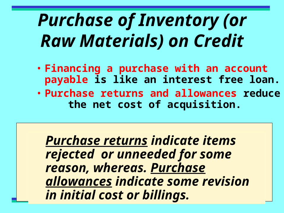
Purchase of Inventory (or Raw Materials) on Credit

• Financing a purchase with an account payable is like an interest free loan.

• Purchase returns and allowances reduce the net cost of acquisition.

Purchase returns indicate items rejected or unneeded for some reason, whereas. Purchase allowances indicate some revision in initial cost or billings.

Purchase Discounts(e.g., 2/10, n/30)

Purchase discounts ...

• Encourage early payment.

• Reduce the net cost of inventory.

• Create significant savings (a missed purchase discount of just 2% to pay 20 days earlier than a due date, equates to suffering a 36% interest rate)!

Computation of Net Purchases(in the Income Statement)

• In the Costs of Goods Sold disclosures:

– Purchases

– Less: Purchase discounts taken

– Less: Purchase returns and allowances

The exact location of subtotals in the format is a matter of preference.

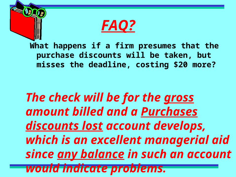
FAQ?

What happens if a firm presumes that the purchase discounts will be taken, but misses the deadline, costing $20 more?

The check will be for the gross amount billed and a Purchases discounts lost account develops, which is an excellent managerial aid since any balance in such an account would indicate problems.

Computation of Net Purchases(in the Income Statement)

• In the Costs of Goods Sold disclosures:

– Purchases

– Less: Purchase discounts taken

– Less: Purchase returns and allowances

The exact location of subtotals in the format is a matter of preference.

Purchases ($750,000 x 97%) $727,500

Purchase returns and allowances ($25,000 x 97%) (24,250)

Net purchases $703,250

ALTERNATIVELY:

Purchases $750,000

Purchase returns and allowances (25,000)

725,000

Purchase discounts ($725,000 x 3%) (21,750)

Net purchases $703,250

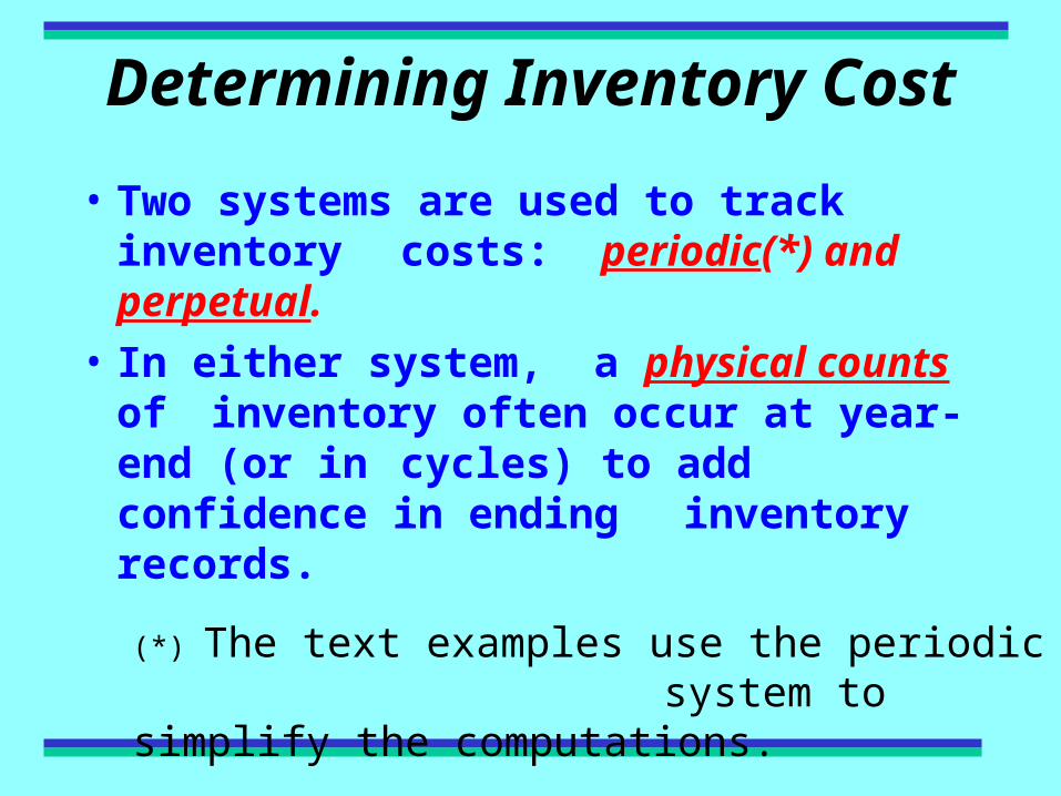
Determining Inventory Cost

• Two systems are used to track inventory costs: periodic(*) and perpetual.

• In either system, a physical counts of inventory often occur at year-end (or

in cycles) to add confidence in ending inventory records.

(*) The text examples use the periodic system to simplify the computations.

FAQ?

Two companies are contrasted in the following display of the Cost of goods sold section of an Income Statement.

Which company is in manufacturing (and what do the abbreviations mean)?

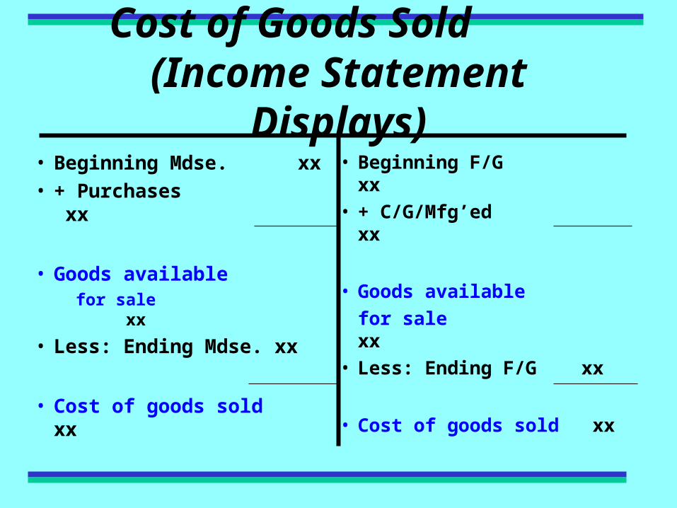
Cost of Goods Sold (Income Statement Displays)

• Beginning Mdse. xx• + Purchases xx

• Goods availablefor sale xx

• Less: Ending Mdse. xx

• Cost of goods sold xx

• Beginning F/G xx• + C/G/Mfg’ed xx

• Goods available

for sale xx• Less: Ending F/G xx

• Cost of goods sold xx

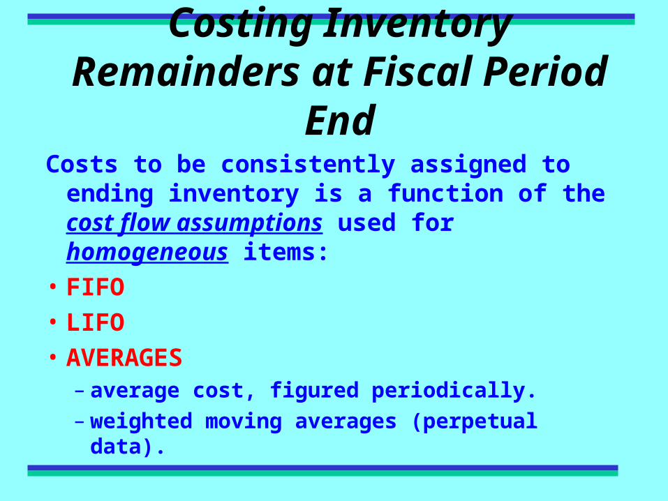
Costing Inventory Remainders at Fiscal Period End

Costs to be consistently assigned to ending inventory is a function of the cost flow assumptions used for homogeneous items:

• FIFO

• LIFO

• AVERAGES – average cost, figured periodically.– weighted moving averages (perpetual data).

FAQ?

What about non-homogeneous items?

The presumption is that unique items would be such that the specific identification method would apply (e.g., artworks, cars, antiques, race horses). Individual tagging of items, if practical!

Basic Cost Flow Assumptions• FIFO (first-in, first-out): Units sold are

assumed to be first units purchased (ending inventory = costs of the last purchases).

• LIFO (last-in, first-out): Units sold are assumed to be last units purchased (ending inventory = cost of the first units purchased).

• Average (periodic): Unit cost = [cost of beginning inventory + cost of purchases] divided by the total units involved; thus, ending inventory = unit cost x units on hand!

Inflationary Trends Mean ...

• FIFO: Ending inventory is costed using nearest-to-year-end replacement costs.– Old [lower] costs were matched to sales, which

produces “a higher reported gross profit.”

• LIFO: Ending inventory is costed using nearest-to-year-start (oldest) costs.– New [higher] costs were matched to sales,

which produces “a low reported gross profit.”

[The opposite types of results are reported during deflationary times.]

FAQs?

Is LIFO common in international business? Is LIFO, which is acceptable per GAAP, also OK for income tax purposes?

No. The U.S. is the only major country to allow LIFO. As to taxes, if LIFO is used for financial reporting purposes, the IRS requires that it be used for tax purposes!

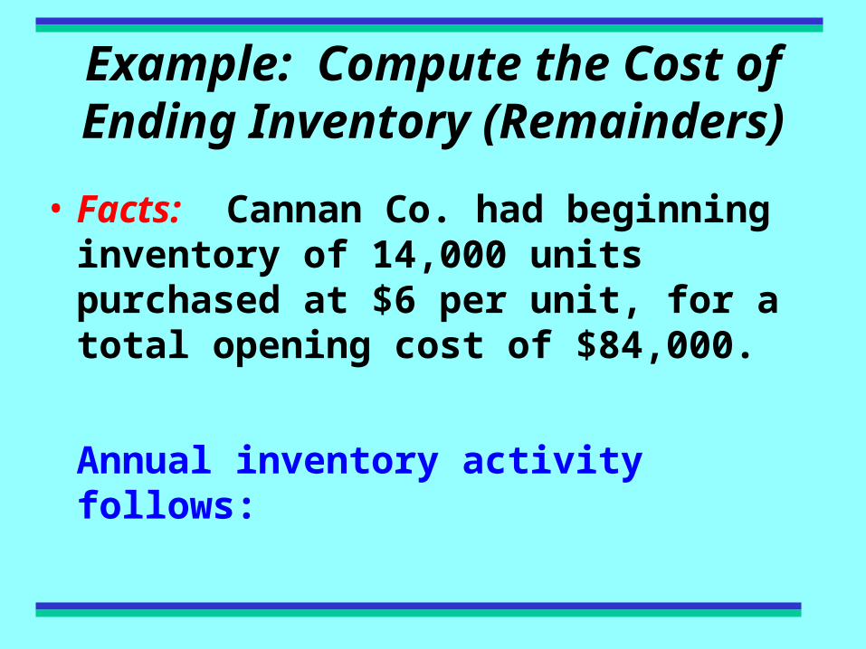
Example: Compute the Cost of Ending Inventory (Remainders)

• Facts: Cannan Co. had beginning inventory of 14,000 units purchased at $6 per unit, for a total opening cost of $84,000.

Annual inventory activity follows:

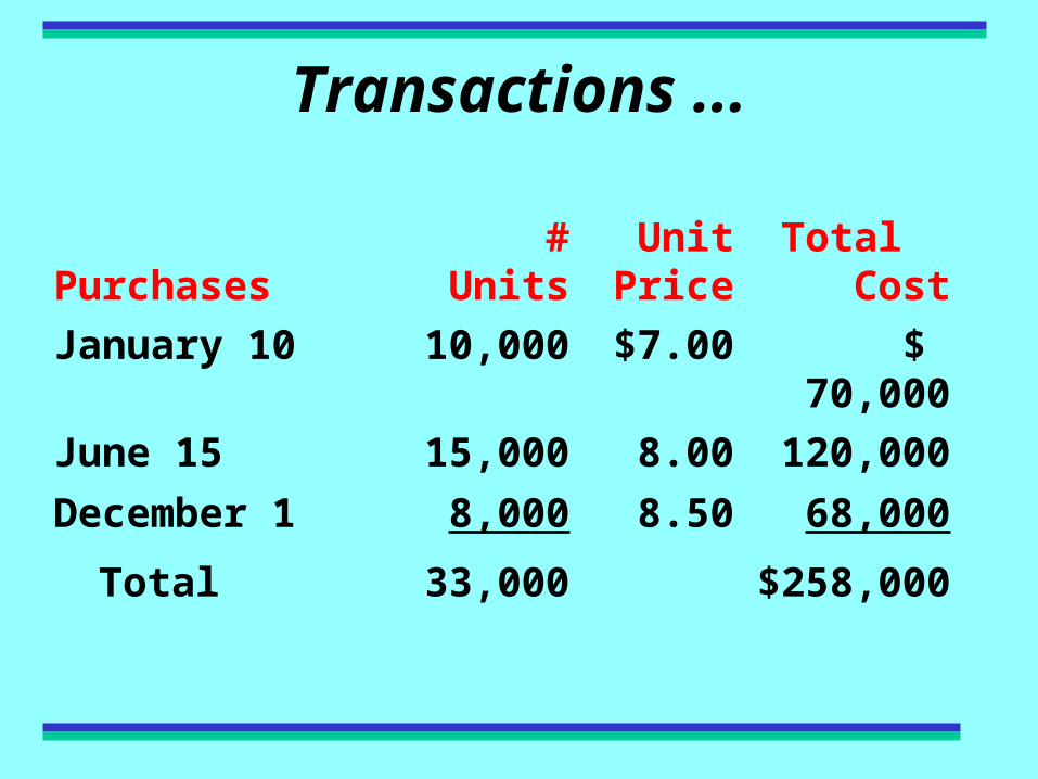
Transactions ...

Purchases # UnitsUnit

PriceTotal

Cost

January 10 10,000 $7.00 $ 70,000

June 15 15,000 8.00 120,000

December 1 8,000 8.50 68,000

Total 33,000 $258,000

Sales # UnitsUnit

PriceTotal

Cost

February 15 7,000 $15 $105,000

May 1 5,000 16 80,000

October 1 11,000 17 187,000

December 15 15,000 18 270,000

Total 38,000 $642,000

Calculate ending inventory, cost of goods sold and gross profit under three [periodic] methods: LIFO, FIFO, Average.

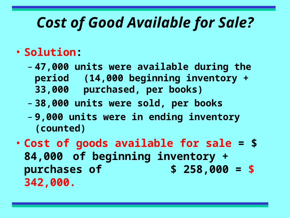
Cost of Good Available for Sale?

• Solution: – 47,000 units were available during the period

(14,000 beginning inventory + 33,000 purchased, per books)

– 38,000 units were sold, per books– 9,000 units were in ending inventory (counted)

• Cost of goods available for sale = $ 84,000 of beginning inventory + purchases of

$ 258,000 = $ 342,000.

LIFO Assumption

• Ending Inventory = $54,000The cost of the first 9,000 units purchased: 9,000

beginning inventory x $6

• Therefore, Cost of Goods Sold = $288,000 Details: (8,000 x $8.50) + ($15,000 x $8) +

(10,000 x $7) + (5,000 x $6)

• Check: $54,000 + $288,000 = $342,000, the cost of goods available for sale

FIFO Assumption• Ending Inventory = $76,000

The cost of the first 9,000 units purchased: (8,000 x $8.50) + (1,000 x $8)

• Therefore, Cost of Goods Sold = $266,000Details: (14,000 x $6) + (10,000 x $7) +

(14,000 x $8)

• Check: $76,000 + $266,000 = $342,000, the cost of goods available for sale

Periodic Averaging• Average Cost = $7.2766

Math: $342,000 cost of goods available for sale 47,000 units available for sale

• Ending Inventory = $65,489Math: 9,000 units x $7.2766

• Therefore, Cost of Goods Sold = $276,511Math: 38,000 units x $7.2766

• Check: $65,489 + $276,511 = $342,000, the cost of goods available for sale

Weighted Moving Average Cost

An excellent alternative provides a perpetual reading on the cost of inventory on hand. After every purchase, a new average is calculated (based on the prior balance plus the purchased items). Any items sold are issued at the then-current average cost.

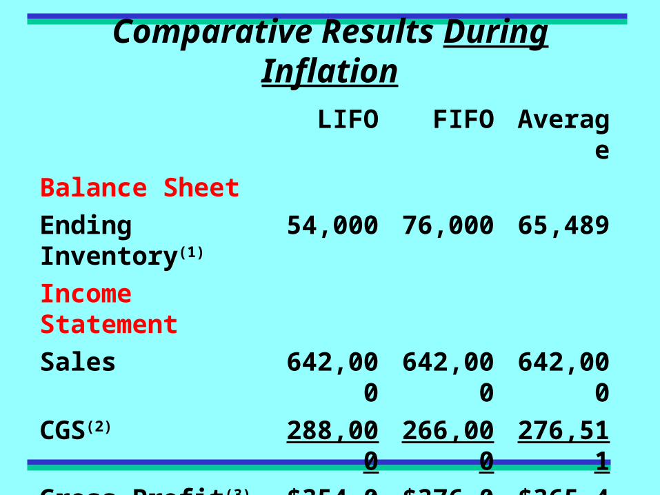
Comparative Results During Inflation

LIFO FIFO Average

Balance Sheet

Ending Inventory(1) 54,000 76,000 65,489

Income Statement

Sales 642,000 642,000 642,000

CGS(2) 288,000 266,000 276,511

Gross Profit(3) $354,000 $376,000 $365,489

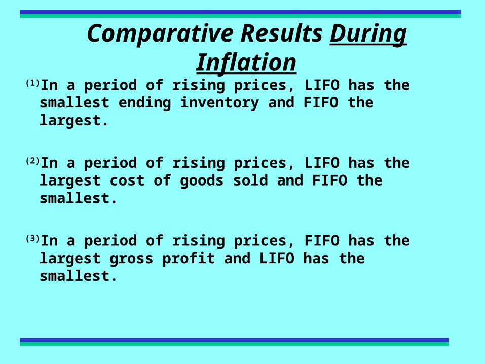
Comparative Results During Inflation(1)In a period of rising prices, LIFO has the smallest

ending inventory and FIFO the largest.

(2)In a period of rising prices, LIFO has the largest cost of goods sold and FIFO the smallest.

(3)In a period of rising prices, FIFO has the largest gross profit and LIFO has the smallest.

Balance Sheet Presentation Using an LCM Adjustment!

• Inventory is often reported at the lower of cost or market (LCM) to be conservative:– Cost is initially determined by an

inventory cost method (specific identification, LIFO, FIFO, Average)

– Market: Current replacement cost, subject to the following constraints:

• Market cannot be more than a ceiling amount, net realizable value (NRV).

NRV: Sales price minus cost to complete and dispose of the item.

• Market cannot be lower than a floor amount: NRV minus a NPM.

Using NPM, a normal profit margin, is theoretically sound; it means that no profit is recognized until a sale is made!

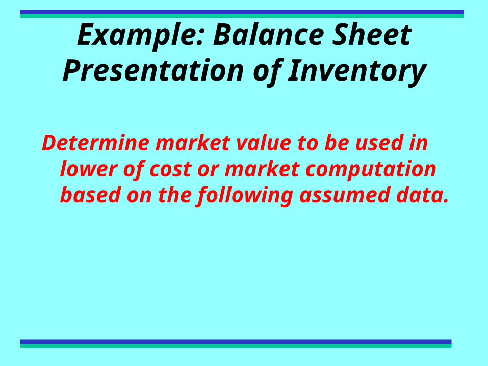
Example: Balance Sheet Presentation of Inventory

Determine market value to be used in lower of cost or market computation based on the following assumed data.

Illustration: Deriving “Market” for LCMCase Ceiling(1) R.C.(2) Floor(3) Market(4)

A $80 $60 $30 $60

B 80 45 30 45

C 80 90 30 80

D 80 90 30 80

E 80 25 30 30

Note: Designated market is the middle of the three market values in all cases; it neither exceeds the ceiling nor is lower than the floor

(1) Ceiling = NRV

(2) R.C. = Current replacement cost

(3) Floor = NRV – NPM

(4) Designated market, used for computing LCM by comparing market to cost.

Determining Lower of Cost or Market

Case Designated Market Cost (1)

Balance Sheet Valuation

A $60 $ 50 $50

B 45 50 45

C 80 50 50

D 80 100 80

E 30 100 30

(1) Determined by “regular” inventory costing method (e.g., LIFO).

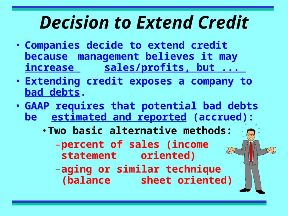
Decision to Extend Credit• Companies decide to extend credit because

management believes it may increase sales/profits, but ...

• Extending credit exposes a company to bad debts.• GAAP requires that potential bad debts be

estimated and reported (accrued):• Two basic alternative methods:

– percent of sales (income statement oriented)

– aging or similar technique (balance sheet oriented)

Observation!

The “direct write-off” method: No bad debt is recognized until a specific customer’s account is identified for a write-off.

Unacceptable under GAAP!

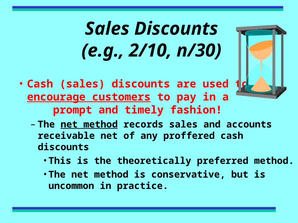
Sales Discounts(e.g., 2/10, n/30)

• Cash (sales) discounts are used to encourage customers to pay in a prompt and timely fashion!– The net method records sales and accounts

receivable net of any proffered cash discounts• This is the theoretically preferred method.• The net method is conservative, but is

uncommon in practice.

Example: Sales on Account

• A company sells inventory with a cost of $150,000 for $240,000, with terms 2/10, net 30:– Customer is offered a 2% cash discount if paid

within 10 days.– Sales and account receivable recorded at

$235,200: $240,000 x 98% = $235,200

– If sales discount is not taken, the $4,800 would be considered as interest income.

Examples: Bad Debts Expense

• “Percent of credit sales” method– The Spivey Co. believes that 4% of credit sales

will never be collected; Spivey recorded $20,000,000 in

credit sales during the year.• Spivey records $800,000 in bad debts

expense! • The Bad debts expense = f(credit sales)

• “Aging” (or similar) method– The Landers Co. uses the aging method.

At year end, an aged analysis indicates that $150,000 is a likely amount of receivables to remain uncollected.

– The current balance in the allowance for uncollectible accounts is $25,000 (credit).• Landers increases the allowance by $125,000,

from $25,000 to $150,000.• The Allowance account = f(A/R balance)

Sales Returns

• Any sales returns by customers reduces accounts receivable and is a part of

the calculation of net sales.

• An Allowance for estimated sales returns should appear on the Balance Sheet as a contra asset. (Rare in practice!)

Using Accounts Receivableto Increase Liquidity

(Borrowing Against Receivables or Selling Receivables)

Borrowing using accounts receivable as collateral

• Specific assignment (specific receivables are designated as collateral)

• General assignment (all receivables are designated as collateral)

• With recourse: If the receivables are not collected, the factor can look to the

seller company for payment.• Without recourse: If the receivables are not

collected, the factor cannot look to the seller company for payment.

Selling accounts receivable to a Factor (Factoring):

Short-Term Trade Notes Receivable

If accepted in return for sale of inventory, the notes receivable are designated as Notes Receivable - Trade in the Balance Sheet.

• Record at face value.

• Accrue interest revenue separately.

• The SCF reflects cash flows from trade notes receivable under Operating Activities.

Statement of Cash Flows:

Indirect Method• The cash flows from selling inventory to

customers are Operating Activities, but• The SCF using an indirect method is used

by many publicly traded companies. • The indirect method starts with net income

then adjusts for certain items to reconcile to cash flow from operating activities

• Noncash expenses and revenues.

• Non-operation gain and losses.

• Operational balance sheet accounts for which cash basis accounting and accrual basis accounting give

differing results.

Categories of reconciling items in indirect method for SCF:

Indirect Method Adjustments

• Cash flow from operating activities– Net Income– Add (Deduct)

• Non-cash expenses (e.g., depreciation, depletion, amortization) (1)

• (Non-cash revenues) (e.g., investment income for securities accounted for under the equity method) (1)

• Losses (gains) on sales(2)

• Decreases (increases) in operational current assets and deferred income tax assets (3)

• Increases (decreases) in operational current liabilities and deferred income tax liabilities (3)

• Net cash flows from operating activities

The indirect approach to a SCF is thought by many to be somewhat difficult to interpret.

Documentation(1) Non-cash expenses and revenues affect net

income, but not cash.(2) Gains and losses are non-operational in

nature for most companies.(3) Reconciling items adjust from the accrual

basis effects, reflected in net income, to the cash basis effects. (Deferred income tax assets and liabilities are discussed in Chapter 11.)

End of Chapter 9