Embed Size (px)
Citation preview

1
Man on the Bench: The Power of the Stick in the Sales Force
Abstract Sales leaders often use both carrots (e.g., commission) and sticks (e.g., punishment) to manage
the sales force. Yet astonishingly little research has examined the effect of sticks on
performance. The current research addresses this gap by investigating an intervention called the
“man-on-the-bench” program in a quasi-experimental field setting. In treatment districts, the
company told salespeople that a trainee sitting on the bench would replace them at the end of the
program year if they failed to hit quota and fell into the last place. Difference-in-differences
analyses of matched treatment and control groups show that the program had an immediate and
sustained impact on both low-performing salespeople and salespeople who sought advice from a
greater number of peers. A laboratory study follows the field study to compare the man-on-the-
bench program with other kinds of sticks commonly used in practice. The results suggest that the
effect of a bench is greater than that of merely displaying relative performance or threatening job
loss for missing quota. The latter result suggests that the vividness of a threat exerts an increased
effect on performance.
Keywords: sales force, carrots, sticks, advice networks, field experiment, matching methods

2
A broad range of analytic, empirical, and experimental research has examined sales force
compensation plans (e.g., Basu et al. 1985; Coughlan and Narasimhan 1992; Lim, Ahearne, and
Ham 2009; Steenburgh 2008). Primarily focused on the design of optimal incentive contracts,
that research has generated various prescriptions for the use of compensation instruments known
informally as “carrots” (e.g., variable pay, bonuses, contests). For example, a general
recommendation is that high-powered incentive contracts should be used when salesperson effort
is costly to monitor (see Banerjee et al. 2012). However, missing from this research are
prescriptions for the use of accountability instruments, known informally as “sticks” (e.g.,
threatened punishment, social pressure).
This omission exists despite estimates suggesting that somewhere between 25% and 50%
of Fortune 500 companies aggressively use threatened punishment to manage their bottom
performers (Grote 2005). Threatened punishment is often levied with rules that companies devise
for salesperson dismissal or with employee fines and penalties. Jack Welch implemented the
most widely known example of this practice when he was chief executive officer of General
Electric. During his tenure, the bottom 10% of performers were fired on an annual basis (Welch
and Byrne 2003). Other companies devise rules to threaten punishment based on performance
floors. They mandate the attainment of certain commission levels or enforce minimum year-
over-year growth objectives to determine firing decisions (Smith 2012).
Reasons for threatening punishment with top-down accountability systems or enacting
social pressure programs stem from sales managers’ hesitation to enforce negative incentives
with low-performing salespeople. In addition, when deciding whether or not to replace chronic
low performers, sales managers generally place too much weight on sales force turnover costs,
including costs associated with recruitment and selection, training, and territory vacancy

3
(Darmon 1990). These costs are no doubt an unavoidable consequence of dismissing salespeople
in many instances. However, successful companies understand that removing or, at the very
least, taking corrective action on poor performers is necessary to remain competitive.
With punishments or sticks playing such an important role in companies’ talent
management practices, it is puzzling that an established empirical literature has yet to develop
(See Table 1). As Scullen, Bergey, and Aiman-Smith (2005, p. 26) state, there is “almost no
supporting research base currently available”. What is clear is that the primary reason for such
scarcity is that data are difficult to obtain. Even the sales force incentive literature has suffered
from a shortage of empirical data (see Misra and Nair 2011). As sticks are a more sensitive issue
to companies than carrots, researchers face a particularly uphill battle collecting data in this
realm. As a result, no research has investigated the impact of sticks on salesperson performance
using company data. Aside from a stream of research based on experiments in the economics
literature (e.g., Dickinson 2001; Fehr and Schmidt 2007), extant literature is void of work in this
area.
----- Insert Table 1 about here -----
To alleviate this shortcoming, we examine a novel type of stick, which we term the
“man-on-the-bench” (MOB) program. We use this nomenclature because the program closely
matches the impact of bench players on starters in sports. It introduces inactive salespeople (i.e.,
bench players) to sales districts and imparts formal rules to determine whether they will replace
current salespeople (i.e., starters) after a pre-specified period. We conduct two studies to test the
effect of the MOB program. In Study 1, we investigate the impact of the MOB program using a
field-based quasi-experiment, in which trainees (i.e., bench players) were hired into a subset of
the company’s sales districts (treatment districts) and incumbent salespeople were told that a

4
trainee would replace them at the outset of the program if they missed their annual quota and fell
into last place in their district. Importantly, this bench threat was not applied in control districts
and was discontinued after its first year. We examine (1) the effect of the MOB program on
performance during the year it was implemented, (2) the effect of the MOB program on
performance after it was discontinued, and (3) which salespeople were most influenced by the
MOB program. In Study 2, a lab experiment with 180 students, we extend Study 1 by comparing
the MOB program with other types of sticks: displaying relative performance and firing for poor
performance.
In Study 1, we find that (1) the MOB program improved performance during the year it
was implemented by an estimated 3.66%, (2) survivors’ performance in the post-program year
fell by 3.29% to revert to near preprogram year levels, and (3) these effects varied depending on
salesperson past performance and social connections. Specifically, the treatment and
posttreatment effects of the MOB program were concentrated at the lower end of the
performance distribution. In addition, salespeople were more likely to improve their performance
during the MOB program if they had a higher number of advice networks, but the loss of a
central salesperson in these districts led to lower performance in the year following the MOB
program. Study 2 further shows that the MOB program is superior to merely displaying relative
performance or firing for poor performance but without a replacement in sight. This latter result
suggests that the vividness of threat of the replacement further enhances performance.
This research makes four important contributions. First, by shifting the focus from carrots
to sticks, we introduce an important type of motivational tool in sales force management. As
firms find it difficult to manage their sales force, especially the bottom performers, our empirical
evidence indicates that sticks can be a powerful tool in managing the sales force. Second, we

5
contribute to the literature on sales force turnover by suggesting that having a replacement
available lowers turnover costs. The turnover costs of a sales force can lead to an annual sales
loss of 13.2%–17.6% (Shi et al. 2017). As a result, managers are generally reluctant to dismiss
the bottom-performing salespeople. The MOB program addresses this issue by decoupling the
factors associated with turnover, such as recruitment and selection, training, and territory
vacancy, from sales managers’ dismissal decision. As the reserve salesperson gains required
knowledge and skills during the MOB program, he or she should be able to connect seamlessly
with customers, thereby avoiding loss of sales. Third, we contribute to the nascent literature on
sales force social networks. Prior work has demonstrated that the salespeople with better
connections with other salespeople have superior performance (Bolander et al. 2015). We
complement this research by examining the role of social networks in the context of punishment.
Our results indicate that the salespeople with better connections can cope better with sticks.
More important, firing a “central” salesperson negatively affects the performance of the
remaining salespeople. Fourth, we contribute to the literature on sticks in general. The limited
research in this area relies mostly on lab experiments. To the best of our knowledge, our study is
the first to examine the role of sticks in a field experiment spanning multiple years. Furthermore,
whereas prior research suggests that pure incentives are preferable to a combination of incentives
and punishments (Fehr and Schmidt 2007), we demonstrate that punishments can enhance
performance. We attribute the discrepancy in results to the level of punishment: previous
research used fines as a proxy for punishment, and we use job threat as punishment.
We elaborate on these findings and explicate their theoretical and managerial
implications in the “General Discussion” section. Prior to then, the paper flows from establishing
hypotheses to outlining the empirical methods we use and reporting the results of the study.
6
HYPOTHESES DEVELOPMENT
The Effect of the MOB Program
Expectancy theory (Vroom 1964), first applied to the sales literature by Walker,
Churchill, and Ford (1977), holds that motivation depends on three factors: expectancy, or the
belief that effort will result in performance; valence, or the desirability of rewards associated
with performance; and instrumentality, or the belief that performance will be met with rewards.
Whereas Kumar, Sunder, and Leone (2014) use expectancy theory to explain why monetary
incentives positively influence salespeople’s future value, we apply it to inform our predictions
about the positive influence of threatening punishment. Overall, expectancy theory suggests that
threatening punishment should serve as extrinsic motivation for salespeople when they (1)
believe that applying extra effort could help them avoid being punished, (2) desire to avoid what
is being threatened, and (3) believe threats will be enforced if performance standards are not met.
In the context of the MOB program, salespeople are at risk of losing not only their bonus
but also their job if they miss quota. Expectancy theory suggests that these salespeople should
perform better than they would without the threat of punishment so long as they (1) believe they
can hit quota, (2) desire to work for the company, and (3) believe the company will fire them for
missing quota and falling into the last place in their district. With these assumptions, we expect
the MOB program to positively influence salesperson performance. Research also suggests that
employees perform better if doing so reduces job insecurity (Cron, Dubinsky, and Michaels
1988), partially because extra effort serves as a coping strategy (Gilboa et al. 2008). Because
lower-performing salespeople need to improve more to hit quota, we expect the MOB program
to have an even greater influence on these performers.
We are also interested in the role of advice networks on the effect of the MOB program.
Defined as the extent to which salespeople go to others for advice, out-degree centrality may

7
moderate the effect of the MOB program because “people generally seek social support in times
of threat” (Smith, Menon, and Thompson 2012, p. 69) and open communication lines should
make reaching out to others for help or advice relatively easier. To the extent that research has
found advice sharing in sales to facilitate the transfer of actionable knowledge (Bolander et al.
2015), salespeople with more resources to tap into should be able to improve their performance
more than salespeople with fewer resources at their disposal. Accordingly, from these arguments,
we hypothesize the following:
H1: (a) Introducing the MOB program will increase salespeople’s year-over-year
performance. This effect will be greater for (b) lower performers and (c) salespeople with
greater out-degree centrality.
The Effect of Discontinuing the MOB Program
Removing the threat of punishment ultimately reduces salespeople’s incentives to hit
quota, because it relieves their assumption that poor performance will be met with job loss. In
line with expectancy theory, we, therefore, expect survivors of the MOB program to decrease
their performance. Without trainees in MOB districts and without formal rules for dismissal, the
incentive to meet quota or to avoid finishing in last place in a district is removed. This situation
is comparable to postlayoff conditions, in which layoff survivors have been found to reduce their
performance to baseline levels (Probst 2002). Part of the reason for this reduction is that
survivors become complacent (Brockner et al. 1992). Another explanation is that survivors tend
to rationalize their status as survivors psychologically (Brockner et al. 1986). As such, they
believe that their past performance justifies their status as a survivor, and in turn, they do not feel
obligated to continue performing at higher-than-baseline levels. As we expect performance

8
relative to baseline to be higher for lower performers, we expect low-performing survivors to
decrease their performance more than high-performing survivors.
We also expect survivors in districts that lose a salesperson to decrease their performance
more if their district loses a salesperson that is central to the advice network. Our rationale for
this expectation is that replacing a central salesperson in a district disrupts the flow of
information and thereby hinders survivors’ performance. By contrast, we do not expect this
pattern of results for survivors in districts. Accordingly, we hypothesize the following.
H2: (a) Discontinuing the MOB program will decrease survivors’ year-over-year
performance. This effect will be larger for (b) lower performers and (c) survivors in
districts that lose a salesperson with higher in-degree centrality.
To test our hypotheses, we conducted two studies. Study 1 is a field-based quasi-
experiment. Study 2 is a laboratory experiment, in which we compare the effectiveness of the
MOB program with other “sticks” commonly used in practice.
STUDY 1: FIELD-BASED QUASI-EXPERIMENT
Institutional Details and Study Outline
The empirical context of this study is a Fortune 500 company that sells cleaning and
sanitation supplies to the restaurant and hospitality industry. The company’s salespeople sell its
products within territories that are organized in districts, overseen by district managers, and
dispersed across the United States. Salespeople at the company earn approximately $40,000 in
salary per year, on average, plus commissions and a $2,000 bonus for meeting an annual quota.
Before the studied intervention, the company had a supportive culture and had not
dismissed a salesperson for poor performance in more than two years. However, its executives

9
were concerned that this culture had led a proportion of its sales force to shirk, and the
company’s vice president of sales suggested hiring trainees as potential replacements of low
performers. We worked with the company to design a quasi-experiment and to test the effect of
this intervention empirically.
The research design of the study is as follows: In 58 treatment districts, managers
announced the MOB program at the beginning of the program year. Incumbent salespeople were
told that a trainee (i.e., bench player) would be hired into their district later in the year and that
this person would replace the lowest-performing salesperson in their district if that individual
failed to meet annual quota. Alternatively, if every salesperson in a district achieved quota, all
would stay in their roles, and the trainee would be assigned to another open position in the
company. Trainees learned the job by working with district managers. They did not help or
shadow salespeople during the training period. Their time “on the bench” was spent earning
certificates and engaging in technical training. As is typical in technical sales roles, salespeople
at this company are required to install heavy equipment in addition to their regular selling
activities, which results in an extensive ramp-up period for new hires. In the company’s other 82
districts (i.e., the control group), operations did not change, and trainees were not hired.
After the program year, 46 salespeople from MOB districts were replaced by trainees for
missing quota in the program year and being the lowest performers in their districts. Although
the senior vice president of sales who introduced the MOB program deemed the program
successful, other members of the senior management team were concerned that the program
would adversely affect the culture of the company. Therefore, the executive team decided not to
roll it out across the company and not to continue it in MOB districts. For research purposes, this
situation opened up an opportunity for us to examine the posttreatment effects we included in H2.

10
Data and Variable Definitions
The data we analyze come from three sources. The first is the company’s performance-
tracking database, from which we use salespeople’s performance in the preprogram, program,
and postprogram years to measure the effectiveness of the MOB program. Second, in the latter
half of the preprogram year, we collected advice-network data. Salespeople were asked to name
colleagues in their districts who they go to for advice about work-related matters. Using
established procedures (Scott 2012), we counted how many colleagues a given salesperson
reported and assigned this number to a variable called “out-degree centrality”. We also counted
how many colleagues reported going to a given salesperson for advice and assigned this number
to a variable called “in-degree centrality.” Third, we merged these performance and advice-
network data sets with variables from the company’s human resource records (i.e., tenure and
district size) to arrive at the final data set.
The performance data indicate salespeople’s sales in dollars relative to an expected
individual-based quota, which was set for every salesperson across the company by an external
firm that specializes in sales compensation. This percent-to-quota measure is a useful metric
because quotas account for differences in factors such as territory potential, number of existing
customers, and size of existing customers. For these reasons, percent-to-quota is widely
considered a valid performance metric for sales force research (Churchill et al. 1985; Zoltners,
Sinha, and Lorimer 2006).
Although the company’s performance-tracking database has performance data for every
salesperson in the company, nonresponse led to missing values in the advice-network data. Of
the 699 salespeople in the company, 526 participated in the advice-network survey, representing
a 75% response rate. To assess whether nonresponse bias is an issue, we compared salespeople

11
who participated in the survey with those who did not participate. The results of these tests show
that the two groups do not differ in terms of salesperson tenure, district size (number of
salespeople per district), or performance. We also tested whether nonresponse differed across
districts in the MOB program and those in the control condition, similarly finding nonsignificant
results. In turn, we felt confident analyzing the complete data set after replacing missing values
of the out-degree and in-degree centrality variables with their grand means. Nevertheless, we
reran the analyses with only the salespeople who responded to the advice-network survey in the
data set and found materially similar results (i.e., all hypotheses continued to receive support).
In summary, we collected the following variables: tenure, measured as the number of
years a salesperson had been with the company; district size, or the number of salespeople
assigned to a district; salesperson performance, measured in percent form as dollar sales relative
to quota; and out-degree/in-degree centrality, calculated as the number of colleagues who a
given salesperson reported going to for advice or the number of colleagues who reported going
to a given salesperson for advice. Table 2 reports the descriptive statistics of these variables for
MOB districts, control districts, and all districts.
----- Insert Table 2 about here -----
Quasi-experimental Design and Matching Procedure
Although we maintained close contact with the company throughout the study, we were
not able to convince the executive team to assign trainees to districts at random. Therefore, the
quasi-experimental design we adopt compares the performance of salespeople from MOB
districts with the performance of comparable salespeople from control districts, who were
selected by a matching procedure. This approach has advantages over research designs without
control groups, insofar as having a control condition accounts for extraneous events that would

12
artificially produce a treatment effect in lieu of the MOB program. For example, if a competitor
recalled its product during the program year and companywide sales increased as a result, the
influence of the MOB program would be inestimable without control districts. This hypothetical
scenario and similar confounds do not hurt the internal validity of our study because both MOB
and control districts would be affected and a treatment effect (i.e., differential rise in
performance) would not emerge in their presence without a true effect of the MOB program.
Yet causal inferences are only possible to the extent that a comparable control group is
available. While random assignment was not feasible, the executive team did agree not to target
districts with low-performing salespeople when deciding which districts to include in the MOB
program. In the end, the company’s executive team assigned 58 districts to the MOB program
and 82 districts to the control condition. As Table 2 shows, the average preprogram year
performance was about the same in the treatment and control conditions: 96.45% in MOB
districts versus 96.37% in control districts. This similarity corroborates the company’s claim that
low-performing districts were not targeted.
To further ensure that the treatment and control groups were comparable, we used
matching methods to improve the balance between the groups on several variables. Matching
achieves balance by transforming quasi-experimental data to resemble that which a randomized
experiment might generate (Ho et al. 2007). The variables we match on are salesperson tenure,
district size, preprogram performance (two years before, one year before, and variability), and
out-degree centrality. The 413 salespeople who worked in control districts were available to be
selected as matches of the 286 salespeople in MOB districts. For the variables, Table 3, Panel A,
reports standardized mean differences, a statistic that represents differences in means between
MOB and control districts on a given variable divided by the standard deviation of MOB districts

13
with respect to that same variable. A rule of thumb is that better balance between groups is
required if the standardized mean difference is greater than .25 (Avery et al. 2012). As the
unmatched column of Panel A of Table 3 shows, the MOB and control districts were reasonably
balanced across most variables. In particular, the standardized mean differences for preprogram
performance fell well below the .25 cutoff.
----- Insert Table 3 about here -----
However, the treatment and control groups were imbalanced on the out-degree centrality
measure. A standardized mean difference of .30 indicates that salespeople in MOB districts
reported seeking advice from a greater number of others than salespeople in control districts.
Therefore, in line with the work of Ho et al. (2007), we implemented and evaluated five
matching procedures (i.e., nearest neighbor, optimal, subclass, full, and genetic) to bring the two
groups into balance on this variable, while still maintaining balance on the other three variables.
As Diamond and Sekhon's (2013) genetic matching procedure arrived at the most well-balanced
match, we used it to create the matched data set. Importantly, this genetic matching procedure
(please see Web Appendix for an outline of this procedure) brought the standardized mean
difference on the out-degree centrality variable down to zero (see Table 3, Panel A). All other
variables remained in balance after the match as well. The largest absolute standardized mean
difference across the variables is .04, which falls well below the .25 cutoff. The resulting
matched data set retained all 286 salespeople from MOB districts and included 188 salespeople
from control districts.
Next, to assess the posttreatment effect for the year after the MOB program was
discontinued, we matched survivors of the MOB program with comparable salespeople from
control districts (whom we also refer to as survivors, for convenience, even though they were not
14
at risk of losing their jobs). Following the same steps as before, we found that the genetic
matching procedure again generated the most-balanced data set. The largest standardized mean
difference after matching was again .04 (see Table 3, Panel B), and the resulting matched data
set retained all 240 survivors of the MOB program and included 159 comparable survivors from
control districts.
In summary, to prepare for parametric analyses, we matched salespeople who were
assigned to the MOB program, as well as survivors in the MOB program, with comparable
others from control districts. In what follows, we detail the econometric models we use to
evaluate the treatment and posttreatment effects.
Model Specification
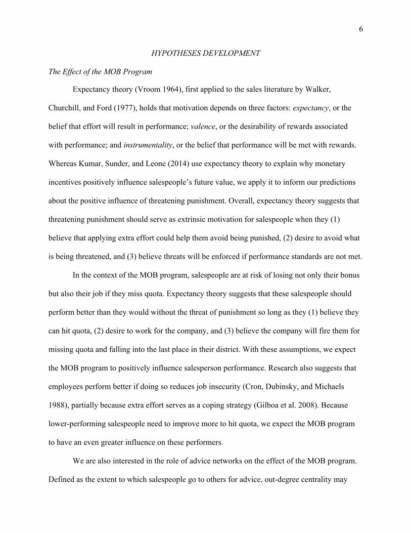
We begin this section with the model we specify to test H1a, which aims to assess whether
the MOB program increased salesperson performance during the program year:
yikt = α + β1Ti + β2Oi + β3Pt + β4MOBk + β5TEkt, (1)
where yikt is salesperson i in district k’s percent-to-quota during year t. This model is focused on
the preprogram and program years, so t takes the value of 1 and 2, respectively. Tenure, Ti, is the
number of years salesperson i had worked for the company at the beginning of the preprogram
year. Out-degree centrality, Oi, is the number of people whom salesperson i reported going to for
advice at the time of the survey in the preprogram year. Program, Pt, is a step function that
represents the onset of the MOB program in the program year. It takes the value of 0 in the
preprogram year and 1 in the program year. MOB district, MOBk, is equal to 1 if salesperson i’s
district k was assigned to the MOB program and 0 otherwise. Finally, we estimate the treatment
effect, TEkt, with a dummy variable equal to 1 in the program year if salesperson i’s district k was
assigned to the MOB program and 0 otherwise.

15
Building on this foundation, the aim of H1b is to determine whether the MOB program
had a differing effect across the company’s performance distribution, which we evaluate by
estimating Model 1 in a quantile regression framework (Koenker 2005). Last, for H1c, with the
aim to assess whether the effect of the MOB program differed across salespeople with various
out-degree centralities, we add an additional term to Model 1 that interacts the treatment effect
with out-degree centrality (i.e., TEkt × Oi).
The aim of H2a is to understand how survivors of the MOB program performed the year
after the program was discontinued. As such, we estimate the following model, which builds on
Model 1 and includes additional terms that allow us to test the posttreatment effect with the data
set of matched survivors:
yikt = α + β1Ti + β2Oi + β3Pt + β4PPt + β5MOBk + β6TEkt + β7PTEkt. (2)
Model 2 covers the preprogram, program, and postprogram years, so t takes the value of 1, 2, and
3, respectively. Of the variables included in Model 1, the two variables with t subscripts affected
by the additional year of data in this model are program, Pt, and the treatment effect, TEkt. As
before, Pt takes the value of 0 in the preprogram year and 1 in the program year, but now it also
takes the value of 1 in the postprogram year. This modification changes TEkt to now equal 1 in
both the program year and the postprogram year if survivor i’s district k was assigned to the
MOB program and 0 otherwise. Regarding the new variables in Model 2, postprogram, PPt,
takes the value of 0 in both the preprogram year and the program year and 1 in the postprogram
year; we estimate the posttreatment effect, PTEkt, with a dummy variable equal to 1 in the
postprogram year if survivor i’s district k was assigned to the MOB program and 0 otherwise.
Building on the foundation of Model 2, we test H2b (i.e., whether the posttreatment effect
differs across the company’s performance distribution) with quantile regression. For H2c, we add

16
an interaction term to Model 2 that crosses the in-degree centrality of a district’s replaced
salesperson to capture with the posttreatment effect (i.e., PTEkt × Ik).
Results
In this section, we report a series of results that stem from the difference-in-differences analyses,
quantile regressions, and the two models specified previously. The structure of this presentation
flows according to the two hypotheses.
The treatment effect. We begin by testing the effectiveness of the MOB program during
the program year through difference-in-differences estimation. As Table 4, Panel A, shows, the
MOB program had a positive and significant effect on salesperson performance, in support of
H1a. That is, salespeople in MOB districts performed 4.07 percentage points higher, on average,
than would be expected if they were in a control district. We graphically depict this positive
treatment effect in Figure 1, Panel A, which plots the weighted averages of salesperson
performance (percent-to-quota) by condition and across time in months, which range from 1 to
24 months to cover the preprogram and program years.
----- Insert Table 4 and Figure 1 about here -----
Note that we are able to plot the data at a monthly level because the company breaks
annual quotas into monthly increments and tracks performance against these quotas throughout
the year. In addition, weights are an output of the genetic matching procedure because it matches
with replacement. Salespeople in MOB districts receive weights of 1, and salespeople in control
districts receive weights that reflect the frequency with which they were used as matches. We
used these weights to create Figure 1, Panel A, and they factor into all the other analyses we
conduct to make the treatment and control groups comparable (Ho et al. 2011).
As the differential slope after the vertical line in Figure 1, Panel A, highlights,
salespeople’s performance in MOB districts improved in the first month the program was put in

17
place (month 13) and continued at this higher level throughout the year. By comparison, the
control group’s performance did not change across the two years. This general pattern suggests
that the company’s salespeople were not harvesting achievable opportunities that existed in the
market, which could have resulted from their lack of effort. Furthermore, the improvement in
performance was immediate and remained at about the same level throughout the year. This
pattern suggests that salespeople were not playing timing games, such as forward selling, as
would be the case if salespeople were asking customers to buy earlier than they normally would
(Steenburgh 2008). If this practice had taken place, we would have observed a spike in business
at some point late in the program year and normal levels otherwise.
To test H1b, that lower performers in the MOB program will increase their performance
during the program year more than higher performers, we ran simultaneous quantile regressions
for nine deciles of the company’s performance distribution, ranging from the 10th to the 90th
percentile. We plot the treatment effects (and their 95% confidence intervals) for these nine
deciles in Figure 2, Panel A. As the panel shows, the points generally form a downward-sloping
line, with bottom performers increasing their performance by almost ten percentage points and
top performers being practically unaffected by the MOB program. A statistical test of the
difference between these two parameters resulted in a significant result (F = 17.51, p < .001). On
the whole, these analyses provide support for H1b and suggest that the MOB program had a
greater impact on lower-performing salespeople.
----- Insert Figure 2 about here -----
To determine the impact of the MOB program across performance levels, we also ran
separate difference-in-differences estimates for salespeople who were last-place performers,
second-to-last-place performers, and first-place performers in their districts in the preprogram

18
year. Here, we expected lower relative ranks to have larger treatment effects. Panel B of Table 4
shows that last-place performers in the MOB program performed 9.45 percentage points higher,
on average, than would be expected had they been in the control condition. In contrast, the
difference-in-differences estimate for second-to-last-place performers was 5.71 (Table 4, Panel
C), and that for first-place performers was 1.46 (Table 4, Panel D), a statistically nonsignificant
result. These results further suggest that the MOB program had its greatest effect at lower rungs
of the performance distribution within districts.
Furthering this line of analysis, Table 6 shows how mobility in rank differed across the
MOB program and control conditions. The rows are grouped by rank within districts in the
preprogram year (last place, second last place, and first place). For last-place performers and
second-to-last-place performers, we present the percentages that, in the program year, moved
down one rank, stayed the same, moved up one or two ranks, and moved up three or more ranks.
For first-place performers, we present the percentages that, in the program year, stayed in first
place, moved down one or two ranks, and moved down three or more ranks. Across all three
ranks, mobility occurred more frequently in MOB districts; last-place performers climbed the
ranks more often, second-to-last-place performers moved both up and down more frequently, and
a higher percentage of first-place performers fell in rank within their districts. These shifts
provide clear evidence that the MOB program increased rank mobility.
----- Insert Table 5 & 6 about here -----
Next, Table 5 explores how the treatment effect differed across levels of out-degree
centrality (H1c), and as the model shows, the interaction is both positive and significant (β = 1.60,
p < .001). This result indicates that the treatment effect was stronger for salespeople who
reported going to more colleagues for advice before the MOB program.

19
The posttreatment effect. Using the second matched data set (i.e., that which includes
three years of data for survivors of the MOB program and comparable salespeople from control
districts), we ran an extension of Model 2 to estimate the treatment effect and the posttreatment
effect for survivors of the MOB program. The results suggest that the MOB program had a
significant, positive effect in the program year (β = 5.27, p < .001) and that removing the MOB
program had a significant, negative effect in the postprogram year (β = –5.00, p < .001; see Table
7). Thus, in support of H2a, survivors of the MOB program decreased their performance in the
postprogram year, bringing them back to near preprogram year levels. We depict this general
pattern of results in Figure 1, Panel B, which plots the weighted averages of performance in the
MOB program and control conditions across time for the 36 months of the study.
----- Insert Table 7 about here -----
Estimating Model 2 in a quantile regression framework, we can determine whether
lower-performing survivors of the MOB program decreased their performance in the
postprogram year more than higher performing survivors (H2b). We depict the results of this
analysis in Figure 2, Panel B, which plots the posttreatment effects for nine deciles of the
company’s performance distribution, ranging from the 10th to the 90th percentile. As is evident
from the upward-sloping line, bottom-performing survivors of the MOB program decreased their
performance considerably following its removal, whereas top-performing survivors continued
performing at their normal levels. A statistical test of the difference between these two
parameters resulted in a significant result (F = 6.67, p < .01). In summary, these analyses provide
overarching support for H2b, which posits that lower-performing survivors of the MOB program
will decrease their performance during the postprogram year more than higher-performing

20
survivors. We also include Panel C of Figure 2 to provide graphical evidence of the treatment
effect for survivors of the MOB program across the performance distribution.
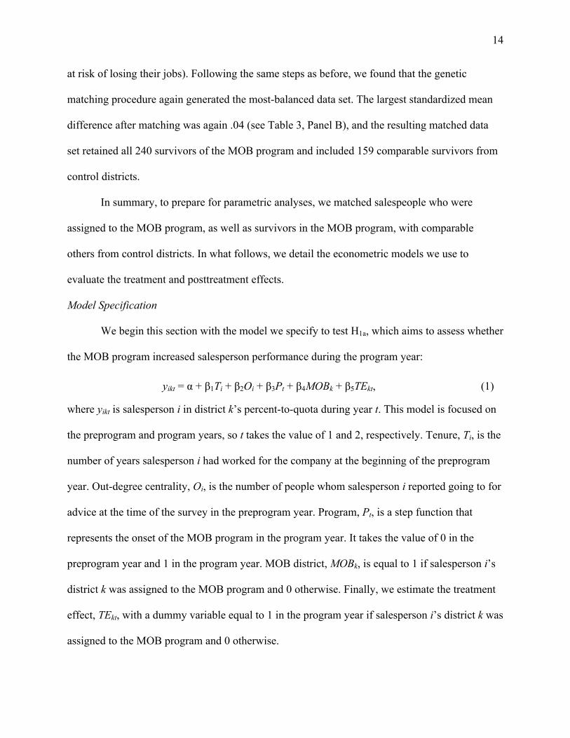
In Table 7 we also test H2c, the interaction between the posttreatment effect and the in-
degree centrality of a district’s replaced salesperson. If negative and significant, this coefficient
would indicate that survivors of the MOB program in districts that lost a central salesperson
decreased their performance in the postprogram year more than those in districts that lost a
salesperson on the periphery of the advice network. Indeed, this is the case (β = –.97, p < .01),
which offers support for H2c. Figure 3 shows that the average change in performance for
survivors in districts that lost a salesperson with an in-degree centrality of 3 was approximately
12 percentage points. The same statistic for survivors in districts that lost a salesperson with an
in-degree centrality of 0 was approximately 5 percentage points. We subsequently elaborate on
the implications of this finding and all other findings in the “Discussion” section.
----- Insert Figure 3 about here -----
Robustness Assessment
While our matching procedure achieved balance on observable variables, it is possible
that there are unobserved differences between the treatment and control groups. In other words,
we could have omitted variables in Equation 1 that may influence both the performance and
MOB district selection. The resulting correlation between the treatment effect and the error term
may lead to endogeneity. Many econometric techniques developed recently can potentially
address such endogenous concerns. We rely on Park and Gupta’s (2012) method, which models
the joint distribution of the endogenous regressor and the error term using a copula method.
Their model includes two important assumptions: the error is normally distributed, while the
endogenous regressor is not normally distributed. The nonnormality of an endogenous regressor

21
is required for model identification. The assumption of error normality is reasonable in most
empirical settings. As our endogenous regressor is binary, the assumption of nonnormality is also
satisfied. Therefore, Park and Gupta’s method is suitable in our context. We find that the MOB
program has a significant effect on performance (5.330, p < .01).
Discussion
In Study 1, we used a field-based quasi-experiment to test our hypotheses and examined
two phenomena. First, we observed that the MOB program significantly improved salespeople’s
performance. Second, we found that performance improvement was higher for salespeople who
had lower past performance and for salespeople who actively sought advice from their peers.
These results highlight the importance of having sticks in place, especially to motivate lower
performers.
The quasi-experiment of Study 1 lends itself to two limitations. First, it involved a single
firm implementing the MOB program and thus raises the issue of generalizability. Second, Study
1 cannot address the question whether vividness of the threat (i.e., having a replacement in sight)
exerts an increased effect on performance. Next, we present Study 2 to address these limitations.
STUDY 2: LAB EXPERIMENT
In Study 2, we design an experiment to (1) address the limitations of Study 1, (2)
replicate the central hypothesis to enhance the generalizability of the findings in Study 1, and (3)
compare the effectiveness of the MOB program with other forms of performance pressure:
displaying relative performance and firing the lowest-performing salesperson for not achieving
the quota.

22
Experiment Task
We chose a simple counting task for our experiment. The experimental task requires
counting the number of zeros in tables that consisted of 40 randomly ordered zeros and ones.
Prior studies have also used this task (e.g., Abeler et al. 2011). The advantages of this task are
threefold. First, it does not require any prior knowledge. Therefore, there is little scope for
unobserved heterogeneity among the participants. Second, little learning is possible during the
experiment. Third, the performance is easily measurable and highly correlated with the effort.
Therefore, the change in performance is directly attributable to change in the effort. Such real
effort tasks are increasingly used in experiments in various fields. The main advantage of using a
real effort task is the greater external validity of the experiment—exerting effort in the laboratory
task replicates the exertion of effort in the field (Gill and Prowse 2011). In each round, the
participant’s score is the number of tables in which the zeros were correctly counted.
Procedure and Sample
The experiment involved six rounds, with each round lasting for 2 minutes. In any round,
participants received a payment of $.70 for participation and a bonus payment of $.30 for
reaching or exceeding the target score of 15. We chose the split of 70:30 between the
participation payment and the bonus payment because this is the most common fixed and
variable pay ratio used in sales practice (SalesGlobe 2015). In addition, we chose 15 as the target
score from our pretest average. This ensured that the target score was realistic, with participants
likely to score both above and below the target score. The experimental sessions lasted for 20
minutes on average.
We had four experimental conditions: control condition (no performance pressure), Rank
condition (relative performance is displayed publicly), Fire condition, and MOB condition. In
both the Fire and the MOB conditions, if a participant was the lowest-performing person in his or

23
her group and did not meet the target, he or she was asked to leave after four rounds (i.e., could
not participate in the final two rounds). In addition, the MOB condition had a reserve participant
sitting next to each group who could potentially replace the participant with the lowest
performance who did not meet the target. In other words, the only difference between the Fire
and MOB conditions was the vividness of the threat: a reserve participant sitting next to each
group in the MOB condition.
We began by observing participants without any performance pressure in the first two
rounds. In other words, in all four conditions, participants could earn $.70 for participation and
$.30 for achieving the target, and there was no threat of being fired. This helped us establish the
baseline and ensured that there were no differences among the four experimental conditions.
Next, we assigned different conditions across the four experimental conditions and maintained
the same condition for two consecutive rounds (i.e., round three and four) within each
experimental condition: control, Rank, Fire, and MOB. Specifically, in the Fire and MOB
conditions, the participants were told that whoever scored the least and did not meet the
cumulative target score of 30 (each round target is 15) could no longer participate in the final
two rounds. Moreover, the MOB condition had additional participants in reserve who sat next to
each of the groups. By contrast, participants in the control and Rank conditions did not face any
threat of losing their position in the final two rounds. However, in the Rank condition, they were
able to see their peers’ scores. In the final two rounds, the participants did not face any
performance pressure (same as in the first two rounds).
One hundred eighty undergraduate students participated in the study. We randomly
assigned the participants to one of the four conditions (i.e., 45 participants in each condition) and

24
then further divided those in each condition into groups of five, resulting in nine groups in each
condition.
Results
In the first two rounds, the average score across the experimental conditions did not differ
(F(3, 354) = .16, n.s.). This finding provides confidence that randomization ensured that the
participants were similar across the experimental conditions.
In the third and fourth rounds, we found significant differences in mean performance
across the conditions (F(3, 354) = 50.46, p < .001; Wilks's λ = .700). To examine which of the
means are different, we performed the Tukey HSD (honest significant difference) test, which
allows comparison of means across multiple treatments. The results indicate that the MOB
condition outperformed the Fire condition (diff. in scores = 1.611, p < .001), which in turn
outperformed the Rank condition (diff. in scores = 1.955, p < .001). We found no difference in
performance between the Rank and control conditions (diff. in scores = .111, n.s.).
These results are consistent under a difference-in-differences specification as well.
Specifically, as Table 8 indicates, the treatment effect for the Fire condition is 1.967 (p < .0001)
and for the MOB condition is 3.344. The posttreatment effect for the Fire condition is –.881 (p <
.05), while the posttreatment effect for the MOB condition is –2.35 (p < .0001).
----- Insert Table 8 and Figure 4 about here -----
Based on the performance in the third and fourth rounds, we fired seven and three
participants in the Fire and MOB conditions, respectively. We replaced the three participants in
the MOB condition with the reserve participants in the final two rounds.

25
Discussion
The findings of Study 2 complement Study 1’s findings in several ways. First, we
replicated the findings of the main effect of MOB that received support in Study 1. Second, we
found that the threat of being fired motivated participants to increase their effort. Specifically,
participants’ performance in both the Fire and MOB conditions was higher than that in the
control and Rank conditions. Third, MOB had a greater effect on performance than simply firing
for poor performance. Importantly, this result shows that vividness of the threat (a bench player)
yields superior performance.
GENERAL DISCUSSION
One of the most common problems that sales managers face in the field today is how to
effectively motivate their sales force, especially the bottom performers. In order to shed light on
this important issue, we examined the role of sticks as an approach to better motivate
salespeople. Our research has taken a step in addressing this issue yielding specific managerial
actions that can be used to significantly impact the sales performance.
Research Implications
First, no prior study within the extant sales force literature has examined the role of
sticks. Past research on sales force motivation provides guidance on optimal incentive designs,
such as prize structure in sales contests and optimal structure of variable pay. However, research
has largely ignored the role of sticks in motivating the sales force. This is surprising because
companies heavily use sticks to motivate their sales force. Therefore, testing whether sticks are
effective is critical not only from a theoretical perspective but also from a practical viewpoint. To

26
that effect, our study introduces a novel form of stick: the MOB program. The results from Study
1 highlight the causal effect of the MOB program on salespeople’s performance. The MOB
program could have improved performance through two possible mechanisms: inducing greater
effort or honing selling skills. The pattern of the shifts in performance, rising immediately after
the introduction of the MOB program and dropping instantly in the month following its removal,
indicates that salespeople responded to the program by altering their effort. Moreover, the effect
of the MOB program was highest among the bottom performers. This implies that without some
form of stick in place, a segment of salespeople might not be putting in optimal levels of work.
This suggests using some form of stick along with carrots to manage the sales force.
Second, we contribute to the social network literature on sales force by examining the
impact of networks during punishments. The nascent literature examining salespeople’s social
networks indicates that salespeople with better connections have substantially higher
performance (Bolander et al. 2015). Our nuanced findings shed further light on the social
networks among the salespeople. First, our results suggest that salespeople’s connections,
operationalized as advice networks, help salespeople cope better during the MOB program.
Second, while previous research highlights mostly the positive benefits of these networks, we
demonstrate that the replacement of a central salesperson can be detrimental to the performance
of other salespeople.
Third, in Study 2, we compared the various forms of sticks prevalent in practice.
Specifically, we compared three programs: displaying relative performance (e.g., scoreboards),
firing for poor performance, and the MOB program. The last two programs are identical except
that an extra participant was waiting to take a participant’s position in the MOB program. The
results reveal that while displaying relative performance does not yield superior performance, job

27
insecurity arising from the other two programs enhances performance. More important, we find
that performance is higher in the presence of a replacement in sight. In other words, the vividness
of the job threat has an effect on performance.
Fourth, we contribute to the nascent literature on incentives and punishments in allied
fields. While researchers have devoted significant effort in the past half century to examine the
role of incentives, the interaction between incentives and punishments has gained attention only
in the past decade. For example, Fehr and Schmidt (2007) are among the first to investigate how
adding a stick to the carrot affects performance. Surprisingly, they find that the combination of
carrots and sticks does not improve performance. They reason that under an explicit threat of a
punishment, which may be viewed as hostile, people reciprocate by choosing a lower level of
effort. Our results from Study 1 and Study 2 contradict this finding by showing that performance
significantly improves when a punishment is added to the existing incentives. The difference in
the level of punishment could explain this discrepancy: the punishment in our studies was
stronger than the one Fehr and Schmidt use. Specifically, whereas in Study 1 (Study 2), the
salespeople (participants) may lose their employment (ability to participate in the final two
rounds), the participants in Fehr and Schmidt’s experiment faced much milder punishment in the
form of a fine. Therefore, we argue that when the level of punishment is reasonably high,
punishment combined with incentives leads to superior performance. Moreover, to the best of
our knowledge, our study is the first comprehensive field experiment to examine the role of
sticks.
Managerial Implications
Sales managers face two persistent challenges in garnering superior performance from
their salespeople. First, they often find it difficult to motivate the bottom performers, who might

28
be dragging down the performance of the entire sales force. Second, they often do not fire a
poorly performing salesperson because of costs such as finding a replacement, training the new
hire, and leaving territories vacant for a long time. Our findings indicate that a stick program
such as MOB can effectively overcome these challenges. Specifically, during the MOB program
we observed the highest improvement in performance among the bottom performers. Moreover,
hiring bench salespeople makes it easier for managers in their tradeoff between retaining chronic
low performers and enduring vacant sales territories. We make three recommendations based on
our findings.
We recommend that firms use some kind a stick to motivate their sales force. Both our
studies demonstrate the applicability and superiority of the combination of punishment and
incentives to using pure incentives. Moreover, we particularly recommend that firms that have
chronic underperforming salespeople rely on sticks. In our field experiment, a significant portion
of salespeople were suspected of underachieving relative to the market potential, which allowed
for the increase in performance that we observed during the program year in MOB districts. This
performance increase is necessary though to offset the cost of hiring and training new
salespeople.
When a company has a disproportionate number of underperforming salespeople, the
cause is usually due to sales managers’ reluctance to face a difficult transition period of
recruiting and training a new salesperson. This is understandable, as transitions generally lead to
a 13.2%–17.6% annual loss in sales (Shi et al. 2017). Moreover, peers and subordinates may not
perceive a manager firing underperforming salespeople favorably. For example, in their lab
experiment, Fehr and Schmidt (2007) show that the majority of the participants acting as
managers preferred to offer a simple incentive contract to the option that combined both

29
incentives and punishments. To this end, the MOB program helps managers overcome these
obstacles. It ensures that turnover costs, such as those associated with recruitment and selection,
training, and territory vacancy, are decoupled from sales managers’ dismissal decisions as
reserve salespeople are trained during the program so that they can be put into the starting lineup
seamlessly. In addition, it imposes a formal rule for dismissal to guard against sales managers’
aversion to enforcing corrective action. In other words, as top management is instrumental in
implementing the MOB program, sales managers find it easier to let go of the underperformers.
Finally although many suggest that salespeople devolve into ruthless competition for
resources when job threats arise, our data imply that the opposite may be true, as salespeople
who seek advice from their peers are able to enhance their performance and fend off the threat
from the bench. Therefore, social cohesion seems to be an important factor for managers to
consider when deciding whether to enact a program such as the one studied herein.
Limitations and Further Research
As with all studies, the current research should be interpreted in light of a few limitations.
Although the MOB program is easily generalizable to other contexts, further research could
examine other types of benches (e.g., pools of qualified applicants, temporary employees). Our
research examines only salespeople’s performance as a dependent variable. Although
performance is a crucial variable from a managerial perspective, examining other dependent
variables (e.g., job satisfaction, turnover, and organizational culture) is essential for knowledge
in this area to develop. We use the overall advice network of a salesperson. Additional research
could examine frequency and type of advice network. Future research could examine whether the
bench players outperform new hires in the control districts and provide further information on
the effectiveness of such programs.

30
References
Abeler, Johannes, Armin Falk, Lorenz Goette, and David Huffman (2011), "Reference Points and Effort Provision," American Economic Review, 101 (2), 470-92. Ahearne, Michael, Adam Rapp, Douglas E. Hughes, and Rupinder Jindal (2010), "Managing Sales Force Product Perceptions and Control Systems in the Success of New Product Introductions," Journal of Marketing Research, 47 (4), 764-76. Avery, Jill, Thomas J. Steenburgh, John Deighton, and Mary Caravella (2012), "Adding Bricks to Clicks: Predicting the Patterns of Cross-Channel Elasticities over Time," Journal of Marketing, 76 (3), 96–111. Banerjee, Ranjan, Mark Bergen, Shantanu Dutta, and Sourav Ray (2012), "Applications of Agency Theory in B2B Marketing: Review and Future Directions," in Handbook of Business-to-Business Marketing, Gary L. Lilien and Rajdeep Grewal, eds. Cheltenham: Edward Elgar Publishing, 41-53. Basu, Amiya K., Rajiv Lal, Venkataraman Srinivasan, and Richard Staelin (1985), "Salesforce Compensation Plans: An Agency Theoretic Perspective," Marketing Science, 4 (4), 267-91. Bolander, Willy, Cinthia B. Satornino, Douglas E. Hughes, and Gerald R. Ferris (2015), "Social Networks Within Sales Organizations: Their Development and Importance for Salesperson Performance," Journal of Marketing, 79 (6), 1-16. Brockner, Joel, Jeff Greenberg, Audrey Brockner, Jenny Bortz, Jeanette Davy, and Carolyn Carter (1986), "Layoffs, Equity Theory, and Work Performance: Further Evidence of the Impact of Survivor Guilt," Academy of Management Journal, 29 (2), 373–84. Brockner, Joel, Steven Grover, Thomas F. Reed, and Rocki Lee Dewitt (1992), "Layoffs, Job Insecurity, and Survivors' Work Effort: Evidence of an Inverted-U Relationship," Academy of Management Journal, 35 (2), 413–25. Challagalla, Goutam N., and Tasadduq A. Shervani (1996), "Dimensions and Types of Supervisory Control: Effects on Salesperson Performance and Satisfaction." The Journal of Marketing, 60 (1), 89-105. Churchill, Gilbert A., Jr., Neil M. Ford, Steven W. Hartley, and Orville C. Walker Jr. (1985), "The Determinants of Salesperson Performance: A Meta-Analysis," Journal of Marketing Research, 22 (May), 103–18. Chung, Doug J., Thomas Steenburgh, and K. Sudhir (2013), "Do Bonuses Enhance Sales Productivity? A Dynamic Structural Analysis of Bonus-Based Compensation Plans," Marketing Science, 33 (2), 165-87.

31
Chung, Doug J., and Das Narayandas (2015), "Incentives Versus Reciprocity: Insights From A Field Experiment," Journal of Marketing Research, In-Press. Coughlan, Anne T. and Chakravarthi Narasimhan (1992), "An Empirical Analysis of Sales-Force Compensation Plans," Journal of Business, 65 (1), 93-121. Cron, William L., Alan J. Dubinsky, and Ronald E. Michaels (1988), "The Influence of Career Stages on Components of Salesperson Motivation," Journal of Marketing, 52 (1), 78–92. Darmon, Rene Y. (1990), "Identifying Sources of Turnover Costs: A Segmental Approach,” Journal of Marketing, 54 (2), 46-56. Diamond, Alexis and Jasjeet S. Sekhon (2013), "Genetic Matching for Estimating Causal Effects: A General Multivariate Matching Method for Achieving Balance in Observational Studies," Review of Economics and Statistics, 95 (3), 932–45. Dickinson, David L. (2001), "The Carrot vs. the Stick in Work Team Motivation," Experimental Economics, 4 (1), 107-24. Fehr, Ernst and Klaus M. Schmidt (2007), "Adding a Stick to the Carrot? The Interaction of Bonuses and Fines," American Economic Review, 97 (2), 177-81. Gilboa, Simona, Arie Shirom, Yitzhak Fried, and Cary Cooper (2008), "A Meta-Analysis of Work Demand Stressors and Job Performance: Examining Main and Moderating Effects," Personnel Psychology, 61 (2), 227–71. Gill, David, and Victoria L. Prowse (2011), "A Novel Computerized Real Effort Task Based on Sliders," working paper, Department of Economics, Purdue University. Grote, Richard C. (2005), Forced Ranking: Making Performance Management Work. Cambridge, MA: Harvard Business Press. Ho, Daniel E., Kosuke Imai, Gary King, and Elizabeth A. Stuart (2007), "Matching as Nonparametric Preprocessing for Reducing Model Dependence in Parametric Causal Inference," Political Analysis, 15 (3), 199–236. Ho, Daniel E., Kosuke Imai, Gary King, and Elizabeth Stuart (2011), "MatchIt: Nonparametric Preprocessing for Parametric Causal Inference," Journal of Statistical Software, 42, 1–28. Kishore, Sunil, Raghunath Singh Rao, Om Narasimhan, and George John (2013), "Bonuses versus Commissions: A Field Study," Journal of Marketing Research, 50 (3), 317-333. Koenker, Roger (2005), Quantile Regression. Cambridge, UK: Cambridge University Press. Kumar, V., Sarang Sunder, and Robert P. Leone (2014), "Measuring and Managing a Salesperson's Future Value to the Firm," Journal of Marketing Research, 51 (5), 591-608.

32
Lim, Noah, Michael J. Ahearne, and Sung H. Ham (2009), "Designing Sales Contests: Does the Prize Structure Matter?" Journal of Marketing Research, 46 (3), 356-71. Lo, Desmond, Mrinal Ghosh, and Francine Lafontaine (2011), "The Incentive and Selection Roles of Sales Force Compensation Contracts," Journal of Marketing Research, 48 (4), 781- 98. Miao, C. Fred, and Kenneth R. Evans (2013), "The Interactive Effects of Sales Control Systems on Salesperson Performance: A Job Demands–Resources Perspective," Journal of the Academy of Marketing Science, 41 (1),73-90. Misra, Sanjog and Harikesh S. Nair (2011), "A Structural Model of Sales-Force Compensation Dynamics: Estimation and Field Implementation," Quantitative Marketing and Economics, 9 (3), 211-57. Park, Sungho and Sachin Gupta (2012), "Handling Endogenous Regressors by Joint Estimation Using Copulas," Marketing Science, 31 (4), 567-86. Probst, Tahira M. (2002), "Layoffs and Tradeoffs: Production, Quality, and Safety Demands Under the Threat of Job Loss," Journal of Occupational Health Psychology, 7 (3), 211-220. SalesGlobe (2015), "What's So Great About Pay Mix?" (accessed May 22, 2017), [available at http://salesglobe.com/blog/whats-so-great-about-pay-mix]. Scott, John (2012), Social Network Analysis. Thousand Oaks, CA: Sage Publications. Scullen, Steven E., Paul K. Bergey, and Lynda Aiman-Smith (2005), "Forced Distribution Rating Systems and the Improvement of Workforce Potential: A Baseline Simulation," Personnel Psychology, 58 (1), 1–32. Shi, Huanhuan, Shrihari Sridhar, Rajdeep Grewal, and Gary Lilien. "Sales Representative Departures and Customer Reassignment Strategies in Business-to-Business Markets," Journal of Marketing, 81 (2), 25-44. Smith, Benson (2012), "When to Say, You're Fired!," accessed May 25, 2017, [available at http://businessjournal.gallup.com/content19660/when-to-say-youre-fired.aspx] Smith, Edward Bishop, Tanya Menon, and Leigh Thompson (2012), "Status Differences in the Cognitive Activation of Social Networks," Organization Science, 23 (1), 67-82. Steenburgh, Thomas J. (2008), "Effort or Timing: The Effect of Lump-Sum Bonuses," QME, 6 (3), 235–56. Vroom, Victor (1964), Work and motivation. New York: Wiley, 1964.

33
Walker Jr, Orville C., Gilbert A. Churchill Jr, and Neil M. Ford (1977), "Motivation and Performance in Industrial Selling: Present Knowledge and Needed Research." Journal of Marketing Research, 156-168. Welch, Jack, and John A. Byrne (2003), "Jack: Straight from the gut", Warner Books, New York, NY. Zoltners, Andris A., Prabhakant Sinha, and Sally E. Lorimer (2006), "Match Your Sales Force Structure to Your Business Life Cycle," Harvard Business Review, 84 (7/8), 80-89.

34
TABLE 1 Sales Force Research on Rewards and Punishments
Outcome controls Behavioral controls
Rewards
(Carrots)
• Bonuses motivate salespeople to work harder
rather than play timing games (Steenburgh 2008)
• Firms design their incentive plans to both select
salespeople and provide them with the right level
of incentives (Lo, Ghosh, and Lafontaine 2011)
• Commission plans outperform bonus plans
(Kishore et al. 2013)
• Overachievement commissions help sustain the
high productivity of the top performers, and
quarterly bonuses help improve performance of
the bottom performers (Chung, Steenburgh, and
Sudhir 2014)
• Unconditional bonuses in the form of reciprocity
enhance performance (Chung and Narayandas
2015)
• Behavioral controls strengthen the
effect of outcome controls on effort
(Miao and Evans 2012)
• Behavioral control systems negatively
affect new product sales (Ahearne et
al. 2010)
Punishment
(Sticks)
• Current Research
• Behavioral punishments do not
enhance salesperson performance
(Challagalla and Shervani 1996)

35
TABLE 2 Descriptive Statistics for the Matching Variables Grouped by District Type
MOB Districts M (SD)
Control Districts M (SD)
All Districts M (SD)
Tenure 9.51 9.91 9.74 (6.20) (6.51) (6.39) District size 5.15 5.32 5.25 (1.19) (1.33) (1.28) Preprogram performance (2 years before) 99.63 99.31 99.44 (9.86) (9.79) (9.82) Preprogram performance (1 year before) 96.45 96.37 96.40 (7.99) (8.16) (8.09) Variability in preprogram performance .05 .05 .05 (.03) (.03) (.03) Out-degree centrality .75 .50 .60 (.83) (.68) (.75) Number of salespeople 286 413 699 Number of districts 58 82 140 Number of salespeople replaced 46 0 46

36
TABLE 3 Matching Algorithms
A: Balance Achieved by Various Matching Algorithms between Salespeople in Treatment and Control Districts
Standardized Mean Differences by Matching Algorithm Matching Variable Unmatched Nearest Optimal Subclass Full Genetic Tenure –.06 –.02 .02 .08 –.04 .04 District size –.14 –.01 –.01 .05 –.15 .01 Preprogram performance (2 years before) .03 –.04 –.01 .08 –.08 .00 Preprogram performance (1 year before) .01 –.04 .00 .07 –.08 –.01 Variability in preprogram performance –.06 .01 –.01 .07 –.02 .01 Out-degree centrality .30 .17 .14 .06 –.06 .00 Number of salespeople in MOB districts 286 286 286 286 286 286 Number of salespeople in control districts 413 286 286 413 413 188
B: Balance Achieved by Various Matching Algorithms between Survivors in Treatment and Control Districts
Standardized Mean Differences by Matching Algorithm Matching Variable Unmatched Nearest Optimal Subclass Full Genetic Tenure –.01 .00 .07 .10 .04 –.01 District size –.11 .00 .03 .05 –.03 .04 Preprogram performance (2 years before) .19 .08 .02 .05 .08 –.01 Preprogram performance (1 year before) .16 .09 .02 .04 .10 –.04 Variability in preprogram performance –.06 –.05 .00 .03 .03 .03 Out-degree centrality .30 .07 .11 .04 –.04 .01 Number of salespeople in MOB districts 240 240 240 240 240 240 Number of salespeople in control districts 413 240 240 413 413 159

37
TABLE 4 Difference-in-Differences Analysis (Matched Sample)
A: All Matched Salespeople Preprogram Year
Performance Program Year Performance
Difference (Program – Preprogram)
MOB 96.45 101.39 4.94*** (.47) (.49) (.68) Control 96.56 97.42 .86 (.56) (.80) (.97) Difference −.11 3.97*** 4.07*** (MOB – Control) (.73) (.93) (1.15)
Notes: Standard errors are in parentheses; unequal variances are assumed for the t-tests; the t-tests and difference-in-differences estimate are weighted according to the weights provided by the genetic matching procedure; the number of salespeople in the matched data set is 474. *** p < .001.
B: Preprogram Year Last-Place Performers Preprogram Year
Performance Program Year Performance
Difference (Program – Preprogram)
MOB 87.27 96.44 9.17*** (.80) (.91) (1.21) Control 88.29 88.01 −.28 (.96) (1.64) (1.90) Difference −1.02 8.43*** 9.45*** (MOB – Control) (1.28) (1.94) (2.18)
Notes: Standard errors are in parentheses; unequal variances are assumed for the t-tests; the t-tests and the difference-in-differences estimate are weighted according to the weights provided by the genetic matching procedure; the number of preprogram year last-place performers in the matched data set is 94. *** p < .001.
C: Preprogram Year Second-to-Last-Place Performers Preprogram Year
Performance Program Year Performance
Difference (Program – Preprogram)
MOB 92.95 100.17 7.22*** (.59) (.94) (1.11) Control 92.75 94.25 1.50 (.63) (1.44) (1.57) Difference .20 5.92** 5.71** (MOB – Control) (.86) (1.70) (1.85)
Notes: Standard errors are in parentheses; unequal variances are assumed for the t-tests; the t-tests and the difference-in-differences estimate are weighted according to the weights provided by the genetic matching procedure; the number of preprogram year second-to-last-place performers in the matched data set is 98. *** p < .001; ** p < .01.
D: Preprogram Year First-Place Performers Preprogram Year
Performance Program Year Performance
Difference (Program – Preprogram)
MOB 105.61 106.45 .84 (.81) (.94) (1.24) Control 104.61 103.99 −.62 (1.34) (1.81) (2.25) Difference 1.00 2.46 1.46 (MOB – Control) (1.56) (2.03) (2.38)
Notes: Standard errors are in parentheses; unequal variances are assumed for the t-tests; the t-tests and the difference-in-differences estimate are weighted according to the weights provided by the genetic matching procedure; the number of preprogram year first-place performers in the matched data set is 96.

38
TABLE 5 The Treatment Effect of the MOB Program on Performance for the Sample of
Matched Salespeople Dependent Variable: Performance Intercept 96.67*** (.60) Tenure .35 (.33) Out-degree centrality −1.51*** (.40) Program .86 (.63) MOB district −.12 (.77) Treatment effect 3.97*** (.80) Treatment effect × out-degree centrality 1.60*** (.46)
F-value 13.98*** R2 .08
Notes: The dependent variable is performance during the preprogram and program years; we standardized tenure and out-degree centrality before estimating the model for interpretability purposes; the number of observations is 948; the number of salespeople is 474 (286 from MOB districts and 188 from control districts); standard errors are in parentheses and clustered at the district level. *** p < .001.

39
TABLE 6 Change in Rank from the Preprogram Year to the Program Year for Preprogram Year
Last-Place, Second-to-Last-Place, and First-Place Performers by Condition Rank Δ
Preprogram Rank Down One Stayed
the Same Up One or Two
Up Three or More
Last Place MOB N/A 43% 40% 17% Control N/A 54% 37% 9% Second-to-Last Place MOB 26% 17% 43% 14% Control 20% 44% 24% 12%
Rank Δ
Preprogram Rank Up One Stayed
the Same Down One
or Two Down Three
or More First Place MOB N/A 43% 43% 14% Control N/A 53% 30% 17% Notes: Across the rows of this weighted frequency table, the matched salespeople are grouped by condition (i.e., MOB or control) and within-district rank in the preprogram year (i.e., last place, second-to-last place, or first place). With varying degrees and directions of rank changes in the columns, the cells indicate whether, in what direction, and how much matched salespeople of different types changed ranks from the preprogram year to the program year.

40
TABLE 7 The Treatment Effect and Posttreatment Effect of the MOB Program on Performance for
the Sample of Matched Survivors Dependent Variable: Performance Intercept 97.86*** (.58) Tenure −.10 (.28) Out-degree centrality −1.08** (.34) Program .55 (.63) Postprogram −1.00 (.94) MOB district .76 (.77) Replaced district −1.18 (.85) In-degree centrality of a district’s replaced salesperson −.22 (.38) Treatment effect 5.27*** (.84) Posttreatment effect −5.00*** (1.15) Treatment effect × out-degree centrality .89* (.41) Posttreatment effect × replaced district .64 (.73) Posttreatment effect × in-degree centrality of a district’s replaced salesperson −.97** (.39)
F-value 12.32*** R2 .11
Notes: The dependent variable is performance during the preprogram, program, and postprogram years; we standardized tenure, out-degree centrality, and in-degree centrality of a district’s replaced salesperson before estimating the model for interpretability purposes; the number of observations is 1,197; the number of survivors is 399 (240 from MOB districts and 159 from control districts); standard errors are in parentheses and clustered at the district level. *** p < .001; ** p < .01; * p < .05.

41
TABLE 8 Study 2: The Treatment Effect and Posttreatment Effects of Rank, Fire, and MOB
Programs DV: Participant’s Score Intercept 14.32*** (.38) Rank .19 (.42) Fire .04 (.52) MOB .26 (.54) Program .22 (.45) Postprogram .10 (.37) Treatment Effects
Rank -.13 (.65)
Fire 1.97*** (.49)
MOB 3.34*** (.52) Posttreatment Effects
Rank .61 (.66)
Fire -.88* (.41)
MOB -2.35*** (.48)
Notes: Clustered standard errors are in parentheses. * p < .05, ** p < .01, *** p < .001.

42
Notes: The lines display salespeople’s and survivors’ average monthly performance, weighted according to the weights generated by the genetic matching procedure. During the program year, separation between the dashed and solid lines represents the treatment effect. During the postprogram year, lack of separation between the two lines represents the posttreatment effect.
Preprogram Year Program Year
80%
90%
100%
110%
1 6 12 18 24Month
Perf
orm
ance
Condition Control MOB Program
FIGURE 1AThe Treatment Effect for the Sample of Matched Salespeople by Month
Preprogram Year Program Year Postprogram Year
80%
90%
100%
110%
1 6 12 18 24 30 36Month
Perf
orm
ance
Condition Control MOB Program
FIGURE 1BThe Treatment and Posttreatment Effects for the Sample of Matched Survivors by Month

43
Notes: The points display the treatment effect and the posttreatment effect of the MOB program for nine deciles of the company’s performance distribution. The first and ninth deciles pertain to the company’s lowest and highest performers, respectively. The error bars represent 95% confidence intervals of the coefficients displayed as points.
●
●
● ● ● ● ●
●
●
−5%
0%
5%
10%
15%
FirstDecile
SecondDecile
ThirdDecile
FourthDecile
FifthDecile
SixthDecile
SeventhDecile
EighthDecile
NinthDecile
Performance Decile
Trea
tmen
t Effe
ctFIGURE 2A
The Treatment Effect for the Sample of Matched Salespeople by Decile
●
●●
● ●
●●
●
●
−15%
−10%
−5%
0%
5%
FirstDecile
SecondDecile
ThirdDecile
FourthDecile
FifthDecile
SixthDecile
SeventhDecile
EighthDecile
NinthDecile
Performance Decile
Post
trea
tmen
t Effe
ct
FIGURE 2BThe Posttreatment Effect for the Sample of Matched Survivors by Decile
●
●
● ●●
●
●●
●
−5%
0%
5%
10%
15%
FirstDecile
SecondDecile
ThirdDecile
FourthDecile
FifthDecile
SixthDecile
SeventhDecile
EighthDecile
NinthDecile
Performance Decile
Trea
tmen
t Effe
ct
FIGURE 2CThe Treatment Effect for the Sample of Matched Survivors by Decile
44
Notes: The columns display average changes in performance (from the program year to the postprogram year) for survivors of the MOB program working in districts that replaced a salesperson. These average changes in performance are grouped according to how central a district’s replaced salesperson was in the district’s advice network, with centrality measured as the number of salespeople that reported going to the replaced salesperson for advice (i.e., in-degree centrality). The error bars represent standard errors.
−15%
−10%
−5%
0%
0 1 2 3Indegree Centrality of a District's Replaced Salesperson
Cha
nge
in P
erfo
rman
ceFIGURE 3
The Average Change in Performance of a District's Survivors bythe Indegree Centrality of a District's Replaced Salesperson

45
●
●●●
●●●●
●●
●
●
●
●
●
●
●
●●
●
●
●
●●
Preprogram Rounds Program Rounds Postprogram Rounds
11
13
15
17
19
1 2 3 4 5 6Round
Perf
orm
ance
Condition Control Rank Fire MOB Program
FIGURE 4The Treatment and Posttreatment Effects for Participants of Study 2 by Round

46
Web Appendix
Genetic Matching Algorithm
Matching has become an important tool in many fields, including marketing. One of the popular
matching techniques is propensity score matching. Matching on a correctly specified propensity score
achieves covariate balance – the treatment and control groups have the same joint distribution of observed
covariates. The balance of covariates between the treatment and control groups allows one to make causal
inferences.
Rosenbaum and Rubin (1984) recommend that the specification of propensity score should be revised
until covariate balance is maximized. However, the process of iteratively modifying the propensity score
to minimize imbalance is challenging. Genetic matching eliminates the manual process of checking the
propensity score by using an evolutionary search algorithm to iteratively check and maximize the balance
between observed covariates. In fact, both propensity score matching and matching based on Mahalanobis
distance are limiting cases of Genetic Matching (Diamond and Sekhon 2013).