Copyright © 2008 by Gregory M. Barron and Stephen Leider

Working papers are in draft form. This working paper is distributed for purposes of comment and discussion only. It may not be reproduced without permission of the copyright holder. Copies of working papers are available from the author.

Making the Gambler’s Fallacy disappear: The role of experience Gregory M. Barron Stephen Leider

Working Paper

09-029

Making the Gambler’s Fallacy disappear:

The role of experience†

Greg Barron* and Stephen Leider

Harvard Business School and Department of Economics

*Address correspondence to: Greg Barron, Harvard Business School, Boston MA, 02163, Email: gbarron@hbs.edu †Acknowledgements: We are grateful to the National Science Foundation and the Sperry Fund for financial support (to S. Leider). We have benefited from discussions with and comments from Ido Erev, Max Bazerman, and workshop participants at Unravelling Decisions from Experience, University College London. All remaining errors are our own.

Making the Gambler’s Fallacy disappear: The role of experience

Abstract:

Recent papers have demonstrated that the way people acquire information about a decision problem, by experience or by abstract description, can affect their behavior. We examine the role of experience over time in the emergence of the Gambler’s Fallacy in binary prediction tasks. Theories of the Gambler’s Fallacy and models of binary prediction suggest that recency bias, elicited by experience over time, may be necessary for the fallacy to emerge. Experiment 1 compares a condition where participants sequentially predict the colored outcomes of a roulette wheel with a condition where the wheel’s past outcomes are presented all at once. Subjects are yoked so that the same history of outcomes is observed in both conditions. The results reveals a tendency towards negative recency when outcomes are experienced that disappears when the same outcomes are presented all at once. Experiment 2 examines a boundary condition where outcomes are presented sequentially in an automatic fashion without intervening predictions. Here too, the Gambler’s Fallacy emerges suggesting that it is the mere presentation of information over time that gives rise to the bias. Implications are discussed.

Making the Gambler’s Fallacy disappear: The role of experience

Consider an expecting mother about to give birth to her 11th child. She currently has 5

boys and 5 girls but the last 4 births have been girls. Understandably she feels strongly that a boy

is long “overdue” (i.e. the Gambler’s Fallacy). If the mother-to-be describes to her new

pediatrician the birth order of her children (MMFMMMFFFF), should we expect the pediatrician

to hold the same belief? Imagine now the roulette player at a Vegas casino who has just

experienced 5 red outcomes in a row. Even a decision scientist would be hard put not to feel that

a black outcome is now likely. But what if the player had just arrived at the table and seen the

following history of 10 red (R) and 10 black (B) outcomes displayed above the table

(BBRBBBRBBRRRBBBRRRRR). Should she exhibit the Gambler’s Fallacy as strongly as the

gambler who just witnessed the revelation of those outcomes over time?

In this paper we ask the question: does the way we acquire information, by sequential

experience or by simultaneous description, play a critical role in the emergence of the Gambler’s

Fallacy in a binary prediction task? The question is an interesting one since several recent papers

on decisions from experience and descriptions suggest that the way people acquire information,

by personal experience like the mom-to-be or by description like the pediatrician, can have a

significant effect on choice behavior. Binary prediction tasks, like betting on red or black, are a

natural decision context to explore for similar effects. By examining this question we hope to

both extend the literature on decisions from experience and description, and to deepen our

understanding of the underlying cause of Gambler’s Fallacy by identifying some of its boundary

conditions.

The Gambler’s Fallacy, often attributed to Laplace’s essay of 17961 and the experimental

work of Murray Jarvik (1951), refers to the belief that runs of one binary outcome will be

balanced by the opposite outcome. Moreover, the longer the run, the stronger the belief that the

opposite outcome is due to appear. Many studies have explored this effect and found it robust in

different experimental paradigms such as prediction of binary outcomes, generation of random

1" I have seen men, ardently desirous of having a son, who could learn only with anxiety of the births of boys in the month when they expected to become fathers. Imagining that the ratio of these births to those of girls ought to be the same at the end of each month, they judged that the boys already born would render more probable the births next of girls."(from A Philosophical Essay on Probabilities by Laplace [1951, p.162])

sequences and identification of sequences as random (e.g. Budescu, 1987; Bar-Hillel &

Wagenaar, 1991, for a review, see Lee, 1971, chapter 6).

Our suggestion that the emergence of the Gambler’s Fallacy may be affected by how

information about past outcomes is presented is motivated by recent work on decisions from

experience and decisions from description. In decisions from description, outcome distributions

are described abstractly, for example a choice between $3 with certainty and a lottery providing

$32 with probability 0.1 and $0 otherwise. An experience-based choice between the same two

options would be based on outcomes incurred in the past from repeated draws from the two

distributions. Alternatively, samples may be drawn and merely observed (without incurring any

financial gain or loss) after which an individual chooses a single distribution to receive an

outcome draw from (see Weber, Blais & Shafir, 2004). In both cases the decision maker has to

rely solely on past outcomes to make her decision. Barron & Erev (20003) demonstrate that the

deviations from maximization that one observes in choices between lotteries depend critically on

how the information was acquired (i.e. through a description or through experience). Notably,

while small probabilities are overweighted in decisions from description (Kahneman & Tversky,

1979; Tversky & Kahneman, 1992) they tend to be underweighted in decisions form experience

(Erev & Barron, 2005; Hertwig, Barron, Elke & Erev, 2004; Fox & Hadar, 2006; Barron, Ursino

& Yechiam, 2008).

Related research has shown that experience can lead to suboptimal responding in a binary

prediction task (Newell & Rakow, 2007). In predicting the binary outcome of a dice throw with

four sides of the die in one color and two sides in a second color, participants gave the

maximizing prediction more often when the problem was described abstractly, without observing

any actual outcomes. Experience, on the other hand, was found to lead to behaviors such as

probability matching that are more “representative” of the process generating the outcomes.

Clearly, one would not expect the Gambler’s Fallacy to emerge based on an abstract

description of a random process. Having been told only that a roulette wheel’s red and black

outcomes are equally likely, there is no reason to believe one outcome is more likely to appear

next. However, it is less clear when predictions are based on a sequence of past outcomes

presented all at once. In typical studies of the Gambler’s Fallacy subjects experience, and

predict, series of binary outcomes one at a time. We are not aware of published studies where

predictions are based on full sequences of past outcomes (as in the example where a gambler

approaches a roulette table and observes the table’s history of outcomes). Combining relevant

characteristics of both experience and a description, evaluating and choosing based on a full

sequence is cognitively very different then the task of sequential, one-at-a-time, prediction.

This very distinction was the focus of Hogarth and Einhorn’s (1992) paper on beliefs and

order effects. They undertook a meta-analysis of order effects in studies employing simple tasks

with short (2-12 items) series. They find that recency occurred in every study (16/16) where

subjects express their beliefs after integrating each piece of evidence in a given sequence step-

by-step. However, in studies where subjects reported opinions only after all the information has

been presented, recency was observed much less often (8 out of 27 studies). To organize the

pattern of order effects, Hogarth and Einhorn propose a general model of information processing

and belief adjustment. For our purposes the key feature is the distinction between Step-by-step

and End-of-sequence information processing.2 Hogarth and Einhorn argue that Step-by-step

tasks (i.e. tasks that ask for a response after each piece of evidence) necessitate Step-by-step

thinking, while End-of-sequence tasks (i.e. a response is only needed after all evidence has been

collected) will tend towards End-of-sequence processing (unless long and/or complex sequences

of evidence necessitate Step-by-step processing due to memory constraints). As the outcomes in

our experiment will be simple and the sequence lengths short, we can reasonably expect that

subjects will use an End-of-sequence when presented with a simultaneous complete description

of the previous outcomes. Critically, Hogarth and Einhorn argue that the moving average

calculation in Step-by-step processing will display recency, i.e. increased sensitivity to the last

few outcomes, while the holistic End-of-sequence process will not have recency (and in fact may

have primacy, i.e. sensitivity to the initial outcome, due to initial anchoring with a single

adjustment for all the evidence).

We argue, therefore, that applying this adjustment model to either of the leading

accounts for the mechanism behind the Gambler’s Fallacy (identified by Ayton and Fischer

2004) will naturally imply that the recency bias caused by the sequential presentation is critical 2 Hogarth and Einhorn also distinguish between tasks that call for evaluation (assessing if a hypothesis is true or false) and tasks that call for estimation (constructing some form of a “moving average”). In their model this serves to establish whether the new piece of evidence is compared to a constant reference point (e.g. zero, where an outcome is positive if it supports the hypothesis, and negative if it contradicts) or to the current belief (e.g. last period’s posterior for the average). All of our treatments use prediction tasks, which are best classified as estimation tasks. Notably, however, other studies of the Gambler’s Fallacy have used identification tasks, which may be considered evaluation tasks in Hogarth’s framework.

for the presence of the Gambler’s Fallacy in binary prediction tasks. Estes (1964) presented the

first major account of the Gambler’s Fallacy, suggesting that subjects bring into the lab a folk

intuition that, in general, random outcomes will act like sampling without replacement, based on

their experience in the outside world, where such behavior is often the norm. For example, the

100th car in a train portends the caboose with greater likelihood than the third car (Pinker, 1997).

When finite populations are sampled without replacement astute observers should commit the

Gambler’s Fallacy. The Gambler’s Fallacy bias can occur, then, when a sequence of the same

outcome “uses up” those outcomes from the overall random process. This effect should be more

extreme when individuals focus on the smaller subsequence of the most recent results (since

smaller sequences are more volatile and thus more likely to deviate from the expected

frequencies). For example, suppose a gambler betting on roulette has a mental model of drawing

without replacement from 15 red outcomes and 15 black outcomes. When faced with the

sequence BBRBBBRBBRRRBBBRRRRR, if recency causes him to focus on the last 5

outcomes he may believe that Black has a 60% probability of occurring (since there are 10 red

and 15 black “left” from the initial 30 outcomes). If, however, he considers all 20 observed

outcomes, he correctly believes that red and black are equally likely (5 red and 5 black are

“left”).

The second proposed model is the representativeness heuristic (Kahneman & Tversky,

1972), where individuals expect that the characteristics of populations are similarly represented

at a local level as well. Thus if the likelihood of giving birth to boys and girls is same, the same

number of boys and girls is expected in any given small sample of births. Consequently, people

expect runs of the same outcome to be less likely than they are. Recency arguably plays a

critical role in the process of determining exactly what is “local” (i.e. the size and serial location

of the sample that is expected to be representative of the population). If the recent series of four

daughters is particularly salient to the mother, she may feel that the last four outcomes do not

reflect the overall equal proportions of males and females; thus she may expect that a boy is

much more likely. Alternatively, if the pediatrician considers the entire series, having received it

all at once and thus not exhibiting recency, she will likely feel that the outcomes are

representative of the population, and therefore would predict that a boy or a girl are equally

likely. The Gambler’s Fallacy would not emerge.

This analysis suggests that the way information is encountered will determine whether or

not predictions exhibit the Gambler’s Fallacy. Predicating a series of outcomes one-at-a-time

elicits recency and is hypothesized to give rise to the Gambler’s Fallacy. Predicting an outcome

based on the same series presented all at once however, is not expected to give rise to the fallacy.

These predictions are robust to the theoretical choice of the mechanism used to model the

Gambler’s Fallacy. The following experiment tests this explicitly.

Experiment 1

Method:

Participants:

Seventy-two volunteers served as paid participants in the study. Participants in this and

the second study described in this paper were students (graduate or undergraduate) from several

local universities. In addition to the performance-contingent payoff (described below)

participants in both studies received $15 for participating. The final payoff was approximately

$20.

Design, Apparatus and Procedure:

Each participant performed a binary prediction task 440 times. Participants were told

their task was to predict the outcome of series of virtual roulette wheels whose outcomes could

be one of two colors, either red/black or white/blue (see instructions in Appendix A). Participants

were shown a window with the past outcomes, represented as colored balls, of the roulette wheel

up to a maximum of 11 (see screenshot in appendix B).

Participants were randomly allocated to the two experimental conditions, “Sequential”

and “Simultaneous”. In the Sequential condition participants predicted sequences of 11 simulated

roulette outcomes (only the color) one at a time. After each prediction the next ball was revealed

in the history window, a smiley or frowny was presented as additional feedback, and the

participant made her next prediction. After the eleventh prediction, feedback was left on screen

for 1 second. The history window was then wiped clean and participants began predicting the

next sequence of eleven balls. This process was repeated 40 times with participants observing

440 balls (40 x 11) and making 440 predictions (40 x 11) in total.

In the simultaneous condition, participants predicted only the eleventh outcome after

being shown the first ten balls, all at once, in the history window. After making a prediction the

next ball was revealed in the history window and a smiley or frowny was presented as additional

feedback. One second later, as in the Sequential condition, the history window was wiped clean

and participants were given a new series of ten balls. This process was repeated 440 times with

participants observing 4400 balls (440 x 10) and making 440 predictions.

In both conditions, the sequence of ten balls (recall the eleventh is never revealed)

alternated between red/black outcomes and white/blue outcomes to enhance the impression of

independent series and roulette wheels as laid out in the instructions.

The series of outcomes observed by participants were prepared in advance by creating a

random string of 4400 outcomes using the computer’s RND function. Participants in the

Sequential condition only saw the first 400 outcomes of their series. Eighteen series were created

and then inverted (red became black, white became blue and so on) for a total of 36 series. The

inversion was employed to ensure an equal number of both outcomes at the aggregate level.

These same 36 series were used in both experimental conditions. As a result, for each of the first

40 predictions made by a participant in the Simultaneous condition, with 10 balls showing each

time, there existed a prediction made by a participant in the Sequential condition after the same

10 balls were revealed through one at a time predictions.

Participants were aware of the expected length of the study (approximately 30 min), so

they knew that it included many rounds. To avoid an ‘‘end of task” effect, they were not

informed that the study included exactly 440 trials. Payoffs were contingent on two predictions,

randomly selected at the end of the experiment, each of which provided $5 if correct.

Results:

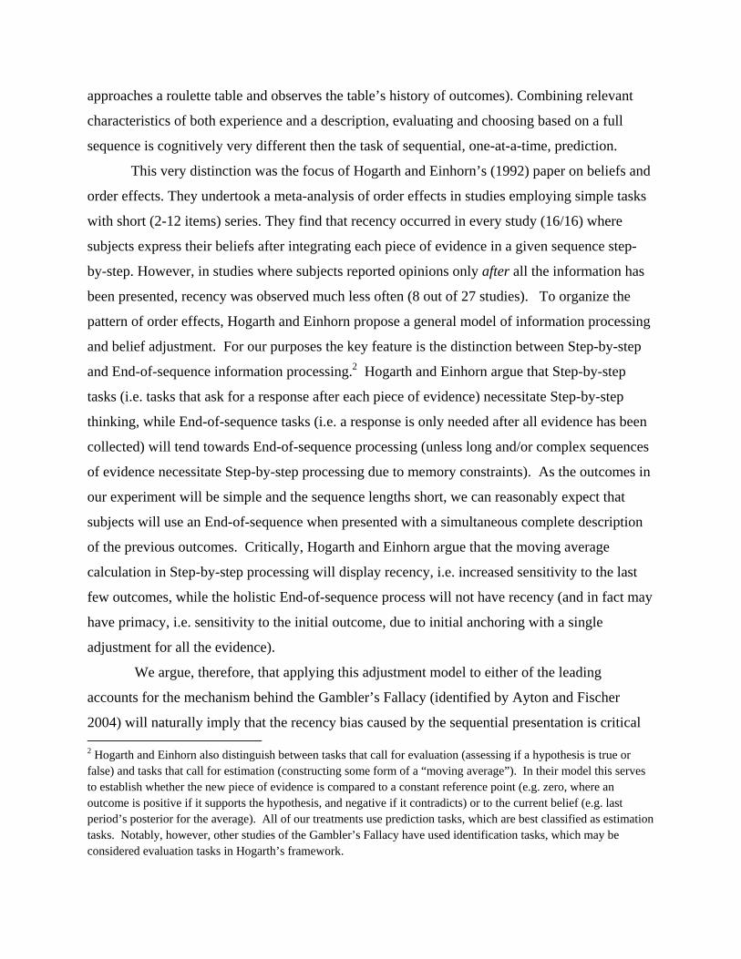
Following Jarvik (1951) and Ayton and Fischer (2004) we calculated the probability,

across subjects, that a prediction continues the color of the previous run for runs of length 1-6.3

Probabilities smaller than 0.5 represent negative recency, the Gambler’s Fallacy. Figure 1

presents the resulting curves for the two conditions. The visual impression supports the paper’s

3 There were too few runs of greater length to do useful analysis.

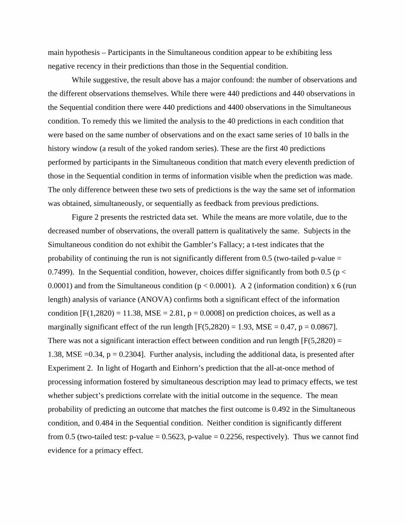
main hypothesis – Participants in the Simultaneous condition appear to be exhibiting less

negative recency in their predictions than those in the Sequential condition.

While suggestive, the result above has a major confound: the number of observations and

the different observations themselves. While there were 440 predictions and 440 observations in

the Sequential condition there were 440 predictions and 4400 observations in the Simultaneous

condition. To remedy this we limited the analysis to the 40 predictions in each condition that

were based on the same number of observations and on the exact same series of 10 balls in the

history window (a result of the yoked random series). These are the first 40 predictions

performed by participants in the Simultaneous condition that match every eleventh prediction of

those in the Sequential condition in terms of information visible when the prediction was made.

The only difference between these two sets of predictions is the way the same set of information

was obtained, simultaneously, or sequentially as feedback from previous predictions.

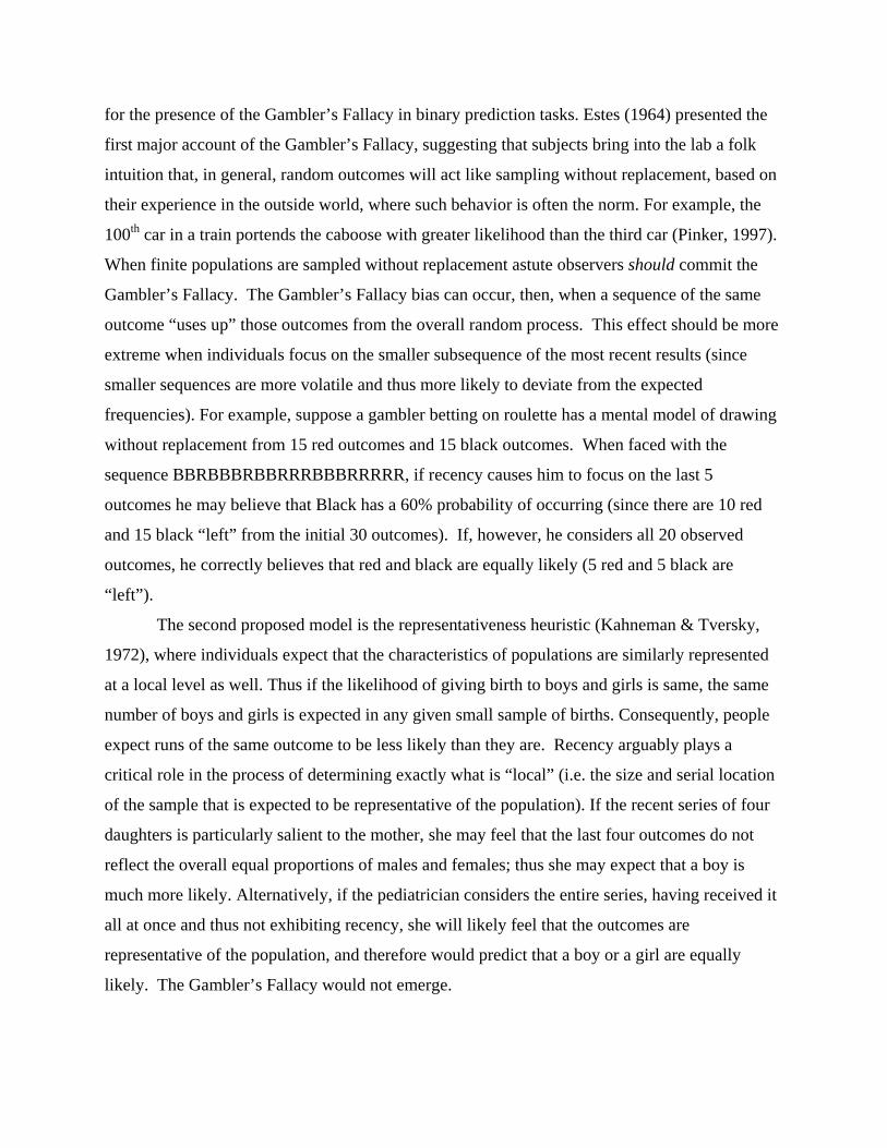
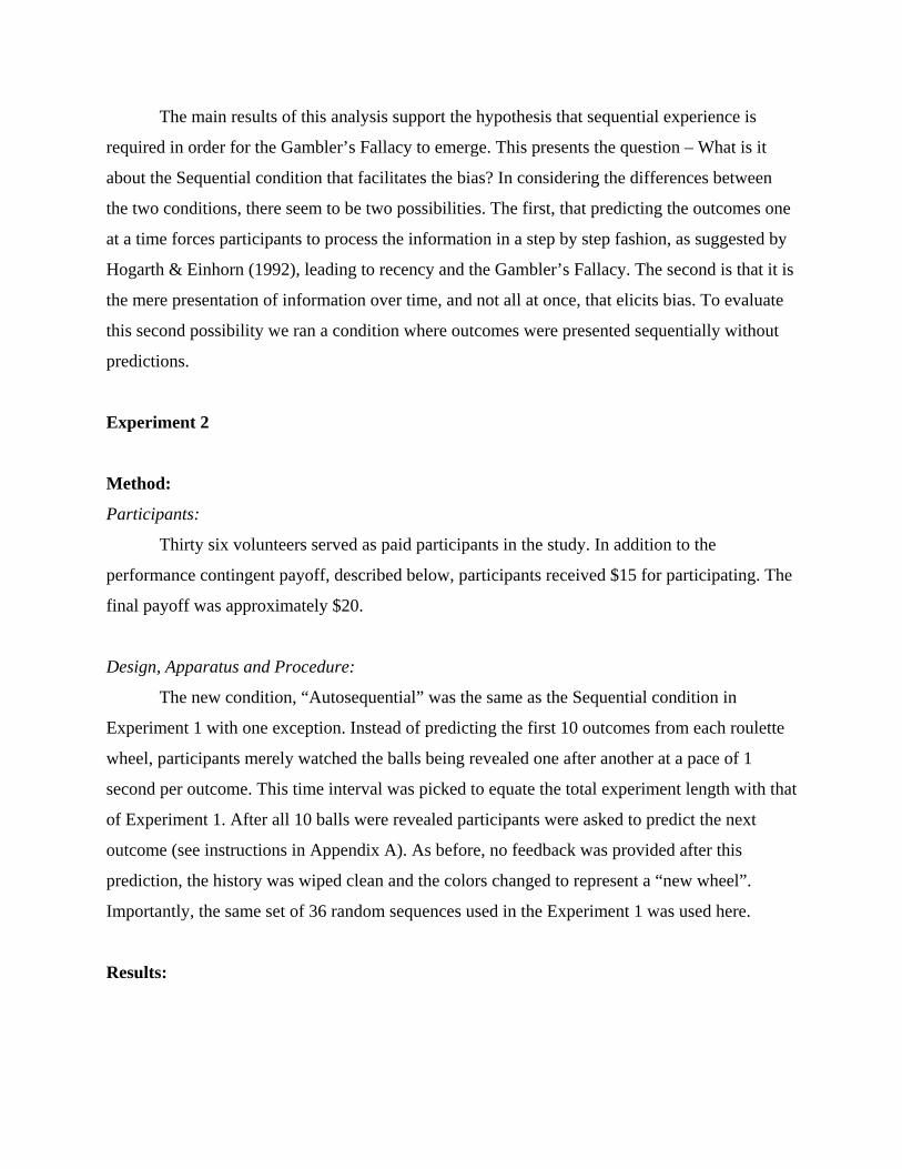
Figure 2 presents the restricted data set. While the means are more volatile, due to the

decreased number of observations, the overall pattern is qualitatively the same. Subjects in the

Simultaneous condition do not exhibit the Gambler’s Fallacy; a t-test indicates that the

probability of continuing the run is not significantly different from 0.5 (two-tailed p-value =

0.7499). In the Sequential condition, however, choices differ significantly from both 0.5 (p <

0.0001) and from the Simultaneous condition (p < 0.0001). A 2 (information condition) x 6 (run

length) analysis of variance (ANOVA) confirms both a significant effect of the information

condition [F(1,2820) = 11.38, MSE = 2.81, p = 0.0008] on prediction choices, as well as a

marginally significant effect of the run length [F(5,2820) = 1.93, MSE = 0.47, p = 0.0867].

There was not a significant interaction effect between condition and run length [F(5,2820) =

1.38, MSE =0.34, p = 0.2304]. Further analysis, including the additional data, is presented after

Experiment 2. In light of Hogarth and Einhorn’s prediction that the all-at-once method of

processing information fostered by simultaneous description may lead to primacy effects, we test

whether subject’s predictions correlate with the initial outcome in the sequence. The mean

probability of predicting an outcome that matches the first outcome is 0.492 in the Simultaneous

condition, and 0.484 in the Sequential condition. Neither condition is significantly different

from 0.5 (two-tailed test: p-value = 0.5623, p-value = 0.2256, respectively). Thus we cannot find

evidence for a primacy effect.

The main results of this analysis support the hypothesis that sequential experience is

required in order for the Gambler’s Fallacy to emerge. This presents the question – What is it

about the Sequential condition that facilitates the bias? In considering the differences between

the two conditions, there seem to be two possibilities. The first, that predicting the outcomes one

at a time forces participants to process the information in a step by step fashion, as suggested by

Hogarth & Einhorn (1992), leading to recency and the Gambler’s Fallacy. The second is that it is

the mere presentation of information over time, and not all at once, that elicits bias. To evaluate

this second possibility we ran a condition where outcomes were presented sequentially without

predictions.

Experiment 2

Method:

Participants:

Thirty six volunteers served as paid participants in the study. In addition to the

performance contingent payoff, described below, participants received $15 for participating. The

final payoff was approximately $20.

Design, Apparatus and Procedure:

The new condition, “Autosequential” was the same as the Sequential condition in

Experiment 1 with one exception. Instead of predicting the first 10 outcomes from each roulette

wheel, participants merely watched the balls being revealed one after another at a pace of 1

second per outcome. This time interval was picked to equate the total experiment length with that

of Experiment 1. After all 10 balls were revealed participants were asked to predict the next

outcome (see instructions in Appendix A). As before, no feedback was provided after this

prediction, the history was wiped clean and the colors changed to represent a “new wheel”.

Importantly, the same set of 36 random sequences used in the Experiment 1 was used here.

Results:

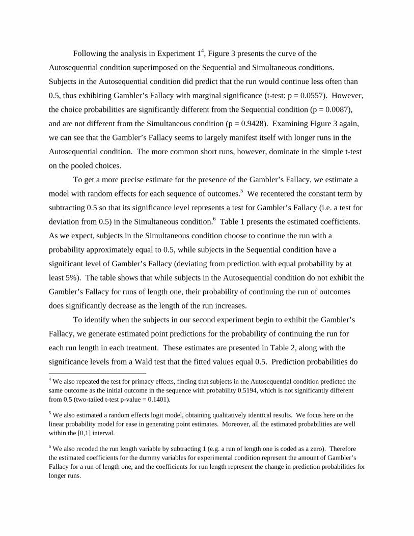
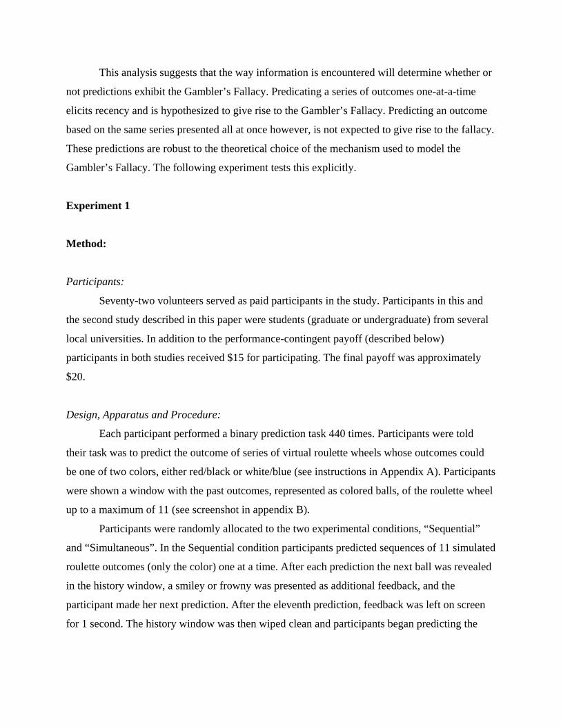
Following the analysis in Experiment 14, Figure 3 presents the curve of the

Autosequential condition superimposed on the Sequential and Simultaneous conditions.

Subjects in the Autosequential condition did predict that the run would continue less often than

0.5, thus exhibiting Gambler’s Fallacy with marginal significance (t-test: p = 0.0557). However,

the choice probabilities are significantly different from the Sequential condition (p = 0.0087),

and are not different from the Simultaneous condition (p = 0.9428). Examining Figure 3 again,

we can see that the Gambler’s Fallacy seems to largely manifest itself with longer runs in the

Autosequential condition. The more common short runs, however, dominate in the simple t-test

on the pooled choices.

To get a more precise estimate for the presence of the Gambler’s Fallacy, we estimate a

model with random effects for each sequence of outcomes.5 We recentered the constant term by

subtracting 0.5 so that its significance level represents a test for Gambler’s Fallacy (i.e. a test for

deviation from 0.5) in the Simultaneous condition.6 Table 1 presents the estimated coefficients.

As we expect, subjects in the Simultaneous condition choose to continue the run with a

probability approximately equal to 0.5, while subjects in the Sequential condition have a

significant level of Gambler’s Fallacy (deviating from prediction with equal probability by at

least 5%). The table shows that while subjects in the Autosequential condition do not exhibit the

Gambler’s Fallacy for runs of length one, their probability of continuing the run of outcomes

does significantly decrease as the length of the run increases.

To identify when the subjects in our second experiment begin to exhibit the Gambler’s

Fallacy, we generate estimated point predictions for the probability of continuing the run for

each run length in each treatment. These estimates are presented in Table 2, along with the

significance levels from a Wald test that the fitted values equal 0.5. Prediction probabilities do 4 We also repeated the test for primacy effects, finding that subjects in the Autosequential condition predicted the same outcome as the initial outcome in the sequence with probability 0.5194, which is not significantly different from 0.5 (two-tailed t-test p-value = 0.1401).

5 We also estimated a random effects logit model, obtaining qualitatively identical results. We focus here on the linear probability model for ease in generating point estimates. Moreover, all the estimated probabilities are well within the [0,1] interval.

6 We also recoded the run length variable by subtracting 1 (e.g. a run of length one is coded as a zero). Therefore the estimated coefficients for the dummy variables for experimental condition represent the amount of Gambler’s Fallacy for a run of length one, and the coefficients for run length represent the change in prediction probabilities for longer runs.

not differ from 0.5 for any run length in the Simultaneous condition, while they differ

significantly for all run lengths in the Sequential condition. In the Autosequential condition,

there is a significant amount of Gambler’s Fallacy for runs of length at least three (and a

marginally significant effect for runs of length 2). Subjects in the Autosequential condition

deviate from choosing each outcome with equal probability by 5.5% for runs of length three, and

deviate by as much as 13.5% for runs of length six (compared to deviations from equal

probability by 9.3% and 15.6% in the Sequential condition). Thus when the Gambler’s Fallacy

does manifest for longer runs, it has a substantial effect (though somewhat smaller than the

Sequential condition). Moreover, while the estimated probabilities for the Autosequential

condition differ significantly from the Sequential condition for runs of length one and two (Wald

test: p = 0.0185 and p = 0.0350, respectively), for longer runs the probabilities do not differ

significantly (run length three to six: p = 0.1306, p = 0.3897, p = 0.6072, p = 0.7535). Thus, it

seems that the Autosequential condition is closer to the Sequential condition than the

Simultaneous condition.

Discussion:

We examine whether experienced information is necessary for the emergence of the Gambler’s

Fallacy in a binary prediction task. In two experiments participants predicted the colored

outcome of a virtual roulette wheel. Information about past outcomes was acquired in one of

three ways 1) experienced sequentially, as the feedback from past predictions 2) simply

presented sequentially one second at a time, or 3) described simultaneously as a set of past

outcomes. The results show that while the Gambler’s Fallacy emerges in the two conditions

where information is experienced sequentially over time, there was no tendency towards

negative recency when past outcomes are encountered as a description (in the form of a

temporally ordered list). Returning to one of the paper’s motivating examples, this suggests that

while an expecting mother with a past birth order of (MMFMMMFFFF) may tend to believe that

a boy is now due, a pediatrician who encounters this information all at once will not exhibit the

same tendency.

This papers main contribution is in delineating a boundary condition for the emergence of

a well known cognitive bias. Our results are broadly consistent with Hogarth and Einhorn’s

(1992) analysis showing that recency emerges robustly when information is revealed step by step

but not when information is acquired all at once. As discussed above, both of the leading

mechanisms for the Gambler’s Fallacy (Estie 1962, Kahnemann & Tversky 1972) imply recency

as a contributing factor to the bias. However, the results of our second experiment suggest that

merely presenting the information sequentially may be sufficient to cause recency effects, even if

choices are not required until the end of the sequence. In contrast, Hogarth and Einhorn assume

that, if the outcomes are simple and the sequence is short, a task that asks for a choice at the end

of the sequence of outcomes will activate a process that does not exhibit recency. Therefore, our

results can serve to enrich their model by suggesting a more complete set of criteria to determine

when a Step-by-step process (exhibiting recency) or an End-of-sequence process (without

recency) will be activated. Additionally, we fail to find evidence for a primacy effect in the

Simultaneous condition, as predicted by Hogarth and Einhorn’s model.

A second account for our results can be derived from an elaboration to Oskarsson, et.

al.’s (2008) theoretical work on random and non-random binary sequences and hidden Markov

processes. That paper argues that individuals form a mental model of the outcome-generating

process that is a Markov process. They argue that the described characteristics of the process

(such as whether it is “subjectively random”, whether the nonrandom cause is intentional or not,

how much control the non-random cause has, and whether the non-random causes’ goals are

simple or complex) lead individuals to assume different features about the mental Markov

process. Depending on the described characteristics, individuals may construct Markov models

where the outcomes will be independent over time, or follow trends. They may also conceive of

models that shift between states or cycle through states. While their model does not explicitly

differentiate within the “subjectively random” category based on the means by which

information is provided (they argue that this category as a whole should elicit the Gambler’s

Fallacy), their framework is general enough that one could imagine augmenting their model in

that direction. Possibly, presenting information sequentially draws more attention to the

alternating nature of the series. This may lead to a mental model of a process with a greater

emphasis on negative recency (as opposed to independence) and to predictions consistent with

this belief. While the first account assumes that experience leads people to overweight recent

information, the second assumes that experience leads to exaggerated beliefs about the

alternating nature of the sequence. Further work is needed to examine the accounts’ relative

contributions to the current results.

The current results also contribute to the effort to more sharply define experience. In

doing so we seek the minimal set of stimulus characteristics that elicit significantly different

behavior then that observed when information is described. We found that passive experience,

the observing of outcomes revealed over time, was both necessary and sufficient for the

Gambler’s Fallacy to emerge. Interestingly, Hertwig, et. al. (2004) similarly found that the

passive sampling of outcomes, without incurring gain or loss, was sufficient in order to observe

behavior, such as the underweighting of rare events, which is consistent with past studies of

decisions from experience. Taken together, these results suggest that qualitatively different

processes are engaged when people merely encounter information sequentially over time. Since

this is the way we encounter information in so many contexts (financial personal, professional,

etc.), future research should continue to revisit “classic” BDT phenomena using experience-

based paradigms. The current results continue to suggest this is a potentially valuable endeavor.

Identifying additional contexts where behavior differs from decisions from description will

extend the existing literature, and our efforts here, to identify and map the important boundaries

between the phenomena of description-based and experience-based decisions.

The conclusions of the current study are necessarily limited to the Gambler’s Fallacy in

predicted binary sequences. As noted in the introduction, the Gambler’s Fallacy is also observed

in generation tasks, where participants are asked to generate a series that looks random, and

identification tasks, where series are classified as random or not. Prediction is unique in that

generation and identification tasks alert the participant as to the topic of the study (Ayton &

Fischer, 2004). Quite possibly, the task of identifying a series as random is an evaluation task (in

the sense of Hogarth & Einhorn, 1992), which is hypothesized not to exhibit recency, rather than

an estimation task. If so, we would not expect to find an effect of information presentation in an

identification task.

Future work that examines the effect of presentation (simultaneous/descriptive vs.

sequential/experiential) and of paradigm (prediction, generation and identification) on behavior

is needed (see McDonald & Newell, 2008, for one recent example). One suggestive result is that

positive recency (i.e. the hot hand) was observed both in a prediction task with sequential

information (NBA free throws) and in an indentification task with simultaneously described

outcomes (Gilovich, Vallone & Tversky, 1985).This result is more suggestive than conclusive as

it confounds presentation and paradigm (and examines positive recency). However, together with

the present study it serves to motivate further study of experience’s role in the cognitive biases.

References:Ayton, P. & Fisher, I. (2004). The Gambler’s Fallacy and the Hot-Handed Fallacy: two Faces of Subjective Randomness. Memory & Cognition. 32, 1369-1378.

Bar-Hillel, M. & Wagenaar, W. A. (1991). The Perception of Randomness. Advances in Applied Mathematics, 12, 428-454.

Barron, G., & Erev, I. (2003). Feedback-based decisions and their limited correspondence to description-based decisions. Journal of Behavioral Decision Making, 16, 215-233.

Barron, G., Ursino, G., & Yechiam, E. (2008). Underweighting Rare Events in Experience-based Decisions: Beyond Sample Error. Harvard Business School Working Paper, No. 08-077.

Budescu, D. V. (1987). A Markov Model for Generation of random Binary Sequences. Journal of Experimental Psychology, 13, 25-39.

Erev, I., & Barron G. (2005). On adaptation, maximization, and reinforcement learning among cognitive strategies. Psychological Review, 112, 912-931.

Estes, W. K. (1964). Probability learning. In A.W. Melton (Ed.), Categories of human learning, 88-128. New York: Academic Press.

Fox, C. R. & Hadar, L. (2006). Decisions from experience = sampling error + prospect theory: Reconsidering Hertwig, Barron, Weber & Erev (2004). Judgment and Decision Making, 1, 159-161.

Gilovich, T., Vallone, R., & Tversky, A. (1985). The hot hand in basketball: On the misperception of random sequences. Cognitive Psychology. 17(3). 295-314.

Hertwig, R., Barron, G., Elke, W., & Erev, I. (2004). Decisions from experience and the effect of rare events in risky choices. Psychological Science, 15, 534-539.

Hogarth, R. M. & Einhorn, H. J. (1992). Order Effects in Belief Updating: The belief-Adjustment Model. Cognitive Psychology, 24, 1-55.

Jarvik, M. E. (1951). Probability learning and a negative recency effect in the serial anticipation of alternative symbols. Journal of Experimental Psychology, 41, 291-291.

Kahneman, D., & Tversky, A. (1979). Prospect theory: An analysis of decision under risk. Econometrica, 47, 263-291.

Kahneman, D. & Tversky, A. (1972). Subjective probability: A judgment of representativeness. Cognitive Psychology, 3, 430-454.

Lee, W. (1971). Decision theory and Human Behavior. New York: John Wiley & Sons, Inc.

Laplace, P. S. (1951). A Philosophical Essay on Probabilities. (Translated by F.W. Truscott and F.L. Emory). New York: Dover.

McDonald, F., & Newell, B. (2008). Effects of alternation rate and prior belief on the interpretation of binary sequences. University of New South Wales Working Paper.

Newell, B. R. & Rakow, T. (2007). The role of experience in decisions from description. Psychonomic Bulletin & Review, 14, 1133-1139.

Oskarsson, A. Van Boven, L., McClelland, G., & Hastie, R. (2008). What’s next? Judging Sequences of Binary Events. University of Colorado Working Paper.

Pinker, S. (1997). How the Mind Works. New York: Norton.

Tversky, A., & Kahneman, D. (1992). Advances in prospect theory: cumulative representation of uncertainty. Journal of Risk and Uncertainty, 9, 195-230.

Weber, E. U., Blais, A. R., & Shafir, S. (2004). Predicting risk sensitivity in humans and lower animals: Risk as variance or coefficient of variation. Psychological Review, 111, 430-445.

Figure 1.

Probability of continuing previous run as a function of run length across subjects in Simultaneous and Sequential conditions.

Figure 2.

Probability of continuing previous run as a function of run length across subjects in Simultaneous and Sequential conditions – 40 yoked trials.

0

0.1

0.2

0.3

0.4

0.5

0.6

1 2 3 4 5 6

Simultaneous Sequential 

0

0.1

0.2

0.3

0.4

0.5

0.6

1 2 3 4 5 6

Simultaneous Sequential 

Prob.

Run Length

Run Length

Prob.

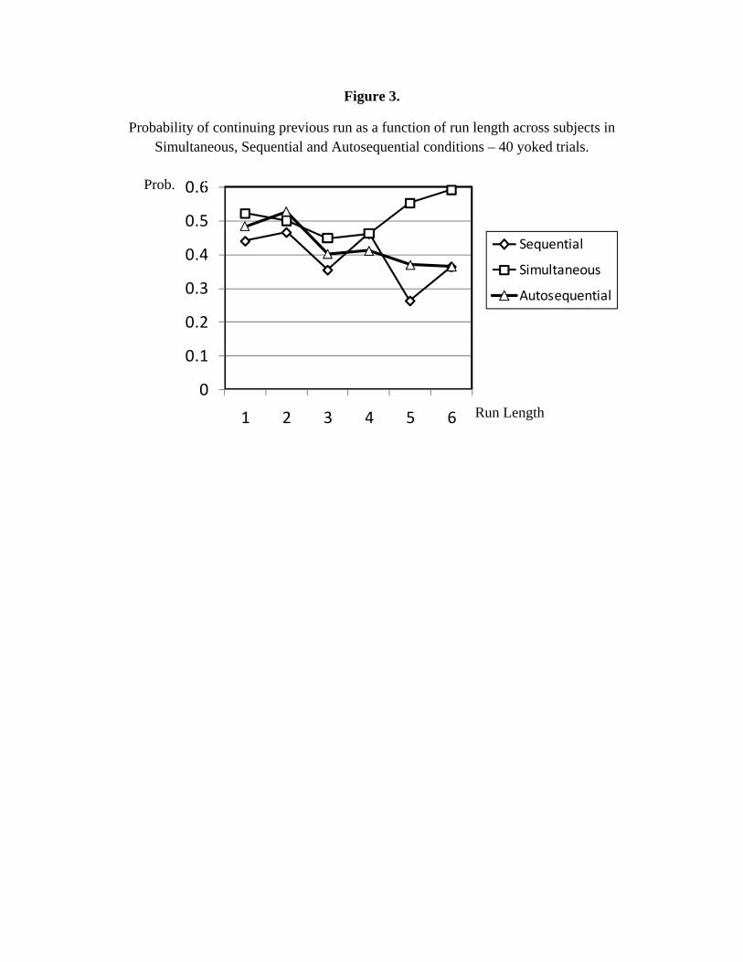
Figure 3.

Probability of continuing previous run as a function of run length across subjects in Simultaneous, Sequential and Autosequential conditions – 40 yoked trials.

0

0.1

0.2

0.3

0.4

0.5

0.6

1 2 3 4 5 6

Sequential 

Simultaneous 

Autosequential

Run Length

Prob.

Table 1

Pr[Choice Continues the Run] β  Robust 

Std. Err. 

Dummy for Sequential  ‐0.0624*** 0.023Dummy for Autosequential  ‐0.0129 0.023Run Length (for Sequential)  ‐0.0209* 0.011Run Length (for Simultaneous)  ‐0.00769 0.011Run Length (for Autosequential)  ‐0.0266** 0.011Constant [Simultaneous baseline]  0.0110 0.019  Observations  4248Number of series  36

GLS regression with random effects by outcome series Constant term recentered by subtracting 0.5*** p<0.01, ** p<0.05, * p<0.1 

Table 2

Estimated Probability of Continuing the Run

Condition Run Length

1  2 3 4 5  6

Simultaneous  0.511  0.503  0.496  0.488  0.480  0.473    (0.019)  (0.16) (0.20) (0.029) (0.039)  (0.050)

Sequential  0.449***  0.428*** 0.407*** 0.386***  0.365*** 0.344***

   (0.019)  (0.016) (0.020) (0.0.28) (0.038)  (0.048)

Autosequential  0.498  0.471* 0.445*** 0.418***  0.392*** 0.365***

   (0.019)  (0.016) (0.020) (0.028) (0.038)  (0.048)

Robust Standard Errors in parenthesesWald test that fitted probability = 0.5: *** p<0.01, ** p<0.05, * p<0.1

Appendix A

Participants instructions for the three experimental conditions in Experiments 1 and 2..

Welcome,

In this game your goal is to predict the outcomes of a series of roulette wheels with different pairs of colors.

[SEQUENTIAL: In each round you may choose one of the two colored buttons on the screen. The computer will then randomly generate an outcome that will be one of the two colors. Like a real roulette wheel, the chances for each color being the outcome are equal. A “History” window will display the last 10 outcomes of the game. After every 11 outcomes the game will change over to the next roulette wheel.]

[SIMULTANIOUS: For each round the computer will randomly generate 10 consecutive outcomes that will be displayed from left to right in the “History” window. Like a real roulette wheel, the chances for each color being the outcome are equal. Your task is to then predict the next outcome by choosing one of the two colored buttons on the screen. The outcome will then be randomly generated by the computer. For the next round, the computer will generate 10 new outcomes from the next roulette wheel.]

[AUTOSEQUENTIAL: For each trial, the computer will randomly generate the first 10 outcomes that will be displayed in the “History” window. Like a real roulette wheel, the chance of each of the two colors being the outcome is equal. Your task is to then predict the next outcome by choosing one of the two colored buttons that will appear on the screen. That outcome will then be randomly generated by the computer. The computer will then generate 10 outcomes from the next roulette wheel and again you will make a prediction.]

This process is repeated for a predetermined number of rounds until the experiment is over.

At the end of the experiment, your earnings will depend on only two of the previous rounds, randomly selected by the computer. For each of the two rounds you will receive $5 if you correctly predicted the outcome of that round. Aside from the two rounds, you will also receive $15 for participating.

As in all CLER experiments, deception is not used and all the information above is both true and accurate.

Appendix B

Four screenshots from the experiment.

Top screen: A prediction is elicited. Participant chose “Blue”, which was correct (second from top). A new set of ten outcomes then appears (third from top). Participant predicts “Red”, which was incorrect (bottom screen).