Embed Size (px)
Citation preview

Making the Finite Difference Time Domain computational method better... stronger...
faster (at a cost much much less than $6M)
Rodolfo E. DíazMichael Watts
Igor Scherbatko
Laboratory for Material Wave Interactions

Standard FDTD on the Yee grid is based on a Cartesian finite difference version of
Maxwell’s Curl Equations
• The Yee lattice intercalates E and H in space, making the definitions of the curl operators straight-forward.
The Yee unit cell:
At the (i,j,k) point E is on the edges, H is on the faces.
x y
z
Hx Hy
Hz
Ez
Ex Ey
z
x y

The Fields are advanced in time by considering the Curl term to be the source over the timestep.Consider the x component of the Curl of H
x y
z
Hx Ez(j)
Ey(k+1)
Ez(j+1)
Ey(k)
yzx
x
Ez
Ey
Et
B
dz
kjiEkjiE
dy
kjiEkjiE
t
B yyzz
x
,,1,,,,,1,

Similarly, the x component of the Curl of H drives Dx
-Hy(k)
-Hz(j-1)
Ex
z
x y
Hy(k-1)
Hz(j)
yzx
x
Hz
Hy
Ht
D
dz
kjiHkjiH
dy
kjiHkjiH
t
D yyzz
x
1,,,,,1,,,

This is an Initial Value PDE problem that can be solved from time = t to
t+dt
To solve the inhomogeneous PDE in discretized time, set up a leapfrog scheme:
If H is evaluated at the half-integer steps while E is evaluated at the integer steps, the curl acts as a source term.
time
t t+dt t+dt/2
E(t+dt)
E(t)
Assume H (and therefore curl H) is constant at the value it had at t+dt/2 ,throughout the timestep
H

We therefore have a PDE with constant coefficients and a constant inhomogeneous term.
•We have two alternatives:
Solve the initial value problem:
So that
(gives an exponential characteristic solution)
HEt
dtt Rt
Rwith
Ht
E
1

Or turn the equation into finite difference form :
The time derivative of E is clearly evaluated at the half-integer step.
So is the curl of H.
Therefore so must be E(?)=(E(t+dt)+E(t))/2
2/11
1
1
1
1
n
r
nn Hdt
dtdt
dtEE
r
e
r
e
r
e
2
1
2
1
2
1
Now, call Now, call t+dt tt+dt t
2
dtt
t
E
time
t t+dt t+dt/2
E(t+dt)
E(t)
E(t+dt/2)
2
dttH
2
1?
dttHE
dt
tEdttE
rr
e

The simulation proceeds from E to H, from H to E, satisfying BCs
automatically
• What’s the problem?• Because all of space must be discretized we
have a problem with the computational volume. • Small details (fine grid) or Large objects
translate into Large Scenes• Large scenes =
– Large Memory requirement – Long Time of execution

What are the assets of FDTD?
• Full wave time domain solution lets you see the physics of the problem.
• Simple to program = Intuitive• Eminently Stable.• No theoretical limit on ability to solve a
problem (no matrix inversion).• Trade-off of CPU memory versus time.

The domain must be truncated in such a way that…
• The scatterer is nevertheless illuminated with the correct incident field.– Plane wave injection.
• The scattered energy exits the domain as if it were in an infinite space.– Absorbing Boundary Conditions (ABCs)
• The scattered energy is available for observation with minimized interference by the (blinding) incident wave.– Separation of Total field and Scattered field
regions

Our Goal is to improve the performance of FDTD with the
simplest possible fixes
• Performance: •Greater accuracy for same domain size•Faster execution for same domain size•Same accuracy for minimized domain size
•Simplicity:•Of derivation, implementation and execution•Low computational overhead

Today’s Presentation
•Field Teleportation: Injection of True Plane Waves into Finite domains.
•Allows separation of total field and scattered field regions.•With no apriori analytical solution of the environment.
•Field Teleportation of arbitrary time domain fields

Today’s Presentation (continued)
•Symmetrized FDTD•Removes Yee asymmetry from material discontinuities.•Reduces “staircasing”error.
•A new Radiation Boundary Condition •Simple to program•Beats the PML

Why do we need Plane wave injection?
•(Near) Plane Wave illumination is a fact of life in many applications:
•RCS, Remote Ground Penetrating Radar schemes, Laser inspection of semiconductor surfaces... Almost all optical scattering problems.
•In these, the background scattering is uniform (enough) and not of interest, we want to measure the response of the isolated defect.

•To maximize SNR we don’t want our ABCs to have to deal with the strong incident plane wave.
•Previous authors have tried to generate these “local” plane wave regions with analytic Huygens sources.
In the most challenging cases, the incident wave is >> the
scatter
ABC
Huygens Sources
Scattered Field Region Total
Field Region

•That is, without causing scattering from the FDTD grid which is itself an anisotropic dispersive object.•What if there is no analytic solution?
The Huygens sources must create and absorb a large number of waves
transparently.
ABC
Huygens Sources
Scattered Field Region
Total Field Region

•FDTD is not a discrete-time/discrete-space approximation of Maxwell’s equations. It is a discrete time simulation of the behavior of a medium where every element is only connected to its nearest neighbors, and obeys the same Hamiltonian as Maxwell’s Equations.
•G. F. Fitzgerald built a tabletop example of this medium in the late 1880’s.
The Answer: Use FDTD to create the Huygen’s sources.
Pulleys
Rubber bands
H=spinD=strain

In this discrete space, Schelkunoff’s currents have exact discrete analogs
•And they are trivial to implement:
Etotal
Htotal
Sources Etotal
Htotal
E=0
H=0Ke=n x Htotal
Km=-n x Etotal
Sources
dsKHEt
Jt
DH ee /
dsHnt
E totexcess /ˆ1
dsHndt
E totalRR
eexcess /ˆ
2
11
1

Hz(i,j)
Ex(i,j+1)
Ey(i,j)
Ex(i,j)
Ey(i+1,j)
-
+
-
E H
H E
-
-
Problem domain window
Source domain window
(a) (b)
+
+
+
Similarly for Hexcess; so that the fields inside a “Window”can be teleported
from one domain to another

Since Plane waves are infinite, they cannot be created in a
finite domain
•However, they can be created in a periodic domain...
•And copied onto another domain

Demo: Scattering from a cylinder
Run FDTD302a.EXE (after compiling it)It should be inserted into this presentation as a hyperlink
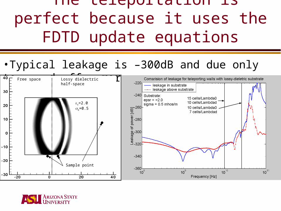
The teleportation is perfect because it uses the FDTD
update equations
•Typical leakage is –300dB and due only to round-off error Lossy dielectric half-space
Free space
r=2.0e=0.5
Sample point
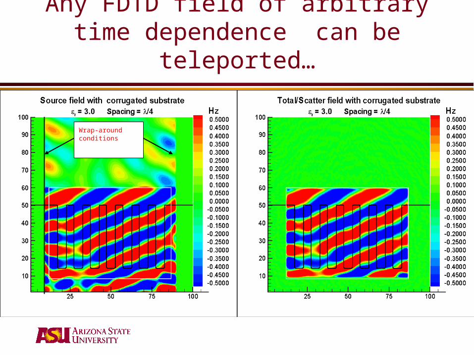
Any FDTD field of arbitrary time dependence can be
teleported…
Wrap-around conditions

To determine how a defect in a complex environment alters the signature of the
environment

Next subject:Yee’s grid assures us second
order accuracy but it is asymmetric
(i,j,k)
(i,j,k-1)
Ez Hx
Ey
mat2z
mat1z
Mat1y Mat2y
(i,j,k+1)
• This is inconvenient when modeling material objects – where is the real boundary?
•But even worse, how do you model a smooth surface?
•Staircasing is supposed to be a major source of “noise”in Cartesian FDTD.

The partially filled capacitor is equivalent to an effective
medium
kjikji
kjikji
x kji
,,1,,
,,1,,2,,
2
1
,,
,,
,,,,
,,
,,
,,
,,
1,,
21
21
21
n
kjix
kji
kjixnkji
kjix
kji
kjix
kji
nkji H
t
t
xEt
t
xE
Standard FDTD update equation
Exi,j,k
Media #1i,j,kMedia #2i+1,j,k
• Series sum of two caps
• Only applies to up and right
• This undos the asymmetry of the Yee grid

Symmetrizing removes the asymmetry error from the staircasing approximation
• Ordinary FDTD • Symmetrized FDTD
Run SymP1.EXE (after compiling it)It should be inserted into this page as a hyperlink
Run SymP2.EXE (after compiling it)It should be inserted into this page as a hyperlink

This can improve dramatically the range of validity of coarse (fast)
models
• Ordinary and Symmetrized FDTD compared to the exact solution for Cylinder RCS

So far…
•We can inject perfect plane waves into finite domains.
•Separates the Scattered Field from the Total field for maximum SNR•Illuminates finite objects with true model of typical incident wave.
•We can create smooth material objects without having to reduce the grid size.
•Speeds up execution

The Next step:Minimize the domain size
•This is the job of the Absorbing Boundary Condition.
•These are traditionally derived by taking analytic solutions to one-sided wave equations (Mur) or ideal fictitious absorbing materials (PML) and discretizing into FDTD.
•But that was precisely the problem with Huygen’s sources…

So instead use Self-Teleportation
•The Radiation Boundary Condition:
Recipe:
•Teleport the exiting field back into the source space with a minus sign.
•Repeat as needed
•Terminate with a simple one-cell absorber
Ex(i,jlow)
Hz(i,jlow)
Ex(i,jlow+1)
Hz(i,jlow-1)
- -
Figure 6. Teleportation of fields with a negative sign to the cell below the lower radiation boundary creates a subtracting wave.

Scheme of the 2D FDTD experiment (field termination in free space and dielectric
media )
300 400 500 600 700300
400
500
600
Dielectric = 2
Z
Y
300 400 500 600 700300
400
500
600
Dielectric = 2
Z
Y
P – polarized, harmonic cylindrical wave (Hx component)
PEC
field measurement plane PEC 12 cells ABC

Comparison new ABC and Berenger’s PML*
12-cellsABC
0 15 30 45 60 75 90-100
-80
-60
-40
-20
0
Free space ( = 1 )
circles -> = 12 s
squares -> = 18 s
triangles -> = 24 s
stars -> = 30 s
Berenger's 10 -cells PML
Ref
lect
ion,
dB
Angle of incidence, deg.
•Data is taken from
W.Yu, R. Mittra, et al.
“FDTD modeling of an
artificially synthesized absorbing medium”, IEEE Microwave and Guided Wave Lett.,
Vol. 9, N0.12, Dec.1999.

Y
Z
400 450 500 550 600
475
500
525
550
575
600
Lossy dielectric Free space
6 - cells ABC 1 - cell Huygen' s termination
Source
A more challenging problem:Field termination on the lossy dielectric/free
space interface

The Radiation boundary Condition is impervious to material discontinuities
-80 -60 -40 -20 0 20 40 60 80
-100
-80
-60
-40
-20Free spaceLossy dielectric
Ref
lect
ion,
dB
Angle of incidence, deg.
6 - cellsABC
o:r=4-j0.6, :r=4-j0.75, : r=4-j1.0

An even more challenging problem: How does this
Radiation Boundary Condition fare with Surface Waves?
Incident Wave
Curvature scatter Trailing edge
wrap-around and scatter
•The TM Radar Cross section of an airfoil is a surface wave dominated phenomenon.
Creeping Wave
Traveling Wave

Compare a large domain to one with the RBC at 3 cells from the creeping
wave
•The large domain •The small domain
Run SurfP1.EXE (after compiling it)It should be inserted into this page as a hyperlink
Run SurfP2.EXE (after compiling it)It should be inserted into this page as a hyperlink

The time domain history of the echoes differs only
slightly
• The RBC dampens the source so compare in Freq. Domain
0 35 70 105 140 175 210 245 280 315 3500.06
0.048
0.036
0.024
0.012
0
0.012
0.024
0.036
0.048
0.060.06
0.06
Echosmalli
Echolargei
3500 iTimestep
Hz

The spectral content of the incident pulses show the effect of
the RBC
• Input > -50dB below 3 cells/ point
0 50 100 150100
90
80
70
60
50
40
30
20
10
00
100
5020 log freqSLi
20 log freqSSi
1750
115
i
Large
Small
ds=/3
Grid cut-off
Frequency

The frequency domain echoes are extremely close to each other
0 50 100 15040
30
20
10
0
10
20
30
4024.368
37.522
20 log ratioLi
20 log ratioSi
1750
115
i
ds=/3
Grid cut-off
Frequency

0 50 100 1505
4
3
2
1
0
1
2
3
4
55
5
1
1
dBdiffi
1750
115
i
Up to 0.66 fcutoff the typical deviation is less than 1dB
ds=/3
Grid cut-off
ds=/4
Frequency
Note: In this region the RBC starts <<1 from the object

Conclusions
•We can inject perfect plane waves (or any field for that matter) into finite domains.
•We can create smooth material objects without having to reduce the grid size.
•We can truncate the FDTD domain extremely close to the scattering object (< 1) regardless of the complexity of the environment in which that object is submerged.

FDTD…Better, Stronger,
Faster…
All at less than $6M