“Making Sense of Inter-Signal Corrections: Accounting for

July/August 2009

Inside GNSS July/August 2009 Appendix Page 1 of 18

“Making Sense of Inter-Signal Corrections: Accounting for GPS Satellite Calibration Parameters in Legacy and Modernized Ionosphere Correction,” — Appendices

Avram Tetewsky Charles Stark Draper Laboratory Jeffry Ross The MITRE Corporation Arnold Soltz, Norman Vaughn, Jan Anszperger, Chris O’Brien, Dave Graham, Doug Craig, and Jeff Lozow Charles Stark Draper Laboratory

Graham, Doug Craig, and Jeff Lozow Charles Stark Draper Laboratory

Appendix A: Relevant Sections of IS-GPS-200 Appendix A: Relevant Sections of IS-GPS-200 Throughout the main article, sections of IS‐GPS‐200 are quoted. In this appendix, relevant sections of IS‐GPS‐200 have been collected together in one place for easy reference and are presented here. Throughout the main article, sections of IS‐GPS‐200 are quoted. In this appendix, relevant sections of IS‐GPS‐200 have been collected together in one place for easy reference and are presented here.

Modernized dual frequency correction algorithm valid for all ranging codes but with L2C and L1 C/A used as examples. Assumes dual‐frequency compensation.

20.3.3.3.3.3 Ionospheric Correction. The two frequency (L1 P(Y) and L2 P(Y)) user shall correct for the group delay due to ionospheric effects by applying the relationship:

2 1

1L PY L PYPR PRPR γ

γ−

=−

Where

• PR = pseudorange corrected for ionospheric effects,

• PRLi,x = pseudorange measured on the channel indicated by the subscript

and γ is as defined in paragraph 20.3.3.3.3.2. The clock correction coefficients are based on "two frequency" measurements and therefore account for the effects of mean differential delay in SV instrumentation.

Table A-1: Modernized and legacy ionosphere free pseudorange equations

30.3.3.3.1.1.2 L1 /L2 Ionospheric Correction. The two frequency (L1 C/A and L2 C) user shall correct for the group delay and ionospheric effects by applying the relationship:

2 12 1 / 2 12 1 /

12

( )1

L C L C A L C L C AGD

PR PR c ISC ISCPR cTγ γγ

− + −= −

−

where, • PR = pseudorange corrected for

ionospheric effects, • PRLi,x = pseudorange measured on the

channel indicated by the subscript, (we changed “i” to “Li,x”)

• ISCLi,x = inter-signal correction for the channel indicated by the subscript (see paragraph 30.3.3.3.1.1),

• TGD = see paragraph 20.3.3.3.3.2, • c = speed of light,

and where, denoting the nominal center frequencies of L1 and L2 as fL1 and fL2

respectively, ( ) ( )2 22

12 L1 L2(f / f ) 1575.42 /1227.6 77 / 60γ = = = .

Legacy dual‐frequency correction algorithm valid only for PY ranging codes or works if single‐frequency compensation

July/August 2009


Table A-2: IS-GPS-200 ISC and delay definition pages, along with the additional single-frequency compensation

20.3.3.3.3.2 L1 - L2 Correction. The L1 and L2 correction term, TGD, is initially calculated by the CS to account for the effect of SV group delay differential between L1 P(Y) and L2 P(Y) based on measurements made by the SV contractor during SV manufacture. The value of TGD for each SV may be subsequently updated to reflect the actual on-orbit group delay differential. This correction term is only for the benefit of "single-frequency" (L1 P(Y) or L2 P(Y)) users; it is neces-sitated by the fact that the SV clock offset estimates reflected in the af0 clock correction coefficient (see paragraph 20.3.3.3.3.1) are based on the effective PRN code phase as apparent with two frequency (L1 P(Y) and L2 P(Y)) iono-spheric corrections. Thus, the user who utilizes the L1 P(Y) signal only shall modify the code phase offset in accordance with paragraph 20.3.3.3.3.1 with the equation (ΔtSV)L1P(Y) = ΔtSV - TGD

where TGD is provided to the user as subframe 1 data. For the user who utilizes L2 P(Y) only, the code phase modification is given by (ΔtSV)L2P(Y) = ΔtSV - γTGD where, denoting the nominal center frequencies of L1 and L2 as fL1 and fL2 respectively, γ = (fL1/fL2)2 = (1575.42/1227.6)2 = (77/60)2. The value of TGD is not equal to the mean SV group delay differential, but is a measured value that represents the mean group delay differential multiplied by 1/(1- γ). That is, TGD =(tL1P(Y) - tL2P(Y))/ 1 - γ where tLiP(Y) is the GPS time the ith frequency P(Y) signal (a specific epoch of the signal) is transmitted from the SV antenna phase center.

3.3.1.7 Equipment Group Delay. Equipment group delay is defined as the delay between the signal radiated output of a specific SV (measured at the antenna phase center) and the output of that SV's on-board frequency source; the delay consists of a bias term and an uncertainty. The bias term is of no concern to the US since it is included in the clock correction parameters relayed in the NAV data, and is therefore accounted for by the user computations of system time (reference paragraphs 20.3.3.3.3.1, 30.3.3.2.3). The uncertainty (variation) of this delay as well as the group delay differential between the signals of L1 and L2 are defined in the following. 3.3.1.7.1 Group Delay Uncertainty. The effective uncertainty of the group delay shall not exceed 3.0 nanoseconds (two sigma). 3.3.1.7.2 Group Delay Differential. The group delay differential between the radiated L1 and L2 signals (i.e. L1P(Y) and L2 P(Y), L1 P(Y) and L2 C) is specified as consisting of random plus bias components. The mean differential is defined as the bias component and will be either positive or negative. For a given navigation payload redundancy configuration, the absolute value of the mean differential delay shall not exceed 15.0 nanoseconds. The random variations about the mean shall not exceed 3.0 nanoseconds (two sigma). Corrections for the bias components of the group delay differential are provided to the US in the Nav message using parameters designated as TGD (reference paragraph 20.3.3.3.3.2) and Inter-Signal Correction (ISC) (reference paragraph 30.3.3.3.1.1). 3.3.1.8 Signal Coherence. All transmitted signals for a particular SV shall be coherently derived from the same on-board frequency standard; all digital signals shall be clocked in coincidence with the PRN transitions for the Psignal

30.3.3.3.1.1.1 Inter-Signal Group Delay Differential Correction. The correction terms, TGD, ISCL1C/A and ISCL2C, are initially provided by the CS to account for the effect of SV group delay differential between L1 P(Y) and L2 P(Y), L1 P(Y) and L1 C/A, and between L1 P(Y) and L2 C, respectively, based on measurements made by the SV contractor during SV manufacture. The values of TGD and ISCs for each SV may be subsequently updated to reflect the actual on-orbit group delay differential. For maximum accuracy, the single frequency L1 C/A user must use the correction terms to make further modifications to the code phase offset in paragraph 20.3.3.3.3.1 with the equation: (ΔtSV)L1C/A = ΔtSV - TGD + ISCL1C/A

where TGD (see paragraph 20.3.3.3.3.2) and ISCL1C/A are provided to the user as Message Type 30 data, described in paragraph 30.3.3.3.1.1. For the single frequency L2 C user, the code phase offset modification is given by: (ΔtSV)L2C = ΔtSV - TGD + ISCL2C

where, ISCL2C is provided to the user as Message Type 30 data. The values of ISCL1C/A and ISCL2C are measured values that represent the mean SV group delay differential between the L1 P(Y)-code and the L1 C/A- or L2 C-codes respectively as follows, ISCL1C/A = tL1P(Y) - tL1C/A

ISCL2C = tL1P(Y) - tL2C. where, tLix is the GPS time the ith frequency x signal (a specific epoch of the signal) is transmitted from the SV antenna phase center

20.3.3.3.3.1 User Algorithm for SV Clock Correction. The polynomial defined in the following allows the user to determine the effective SV PRN code phase offset referenced to the phase center of the antennas (Δtsv) with respect to GPS system time (t) at the time of data transmission. The coefficients transmitted in subframe 1 describe the offset apparent to the two-frequency user for the interval of time in which the parameters are transmitted. This estimated correction accounts for the deterministic SV clock error characteristics of bias, drift and aging, as well as for the SV implementation characteristics of group delay bias and mean differential group delay. Since these coefficients do not include corrections for relativistic effects, the user's equipment must determine the requisite relativistic correction. Accordingly, the offset given below includes a term to perform this function. The user shall correct the time received from the SV with the equation (in seconds) t = tsv - Δtsv (1) where

• t = GPS system time (seconds), • tsv = effective SV PRN code phase time at message

transmission time (seconds), • Δtsv = SV PRN code phase time offset (seconds).

The SV PRN code phase offset is given by Δtsv = af0 + af1(t - toc) + af2(t – ttoc)2 + Δtr (2)

July/August 2009

July/August 2009 Appendix Page 3 of 18

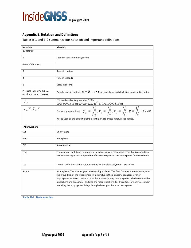
Appendix B: Notation and Definitions Tables B‐1 and B‐2 summarize our notation and important definitions.

Notation Meaning

Constants

C Speed of light in meters /second

General Variables

R Range in meters

t Time in seconds

τ Delay in seconds

R c tρ = + •PR (used in IS‐GPS‐200), ρ (used in most text books)

Pseudorange in meters, , a range term and clock bias expressed in meters

ith L band carrier frequency for GPS in Hz, L1=154*10.23 106 Hz, L2=120*10.23 106 Hz, L5=115*10.23 106 HzLif

12, 15, 25,γ γ γ γ

12, 15 25

2 2 21 1 2

2 2 22 5 5

, , ,L L L

L L L

21

22

L

L

f f f ff f f

γ γ γ γ= = = =

Frequency squared ratio, f

; L1 and L2

will be used as the default example in this article unless otherwise specified.

Abbreviations

LOS Line of sight

Iono Ionosphere

SV Space Vehicle

Trop Troposphere, for L‐band frequencies, introduces an excess ranging error that is proportional to elevation angle, but independent of carrier frequency. See Atmosphere for more details.

Toc Time of clock, the validity reference time for the clock polynomial expansion

Atmos Atmosphere: The layer of gases surrounding a planet. The Earth's atmosphere consists, from the ground up, of the troposphere (which includes the planetary boundary layer or peplosphere as lowest layer), stratosphere, mesosphere, thermosphere (which contains the ionosphere and exosphere) and also the magnetosphere. For this article, we only care about modeling the propagation delays through the troposphere and ionosphere.

Table B-1: Basic notation

Inside GNSS 4 of 18

Definition Symbol, Term, or

Expression

Modernized GPS satellites have different signals (or modulations/ranging codes) for different classes of users. Civilians can access C/A, L2C, and L5I/L5Q signals. Military users have the P(Y) and M signals. On the L1 carrier frequency, ‘x’ represents either the C/A, P(Y), or M code signals on that carrier. On the L2 carrier frequency, ‘z’ represents either the L2C, P(Y), or M code signals on that carrier or if using the L5 carrier, ‘z’ represents the L5I/L5Q Note that IS‐GPS‐200 generically uses “Li,x” as a generic placeholder. Because the satellite electronics can’t be delay free, or perfectly identical for all signal paths, all of these signals emerge from the “antenna phase center” at slightly different times and from different spatial L band antenna phase/delay centers.

Signals/modulations/ ranging codes Li,x or Li,z xth signal on Li= L1 carrier; zth signal on Li=L2 or L5 carrier

,Li xt Defined in IS‐GPS‐200 30.3.3.3.1.1.1., this is the GPS time tag associated with a specific chip coming from the SV.

We will show that it is the same as the hardware delay in the SV such that at a common observation time, one

identifies which chip emerges from the SV.

The additional SV equipment delay in seconds (3.3.1.7) on the xth signal on the Li’th carrier frequency, due to the

signal having to travel through different electrical paths, and emerging from distinctly located antenna

phase/group delay centers. There is an electrical delay, and a spatial delay (antenna phase/group delay center)

delay. See Appendix G,” Phase and Group Delay Centers for Antennas.”

,Li xτ

The inter‐signal correction, defined in IS‐GPS‐200 30.3.3.3.1.1.1, in terms of either the GPS time tag difference or hardware delay defined above as:

,Li xISC

, these parameters apply only to the modernized IIR‐M and IIF satellites. To be precise, we show in section 3.1 that this equality holds.

Legacy scaled group delay differential parameters defined to be

GDT, see 20.3.3.3.2 IS‐GPS‐200.

2Li

Af

Ionosphere, for L band frequencies, introduces an excess ranging error in meters that is inversely proportional to

L band carrier frequency squared,_iono LiR

2Li

Af

; , where A = 40.3 times the total electron content along the line of sight

path through the ionosphere. There are higher order terms.

tropR Troposphere, for L band frequencies, introduces an excess ranging error that is proportional to elevation angle, but independent of L band carrier frequency

Ionosphere free pseudorange

2, 1,

1L z L xρ γ ρ

γ− •−

Defined in IS‐GPS‐200, 20.3.3.3.3.3, yields a pseudorange without an ionosphere term for

P(Y) codes, where 2,L zρ 1,L xρis the pseudorange measured with z’th signal on the L2 carrier, and is the

pseudorange measured with the x’th signal on the L1 carrier.

July/August 2009


1, 2,

1L x L zρ ρ

γ−−

Ionosphere difference algorithm

, an algorithm that is less noisy, discussed in popular GPS textbooks, that differences out common

terms that may have higher dynamics than the remaining terms. (See the publications by Kaplan, E., and C. Hegarty, and Misra, P. and P. Enge, cited in the Additional Resources section of the main article.)

2, 1,

1L PY L PY

YIFDCTτ γ τ

γ− •

=−

The delay due to the YIFDC, Y code Ionosphere Free Delay Center; the effective departure point for the

ionosphere free pseudorange combination measurement using L1 PY and L2PY code. If L1PY and L2PY happen to

depart from the same point, then, this expression also yields that point.

GPSt True GPS time, a perfect time scale that resets at the beginning of each week to 0.

The effective SV timing error on each signal emerging from the satellite, it includes a common oscillator error

(first term), modeled by a broadcast 2nd order polynomial valid for typically 2 hours, and the signal specific delay

previously defined in this table (2nd term)

_ ,

_ _ , sv Li x

clock in SV Li x

t

t

δ

τ

=

−

The coefficients are: af0, the clock offset in seconds, the af1 term is the linear drift rate in seconds per second, and the af2 term, the quadratic clock error in seconds per seconds squared.

u gps biast t t= + A model of time in the user’s GPS receiver, perfect GPS time corrupted by a time varying bias. By taking 4 or

more pseudorange measurements, the user solves for the time varying bias.

Table B-2: Fundamental definitions

July/August 2009


Appendix C: Geometry used in “The Precise Positioning Error Budget” Figure C‐1 is reprinted from the U.S. Air Force, “The Precise Positioning Service (PPS) Performance Standard,” <http://gps.afspc.af.mil/gpsoc/documents/PPS_PS_Signed_Final_23_Feb_07.pdf>

Segment Error Source

UERE Contribution (95%) w/o WAGE(meters)

Zero AOD

Max. AODin

Operation14.5 Day

AOD

Space

Clock StabilityGroup Delay StabilityDif’l Group Delay StabilitySatellite Acceleration UncertaintyOther Space Segment Errors

0.00.00.00.01.0

8.90.62.02.01.0

2570.62.02041.0

Control

Clock/Ephemeris EstimationClock/Ephemeris PredictionClock/Ephemeris Curve FitIono Delay Model TermsGroup Delay Time CorrectionOther Control Segment Errors

2.00.00.8N/AN/A1.0

2.06.70.8N/AN/A1.0

2.02061.2N/AN/A1.0

User

Ionosheric Delay CompensationTropospheric Delay compensationReceiver Noise and ResolutionMultipathOther User Segment Errors

4.53.92.92.41.0

4.53.92.92.41.0

4.53.92.92.41.0

95% System UERE (PPS) 7.5 13.8 388*for illustration only, actual PPS receiver performance varies significantly – see Table B.2-1

AOD = age of dataThe other space errors are probably due to the SV antenna

Table A.4-1. Dual-Frequency P(Y)-Code UERE Budget Without WAGE.

H

Projection = +H x sin(13.88o)

Projection = 0

Projection = -H x sin(13.88o)

13.88o

13.88o

Not to scale

Figure A.4-6. Illustration of Spatial Dependency – Horizontal Orbit Error

Terrestrial Service Volume

Alt = 3000 km

41.3o

Not to scaleFigure A.3-2. Illustration of Terrestrial Service Volume.

Figure C-1: Geometry approximations for surface users and for navigation in the greater terrestrial sphere

http://gps.afspc.af.mil/gpsoc/documents/PPS_PS_Signed_Final_23_Feb_07.pdf

Inside GNSS 7 of 18

Appendix D: Mathematical Identity The derivation of equation (11) from the main text is shown here:

Inside GNSS

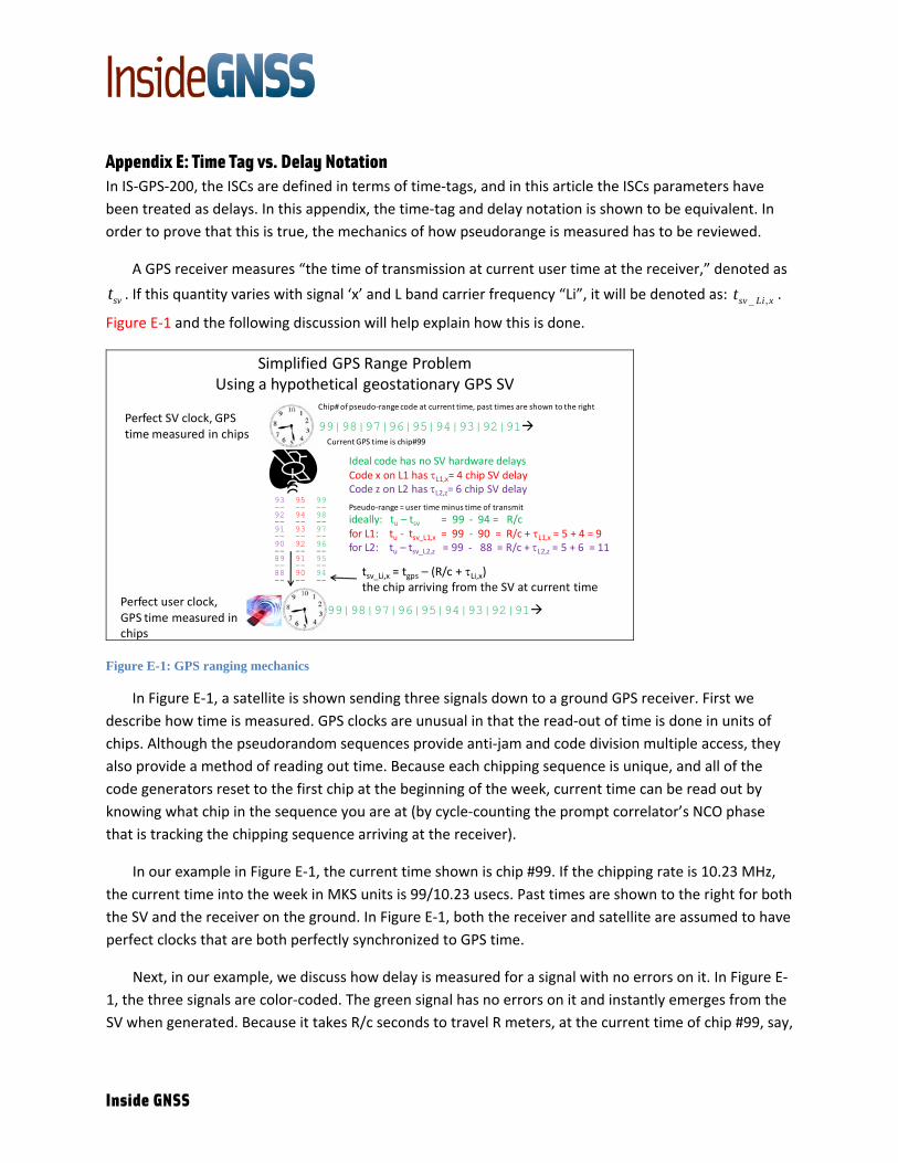
Appendix E: Time Tag vs. Delay Notation In IS‐GPS‐200, the ISCs are defined in terms of time‐tags, and in this article the ISCs parameters have been treated as delays. In this appendix, the time‐tag and delay notation is shown to be equivalent. In order to prove that this is true, the mechanics of how pseudorange is measured has to be reviewed.

A GPS receiver measures “the time of transmission at current user time at the receiver,” denoted as

svt _ ,sv Li xt. If this quantity varies with signal ‘x’ and L band carrier frequency “Li”, it will be denoted as: .

Figure E‐1 and the following discussion will help explain how this is done.

Simplified GPS Range ProblemUsing a hypothetical geostationary GPS SV

99|98|97|96|95|94|93|92|91Perfect SV clock, GPS time measured in chips

Ideal code has no SV hardware delaysCode x on L1 has τL1,x= 4 chip SV delayCode z on L2 has τL2,z= 6 chip SV delay

Perfect user clock, GPS time measured in chi s

99|98|97|96|95|94|93|92|91

93 99-- --92 98-- --91 97-- --90 96-- --89 95-- --88 94-- -- --

95--94--93--92--91--90

Chip# of pseudo‐range code at current time, past times are shown to the right

Pseudo‐range = user time minus time of transmit

ideally: tu – tsv = 99 ‐ 94 = R/c

for L2: tu – tsv_L2,z = 99 ‐ 88 = R/c + τL2,z = 5 + 6 = 11

Current GPS time is chip#99

tsv_Li,x = tgps – (R/c + τLi,x)the chip arriving from the SV at current time

for L1: tu ‐ tsv_L1,x = 99 ‐ 90 = R/c + τL1,x = 5 + 4 = 9

p

Figure E-1: GPS ranging mechanics

In Figure E‐1, a satellite is shown sending three signals down to a ground GPS receiver. First we describe how time is measured. GPS clocks are unusual in that the read‐out of time is done in units of chips. Although the pseudorandom sequences provide anti‐jam and code division multiple access, they also provide a method of reading out time. Because each chipping sequence is unique, and all of the code generators reset to the first chip at the beginning of the week, current time can be read out by knowing what chip in the sequence you are at (by cycle‐counting the prompt correlator’s NCO phase that is tracking the chipping sequence arriving at the receiver).

In our example in Figure E‐1, the current time shown is chip #99. If the chipping rate is 10.23 MHz, the current time into the week in MKS units is 99/10.23 usecs. Past times are shown to the right for both the SV and the receiver on the ground. In Figure E‐1, both the receiver and satellite are assumed to have perfect clocks that are both perfectly synchronized to GPS time.

Next, in our example, we discuss how delay is measured for a signal with no errors on it. In Figure E‐1, the three signals are color‐coded. The green signal has no errors on it and instantly emerges from the SV when generated. Because it takes R/c seconds to travel R meters, at the current time of chip #99, say,

Inside GNSS

svtchip #94 is just arriving at the receiver. Thus, , the time of transmission as measured at current user

time at the receiver would be chip #94.

The receiver measures this time directly because the tracking loop is aligning the replica code with the incoming code. With the replica code aligned with the incoming signal, the prompt correlator tap

NCO code phase can be read out and the receiver measures svt , the time of transmission as seen at the

receiver at current time, to be chip #94 when current time is chip #99 as counted out from the receiver’s

reference clock. Differencing the time of transmission, svt , of chip #94 from current time, chip #99, one

measures the transmit time as being five chips (99‐94). Thus, the range is five chips.

Given that we know that each chip is 1/chiprate seconds long — in this case, 10.23 MHz, we have measured the range by knowing which chip number we are at in the pseudorandom spreading

sequence. In general, for any time t, using the GPS time base, svt is analytically modeled

as sv GPSRt tc

= − , assuming there are no other errors. Other errors such as the ionosphere and

troposphere can easily be included in this term, adding them to the range term.

Current received time, as measured in the receiver, with a perfect clock synchronized to GPS

would also be . Thus, the uncompensated measured range, ,

receivert

GPStLi x

, as a function of receiver time

minus time of transmission as measured at current receiver time with perfect equipment would be:

umR

,

_ _ , _

_

_ , _

(E.1)

t t a receiver with a perfect GPS clock

= transmit time, or time it left the SV at c

Li xumreceiver noerr sv Li x noerr

receiver noerr GPS

sv Li x noerr

Rt t

c

t

= −

=

__ , _

urrent receiver time

= t t LOS trop iono Lisv Li x noerr GPS

R R Rc

+ += −

Performing the indicated math yields for perfect user and perfect SV clock case:

_ _ , _

2

2

t

= [ ( )]

= (E.2)

Li

Li

umreceiver noerr sv Li x noerr

LOS tropLi

gps gps

um LOS tropLi

Rt

cAR Rft t

cAR R Rf

= −

+ +− −

+ +

Next, as shown in Figure E‐1, the x’th signal code generator can have a signal and an L‐band carrier–

unique offset: ,Li xτ . Suppose the L1P(Y) code is delayed an additional amount, 1,L PYτ chips (shown in red

July/August 2009


with a value of 1,L PYτ of four chips), and the L2P(Y) code is delayed by 2,L PYτ chips shown in purple (with

a value of six). The indicated range in both cases is increased by four and six chips, respectively, because it takes longer to come out, and the chip arriving at the receiver has an earlier time tag on it. Hence, the difference from current time increases as range increases when these terms are positive. This

establishes the sign convention that will be used for ,Li xτ , that these delays increase measured

pseudorange.

We need to digress for a moment and comment about our use of the symbol ,Li xτ a delay, versus

,Li xt defined in IS‐GPS‐200 30.3.3.3.1.1.1, as a GPS time tag. In the end, they both yield the same

numerical answers, both characterize the delays within the hardware, and both can be used to

quantitatively define the ISC values as differences between delays Lτ ,i x or differences between time‐

tags ,Li xt .

In Figure E‐1, if you asked “At what GPS time do you see chip #92?”, you have to wait an extra four chip periods for the red L1P(Y) code, an extra 6 chip periods for the L2P(Y) purple code to find that particular chip than a path with no delays (green); if you were R meters way, you would have to wait out

an additional delay of R/c. Thus, the GPS time‐tag tL ,i x defined in IS‐GPS‐200 30.3.3.3.1.1.1 as a function

of hardware delay ,Lτ i x is:

, , + E.2a)Li x gps Li xRt tc

τ= + (

Instead, if you asked the question we asked: “At some instant in time, which chips do you see at a particular range as a function of the code you are looking at?”, then, you are asking for time of transmission of:

_ , ,( + ) (Esv Li x gps Li xRt tc

τ= − .2b)

Each expression has its use, but given that:

• we will be working with GPS receivers that will be measuring all of the time of transmissions at the same collection time instant, and

• we need to build a model of the satellite, and also, because we use delay lines, we need delay parameter place holders,

therefore, working with our delay model and delay parameters, ,Li xτ is more useful than working with a

time‐tag model for finding a common chip value.

July/August 2009


,

Given that the ISC values are differences of (E.2a), the delay values fit in exactly as the time‐tag values would. Using (E.2a) and the definition of the ISC, we see that

, 1, , 1,Li x L PY Li x L PY Li xISC t t τ τ= − = − . Although this is a bit pedantic, we could not risk using a symbol

already used by IS‐GPS‐200 to mean something different.

Appendix F: IS-GPS-200 Notation Road Map

In IS‐GPS‐200, Figure 20‐3 (shown here with annotations as Figure F‐1), is an extremely insightful diagram about how the GPS correction parameters inter‐relate to each other with respect to an overall model of how the pseudorange is formed, measured, and corrected; thus, it serves as an excellent road map for summarizing how the modernized parameters fit together with the legacy parameters.

Figure F‐1: Using IS‐GPS‐200 Figure 20‐3 as a road map for the modernized parameters

1. In Figure F‐1, the original Figure 20‐3 shows true GPS time (tgps), as generated by a perfect clock, being corrupted by “code phase offsets” that originate in the satellite. This corruption is shown by adding errors to GPS time (tgps) in the middle left of Figure F‐1. The original list consisted of

the true SV clock effects, differential group delay errors (τLi,x), and relativistic effects. In our article, we formally assigned the variable dtsv_Li,x to represent all of the satellite errors that are being added to true GPS time, which can be functions of the specific code ‘x’ on the i’th L band, Li. Using the IS‐GPS‐200 list for the first 3 terms, we have:

Inside GNSS

a. the common clock modeled by the af0, af1, and af2 polynomial

b. the signal unique delays, τLi,x, using a negative sign so that these additional delays add to the range,

c. relativitistic corrections, although we don’t bother to track these in detail in this discussion

d. We also want to include the special compensation that is applied to the SV to make the L1PY and L2PY equipment delays transparent to the dual frequency L1PY and L2PY user. In the equipment group delay differential signal errors, this is done by subtracting the

term 2

11L PY L PYτ γτ

γ−−

from each delay, leaving the TGD‐ISCLi,x term as the remaining error.

Thus the total SV equipment error term becomes:

_ , _ _ ,

2 1_ _ ,

_ _ ,

t =t -( -T ))

=t -( - )1

=t

sv Li x clock in SV Li x YIFDC

L PY L PYclock in SV Li x

clock in SV GD Li xT ISC

δ τ

τ γττγ

−−

− +

and 2

_ _ 1 2( ) ( ) ; is the validity timeclock in SV fo f toc f toc toct a a t t a t t t= + − + −

2. In section 2 of Figure F‐1, IS‐GPS‐200 lists the standard propagation model used in most text books: the line of sight range, ionosphere, and troposphere, contributing a total delay of.

_LOS iono Li tropR R Rc

+ +seconds.

3. Section 3 of figure F‐1 shows how true GPS time, corrupted by satellite equipment errors, followed by a propagation model, becomes a modernized time of transmission model of the current chip being received at current time of:

__ , _ , LOS iono Li trop

sv Li x gps sv Li x

R R Rt t t

cδ

+ +⎛ ⎞= + − ⎜ ⎟

⎝ ⎠

Using items 1‐3, we now have a complete model of SV. Up until now, not one text book or article in the literature had a hardware model of the SV’s delay with af0 adjustment because, up until now, there were no new signals. However, with the modernized IIR‐M and IIF satellites, a compelling need has emerged for this model because not all users will want to work with the ionosphere‐free pseudorange algorithm due to its noise amplification properties. Without a generic model of the SV and the time of transmission model, users cannot derive alternative modernized ionosphere algorithms and correctly account for the hardware equipment errors.


biast

4. Section 4 of Figure F‐1 summarizes the model of the GPS receiver’s time as a user receiver time bias being added to true gps time:

= u GPSt t +

5. Section 5 of figure F‐1 shows the pseudorange error model that include the new terms and the effects of the built in L1PY/L2PY compensation. By executing the definition of pseudorange as user time minus time of transmission as measured at current receiver time, the result for the un‐compensated pseudorange is:

,

,

__ , _ ,

_ _ _

[ ( )] = t

= c t ( )

Li x

Li x

um LOS trop iono Liu sv Li x bias sv Li x

um bias LOS trop iono Li clock in SV GD Li x

R R Rt t t

c cR R R c t T ISC ,

ρδ

ρ

+ += − + −

• + + + − • − +

Section 5 is a bit tricky to notate because a feedback loop is being closed showing how these uncompensated pseudoranges are also being compensated/removed.

6. In section 6 of Figure F‐1, we have summarized the new compensation algorithms. The current IS‐GPS‐200 document breaks the compensation down into a series of special cases based on whether a dual or single frequency correction is being made, and whether it is for legacy or modernized signals. This is summarized below:

July/August 2009


Raw time of transmission _ ,sv Li xt is measured from the prompt NCO code phase,

__ , _ ,

21 2 ,

( ) (3.1.16)

= ( [ ( ) ( ) - ( )])

LOS trop iono Lisv Li x GPS sv Li x

LOS troGPS f toc f toc GD Li x

R R Rt t t

cR R

t a t t a t t T ISC

δ+ +

= + −

++ − + − − −

,

_

2_ 1 2 ,

OR ( ) [( ( ) ( ) )] + ( ) (3.1.15)

Li x

p iono Li

um bias LOS trop iono Li f toc f toc GD Li x

Rc

c t R R R c a t t a t t c T ISCρ

+

= + + + − • − + − • −

svtΔ_ ,sv Li xtCompensate using a per 20.3.3.3.3.1 that just removes the common

clock term with broadcast 0 1, ,

As shown in the main article, all of these cases can be handled by performing the modernized single frequency compensation of removing c∙(TGD‐ISCLi,x) on each pseudorange, and then using idealized equations on the final pseudoranges.

2f fafa a coefficients which leaves:

, _ 20.3.3.3.3.1

__ , _ 20.3.3.3.3.1 ,

_ ,

= ( [- ( )])

OR ( ) + ( )

Li x

LOS trop iono Lisv Li x sv GPS GD Li x

m bias LOS trop iono Li GD Li x

R R Rt t t T ISC

c

c t R R R c T ISCρ

+ +− Δ + − −

= + + + • −

Generic Single Frequency compensation based

on 20.3.3.3.3.1 0 1 2, ,

Above specializes for PY

Perform Dual Frequency PY code section 20.3.3.3.3

20.3.3.3.3.1_ 2 20.3.3.3.3.1_ 1

1L PY L Pρ γρ

ργ

−=

−

f f fa a a broadcast

polynomial compensation followed by 30.3.3.3.1.1.1 compensation

removing ,( )GD Li xT ISC− term, specializes to

20.3.3.3.3.2 for PY code values

, _ 20.3.3.3.3.1_ _ 30.3.3.3.1.1.1

__ , _ 20.3.3.3.3.1 _30.3.3.3.1.1.1

_

( - )= ( )

OR ( )

Li x and

LOS trop iono Lisv Li x sv sv GPS

m bias LOS trop iono Li

R R Rt t t t

c

c t R R Rρ

+ +− Δ Δ −

= + + +

Perform Dual Frequency algorithm 30.3.3.3.3.1.1.2, valid for all codes,

20.3.3.3.3.1_ 2, 12 20.3.3.3.3.1_ 1, 2, 12 1,

12

( )1

L z L x L z L xGD

c ISC ISCcT

ρ γ ρ γρ

γ− + −

= −−

after this step, the remaining pseudorange is:

, _ 20.3.3.3.3.1_ 30.3.3.3.3.1.1.2 ( )

Li xm bias LOS trc t R Rρ = + +Note: 30.3.3.3.3.1.1.2 becomes 20.3.3.3.3 if you put in PY code values

Above specializes for PY to removing 20.3.3.3.3.2

1,

2,

( ) for L1PY and( ) for L2PY

GD L PY GD

GD L PY GD

T ISC TT ISC Tγ

− =

− =

July/August 2009


Appendix G: Phase and Group Delay Centers for Antennas The publications by Murphy, T., et alia and by Van Graas, F., et alia cited in the Additional Resources in the main article, discuss the recent interest in refining the concept of a “group delay center of an antenna.” Although beyond the scope of this article, a brief discussion of phase, group delay, antenna phase centers, and antenna group delay centers will be given here.

The purpose of the transmit antenna is to couple energy from a transmitter to free space via an impedance transformation to match the output of the transmitter to free space. From a circuit point of view, an antenna can be viewed as a complex load (radiation resistance and load impedance), and as a filter with a potentially different frequency response for each departure angle.

Note that many GPS antenna elements are relatively wide bandpass filters with respect to any one given GPS L band. However, the element pattern can have different responses at each different L band. In addition, when there is an array of elements to create a sharper beam pattern, the array factor that shapes the beam can impart even larger gain, phase, and group‐delay variations between each band; and within any one band, the array factor potentially introduces variations across the beam. Thus, just like a filter, an antenna can have a gain pattern, phase pattern, and although not normally calculated, a group delay pattern that varies with departure angle.

The publications by Kaplan, E., and C. Hegarty, and Misra, P. and P. Enge, cited in Additional Resources, discuss how to understand the concept of group delay, the phase slope with respect to frequency for bandpass signals. For any bandpass signal that is reasonably well behaved over the bandpass region, one can think of there being a unique group‐delay effect on the modulation and a different carrier‐phase effect for the center frequency. If you accept the fact that the antenna has gain, phase, and group delay response that vary with departure angle, you can then work on understanding the concept of a phase center, and then extend that concept to a group delay center.

The phase center is the approximate location from which the carrier frequency appears to emanate from. For some simple antennas, you can analytically factor the magnitude and phase response of the E fields and analytically identify this point. In other cases, a numerical fit is done over a limited set of departure angles. Because the antenna current distributions vary with frequency, there is generally a unique phase center for each L‐band frequency.

Inside GNSS 16 of 18

di

θ

y

z

r

θ

Far field, and also roll angle symmetry assumed in these examples

rms deviation over θ minimized at particular z identifies approximate phase center

volume error curves vs. geometry (ray path) are more useful to end user

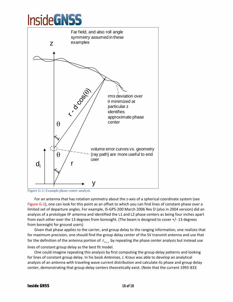
Figure G-1: Example phase center analysis

For an antenna that has rotation symmetry about the z‐axis of a spherical coordinate system (see Figure G‐1), one can look for this point as an offset to which you can find lines of constant phase over a limited set of departure angles. For example, IS‐GPS‐200 March 2006 Rev D (also in 2004 version) did an analysis of a prototype IIF antenna and identified the L1 and L2 phase centers as being four inches apart from each other over the 13 degrees from boresight. (The beam is designed to cover +/‐ 13 degrees from boresight for ground users)

Given that phase applies to the carrier, and group delay to the ranging information, one realizes that for maximum precision, one should find the group delay center of the SV transmit antenna and use that for the definition of the antenna portion of ,Li xτ by repeating the phase center analysis but instead use

lines of constant group delay as the best fit model. One could imagine repeating this analysis by first computing the group delay patterns and looking

for lines of constant group delay. In his book Antennas, J. Kraus was able to develop an analytical analysis of an antenna with traveling wave current distribution and calculate its phase and group delay center, demonstrating that group delay centers theoretically exist. (Note that the current 1993 IEEE

July/August 2009


Antenna Standard only discusses gain and phase center, because up until recently the group delay data had not been needed for most of the applications covered by the IEEE. However, as noted earlier, the GNSS community does recognize the need for group delay analysis of GPS antennas, as noted in Kraus's book and IS‐GPS‐705. )

Finite length wire with traveling wave current at speed p·c, precursor to helix

)]cos(1(2

)([))]}cos(1(

2sin[

)cos(1)sin({

2

θωω

θ θωθ

θπ

ppcb

crtj

o eppcb

prpIZE

−−−

−−

=

))cos(

2(2

))cos(1(2

)(c

brt

pcbp

pcb

crtphase

θωωθωω

−−+−=−−−=

For this antenna, the phase and group delay centers are at the same point because phase is linear in frequency

Suggests bandpass expansions, then spatial expansion around [r - di cos(θ)] functions for fitting center data.

Figure G-2: Analytical example taken from Kraus showing phase and delay centers

Note that in the example taken from Kraus (Figure G‐2), the antenna current distribution was

assumed to be independent of frequency; hence his idealized result shows a phase and group delay center that is independent of frequency. In reality, many GPS antennas that consist of a single element have an antenna pattern that is a wideband bandpass model; each GPS L band has a different gain, phase, and delay response. However, when you have an antenna made up of an array of elements, the spatial locations of the elements, and the weights, it effectively creates a finite impulse response filter that can provide additional gain, phase, and group delay variations, which are probably more significant than the element variations due to the current distribution being a function of frequency. For a well‐designed array, the gain, phase, and group delay response can be relatively constant within the beam, but it can vary as one approach the beam edges.

Although IS‐GPS‐200 defines the delay parameters for the ISCs to the point where the signal emanate from the antenna phase center, because ranging codes imply group delay effects, we believe that the ISCs, which are delay parameters, should be measured to the point where the signal emanates from the antenna’s group delay center. The antenna phase center data should be used to build a model of delta pseudorange.

July/August 2009


L1L2 L5

Phase Center Distance from c.g., uncertainty bounds, and position independent phase offsets

φ1

φ2

φ5

Assuming linear delay in ith bandL2 L5

Delay Center Distance from c.g., uncertainty bounds, and position independent delay offsets

τ1τ2τ5

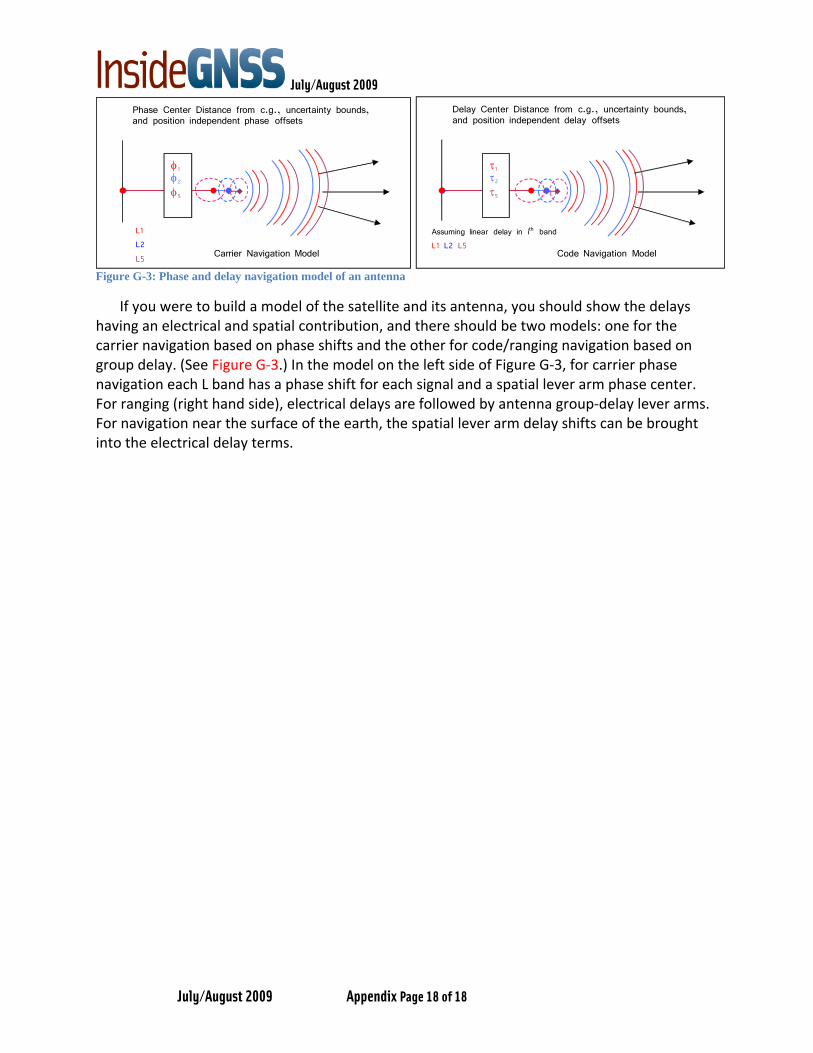
L1 Carrier Navigation Model Code Navigation Model

Figure G-3: Phase and delay navigation model of an antenna

If you were to build a model of the satellite and its antenna, you should show the delays having an electrical and spatial contribution, and there should be two models: one for the carrier navigation based on phase shifts and the other for code/ranging navigation based on group delay. (See Figure G‐3.) In the model on the left side of Figure G‐3, for carrier phase navigation each L band has a phase shift for each signal and a spatial lever arm phase center. For ranging (right hand side), electrical delays are followed by antenna group‐delay lever arms. For navigation near the surface of the earth, the spatial lever arm delay shifts can be brought into the electrical delay terms.

Documents

“Making Sense of Inter-Signal Corrections: Accounting for