Making fractional polynomial models more robust

Willi SauerbreiInstitut of Medical Biometry and Informatics University Medical Center Freiburg, Germany

Patrick RoystonMRC Clinical Trials Unit, London, UK

2

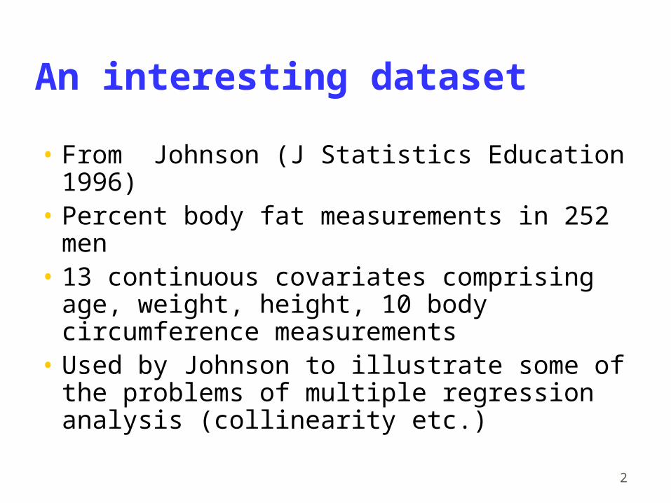
An interesting dataset

• From Johnson (J Statistics Education 1996)• Percent body fat measurements in 252 men• 13 continuous covariates comprising age,

weight, height, 10 body circumference measurements

• Used by Johnson to illustrate some of the problems of multiple regression analysis (collinearity etc.)

3

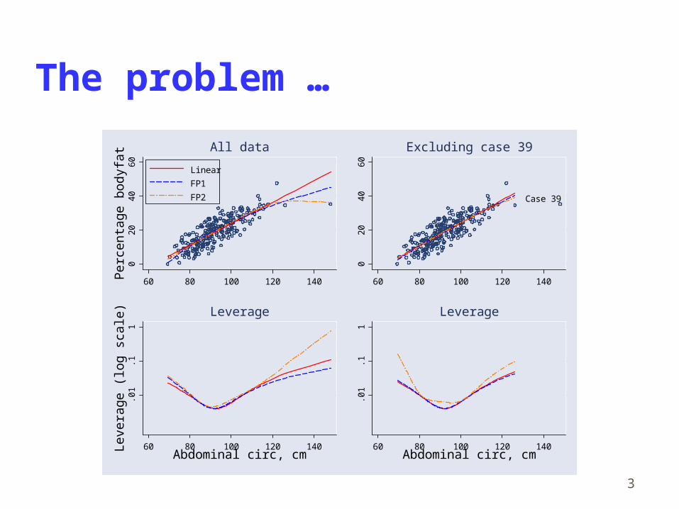
The problem …0

20

40

60

Per

cent

age

body

fat

60 80 100 120 140

Linear

FP1

FP2

All data

Case 39

02

04

06

0

60 80 100 120 140

Excluding case 39.0

1.1

1Le

vera

ge (

log

scal

e)

60 80 100 120 140Abdominal circ, cm

Leverage

.01

.11

60 80 100 120 140Abdominal circ, cm

Leverage

4

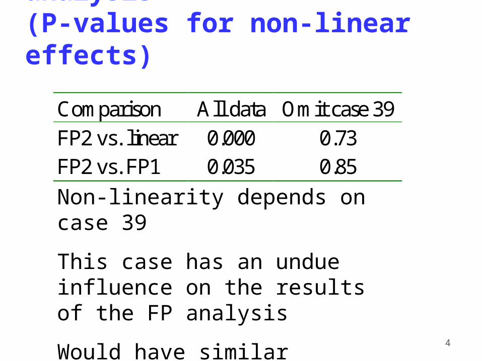
Effect of case 39 on FP analysis(P-values for non-linear effects)

Comparison All data Omit case 39 FP2 vs. linear 0.000 0.73 FP2 vs. FP1 0.035 0.85

Non-linearity depends on case 39

This case has an undue influence on the results of the FP analysis

Would have similar influence on other flexible models, e.g. splines

5

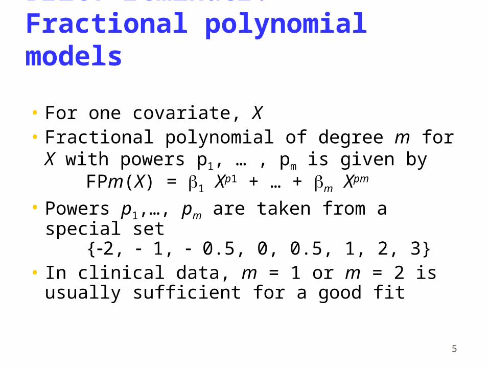
Brief reminder:Fractional polynomial models

• For one covariate, X• Fractional polynomial of degree m for X with

powers p1, … , pm is given byFPm(X) = 1 Xp1 + … + m Xpm

• Powers p1,…, pm are taken from a special set {2, 1, 0.5, 0, 0.5, 1, 2, 3}

• In clinical data, m = 1 or m = 2 is usually sufficient for a good fit

6

FP1 and FP2 models

• FP1 models are simple power transformations• 1/X2, 1/X, 1/X, log X, X, X, X2, X3

8 models of the form 0 + 1Xp

• FP2 models have combinations of the powersFor example 0 + 1(1/X) + 2(X2)28 models

• Also ‘repeated powers’ modelsFor example (1, 1): 0 + 1X + 2X log X8 models

7

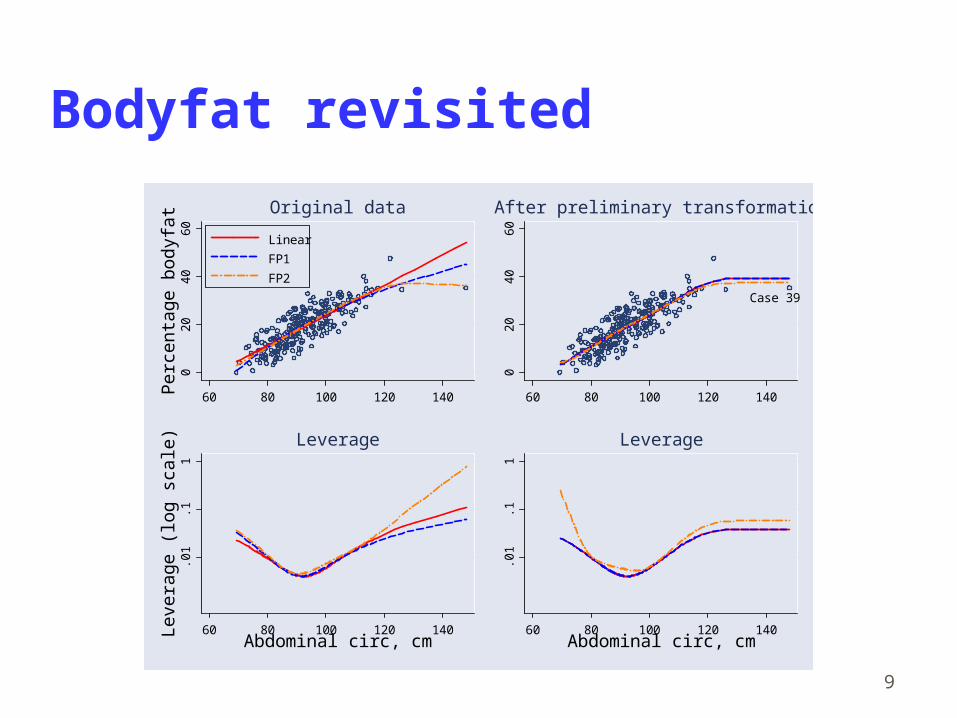
Bodyfat: Case 39 also influences a multivariable FP model

Covariate All data Case 39 omitted

Height 1 Abdomen 1 1 Biceps 3, 3 Wrist 1 1 Weight 1 Thigh -2, -2

Case 39 is extreme for several covariates

8

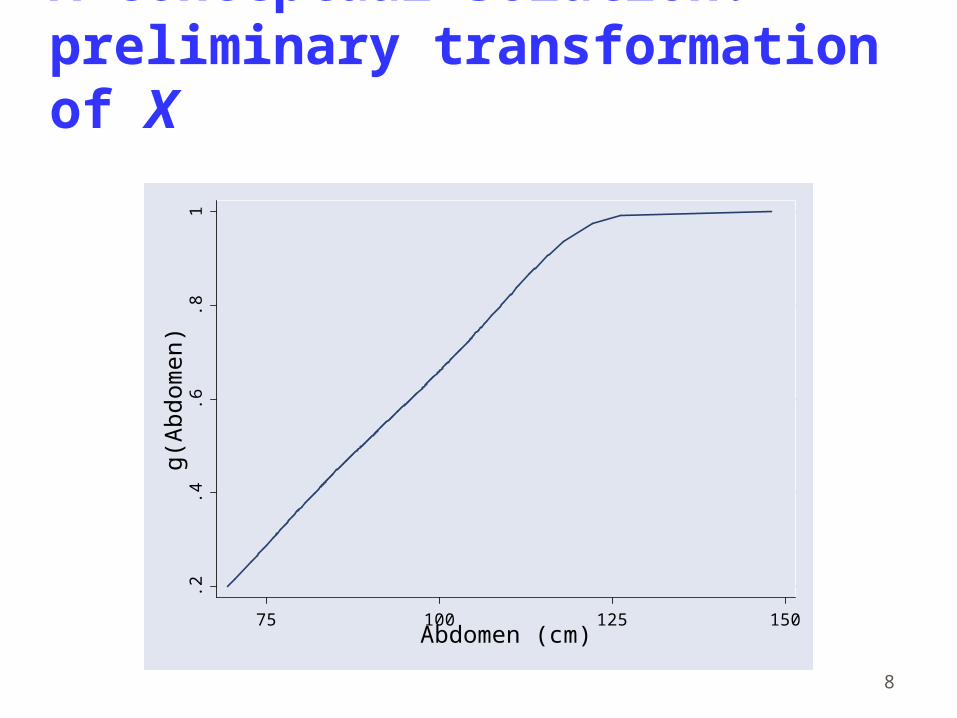
A conceptual solution:preliminary transformation of X

.2.4

.6.8

1g(

Abd

omen

)

75 100 125 150Abdomen (cm)

9

Bodyfat revisited0

20

40

60

Per

cent

age

body

fat

60 80 100 120 140

Linear

FP1

FP2

Original data

Case 39

02

04

06

0

60 80 100 120 140

After preliminary transformation.0

1.1

1Le

vera

ge (

log

scal

e)

60 80 100 120 140Abdominal circ, cm

Leverage

.01

.11

60 80 100 120 140Abdominal circ, cm

Leverage

10

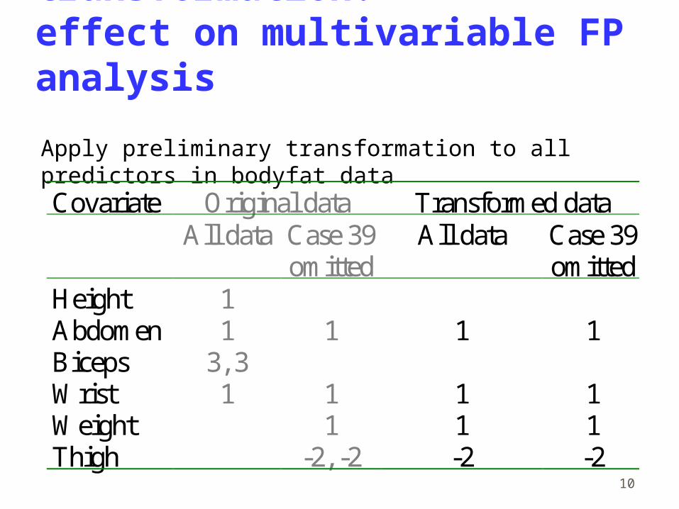
Preliminary transformation:effect on multivariable FP analysis

Apply preliminary transformation to all predictors in bodyfat data

Covariate Original data Transformed data All data Case 39

omitted All data Case 39

omitted Height 1 Abdomen 1 1 1 1 Biceps 3, 3 Wrist 1 1 1 1 Weight 1 1 1 Thigh -2, -2 -2 -2

11

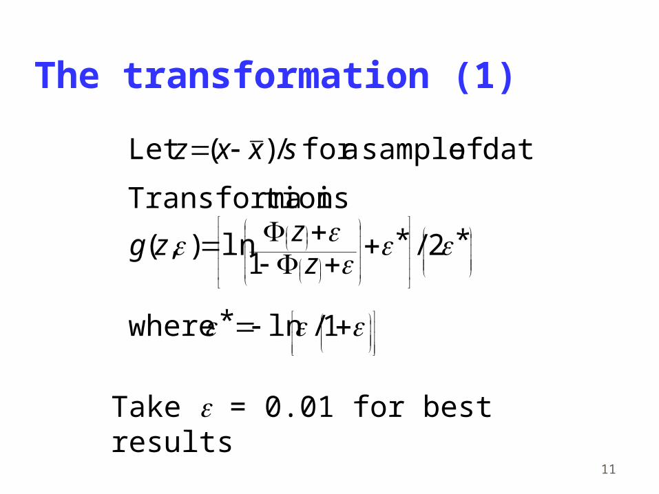
The transformation (1)

1/ln* where

*2/*1

ln),(

istion Transforma

data of sample afor /)(Let

zzzg

sxxz

Take = 0.01 for best results

12

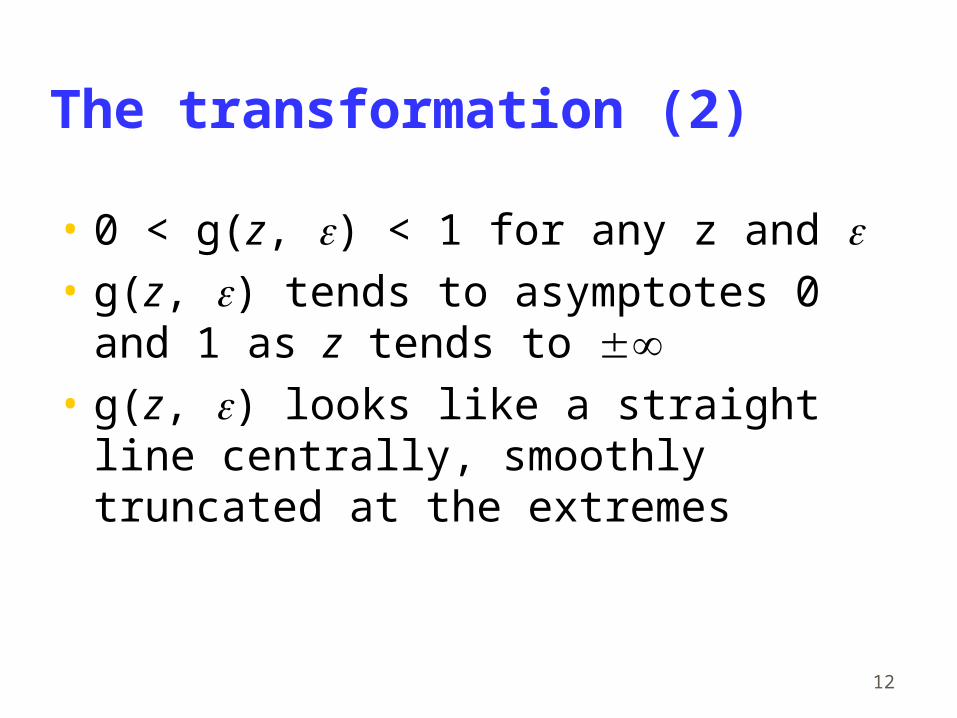
The transformation (2)

• 0 < g(z, ) < 1 for any z and • g(z, ) tends to asymptotes 0 and 1 as z tends

to • g(z, ) looks like a straight line centrally,

smoothly truncated at the extremes

13

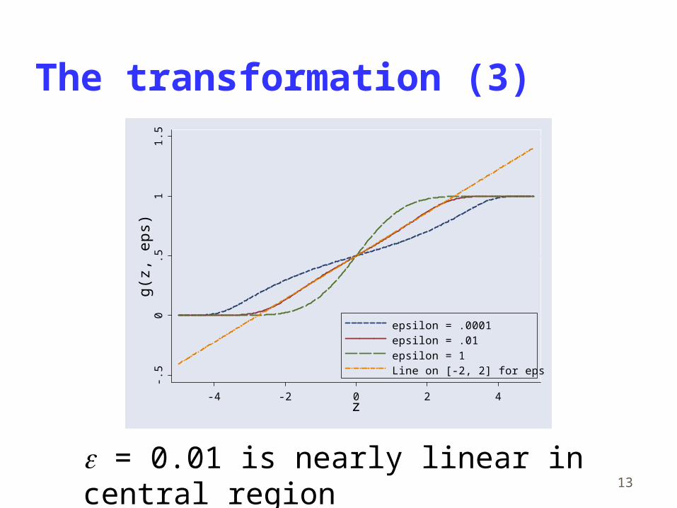
The transformation (3)

= 0.01 is nearly linear in central region

-.5

0.5

11.

5g(

z, e

ps)

-4 -2 0 2 4z

epsilon = .0001epsilon = .01

epsilon = 1Line on [-2, 2] for eps = 0.01

14

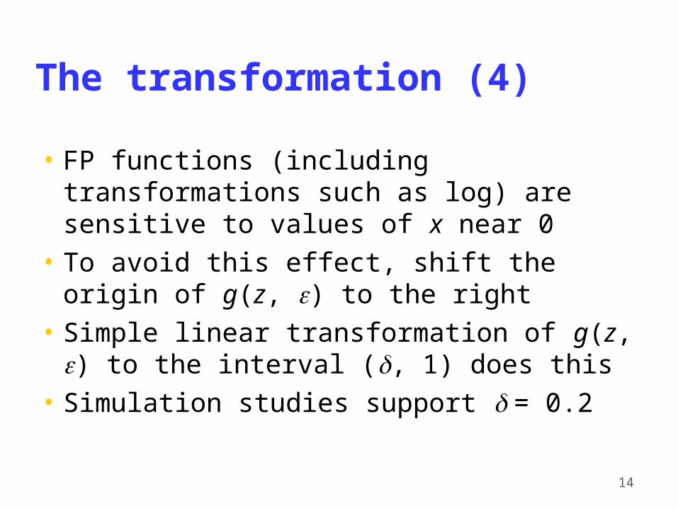
The transformation (4)

• FP functions (including transformations such as log) are sensitive to values of x near 0

• To avoid this effect, shift the origin of g(z, ) to the right

• Simple linear transformation of g(z, ) to the interval (, 1) does this

• Simulation studies support = 0.2

15

Example 2 – Whitehall 1 study

17,370 male Civil Servants aged 40-64 years• Covariates: age, cigarette smoking, BP,

cholesterol, height, weight, job grade• Outcomes of interest: all-cause mortality

logistic regression• Interested in risk as function of covariates• Several continuous covariates• Risk functions preliminary transformation

16

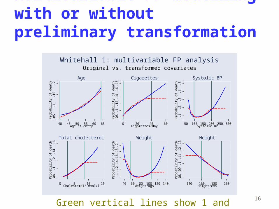
Multivariable FP modelling with or without preliminary transformation

.05

.1.1

5.2

Pro

babi

lity

of d

eath

40 45 50 55 60 65Age at entry

Age

.08

.1.1

2.1

4.1

6.1

8P

roba

bilit

y of

dea

th

0 20 40 60Cigarettes/day

Cigarettes

.1.2

.3.4

.5P

roba

bilit

y of

dea

th

50 100 150 200 250 300Systolic BP

Systolic BP

.08

.1.1

2.1

4.1

6P

roba

bilit

y of

dea

th

0 5 10 15Cholesterol/ mmol/l

Total cholesterol

.1.1

2.1

4.1

6.1

8.2

Pro

babi

lity

of d

eath

40 60 80 100 120 140Weight/kgs

Weight

.08

.09

.1.1

1.1

2.1

3P

roba

bilit

y of

dea

th

140 160 180 200Height/cms

Height

Original vs. transformed covariatesWhitehall 1: multivariable FP analysis

Green vertical lines show 1 and 99th centiles of X

17

Comments and conclusions

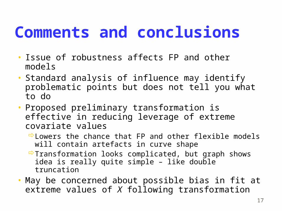
• Issue of robustness affects FP and other models• Standard analysis of influence may identify

problematic points but does not tell you what to do• Proposed preliminary transformation is effective in

reducing leverage of extreme covariate valuesLowers the chance that FP and other flexible models will

contain artefacts in curve shapeTransformation looks complicated, but graph shows idea is

really quite simple – like double truncation

• May be concerned about possible bias in fit at extreme values of X following transformation