Embed Size (px)
Citation preview
1
Making Do With Less: Working Harder During Recessions
Edward P. Lazear*
Kathryn L. Shaw**
Christopher Stanton***
October 25, 2014
Abstract
Why did productivity rise during recent recessions? One possibility is that average
worker quality increased. A second is that each incumbent worker produced more. The
second effect is termed “making do with less.” Using data from 2006 to 2010 on
individual worker productivity from a large firm, these effects can be measured and
separated. For this firm, most of the gain in productivity during the recession was a result
of increased effort. Additionally, the increase in effort is correlated with the increase in
the local unemployment rate, presumably reflecting the costs of losing a job.
* Graduate School of Business and Hoover Institution, Stanford University,
**Stanford University, Graduate School of Business.
*** London School of Economics, Department of Management.
We are grateful for comments from Darrell Duffie, Michael Powell, James Spletzer, participants
at the NBER conference Labor Markets After the Great Recession, the Trans-Pacific Labor
Studies conference, the AEA meetings 2013, and seminar participants at Arizona State,
Northwestern Kellogg, Insead, the LSE, and UCL.

2
Productivity rose during the recent recession. From 2007 to 2009, aggregate output fell
by 7.16 percent, but the aggregate number of hours worked decreased by 10.01 percent in
nonfarm business.1 Input fell by more than output, which implies that productivity increased.
More surprising, the growth in productivity during the recession outstripped the growth in
productivity both in the period directly preceding and the period directly following the recession.
From 2007 quarter 4, the start of the recession, to 2009 quarter 3, the quarter following the
recession, labor productivity rose by 3.16% in nonfarm businesses. From 2006 quarter 1 through
2007 quarter 3 productivity rose by only 2.21%.
There are two obvious possibilities that can account for the rise in productivity. The first
is that the decline in the workforce resulted in average worker quality that was higher during the
recession than in the preceding period. The second is that each worker produced more while
holding worker quality constant. This effect is termed “making do with less,” that is, getting the
same output from fewer workers.
There are both theoretical and empirical questions that need to be answered. The most
important empirical issue is determining how much of the increase in productivity is explained
by increased effort, and how much can be explained by compositional effects, i.e., having better
workers on average during the recession.2
1 The recession was from December 2007 through June 2009. The drop in output and aggregate number of hours
worked are measured from the fourth quarter 2007, the start of the recession, through the third quarter 2009, the
quarter following the recession. Data come from the BLS and exclude farm workers. 2 Other research makes reallocation – either of workers or of firms – the source of rising productivity over the cycle.
Berger (2012) argues that labor productivity rises in recessions because firms restructure during recessions by
laying off their least productive workers. His aim is to explain the jobless recoveries in the last three recessions,
pointing out that output grows but employment lags because the workers are more productive. His evidence comes
from a calibration exercise in which he compares his model to several alternative models of the business cycle,
finding that the labor restructuring model has the greatest explanatory power. Thus, labor restructuring is a
3
The most important theoretical issue involves modeling the change in effort that a firm
may require as the economy moves from normal times into recession. Intuitively, it seems that
employers push their employees harder during recessions as they cut back the work force and ask
each of the remaining workers to cover the tasks previously performed by the now-laid-off
workers. But if it is possible to get more from employees during recessions, why don’t
employers demand the higher level of output during normal times?
There are two conceptual reasons for the rise in productivity. First, during recessions,
demand for labor falls, which reduces the wage and other alternatives available to each worker.
As a consequence, workers, especially those whose next best alternative is now leisure, may be
willing to work harder for a given wage. The supply of effort to a given firm depends on a
worker’s alternatives and, as alternatives become poorer, the supply to a given firm may
improve.3 Even for the market as a whole, the reservation value of effort may decline when the
number of jobs declines as workers are forced into poorer alternatives.
Second, the labor force may change average quality for the same reason. There is no
reason to assume that workers of all ability levels are affected equally by the recession. To the
extent that some are hurt more than others, the willingness to supply effort to a given firm (or the
labor market in general) may be altered differentially across groups. Consequently, firms move
candidate explanation for productivity growth (see also Koenders and Rogerson, 2005, Gali and van Rens, 2010,
and van Rens, 2004, for models of the rising pro-cyclicality of productivity). Reallocation of workers across
businesses can also explain why some businesses are more productive than others in the cross-section (Syverson,
2011).
3 See Davis, Faberman, and Haltiwanger (forthcoming) for model and results showing that the rate at which
establishments fill jobs rises with the use of instruments such as advertising, screening methods, hiring expenditures,
and compensation packages. In high unemployment areas, where the workers’ alternatives become poorer, it may
be true that firms cut back on their use of these methods and workers are more likely to stay with their current firm.
4
in the direction of the labor type that is more cost effective and, during recessions, it is possible
that this favors higher quality workers.
Is it possible in a standard model for work effort to increase, average ability to increase,
output to fall and employment to fall when product demand falls? If there is uncertainty
associated with obtaining another job upon termination, and if work effort affects the probability
of retaining the current job, the worker will take into account the likelihood of obtaining another
job in determining his work effort. In times or areas where unemployment is high, job loss is
especially costly and effort responds accordingly. As a result, effort is expected to vary directly
with the unemployment rate, which measures the likelihood of finding a replacement job. This is
consistent with standard notions of labor supply. A worker’s willingness to supply labor (effort
or hours) increases with the wage and decreases with the alternative use of time. When the
alternatives are poorer, say because job search is less likely to result in success, it is optimal for a
worker to respond with increased effort.
This theory is taken to the data for one large firm that measures output per worker. There
is panel data on individual productivity for over 23,000 moderately skilled workers who perform
the exact same task at different establishments throughout the United States. It is therefore
possible to measure performance outcomes due to effort versus sorting using about 5.6 million
data points on daily performance from June 2006 to May 2010.
The primary finding is that effort varies over the business cycle, rising during periods of
recession. Productivity increased by 5.4 percent during the recession at this firm,
The labor force composition effect is minimal. Nearly all of the increase in productivity
that occurs during the recession is a consequence of making do with less. The quality of the
5
work force hardly changes. Instead, the increase in productivity comes about because workers
work harder. As effort increases, the task is completed in less time. Specifically, using the most
conservative estimates, composition changes account for, at most, 27 percent of the 5.4 percent
increase in productivity during the recession. This figure is obtained from the largest of three
estimates; first, a comparison of OLS productivity regressions and regressions including worker
fixed effects suggests the role of sorting is minimal. When worker fixed effects are included, the
change in productivity that is associated with the recession reflects only increased effort for a
given worker, averaged across all workers. Second, estimates from a balanced panel of workers
who were employed throughout the entire period similarly show that productivity for these
workers rose by 4.8 percent, slightly less than the increase in productivity for the entire sample.
A final analysis compares mean differences in productivity for workers who stay and workers
who leave; accumulated attrition accounts for a 1 percent change in productivity over the whole
recession while new hires increased aggregate productivity by 0.45 percent. Composition
changes, estimated with minimal functional form assumptions in this way, account for 1.45/5.4 =
27 percent of the increase in productivity during the recession.
More compelling evidence for the increased-effort effect is that effort varies across
establishments within the firm even at a point in time. Worker effort is highest at establishments
that are located in high unemployment areas; this is true even after accounting for persistent
differences in productivity between establishments. There is strong cross-sectional variation in
worker effort that is directly related to local unemployment rates. At a given point in time, those
establishments that are in high unemployment areas are also those at which worker effort is high.
At a given establishment, workers increase their effort during periods of high unemployment.
6
Additionally, it is the least productive workers in the pre-recession period who increased
their effort most in response to the local unemployment rate. If low productivity workers are the
ones least likely to find a replacement job when unemployment rates rise, then, as the model
shows, it would be logical for low productivity workers to increase their effort most.
I. Theory
A Rational Model of Changes in Effort and Ability During Recessions
Recall that the goal is to understand within the framework of rational firms how effort
might rise during recessions and how the optimal quality of workers employed might also vary
with business cycle conditions. During recessions output falls (or at a specific growing firm,
output growth slows), employment falls (or in a specific growing firm, employment growth
slows), output-per-worker rises and average ability of the work force may change. The firm
makes do with less. An additional feature (observed empirically during the last recession) is that
costs fell and profits rose, because cost saving was sufficiently great to offset the reductions in
demand.
The goal is to provide a theoretical structure that allows all the empirical phenomena to
be captured. The following model accomplishes that. 4
The Choice of Effort Level
Worker quality is indexed by k, where higher levels of k are associated with more able
workers. The cost of effort for any type k is given by c(e) / k .
4 See also Lazear (2000a) for an earlier model of optimal effort and compensation choice in an environment of
heterogeneous worker ability.
7
The timing, which we believe realistically captures the nature of the typical labor
contract, is as follows. The firm calls out the terms of employment, which consist of a wage W,
and minimum level of effort (or output) requirement, x, which has distribution function G(x) and
density g(x).5 The worker does not know x precisely, but knows the distribution of requirements
in the population of firms. At the time of hiring, market conditions that will prevail in the future,
specifically, the level of the unemployment rate, are unknown. After the worker begins the job,
the state of the economy becomes known. If effort falls below the required level, the worker is
fired. A terminated worker may find another job, which yields rent net of effort, equal to R.
Rent R is positive and dominates unemployment, but is lower than the surplus (derived below)
that is obtainable at the optimal level of effort on the primary job. If the worker does not locate a
new job, he becomes unemployed, which has value normalized to zero. Thus, the expected rent
of a terminated worker is given by (1-u)R where u is the probability that a terminated worker
remains unemployed. No theory of unemployment is presented here; u is taken as given and
exogenous, which it is for any particular worker.
The tradeoff for the worker is that effort is painful, but the higher the level of effort, the
less likely is the worker to be terminated for poor performance. The probability of being
terminated given any effort level e is merely the probability that effort, e, falls below required
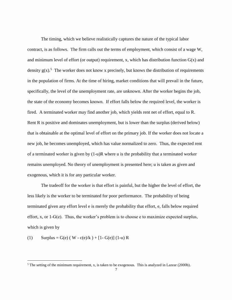
effort, x, or 1-G(e). Thus, the worker’s problem is to choose e to maximize expected surplus,
which is given by
(1) Surplus = G(e) ( W - c(e)/k ) + [1- G(e)] (1-u) R
5 The setting of the minimum requirement, x, is taken to be exogenous. This is analyzed in Lazear (2000b).

8
The first term is the probability of surviving in the firm times expected rent at that firm. The
second term is the expected rent associated with termination.6
The first-order condition for (1) is
(2) ∂/∂e = g(e) [W - c(e)/k - (1-u) R] - G(e) c’(e)/k = 0
with second-order condition ∂2/∂e2 < 0 for an interior maximum.
The first result is that effort increases in k. The more able individuals put forth higher
levels of effort because the cost of reducing the probability of termination is decreasing in
ability. That follows directly from (2) using the implicit function theorem.
e
k
k
eF O C|
/
/. . .
or
e
k
k
e
g e c e k G e c e k
e
F O C|/
/
( ) ( ) / ( ) ' ( ) /
/
. . .
2 2
2 2
2 2
which is positive because the numerator is positive and the denominator is the second-order
condition, which must be negative for the solution to the problem to be a maximum.
6 Note that the contract here is one of a fixed wage, rather than a piece rate. One could envision that the firm would
condition payment on the ex post observed level of output, e, especially since that is assumed to be known after
work occurs. Indeed, in the jobs that we have in mind, e is easily measured and tracked by a computer. The
analysis of whether to use a fixed wage or a piece rate is first laid out in Lazear (1986). There, issues of
measurement costs and multi-tasking (defined as the tradeoff between quality and quantity) are discussed. For the
purposes here, it is taken as given (and is true) that the firm does not use variable pay to any significant extent.
9
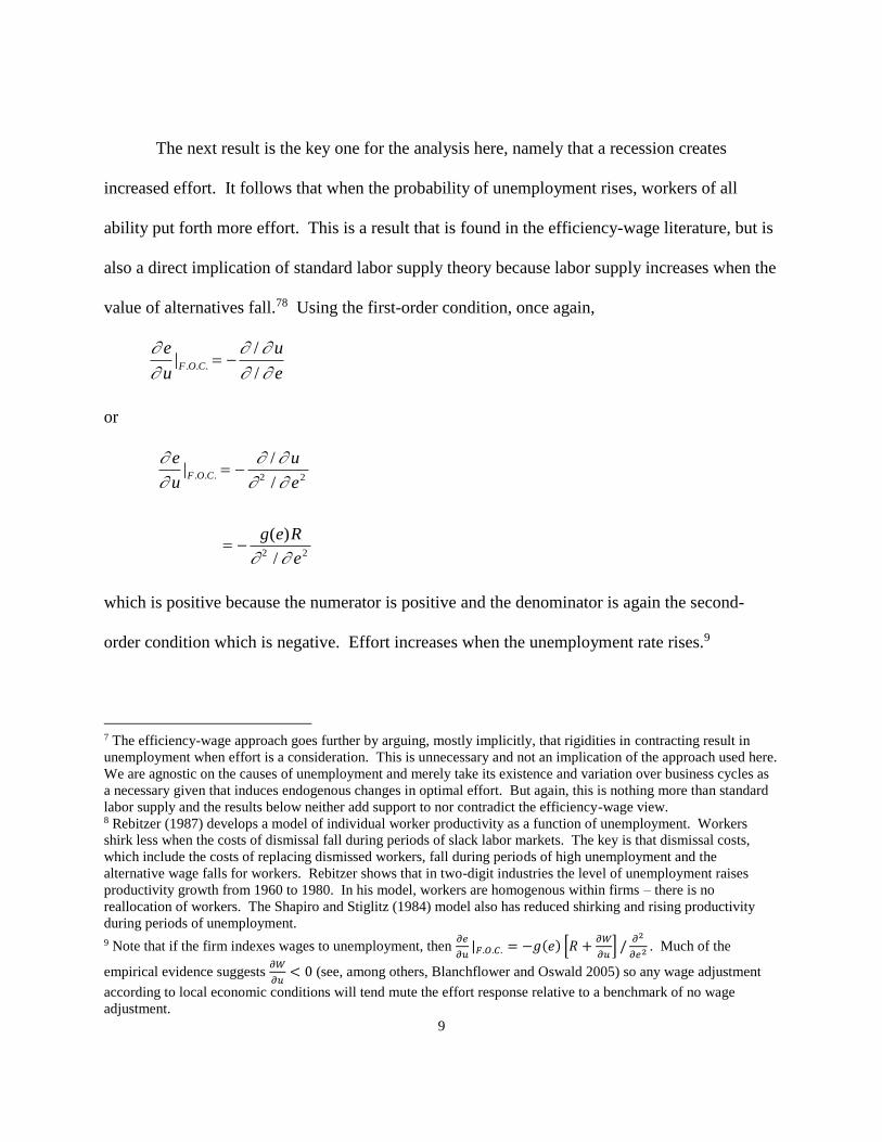
The next result is the key one for the analysis here, namely that a recession creates
increased effort. It follows that when the probability of unemployment rises, workers of all
ability put forth more effort. This is a result that is found in the efficiency-wage literature, but is
also a direct implication of standard labor supply theory because labor supply increases when the
value of alternatives fall.78 Using the first-order condition, once again,
e
u
u
eF O C|
/
/. . .
or
e
u
u
e
g e R
e
F O C|/
/
( )
/
. . .
2 2
2 2
which is positive because the numerator is positive and the denominator is again the second-
order condition which is negative. Effort increases when the unemployment rate rises.9
7 The efficiency-wage approach goes further by arguing, mostly implicitly, that rigidities in contracting result in
unemployment when effort is a consideration. This is unnecessary and not an implication of the approach used here.
We are agnostic on the causes of unemployment and merely take its existence and variation over business cycles as
a necessary given that induces endogenous changes in optimal effort. But again, this is nothing more than standard
labor supply and the results below neither add support to nor contradict the efficiency-wage view. 8 Rebitzer (1987) develops a model of individual worker productivity as a function of unemployment. Workers
shirk less when the costs of dismissal fall during periods of slack labor markets. The key is that dismissal costs,
which include the costs of replacing dismissed workers, fall during periods of high unemployment and the
alternative wage falls for workers. Rebitzer shows that in two-digit industries the level of unemployment raises
productivity growth from 1960 to 1980. In his model, workers are homogenous within firms – there is no
reallocation of workers. The Shapiro and Stiglitz (1984) model also has reduced shirking and rising productivity
during periods of unemployment.
9 Note that if the firm indexes wages to unemployment, then 𝜕𝑒
𝜕𝑢|𝐹.𝑂.𝐶. = −𝑔(𝑒) [𝑅 +
𝜕𝑊
𝜕𝑢] /
𝜕2
𝜕𝑒2 . Much of the
empirical evidence suggests 𝜕𝑊
𝜕𝑢< 0 (see, among others, Blanchflower and Oswald 2005) so any wage adjustment
according to local economic conditions will tend mute the effort response relative to a benchmark of no wage
adjustment.
10
The same analysis also implies that higher wages induce more effort because u and W
enter in the same way in (2).
Which workers increase their effort the most? The first-order effect comes through
differential changes in unemployment rates. As an empirical matter, the increase in
unemployment during recessions tends to be concentrated among the less skilled. That is not
quite the same as ability as it is measured here, but if the least talented are more likely to see a
rise in unemployment than the most talented, the increase in effort should be greater for the least
talented. Another implication is that those regions or industries that experience the largest
increase in unemployment during recessions should also witness the largest increase in effort.
That implication is not completely unambiguous because the result depends not only on
which group experiences the greatest increase in unemployment, but also on which group
responds the most to a given increase in unemployment. To get at this, it is necessary to sign
∂(∂e/∂u) / ∂k and the response of effort to a change in unemployment may be increasing in k.
This is shown in the appendix. The implication as to which group increases effort more in a
recession is somewhat ambiguous. Still, there is one clear implication with respect to
unemployment.
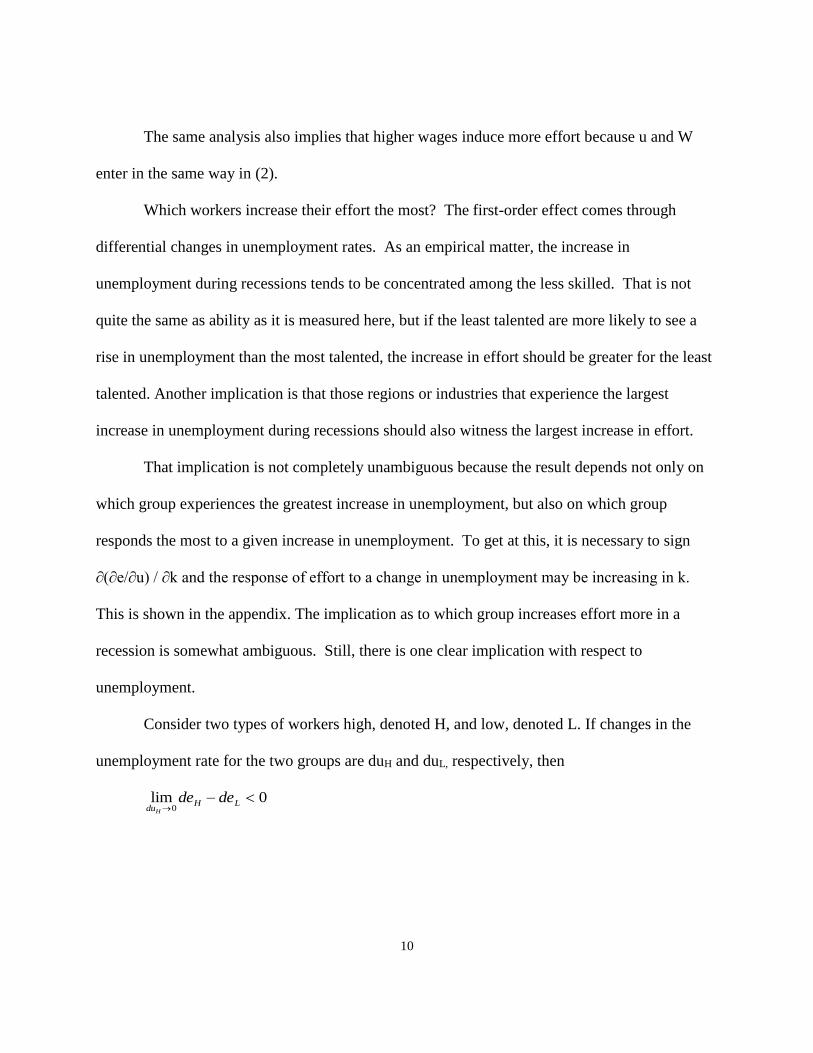
Consider two types of workers high, denoted H, and low, denoted L. If changes in the
unemployment rate for the two groups are duH and duL, respectively, then
lim
duH L
H
de de
0
0
11
As the change in unemployment for the skilled gets small relative to that for the unskilled, the
change in effort for the unskilled exceeds that for the skilled. Thus, as long as uL rises enough
relative to uH, the unskilled will increase their effort by more than the skilled.
Although the relative increase in effort across skill groups during recessions remains an
empirical question, the implication from the logic above is that at least for large differences
between the increase in unemployment among the low ability and high ability types, the
expectation is that low ability workers should increase their effort more than high ability
workers.
Composition Effects
How does employment vary with market conditions? In order to ascertain this, it is
necessary to present a model of hiring and determine which workers are retained when market
conditions are worse than expected.10
The firm knows the worker’s behavior as determined by (1) and (2). Recall that R is the
rent that a worker receives on the alternative job. Using (1), a worker accepts the job if
(3) G(e) ( W - c(e)/k ) + [1- G(e)] (1-u) R > 0
Recall that u is unknown at the time of hire so the worker decides whether to accept the job
based on the expectation of u.
Condition (3) implies that there is some k* below which the worker will not accept the
job so the workers who are successfully hired by the firm are those for whom k>k*.11 Suppose
10This analysis is based on the model presented in Lazear (2000a). 11 There could also be an upper cutoff. This arises when R depends on k and R rises sufficient with k so that high
ability workers find that the rent that they receive on the alternative job exceeds that on the one being offered.
12
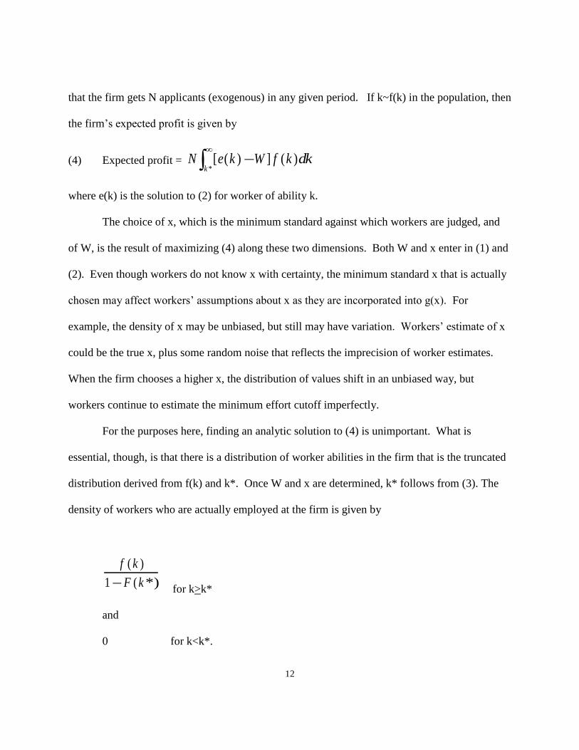
that the firm gets N applicants (exogenous) in any given period. If k~f(k) in the population, then
the firm’s expected profit is given by
(4) Expected profit = N e k W f k dkk
[ ( ) ] ( )*
where e(k) is the solution to (2) for worker of ability k.
The choice of x, which is the minimum standard against which workers are judged, and
of W, is the result of maximizing (4) along these two dimensions. Both W and x enter in (1) and
(2). Even though workers do not know x with certainty, the minimum standard x that is actually
chosen may affect workers’ assumptions about x as they are incorporated into g(x). For
example, the density of x may be unbiased, but still may have variation. Workers’ estimate of x
could be the true x, plus some random noise that reflects the imprecision of worker estimates.
When the firm chooses a higher x, the distribution of values shift in an unbiased way, but
workers continue to estimate the minimum effort cutoff imperfectly.
For the purposes here, finding an analytic solution to (4) is unimportant. What is
essential, though, is that there is a distribution of worker abilities in the firm that is the truncated
distribution derived from f(k) and k*. Once W and x are determined, k* follows from (3). The
density of workers who are actually employed at the firm is given by
f k
F k
( )
( *)1 for k>k*
and
0 for k<k*.
13
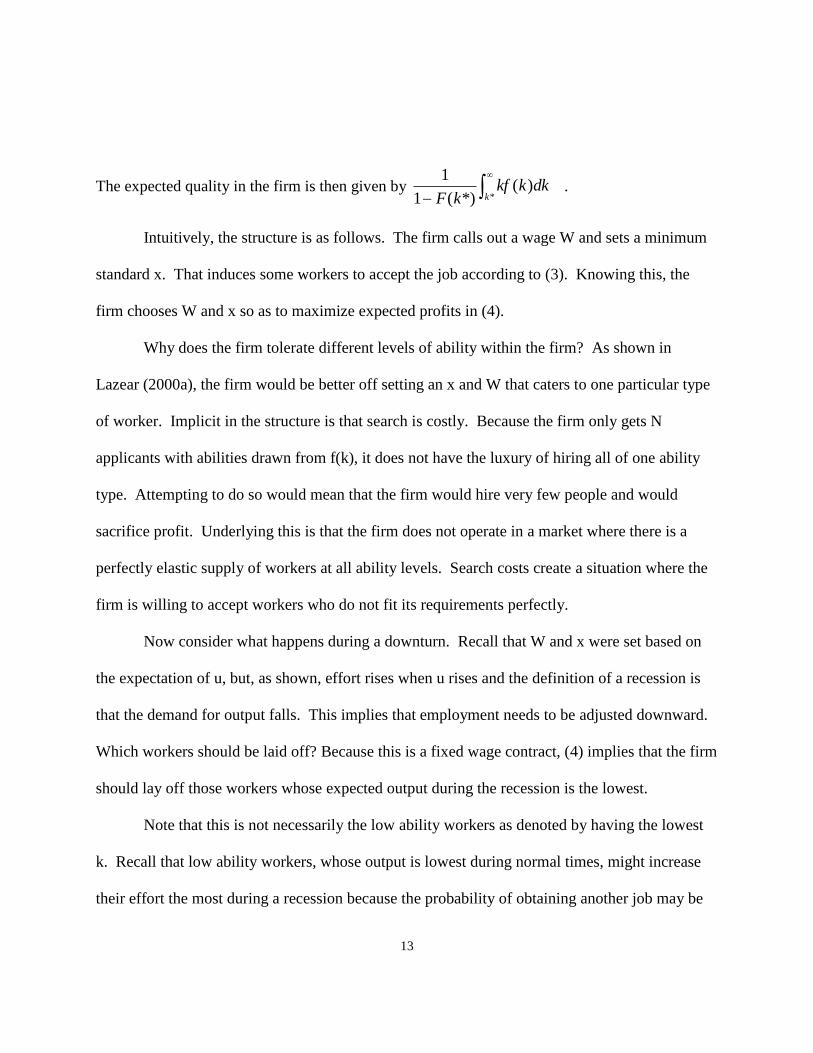
The expected quality in the firm is then given by 1
1
F kkf k dk
k( *)( )
* .
Intuitively, the structure is as follows. The firm calls out a wage W and sets a minimum
standard x. That induces some workers to accept the job according to (3). Knowing this, the
firm chooses W and x so as to maximize expected profits in (4).
Why does the firm tolerate different levels of ability within the firm? As shown in
Lazear (2000a), the firm would be better off setting an x and W that caters to one particular type
of worker. Implicit in the structure is that search is costly. Because the firm only gets N
applicants with abilities drawn from f(k), it does not have the luxury of hiring all of one ability
type. Attempting to do so would mean that the firm would hire very few people and would
sacrifice profit. Underlying this is that the firm does not operate in a market where there is a
perfectly elastic supply of workers at all ability levels. Search costs create a situation where the
firm is willing to accept workers who do not fit its requirements perfectly.
Now consider what happens during a downturn. Recall that W and x were set based on
the expectation of u, but, as shown, effort rises when u rises and the definition of a recession is
that the demand for output falls. This implies that employment needs to be adjusted downward.
Which workers should be laid off? Because this is a fixed wage contract, (4) implies that the firm
should lay off those workers whose expected output during the recession is the lowest.
Note that this is not necessarily the low ability workers as denoted by having the lowest
k. Recall that low ability workers, whose output is lowest during normal times, might increase
their effort the most during a recession because the probability of obtaining another job may be
14
related to k. As a result, although the composition of the workforce should change in the
direction of higher effort workers, this does not necessarily imply that one can predict which
workers are to be laid off based on their pre-recession levels of output. It is the ex post effort
that matters so there is not an unambiguous prediction of how layoffs or composition of the work
force should relate to the fixed effects that are estimated before the recession.
The implication of this section is that effort rises unambiguously for each worker who is
retained and the composition of the workforce should shift toward those who will be most
productive during the recession, but this is not necessarily those who were most productive
before the recession.
II. Data
The data consist of daily productivity measures from a large services company. The jobs
in the company are what we label “technology based service” jobs or “TBS jobs.”
Confidentiality restrictions limit our ability to reveal the exact nature of the work. Examples of
TBS jobs include insurance-claims processing, computer-based test grading, technical call
centers, retailing jobs such as cashiers, movie theater concession stand employees, in-house IT
specialists, airline gate agents, technical repair workers, and a large number of other jobs.
These jobs have a common defining feature: a computer tracks the productivity of each
individual worker. Many production processes in services now fit this description, and TBS jobs
are widespread. The technology that is used to measure performance may be a new computer-
based monitoring system such as an ERP (Enterprise Resource Planning) system that records a
worker’s productivity each day (such as the number of windshield repair visits done by each
Safelite® worker (Lazear, 2000b; Shaw and Lazear, 2008)), cash registers that record each
15
transaction under an employee ID number, call centers, or computer-monitored data entry.
The data contain four years of daily productivity transaction records between June 2006
and May 2010. There are 23,580 unique workers for a total worker-day sample size of about 5.6
million observations.12 The data come from many establishments spanning a large number of
states, but the number of establishments and the exact number of states cannot be revealed for
confidentiality reasons.13
Many of the empirical results exploit the fact that workers in different locations
experienced different unemployment rates over the business cycle. Importantly, at any point in
time, the company did not change the nature of the task or the task assignment process across
establishments. This company has multiple different service functions, but, for the productivity
measure used here, the data come from one task classification where workers are involved in
general transactions. This ensures that all workers in the sample perform the exact same
expected task across establishments. In addition, the output from the task is geographically
portable, so local demand conditions do not affect task assignment. During the sample period,
the task assignment process remained constant, and the company did not change the task
distribution in response to local labor market conditions or local demand for the service.
In this company, the productivity of the worker is controlled by the worker’s effort.
Because the job is discrete, as in the case of a windshield repair as analyzed in the Safelite study
(where a job consists of installing one windshield), productivity depends solely on the speed with
12 The data also contain information on each worker’s boss, or supervisor. The quality of the supervisor also
influences the productivity of the worker, as is emphasized in Lazear, Shaw, and Stanton (2015). There are 1,630
bosses. 13 To study the effect of the recession on productivity, we restrict the data to locations with sufficient operating
history prior to the recession. We also drop the data from the first month of operations for new establishments.
16
which the worker performs the task. Although each assigned job may vary in difficulty, in
expectation every job assignment is the same. Additionally, downtime is minimized by altering
the total number of workers at any point in time. In fact, workers are sent home when there are
too many to accommodate demand.
The information technology system measures the time it takes to process a customer
transaction from beginning to end. If there is slack time because there are no customers, this
downtime is not measured. Productivity is, therefore, the average number of transactions a
worker handles in an hour, when the hour working is measured from total processing time. 14
The worker can increase his transactions by processing customers more quickly.
This definition of productivity is better than most for measuring effort since it is not
directly affected by demand conditions. The measure of productivity that is used here does not
vary with slack time. Because productivity is defined as the reciprocal of time taken to complete
the average job assignment, down time between jobs does not directly affect the measure. In this
respect, it differs from the macro productivity measures that compute output per unit of clock
time on the job, not actual working time on the job. As a consequence, the measure used here
does not capture productivity declines during recessions that may be associated with labor
hoarding. In the recessions that characterized the earlier periods (the 1980s and before) and those
in other countries, labor productivity falls because hours worked fall by a smaller percentage
than output. The measure used here, however, is a direct measure of effort because it nets out any
slack. It is not completely devoid of slack time considerations, however, because the amount of
slack time could affect effort during those periods when work occurs, say because more slack
14 There is no data on the number of hours the worker is scheduled to work per day.

17
allows workers to increase their speed when they are actually working. In the production context
analyzed here, this is not a major problem. Slack is minimal in all times because of the work
assignment algorithm. Additionally, a measure of slack time exists and is discussed later.
For our purposes, the measure used, which abstracts from slack time, is exactly the
correct measure. Our goal is to determine whether firms make do with less because workers step
up their effort level during recessions. If the speed at which they actually work responds to
recession and unemployment pressure, then the mechanism that we have in mind is operating.
This does not necessarily imply that productivity at the macro level would rise on net. It
is possible that increased slack time during a recession is sufficient to offset any increase in
speed during time actually worked, but slack due to deficient demand is most determined by the
employer. If productivity rises at the aggregate level despite the possibility of increased slack,
then it must be because productivity during time actually worked rises, which is exactly what is
tested using the data from this particular firm.
One final fact is worthy of note. Workers in this firm are paid an hourly wage rate. The
data do not contain workers’ wages, but the firm has a common set of human resources policies
across establishments.15 While the firm could pay for performance since output is monitored
carefully, they do not do so.
III. Empirical Results
Summary Statistics
The first finding is that there is an increase in productivity during the recession and post-
15 Front-line supervisors have limited discretion to alter wages; to the extent that management adjusted wages in
response to unemployment or local labor market conditions, the resulting estimates are likely to be understated.
18
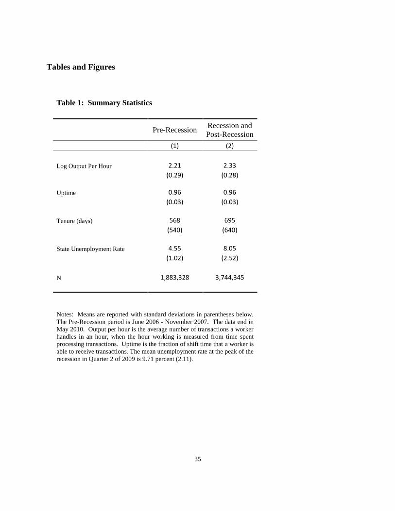
recession period. As shown in Table 1, log output per hour rises from an average of 2.21 units
during the pre-recession period (June 2006 through November 2007) to an average of 2.33 units
during the recession and post-recession period. The simple averages imply that productivity rose
during the recession. Of course, these are only simple statistics and do not speak to whether the
change comes about because workers increase effort, or because the composition of workers
change. These specifics are examined later.
Two other measures of productivity are available in the data. The first is uptime, defined
as the percentage of time a worker is physically available to receive transactions during his or her
shift. Uptime captures effort as well as demand conditions. The second measure is a quality
score, taken from an audit or post-transaction survey. Summary statistics on quality are not
presented because the scale of the measure and frequency of its collection change over time.
Figure 1 shows the time path of employment. As is clear, this is a growing firm in the
pre- and post- recession period, but, as is evident from the figure, growth in employment falls
during the recession and is even negative during some months. Mean tenure rises during the
recession to 699 days, from 680 days in the non-recession period; this is consistent with the
slowdown in hiring and quitting economy-wide.1617 Figure 2 shows graphically the results
reported in Table 1 for output-per-hour. Productivity rises during the recession.
Productivity Effects of the Recession
Table 2 examines productivity during the recession in a more refined way by including
16 JOLTS (Job Opening and Labor Turnover Survey) data show significant reduction in churn in the broader
economy. 17 There are no data available on the causes of worker attrition. Attrition is defined as a worker being no longer
present on production tasks either because of promotion, firing, or voluntary exit. There is a temporary spike in
attrition in December 2007 and January 2008.

19
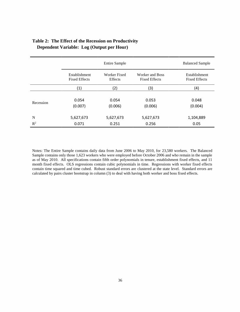
worker tenure and worker and boss effects, where appropriate.1819 The basic estimating
equation for Table 2 is
(5) log(qijt )= γ1Rt + Xitβ + ζj + εijt.
where qijt is the output per hour of worker i at establishment j at time t. The dummy variable Rt
captures the recession period from December 2007 through May 2009. The matrix Xit contains a
fifth order polynomial in workers’ tenure, a cubic polynomial in time, and 11 month dummies to
control for seasonality; ζj is an establishment fixed effect.
The overall effect of the recession is an increase in productivity of 5.4 percent, which
comes from column 1 of Table 2. There is a sizable jump in productivity, holding constant
seasonal and location-specific effects as well as those which reflect trend changes in
productivity.
As mapped out in the theory, there are two channels through which productivity can
increase during recessions. First, a given worker may put forth more effort during recessions.
Second, the composition of the workforce may change in the direction of higher quality workers
being employed during recessions. This is an empirical question. Does the increase in
productivity during the recession come from people on the job working harder or from the
attraction and retention of higher caliber people? Estimating productivity equation (5) with a
person fixed effect sheds light on this question.20
A worker fixed effect, αi, is added to the productivity regression in column 2 of Table 2.
18 See Lazear, Shaw and Stanton (forthcoming) for a discussion of the importance of boss effects. 19 Because we model the productivity of workers within establishments, we need not control for the restructuring of
firms that involves the closing of the least productive establishments during recessions (Davis and Haltiwanger,
1990; Garin, Pries and Sims, 2011; Rebitzer, 1987). 20 The methods follow those of Lazear (2000b).
20
If more productive individuals are employed during the recession due to compositional shifts in
the workforce, there will be a positive correlation between Rt and αi and the estimate of γ1 will
decline when worker fixed effects are added to the regression. The productivity gains appear to
be from increased effort, not sorting. During the recession, productivity rises by 5.4 percent in
the worker fixed effects model (column 2), which is the same as the OLS estimate. There is no
evidence that the increased productivity effect is a result of changes in composition of the
workforce. Column 3 adds boss fixed effects. The results are essentially unchanged.
To test whether sorting can explain the results, note that if sorting of workers to the firm
does not change over time, regressions using a balanced sample of continuously employed
workers should produce the same estimates as the sample with the entry and exit of workers to
the firm. This is a slightly different experiment than the one performed in column 2 of Table 2.
There, fixed effects are estimated by using all workers, but those workers are not necessarily
present throughout the entire period. The balanced sample is more restrictive, using only those
workers who are employed throughout the entire sample period. The estimate is very similar.
Column 4 of Table 2 follows the 1,623 workers (with 1.1 million daily productivity measures)
for those who are continuously employed in the three phases of the pre-recession period, the
recession period, and the post-recession period. The productivity gain during the recession is
estimated as 4.8 percent, little changed from the OLS recession effect of 5.4 percent for the full
data set of 23 thousand workers.21
21 One other potential bias is the inability to account for changes in the capital stock. To the extent that the firm
increased the capital stock, the time controls should pick this up unless there was a significant increase in investment
during the recession relative to trend; this seems unlikely. Moreover, the regression contains establishment
dummies. This is important because once an establishment is built, its capital stock is likely to remain generally
21
A direct way to analyze composition is to examine whether the exit or entry of workers to
the firm is related to worker quality. To do this, a regression that includes dummies for leaving
the job or for beginning with the firm during the recession are included. The sign of the leavers
dummy is indeterminate because some leavers were laid off and are likely to be low quality, but
some are quitters who may be high quality.22 The new-hires dummy should enter positively
because better workers are available for hire during the recession at the same price.
The results are shown in (6). 23
(6) log(qijt) = 0.053 Recession - 0.0002 Left during recession +0.015 Hired during recession.
(0.001) (0.0024) (0.003)
The estimates show no quality differential for leavers, but those hired during the
recession are 1.5 percent more productive than all others. However, the new-hires impact on
productivity is small because new-hires are only 30 percent of all those working during the
recession;24 the total impact of new-hires on aggregate productivity is 1.5*.3 = .005.
The conclusion that composition explains only a small fraction of the productivity change
holds up after additional tests for worker sorting. A simple analysis is presented here, and the
appendix contains additional results that assess counterfactual productivity in the absence of
attrition. In what follows, the productivity difference between stayers and leavers is calculated
as the monthly average of productivity for those workers who stay compared with those who
fixed over time. It is especially unlikely to be correlated with changes in local unemployment rates, on which the
bulk of the conclusions rest. 22 The market may infer that those who are laid off are of lower quality (Gibbons and Katz, 1992). 23 The regression is estimated by OLS and contains the same control variables as in column 1 of Table 2. The
sample is restricted to establishments with data in the pre-recession period. It is also possible that the composition
of the workforce differs over the recession. To allow for this possibility, equation (6) was also estimated with week
fixed effects. The point estimates (standard errors) on Left during recession and Hired during recession are -0.00004
(0.0036) and 0.0089 (0.0032), respectively. 24 The ratio of observations of new-hires to all those working during the recession is about .3.
22
leave. Although it is possible to compare the distribution of fixed effects before and during the
recession, this ignores the possibility that different workers may respond differently to the
recession, as implied by the theory. As a consequence, it is better to use the raw data to estimate
the effect of composition differences. That is what is done below. For this purpose, the
productivity for workers who leave is measured in the calendar month prior to a worker’s
departure. The results suggest that attrition accounts for a relatively small portion of the
change in productivity over the recession. Figure 3 plots the instantaneous effect on total
productivity from attrition. The instantaneous effect is computed as [log(oph)Stayers,t+1 -
log(oph)Leavers,t+1] x shareLeavers, which is the mean productivity difference between workers who
remain (stayers) and workers who leave in the month prior to attrition times the share of the
workforce that leaves. The cumulative productivity effect is plotted on the right y-axis and is
calculated as the running total of all past share-weighted productivity differences between stayers
and leavers. From this calculation, at the end of the recession the total effect of attrition on
aggregate productivity is about 0.01, which is less than one-fifth of the total change in
productivity.
Productivity Effects of Varying Local Unemployment Rates
The most compelling evidence of the recession-based effort effect comes from the next
analysis of the impact of varying local unemployment rates on productivity. The theory predicts
that cross-sectional as well as time series unemployment rates should affect productivity. The
theory relates most directly to the local unemployment rate and the evidence below is consistent
with the theoretical analysis.
The theory relies on variations in workers’ alternative use of time as the impetus for the
23
effect of recessions on productivity. An increase in the unemployment rate makes finding an
alternative job more difficult, which reduces the relative cost of effort. Workers in various
establishments in the firm experienced differences in unemployment conditions over the five
years of the data. 25 Statewide variations in unemployment rates are large, not only on average,
but also as they changed during the recession. For example, in Florida, the unemployment rate
rose from 3.3% to 11.2% from June 2006 to May 2010. In Kansas, the unemployment rate rose
from 4.4% to 7.1% over the same period.
The original productivity regression (5) can be modified to make use of differences in
labor market conditions. The model is
(7) log(qijt) = γ2UnempRijt + Xitβ + ζj + αi + τt + εijt.
where UnempRijt is the monthly unemployment rate by state matched to each establishment j and
τt is a year-by-month fixed effect. The year-by-month fixed effects remove common time-series
shocks to the unemployment rate and firm productivity, so the model is identified using across-
establishment variation in the unemployment rate within a given month.
Standard errors are clustered by state. The p-values of statistical tests are computed using
a t distribution with G-2 degrees of freedom, where G is the number of states. Statistical
inference is robust to alternative techniques to correct for clustering.26
The model with establishment fixed effects, year-by-month fixed effects, and a fifth order
polynomial in tenure (column 1, Table 3) gives a point estimate of 0.008 for the unemployment
25 In work on the efficiency wage hypothesis, Cappelli and Chauvin (1991) rely on interplant variation in wage
premiums. 26 Recent papers suggest corrections for inference in settings with a small number of clusters (Cameron, Gelbach,
and Miller 2008; Donald and Lang 2007). See the note for Table 3 and the NBER working paper version of the
paper for more detail about inference.
24
rate effect. This corresponds to a 3.9% increase in productivity for a 5 percentage point increase
in the local unemployment rate, which is the size of the increase in the national unemployment
rate from just prior to the recession to the recession peak rate.27 The next two columns add
worker and boss fixed effects, respectively. The final column reports the results for the balanced
sample. The unemployment rate effect is similar across all specifications, and indicates that
individual workers increase their effort in response to worsening local labor market conditions.
In labor intensive industries that are as competitive as the industry surrounding this firm, even a
4 percent increase in productivity is sizable.
Figure 4 splits the sample into states that established relatively high and low
unemployment changes during the recession and examines the evolution of productivity over
time for each group. As is clear from the diagram, productivity rises during the recession more in
those establishments where the change in unemployment is greatest.
It is difficult to imagine any other factor that could affect worker productivity and would
vary with local unemployment rates, holding constant both establishment and time effects. The
estimates in Table 3 are obtained by examining the increase in productivity that results when
local unemployment rates are high given both the time period in which and establishment at
which the worker is employed. For this reason, Table 3 is the most direct test of the increased-
effort hypothesis. The fact that worker output goes up most in those areas that have the highest
unemployment relative to the average for a given time period and establishment is evidence that
workers are responding to the reduced likelihood of obtaining an alternative job. The estimates
27 The rate increased from about 5.0 percent to about 10.0 percent. This approximately matches the increase in the
unemployment rate in the sample, from 4.55 to 9.71.
25
are based on the entire period and do not depend on formal definitions of recession. They play
off the differences in unemployment rates relative to what would be expected for a given
establishment and given time period, recession or not.
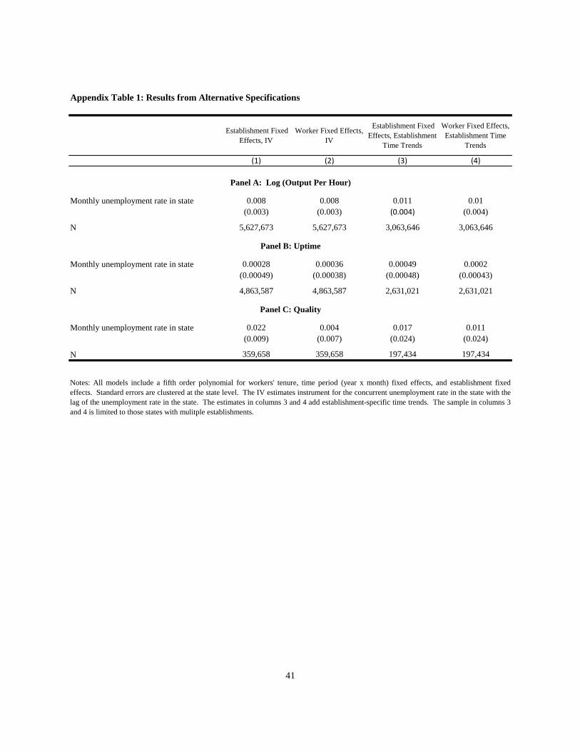
Appendix Table 1 presents several additional specifications to assess the sensitivity of the
estimates. To account for measurement error in the unemployment rate, an IV estimate using the
lagged unemployment rate as an instrument for the concurrent rate increases the parameter
estimates only slightly. The parameter estimates are also robust to the inclusion of establishment
level specific time trends for those states with multiple establishments. Results with linear trends
are presented; they are similar to results with quadratic trends.
Uptime and Quality
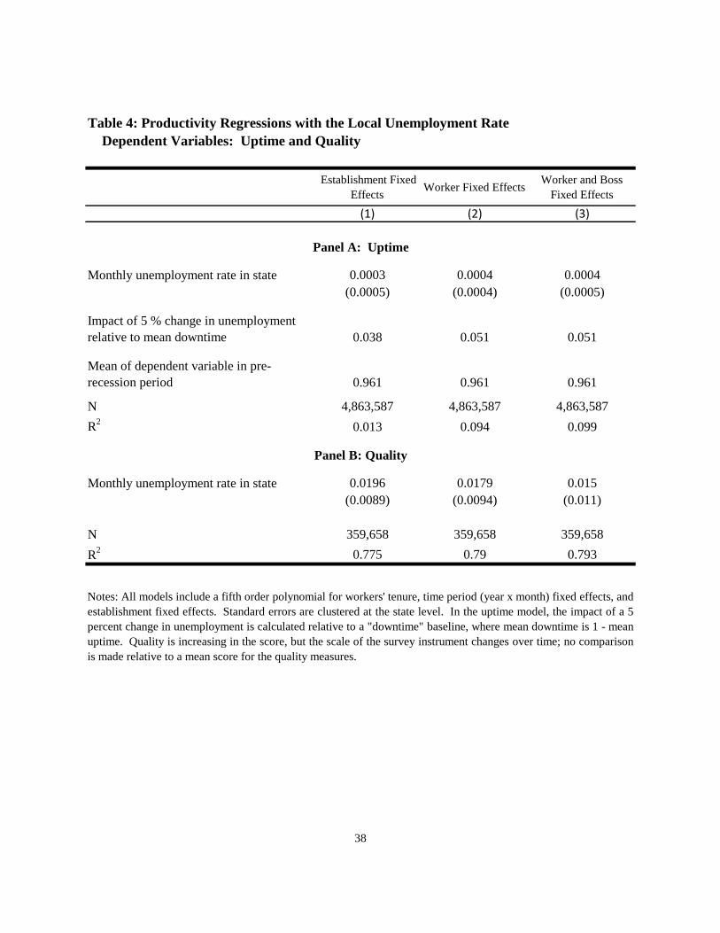
As discussed earlier, there are two additional productivity measures. Because slack time
is omitted from the output-per-hour calculation, the estimated effect corresponds directly to
effort. Uptime is an additional measure that relates more directly to slack time.
The uptime results are important for putting the interpretation of slack changes into
perspective. Interviews with the company suggest that workers are sent home in periods of high
slack, but they are expected to be at their workstation handling transactions in periods of high
demand. Uptime does not measure slack perfectly, however. Uptime measures the proportion of
time-card time during which the worker is ready to be assigned a task, but it is still possible that
time could pass between tasks.
The mean uptime in the sample is 0.963, meaning that workers are available to process
transactions for over 96 percent of their working hours. Panel A of Table 4 contains the results
from regressions with uptime as the dependent variable. The point estimates on the local
26
unemployment rate are positive but statistically insignificant in columns with establishment
effects. The results are similar when adding worker and worker and boss fixed effects. Not only
do workers increase the speed with which they perform any given task, but there is no evidence
that they increase the amount of slack time during recessions by taking more leisure on the job. If
this were the case, the coefficient on the local unemployment rate would be expected to be
negative. It remains possible, however, that total down time increases during recessions if there
were a longer time lapse between actual task assignments.
An additional measure of productivity is quality, measured from a post-transaction
assessment. Positive scores correspond to higher quality. While the scale of the quality measure
changes over time, with time fixed effects in a regression it is possible to assess whether the
output-per-hour increase due to the local unemployment rate is driven by reductions in
transaction quality. The results in Panel B of Table 4 suggest slightly positive increases in
quality with respect to the unemployment rate, mitigating concerns that multi-task considerations
drive the increased output per hour.
In summary, productivity rises when and where unemployment rates are high, reflecting
higher effort in high unemployment areas and times. Because the value of the workers’
alternatives decline with the unemployment rate, the theory predicts and results confirm that
effort should increase as unemployment rises.
Heterogeneity in the Response: Stars and Laggards
Workers need not respond equally to the recession. Two groups of workers are
considered. Define “laggards” as those who are less productive than the median worker.
Presumably, they face higher unemployment rates and lower quality future jobs. Analogously,
27
define “stars” as those who are more productive than the median. Presumably, they face lower
unemployment rates and higher quality alternative job offers. As described in the theory section,
laggards may or may not respond more to the recession than stars. The theory implies that the
less skilled group will increase their effort less for a given change in unemployment, but that
unemployment is likely to rise more for the less skilled. The predicted effect of skill level on
productivity is therefore ambiguous.
The data on workers who enter the firm in the pre-recession period are used to assess
whether stars or laggards are most responsive to the recession. Workers are classified into the
two ability categories based on their pre-recession productivity. Specifically, stars are those
workers whose worker specific fixed effect, αi, is above the median using data on workers’ first
60 days of tenure when regression (5) is estimated with a worker fixed effect for those 60 days.28
Laggards are those with below median worker fixed effect estimated in the above manner. There
are 3,121 laggards and there are 2,942 stars (the discrepancy is due to taking a median weighted
by days of work).
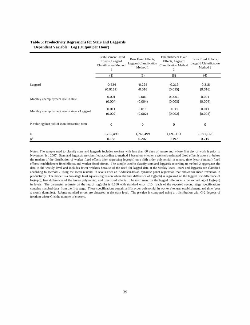
There is a significant difference in the effect of the recession on stars’ and laggards’
productivity. Laggards increase their productivity in response to increases in the local
unemployment rate by more than do stars. If the threat of unemployment and the alternative job
is poorer for laggards than for stars, one might expect that the effort of laggards would rise by
more than that for stars.
28 Workers with entry dates prior to the beginning of our sample with more than 60 days of tenure are not included.
The sample includes only workers whose first day of work is both present in the sample and occurs prior to
11/1/2007. The 11/1/2007 cutoff period is used to ensure that workers in the pre-recession estimation sample have
at least some data from which to estimate their fixed effect that is not contaminated by the recession.

28
Column 1 of Table 5 repeats the specification in Table 3. In these models, stars’ effort
response to the local unemployment rate is minimal and insignificant. Laggards, however,
increase their effort substantially. In this specification, which includes year x month and
establishment fixed effects, laggards’ productivity increases by 5.65 percent in response to a 5
percentage point increase in the local unemployment rate. Results are similar when adding boss
fixed effects.
To account for the possibility that mean reversion is driving the results, the last two
columns of Table 5 classify stars and laggards using the residuals, in levels, from an Anderson-
Hsiao dynamic panel data model estimated on weekly averages. This technique better isolates
permanent unobserved heterogeneity from state dependence or mean-reverting shocks in the
classification of stars and laggards. The results are identical.
IV. External Validity
Recall that aggregate productivity rose by 3.16 percent from the start of the recession to
the quarter following the recession. It is well known that less-educated workers experience
larger rises in unemployment during recessions than to well-educated workers. This section
assesses whether shifts in employment composition can explain a significant portion of the
productivity gain experienced during the recession.
The gain in productivity can be decomposed into that due to a shift in the composition of
the workforce to the more skilled, which for the purposes here is defined as the better educated,
versus an increase in the within education group productivity. Aggregate productivity is the
weighted sum of the within-group productivity or

29
P s pi i
where si is the share of the workforce accounted for by group i and pi is the productivity of that
group. It then follows that changes in productivity can be decomposed as
Δ𝑃 = ∑ Δ𝑠𝑖𝑝�̅� + Δ𝑝𝑖𝑠�̅�
𝑖
The change is the sum of the changes in the shares ∆si, weighted by the average productivity for
that group, �̅�𝑖 , and changes in productivity, ∆pi , weighted by average shares, �̅�𝑖.29
The issue is determining how much of the total change in productivity during the recent
recession can be attributed to the composition effect, which is the first term of the
decomposition. Although within-sector productivity cannot be measured, an approximation to
the first term is possible. It is obtained as follows.
Assume that the ratio of productivity30 to average wage is constant over the period in question.31
Define that ratio at the aggregate level to be
P / W ≡ λ
where W is the average wage at the economy level and P is productivity at the economy level.
Assume further that the ratio of productivity to wage for group i is also given by λ so that
pi / wi = λ
or
(8) pi = λ wi .
29 The cross-terms are negligible for small changes. 30 In the data used, this is defined as an index, normalized to 100 in the base year. 31 Although this ratio likely changed over time, this assumption is made solely for the purposes of estimating how
compositional changes in the labor market would have changed productivity holding fixed productivity for each
group. A non-constant ratio will enter the residual.
30
The relevant data are available directly from government sources32 over the period 2000-
2012 to obtain an estimate of λ. The within-group wage can be obtained from the Current
Population Surveys by calculating average wage of group i during the recession period.
With these data, it is possible to compute the proportion of the productivity change that is
a result of the change in the composition of the workforce during the recession period of
December, 2007 – June, 2009. This is
(9) s p s wi i i i
where 𝑤𝑖̅̅ ̅ is the average wage over the time period and pi is the average productivity of group i
over the time period as defined above. Using (8),
pi = λ wi
so that (9) can be estimated directly from observable information.
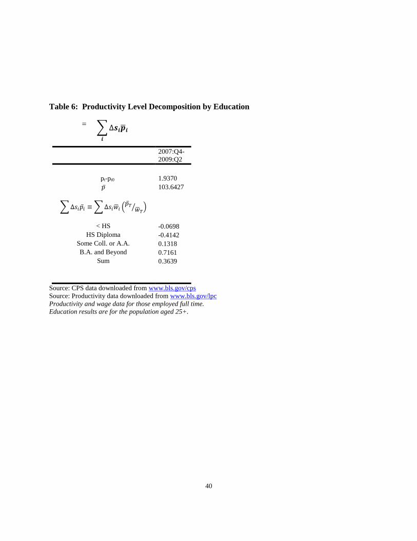
Table 6 presents the results of the decomposition. The total change in productivity over
the recession was 1.937, which was 1.87 percent of the output index. The sum of the productivity
changes induced by changes in relative shares of the educational groups equals .364, so about 19
percent of the total productivity change during the recession can be explained by composition
effects. Therefore, at the level of the economy, the conclusion is that changing shares of worker
quality groups based on education do not explain much of the gain in productivity during the
recession. Other factors, like increased effort, must account for the lion’s share of the increased
productivity.
32 Department of Labor, BLS data are used as described in Table 5.
31
V. Conclusion
Aggregate productivity has risen during recent recessions. There are two possible
explanations for increased productivity during recessions. The first is that firms lay off workers
and each employed worker is working harder. Firms make do with less because worker effort
rises during recessions when the workers’ alternatives decline. The second is that firms are
sorting workers, retaining the highly productive and letting go the least productive. By using
detailed panel data from one firm in which measures of individual worker output are available
during recession and non-recession periods, it is possible to disentangle these alternative causes
of the rise in productivity that occurred during the 2007-9 recession.
The main finding is that productivity rose in this firm because the firm made do with less.
Each worker produced more output than would have been the case during normal times: output-
per-worker rose during the recession by 5.4 percent. Labor quality changes throughout the
recession period were small despite a large amount of turnover.
Because the data are from many different establishments across the country, it is possible
to examine the effects by local labor market conditions. In those areas where the recession was
most pronounced, the productivity gains are the strongest and the increase in effort the greatest.
This same conclusion holds for non-recession years, when cross-sectional increases in
unemployment are associated with increased worker productivity.
Finally, it appears that the less productive workers are most responsive to recessions and
increases in local unemployment rates, perhaps because their alternatives diminish the most
during weak economic times.
References
32
Berger, David. 2012. “Countercyclical Restructuring and Jobless Recoveries.” Working Paper,
Yale University.
Blanchflower, David and Andrew Oswald. 2005. “The Wage Curve Reloaded.” NBER
Working Paper No. 11338.
Cameron, A. Colin, Jonah Gelbach and Douglas Miller. 2008. “Bootstrap-Based Improvements
for Inference with Clustered Errors,” Review of Economics and Statistics, 90: 414-427.
Capelli, Peter and Keith Chauvin. 1991. “An Interplant Test of the Efficiency Wage
Hypothesis,” Quarterly Journal of Economics, 106(3): 769-787.
Donald, Stephen and Kevin Lang. 2007. “Inference with Differences-in-Differences and Other
Panel Data,” Review of Economics and Statistics, 89: 221-233.
Davis, Steven J., R. Jason Faberman, and John C. Haltiwanger. Forthcoming. “The
Establishment-Level Behavior of Vacancies and Hiring.” Quarterly Journal of Economics.
Davis, Steven J. and John Haltiwanger. 1990. “Gross Job Creation and Destruction:
Microeconomic Evidence and Macroeconomic Implications.” NBER Macroeconomics Annual, 5:
123-168.
Gali, Jordi and Thijs van Rens. 2010. “The Vanishing Procyclicality of Labor Productivity.” IZA
Discussion Paper No. 5099. Institute for the Study of Labor Discussion Paper Series.
Garin, Julio, Michael Pries, and Eric Sims. 2011. “Reallocation and the Changing Nature of
Business cycle Fluctuations.” Working Paper, University of Notre Dame.
Koenders, Kathryn, and Richard Rogerson. 2005. “Organizational Dynamics Over the Business
Cycle: A View on Jobless Recoveries.” Federal Reserve Bank of St. Louis Review, 87(4): 555-
579.
Lazear, Edward P. 1986. "Salaries and Piece Rates." Journal of Business, 59(3): 405-431.
Lazear, Edward P. 2000a. “The Power of Incentives.” American Economic Review, 90(2): 410-
414.
Lazear, Edward P. 2000b. “Performance Pay and Productivity.” American Economic Review,
(90)5: 1346-1361.
Lazear, Edward P., Kathryn Shaw, and Christopher Stanton. Forthcoming. “The Value of
Bosses.” NBER Working Paper No. 18317 and Journal of Labor Economics.
33
Rebitzer, James B. 1987. “Unemployment, Long-Term Employment Relations, and Productivity
Growth.” Review of Economics and Statistics, 69(4): 627-635.
Shapiro, Carl and Joseph E. Stiglitz. 1984. “Equilibrium Unemployment as a Worker Discipline
Device.” American Economic Review 74(3): 433-444.
Shaw, Kathryn and Edward P. Lazear. 2008. “Tenure and Output.” Labor Economics, 15(4):
704-723.
Syverson, Chad. 2011. “What Determines Productivity?” Journal of Economic Literature 49(2):
326-365.
van Rens, Thijs. 2005. “Organizational Capital and Employment Fluctuations.” 2005 Meeting
Papers No. 427, Society for Economic Dynamics Meeting Papers Series.
Appendix
Additional Analysis on Compositional Changes
Please refer to the NBER working paper version for this section.
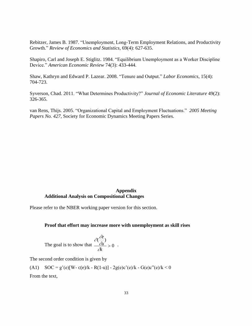
Proof that effort may increase more with unemployment as skill rises
The goal is to show that
( )e
u
k 0 .
The second order condition is given by
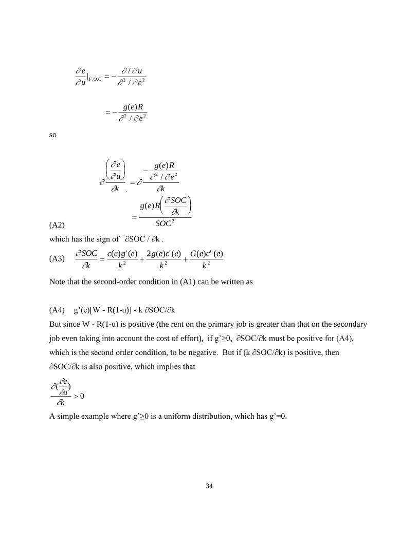
(A1) SOC = g’(e)[W- c(e)/k - R(1-u)] - 2g(e)c’(e)/k - G(e)c”(e)/k < 0
From the text,
34
e
u
u
e
g e R
e
F O C|/
/
( )
/
. . .
2 2
2 2
so
(A2)
e
u
k
g e R
e
k
g e RSOC
k
SOC
.
( )
/
( )
2 2
2
which has the sign of ∂SOC / ∂k .
(A3)
SOC
k
c e g e
k
g e c e
k
G e c e
k
( ) ' ( ) ( ) ' ( ) ( ) "( )2 2 2
2
Note that the second-order condition in (A1) can be written as
(A4) g’(e)[W - R(1-u)] - k ∂SOC/∂k
But since W - R(1-u) is positive (the rent on the primary job is greater than that on the secondary
job even taking into account the cost of effort), if g’>0, ∂SOC/∂k must be positive for (A4),
which is the second order condition, to be negative. But if (k ∂SOC/∂k) is positive, then
∂SOC/∂k is also positive, which implies that
( )e
u
k 0
A simple example where g’>0 is a uniform distribution, which has g’=0.
35
Tables and Figures
Table 1: Summary Statistics
Pre-Recession Recession and
Post-Recession
(1) (2)
Log Output Per Hour 2.21 2.33
(0.29) (0.28)
Uptime 0.96 0.96
(0.03) (0.03)
Tenure (days) 568 695
(540) (640)
State Unemployment Rate 4.55 8.05
(1.02) (2.52)
N 1,883,328 3,744,345
Notes: Means are reported with standard deviations in parentheses below.
The Pre-Recession period is June 2006 - November 2007. The data end in
May 2010. Output per hour is the average number of transactions a worker
handles in an hour, when the hour working is measured from time spent
processing transactions. Uptime is the fraction of shift time that a worker is
able to receive transactions. The mean unemployment rate at the peak of the
recession in Quarter 2 of 2009 is 9.71 percent (2.11).
36
Table 2: The Effect of the Recession on Productivity
Dependent Variable: Log (Output per Hour)
Entire Sample Balanced Sample
Establishment
Fixed Effects
Worker Fixed
Effects
Worker and Boss
Fixed Effects
Establishment
Fixed Effects
(1) (2) (3) (4)
Recession 0.054 0.054 0.053
0.048
(0.007) (0.006) (0.006) (0.004)
N 5,627,673 5,627,673 5,627,673 1,104,889
R2 0.071 0.251 0.256 0.05
Notes: The Entire Sample contains daily data from June 2006 to May 2010, for 23,580 workers. The Balanced
Sample contains only those 1,623 workers who were employed before October 2006 and who remain in the sample
as of May 2010. All specifications contain fifth order polynomials in tenure, establishment fixed effects, and 11
month fixed effects. OLS regressions contain cubic polynomials in time. Regressions with worker fixed effects
contain time squared and time cubed. Robust standard errors are clustered at the state level. Standard errors are
calculated by pairs cluster bootstrap in column (3) to deal with having both worker and boss fixed effects.

37
Table 3: Productivity Regressions with the Local Unemployment Rate
Balanced Sample
Establishment
Fixed Effects
Worker Fixed
Effects
Worker and Boss
Fixed Effects
Establishment
Fixed Effects
(1) (2) (3) (4)
Monthly unemployment rate in state 0.008 0.008 0.007 0.009
(0.003) (0.003) (0.003) (0.003)
P-value against null of 0 0.013 0.007 0.047 0.013
Impact of 5 % change in unemployment 0.039 0.041 0.037 0.044
N 5,627,673 5,627,673 5,627,673 1,104,889
R2 0.076 0.259 0.262 0.054
Entire Sample
Notes: For notes on sample composition, see Table 2. All models include a fifth-order polynomial for workers' tenure, year x
month fixed effects, and establishment fixed effects. Robust standard errors are clustered at the state level. Standard errors are
calculated by pairs cluster bootstrap using the state as the unit of analysis in column (3) with boss and worker fixed effects;
calculating the variance-covariance matrix analytically is not possible. In all cases, the p-value against the null of 0 is computed
using a t distribution (2 tailed) with G-2 degrees of freedom, where G is the number of clusters. An alternative set of calculations
uses the empirical distribution of bootstrap estimates. The distribution of bootstrap parameter values from column (3) has 1 out
of 80 draws with a value less than zero. The wild cluster bootstrap t, imposing the null hypothesis of 0, was also used to assess
the robustness of inference. The model in column (2) was estimated using data aggregated to the monthly level because of
computational considerations. The parameter estimate when using monthly aggregation was 0.0099 with a 2-tailed p-value of
0.038. Monte Carlo evidence from an experiment generating data with the exact sample size and degree of serial correlation in
the residuals from the monthly aggregated version of column (2) suggests that the wild cluster bootstrap t under-rejects in this
setting.
Dependent Variable: Log (Output per Hour)
38
Table 4: Productivity Regressions with the Local Unemployment Rate
Dependent Variables: Uptime and Quality
Establishment Fixed
EffectsWorker Fixed Effects
Worker and Boss
Fixed Effects
(1) (2) (3)
Panel A: Uptime
Monthly unemployment rate in state 0.0003 0.0004 0.0004
(0.0005) (0.0004) (0.0005)
Impact of 5 % change in unemployment
relative to mean downtime 0.038 0.051 0.051
Mean of dependent variable in pre-
recession period 0.961 0.961 0.961
N 4,863,587 4,863,587 4,863,587
R2
0.013 0.094 0.099
Panel B: Quality
Monthly unemployment rate in state 0.0196 0.0179 0.015
(0.0089) (0.0094) (0.011)
N 359,658 359,658 359,658
R2
0.775 0.79 0.793
Notes: All models include a fifth order polynomial for workers' tenure, time period (year x month) fixed effects, and
establishment fixed effects. Standard errors are clustered at the state level. In the uptime model, the impact of a 5
percent change in unemployment is calculated relative to a "downtime" baseline, where mean downtime is 1 - mean
uptime. Quality is increasing in the score, but the scale of the survey instrument changes over time; no comparison
is made relative to a mean score for the quality measures.
39
Table 5: Productivity Regressions for Stars and Laggards
Dependent Variable: Log (Output per Hour)
Establishment Fixed
Effects, Laggard
Classification Method
1
Boss Fixed Effects,
Laggard Classification
Method 1
Establishment Fixed
Effects, Laggard
Classification Method
2
Boss Fixed Effects,
Laggard Classification
Method 2
(1) (2) (3) (4)
Laggard -0.224 -0.224 -0.219 -0.218
(0.0152) -0.016 (0.015) (0.016)
0.001 0.001 0.0001 0.001
(0.004) (0.004) (0.003) (0.004)
0.011 0.011 0.011 0.011
(0.002) (0.002) (0.002) (0.002)
P-value against null of 0 on interaction term 0 0 0 0
N 1,765,499 1,765,499 1,691,163 1,691,163
R2 0.188 0.207 0.197 0.215
Monthly unemployment rate in state
Notes: The sample used to classify stars and laggards includes workers with less than 60 days of tenure and whose first day of work is prior to
November 1st, 2007. Stars and laggards are classified according to method 1 based on whether a worker's estimated fixed effect is above or below
the median of the distribution of worker fixed effects after regressing log(oph) on a fifth order polynomial in tenure, time (year x month) fixed
effects, establishment fixed effects, and worker fixed effects. The sample used to classify stars and laggards according to method 2 aggregates the
data to the weekly level and includes fewer workers because of the need for lagged data at the weekly level. Stars and laggards are classified
according to method 2 using the mean residual in levels after an Anderson-Hsiao dynamic panel regression that allows for mean reversion in
productivity. The model is a two-stage least squares regression where the first difference of log(oph) is regressed on the lagged first difference of
log(oph), first differences of the tenure polynomial, and time fixed effects. The instrument for the lagged difference is the second lag of log(oph)
in levels. The parameter estimate on the lag of log(oph) is 0.100 with standard error .015. Each of the reported second stage specifications
contains matched data from the first stage. These specifications contain a fifth order polynomial in workers' tenure, establishment, and time (year
x month dummies). Robust standard errors are clustered at the state level. The p-value is computed using a t distribution with G-2 degrees of
freedom where G is the number of clusters.
Monthly unemployment rate in state x Laggard
40
Table 6: Productivity Level Decomposition by Education
=
2007:Q4-
2009:Q2
pt-pt0 1.9370
�̅� 103.6427
∑ ∆𝑠𝑖�̅�𝑖 ≡ ∑ ∆𝑠𝑖�̅�𝑖 (�̅�𝑇
�̅�𝑇⁄ )
< HS -0.0698
HS Diploma -0.4142
Some Coll. or A.A. 0.1318
B.A. and Beyond 0.7161
Sum 0.3639
Source: CPS data downloaded from www.bls.gov/cps
Source: Productivity data downloaded from www.bls.gov/lpc
Productivity and wage data for those employed full time.
Education results are for the population aged 25+.
∑ ∆𝒔𝒊�̅�𝒊
𝒊
41
Appendix Table 1: Results from Alternative Specifications
Establishment Fixed
Effects, IV
Worker Fixed Effects,
IV
Establishment Fixed
Effects, Establishment
Time Trends
Worker Fixed Effects,
Establishment Time
Trends
(1) (2) (3) (4)
Panel A: Log (Output Per Hour)
Monthly unemployment rate in state 0.008 0.008 0.011 0.01
(0.003) (0.003) (0.004) (0.004)
N 5,627,673 5,627,673 3,063,646 3,063,646
Panel B: Uptime
Monthly unemployment rate in state 0.00028 0.00036 0.00049 0.0002
(0.00049) (0.00038) (0.00048) (0.00043)
N 4,863,587 4,863,587 2,631,021 2,631,021
Panel C: Quality
Monthly unemployment rate in state 0.022 0.004 0.017 0.011
(0.009) (0.007) (0.024) (0.024)
N 359,658 359,658 197,434 197,434
Notes: All models include a fifth order polynomial for workers' tenure, time period (year x month) fixed effects, and establishment fixed
effects. Standard errors are clustered at the state level. The IV estimates instrument for the concurrent unemployment rate in the state with the
lag of the unemployment rate in the state. The estimates in columns 3 and 4 add establishment-specific time trends. The sample in columns 3
and 4 is limited to those states with mulitple establishments.