Major Investments, Firm Financing Decisions, and Long-run Performance*

Ralf Elsas a

Mark J. Flannery b

Jon A. Garfinkel c

February 2006

Abstract

We assemble a sample of 1,558 large investments made by 1,185 firms over the period 1989-1999, and study two main issues: How do firms pay for these large investments? And how does the stock market subsequently evaluate them? We find that major investments are mostly externally financed. The pecking order and market timing effects on capital structure are transitory. Firms move toward target leverage ratios. Long-run abnormal stock returns are not generally consistent with the hypothe-sis that managers tend to overinvest with internal funds. Only firms financing large projects with (newly-raised) external funds exhibit reliably negative abnormal returns over the subsequent 1 – 3 years. JEL Classification: G14, G31, G32

Keywords: firm financing, firm investments, long-run performance

* We thank, without implicating, Jay Ritter and Mike Ryngaert for helpful comments and Stas Niko-lova for editorial assistance with the manuscript. Kasturi Rangan graciously provided our target debt estimates. This work was largely completed while Elsas was visiting the University of Florida. He gratefully acknowledges financial support from the German Research Foundation DFG under the grant EL 256/1-1. a Institute for Finance and Banking, LMU München, elsas@bwl.uni-muenchen.de. b Department of Finance, University of Florida, flannery@ufl.edu. c Department of Finance, University of Iowa, jon-garfinkel@uiowa.edu.

1. Introduction

At its most basic level, corporate finance concerns the choice of new investments and decisions about

how to finance those investments. Each of these decisions has been studied extensively, but usually in isola-

tion from the other. However, it may be inappropriate to study financing and investment decisions separately.

New investments must be financed, and the financing decision may itself affect firm value by changing inves-

tors’ expectations. The connections between capital structure and investment decisions should be most appar-

ent when a firm undertakes a large investment (Mayer and Sussman [2004]). We have assembled a sample of

such firms and study their financing decisions and their long-run stock-market performance. We screen all

Compustat firms to identify those that made “major” investments during the period 1989-1999. We separately

identify major internal or “built” investments (Compustat item #128, “capital expenditures”) and investments

“acquired” from outside the firm (Compustat item #129, “acquisitions”). We then use Compustat flow-of-

funds data to infer how these major investments were financed. We use this sample to study two questions.

First, what determines the combination of equity and debt securities issued to finance large investments? Sec-

ond, how do various combinations of investment types and financing sources affect a firm’s long-run equity

performance?

Our capital-structure results can be summarized as follows. We find that major investments are

mostly externally financed, with new debt providing at least half the required funds in the year of the invest-

ment. Only about 15 - 20% of the typical investment is financed by the sale of equity, with internal funds

supplying most of the remainder. In the event year, firm financing choices reflect some pecking order and

market timing effects, but firms systematically revise their initial financing decisions in subsequent years.

Retained earnings and new equity issues pay down debt. Ultimately, these financing decisions are consistent

with the trade-off hypothesis about capital structure: a firm’s external securities issuance reflects its position

vis-à-vis a firm-specific, target debt ratio computed from the usual combination of firm features. We also find

that financing proportions vary with firm size: smaller firms rely more on external equity funds, which seems

inconsistent with the pecking order theory of capital structure (Frank and Goyal [2003], Fama and French

2

[2003]). Finally, the data reflect a tendency for firms with higher Tobin’s Q to fund themselves by issuing

new securities.

In the long run, major investment projects are followed by significant equity under-performance.

However, financing decisions importantly affect these long-run returns. Investments funded out of the firm’s

internal resources are followed by insignificant abnormal returns, contradicting the hypothesis that managers

routinely over-invest in net operating assets. This is particularly surprising because managers are often said to

have considerable autonomy over free cash flow. In sharp contrast with the first result, we find that externally

financed investments generate significant mean underperformance over the next year. This underperformance

is greater for built investments than for acquisitions, and for any investment financed with debt(!). These re-

sults seem to challenge the conventional wisdom that debt serves as a disciplining device, or that outside

monitors are most active when a firm is issuing new securities. They also suggest a need for future research

into the differences between built and acquired investments.

The rest of this paper is organized as follows. Section 2 sets the stage for our analysis with a short lit-

erature review. Section 3 explains how we identify “major” investments, and describes the features of our re-

sulting sample firms. Financing patterns for these investments are evaluated in Section 4, and the long-run

performance results appear in Section 5. The next section reports some robustness results, and the paper con-

cludes with a summary and a discussion of the implications for other research.

2. Literature Review

Finance theory has long hypothesized that a firm’s capital structure affects its market value, although

empirical evidence remains unclear about the specifics. For example, Shaym-Sunder and Myers [1999] con-

clude that the pecking order hypothesis describes their sample of large, long-lived firms. But Frank and Goyal

[2003] show that small firms quite often issue equity, contradicting the pecking order’s assumption that man-

agers are reluctant to sell equity to relatively pessimistic outsiders. Other hypotheses about capital structure

3

focus on security mis-pricing or convergence toward a target capital structure. We consider all of these possi-

bilities when analysing how firms finance large investment projects.

Long-run equity performance studies have produced two puzzling conclusions. First, firms raising

external funds underperform otherwise comparable firms for up to five years following the financing event.

This finding applies to most types of securities.1 Although some of these conclusions do not withstand

econometric refinements (Mitchell and Stafford [2000]), the broad implication that external fund-raising gen-

erates negative stock returns provides a serious challenge to conventional concepts of market efficiency. Sec-

ond, poor stock returns follow large investments. Titman, Wei and Xie [2004] find that large increases in net

operating assets (NOA) are associated with significant underperformance, especially for firms with large in-

ternal cash flows or low leverage. 2 Lyandres, Sun and Zhang (2005) also conclude that poor performance

follows large NOA increases.

Our event firms include those making a large purchase of assets, which can be either a takeover, or

the purchase of a plant or division. Some of our results will therefore link to the extant literature on mergers

and acquisitions. Many studies conclude that the typical acquiring firm loses market value in the short term.

The literature also finds that the means of payment for an acquisition significantly affects announcement re-

turns, with equity-financed acquisitions generating more negative abnormal returns for the acquirer. However,

the evidence on acquisitions’ long-run returns is mixed. Franks, Harris, and Titman [1991] find no underper-

formance, but Loughran and Vijh [1997] and Mitchell and Stafford [2000] find that negative longer-run re-

turns are most pronounced for stock-financed acquisitions.3

1 Ritter [2003] provides a comprehensive discussion of the long-run performance effects of securities issuance. See Spi-ess and Affleck-Graves [1999] and Datta, Iskandar-Datta, and Raman [2000] on bonds; Ritter [1991] and Spiess and Affleck-Graves [1995] on equity; Hertzel et al. [2002] on private equity; Billett, Flannery, and Garfinkel [forthcoming] on bank loans. Richardson and Sloan [2003] show that the effect of securities issuance depends on how the resulting funds are deployed. 2 Titman, Wei and Xie [2004] evaluate data from 1973-1996 and identify a “takeover period” [1984-89] within which investments do not generate underperformance. Our sample (1989-99) mostly post-dates their takeover period. 3 Previous studies of firm acquisitions often use the Securities Data Corporate (SDC) database to identify acquisitions. Our list of acquisitions differs from those in two ways. First, we believe that Compustat more completely identifies the acquisition of small and/or private firms. Second, we will pick up sales of divisions or plants in addition to the acquisi-tion of entire companies.

4

Our work most closely resembles that of Mayer and Sussman [2004], who also study capital structure

changes for a sample of firms making large investments. They conclude that most large investments are ini-

tially financed by new debt, consistent with the pecking order theory of capital structure. Following the event

year, however, Mayer and Sussman [2004] find some evidence consistent with the trade-off theory, as firms

move back toward their historic debt ratios. Our study expands upon this analysis by using a SUR framework

to examine how a broader range of firm characteristics affects the financing proportions. By examining sev-

eral different financing windows, we illustrate that large investments tend to be associated with dynamic

funding patterns.4 Finally, we examine how large investments affect firm value by studying long-run per-

formance following the events. Mayer and Sussman [2004] do not investigate valuation effects.

3. Sample Selection

Our research design requires a set of “major” investment events, which reveal information about a

firm’s preferred capital structure and the market’s reaction to its investment and financing decisions. Theory

provides no clear definition of “major” investments, so we proceed with one plausible rule, that an investment

is “major” if

• it exceeds 200% of the firm’s past three years’ average investment level (its “benchmark” invest-ment), and

• the investment is at least 30% of the firm’s prior year-end total assets. 5

For each firm-year, we compute separate benchmark investment levels for built and acquired capital expendi-

tures.

4 We also distinguish between “built” capital expenditures and acquisitions, and use a different filter to identify major investments. Mayer and Sussman [2003] seek firms with large investment “spikes” – one large investment that is pre-ceded and succeeded by stable, lower investment expenditures. Examining the time series of investments associated with our major events (not reported here) suggests that the “spike” nature of Mayer and Sussman’s filter rule will iden-tify more acquisitions than built investments. 5 Analysis based on a less restrictive, alternative rule (200% of trailing investment and only 20% of total assets) yields very similar results.

5

Starting in 1974, Compustat divides “investment” into two categories: capital expenditures and acqui-

sitions. We refer to internal investment projects (pure capital expenditures) as built investments, and to exter-

nal investments as acquired investments or acquisitions. Compustat’s flow-of-funds data, which we use to

identify financing patterns, become available only in 1988. We therefore focus on investment events that oc-

curred between 1989 and 1999.6 Starting with the universe of Compustat firms also listed on CRSP, we ex-

cluded firms from the sample for any year in which:

• The firm’s book value of equity is negative in the current or the previous year.

• A firm is missing data for capital expenditures and acquisitions (items #128 and #129), or for in-come before extraordinary items (item #123, used to calculate cash-flows).

We also exclude firms from regulated industries or industries with unusual capital structures: all firms with

two-digit NAICS industry codes equal to 22 (utilities), 52 (finance and insurance), 55 (management of com-

panies and enterprises), or exceeding 90 (public administration). These screens leave 76,448 annual observa-

tions (for 11,090 firms), which we search for major investment events.

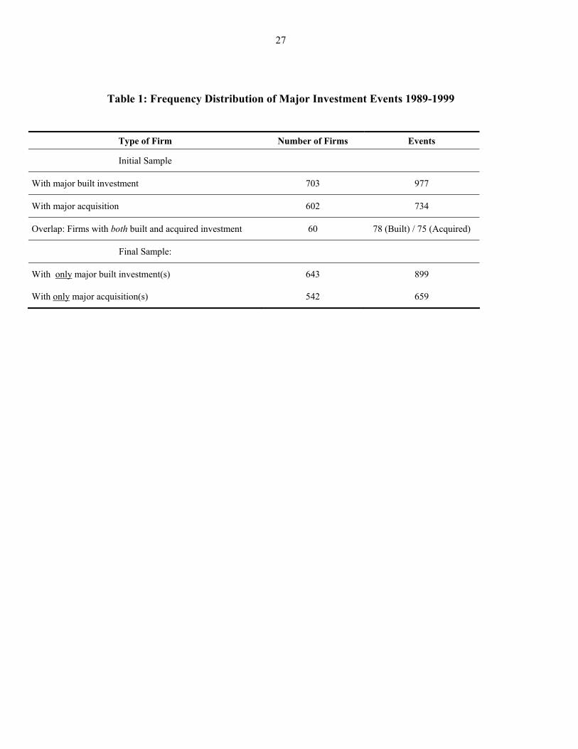
Table 1 reports the frequency distribution of the firms and events in our sample. We identify 703

firms with major built investments and 602 firms with major acquisitions. Because some firms have multiple

events, the full sample includes 977 built events and 734 acquisitions. In order to evaluate built and acquired

events separately, we omit sixty firms with both built and acquired major investments during the 1989-99

sample period. This yields 899 built events and 659 acquired events for our main testing sample.

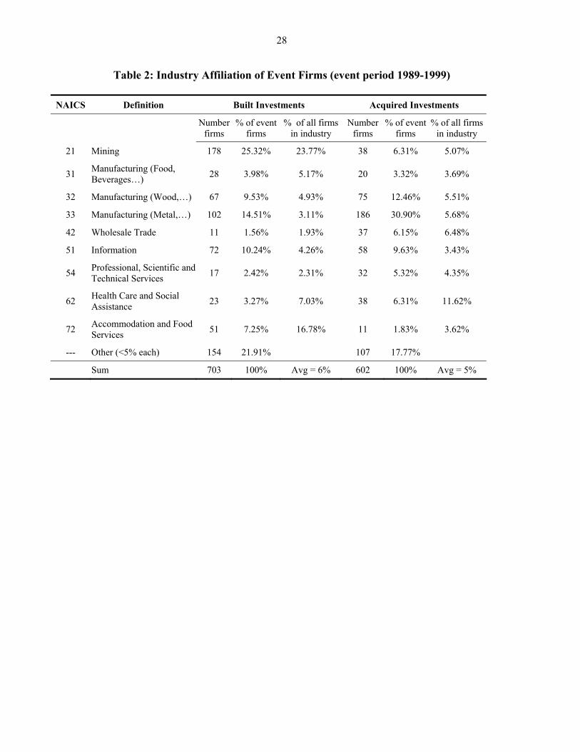
Table 2 compares our Built and Acquired sample firms to the composition of all firms on the

Compustat tape. Although some industries are more represented than others in our sample, no single industry

dominates our sample. Large investments over this time period were relatively common in the manufacturing

(NAICS = 32, 33) and Information (NAICS = 51) industries, while Health Care (62) and Accommodations

(72) undertook relatively few major investments.

6 The observation period ends in 1999 so that we can examine three full years of subsequent stock returns for all event firms. We begin identifying large investments in 1989 so that we can examine Compustat cash flow data for the year preceding investment.

6

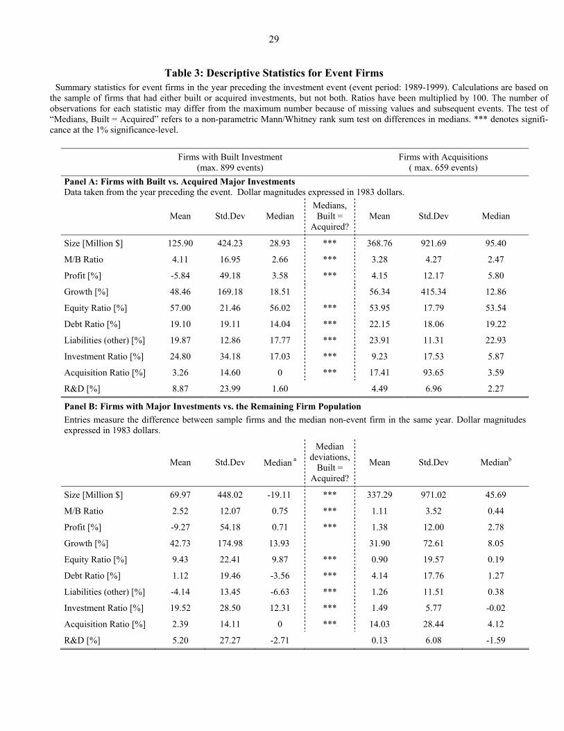
Table 3 presents descriptive statistics for the event firms. Many of the relevant variables are ratios,

which can take extreme values for a small number of observations. We therefore exclude the 0.5% highest

and 0.5% lowest observations from our reported means and medians, and we concentrate our discussion on

the median values.7 Panel A of Table 3 compares the built vs. acquiring firms’ median financial ratios for the

year preceding the investment event. These two groups differ significantly in almost all measured characteris-

tics. Most notably, the acquiring firms are far larger and more profitable than firms with built investments and

exhibit a significantly higher median debt ratio (19% versus 14%). For both groups, the median market-to-

book ratio for equity is fairly high (around 2.5), indicating that the market had been anticipating growth for

firms making major investments. The two groups’ recent asset growth rates are high, and statistically indis-

tinguishable.

Panel A of Table 3 may reflect an unavoidable element of inter-temporal comparison, since the built

and acquired investments need not occur at the same rate through time. Panel B therefore compares each

event firm to the set of non-event firms available on Compustat at the same point in time. Our sample firms

differ significantly from the non-event populations in nearly every dimension. Firms with large Built invest-

ments tend to be smaller, less levered, faster-growing, and less R&D-intensive than the non-event firms in

Compustat. Acquiring firms tend to be larger, faster-growing and slightly less R&D-intensive. The rank sum

test results in the middle column of Panel B indicate that the cross-sectional differences between firms with

built investments and acquisitions resemble those in Panel A.

4. Capital Structure (Financing) Decisions

We have identified firms that are very likely to be raising external funds. The literature on capital

structure provides a multitude of factors that might influence their financing choice. Our data can indicate the

7 The sample is truncated only when reporting the statistics in Table 3. We use all observations when identifying event firms and conducting tests of financing and long-run performance.

7

extent to which sample firms’ behaviour is consistent with the pecking order hypothesis, the trade-off hy-

pothesis, and the market-timing hypothesis.

The Appendix describes how we aggregate Compustat’s annual cash-flow data into four main financ-

ing sources. The following identity must hold for each firm over an arbitrary time interval:

Invest i = Equityi + Debti + Internali + Otheri (1)

where Invest i is the sum of firm i’s Built and Acquired capital expenditures during the interval

Equityi is the dollar value of (net) common and preferred share sales during the interval (Compustat items 108 + 115). Debt i is the net change in long-term and short term debt during the interval (Compustat items 111 plus 114 less 301). Internal i is operating cash-flows, defined as after-tax income before extraordinary items plus depre-ciation and amortization less cash dividends (Compustat items 123 + 125 - 127). Otheri is the aggregate of all other funds flow categories, including changes in working capital, asset sales, and statistical discrepancies.

Although (1) must hold within each accounting period, some of the funds required for a large investment

might have been raised in prior years. If a firm issued debt or equity in year τ-1, the event-year cash flows

might not reflect how the financing truly occurred (Mayer and Sussman [2004]). For example, suppose a firm

issues equity shares in τ = -1 and temporarily uses the funds to pay down a bank line of credit, which is then

drawn to purchase new assets.8 The event-year values in (1) would indicate a Debt-financed investment. If

we examine changes over the [-1, 0] window, however, we correctly observe that the investment was Equity

financed. (The debt increase in τ=0 exactly offsets the debt reduction in τ=-1.) Likewise, a firm’s subsequent

financing decisions could either reinforce or offset the leverage effect of the event-year's financing. By exam-

ining financing sources over several event windows, we can identify any systematic effects of this sort.

4.1. Financing Decisions: Univariate Results

8 Sufi [2005] indicates that bank lines are often used to adjust leverage.

8

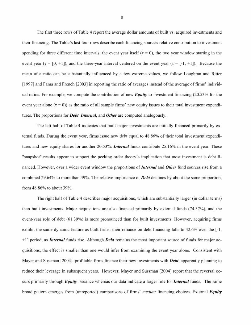
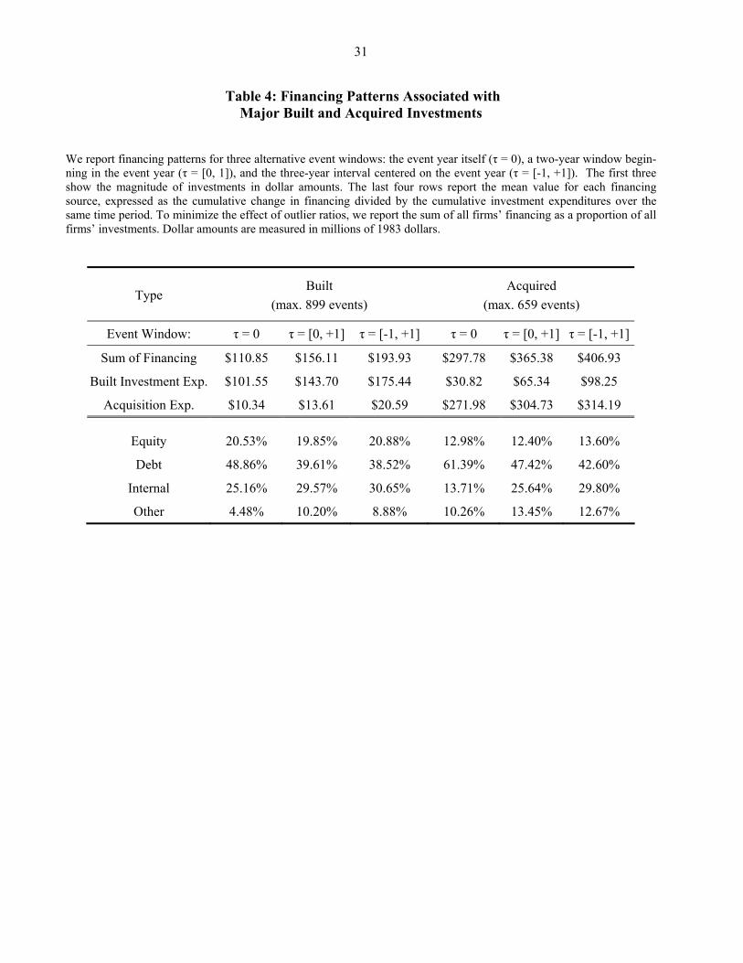
The first three rows of Table 4 report the average dollar amounts of built vs. acquired investments and

their financing. The Table’s last four rows describe each financing source's relative contribution to investment

spending for three different time intervals: the event year itself (τ = 0), the two year window starting in the

event year (τ = [0, +1]), and the three-year interval centered on the event year (τ = [-1, +1]). Because the

mean of a ratio can be substantially influenced by a few extreme values, we follow Loughran and Ritter

[1997] and Fama and French [2003] in reporting the ratio of averages instead of the average of firms’ individ-

ual ratios. For example, we compute the contribution of new Equity to investment financing (20.53% for the

event year alone (τ = 0)) as the ratio of all sample firms’ new equity issues to their total investment expendi-

tures. The proportions for Debt, Internal, and Other are computed analogously.

The left half of Table 4 indicates that built major investments are initially financed primarily by ex-

ternal funds. During the event year, firms issue new debt equal to 48.86% of their total investment expendi-

tures and new equity shares for another 20.53%. Internal funds contribute 25.16% in the event year. These

"snapshot" results appear to support the pecking order theory’s implication that most investment is debt fi-

nanced. However, over a wider event window the proportions of Internal and Other fund sources rise from a

combined 29.64% to more than 39%. The relative importance of Debt declines by about the same proportion,

from 48.86% to about 39%.

The right half of Table 4 describes major acquisitions, which are substantially larger (in dollar terms)

than built investments. Major acquisitions are also financed primarily by external funds (74.37%), and the

event-year role of debt (61.39%) is more pronounced than for built investments. However, acquiring firms

exhibit the same dynamic feature as built firms: their reliance on debt financing falls to 42.6% over the [-1,

+1] period, as Internal funds rise. Although Debt remains the most important source of funds for major ac-

quisitions, the effect is smaller than one would infer from examining the event year alone. Consistent with

Mayer and Sussman [2004], profitable firms finance their new investments with Debt, apparently planning to

reduce their leverage in subsequent years. However, Mayer and Sussman [2004] report that the reversal oc-

curs primarily through Equity issuance whereas our data indicate a larger role for Internal funds. The same

broad pattern emerges from (unreported) comparisons of firms’ median financing choices. External Equity

9

plays a small role in funding major investments, particularly for acquisitions. Debt is the most important sin-

gle source of new funds, and the majority of Debt is issued in the event year. Over time, Internal funds dis-

place Debt.

The ratios of averages reported in Table 4 mitigate the impact of a few extreme ratios on the reported

balance sheet contributions. However, those ratios cannot be compared via simple statistical tests. We next

examine how firm size affects median funding decisions, which are readily compared across groups by means

of a non-parametric Mann/Whitney rank sum test. Mann/Whitney rank sum tests indicate that our acquiring

firms use more Debt and less Equity than firms with built investments, particularly in the event year

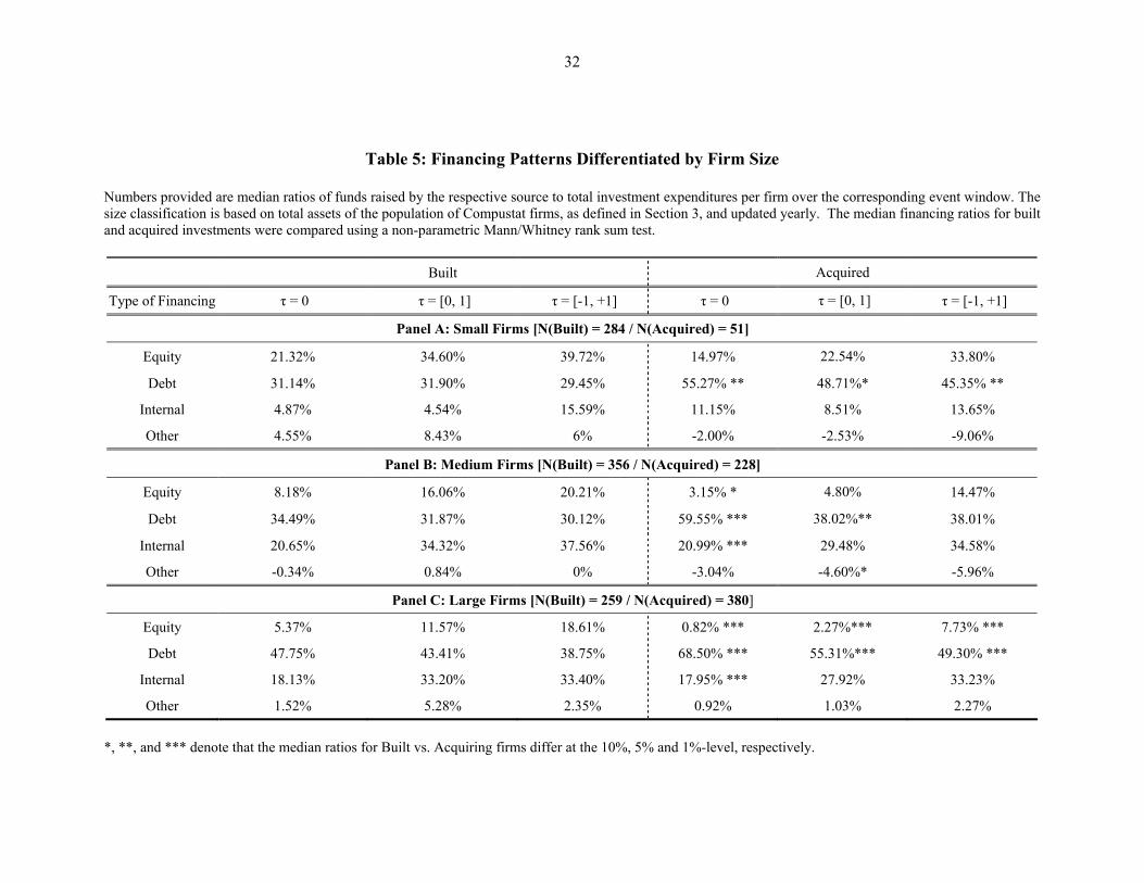
Previous writers have found that securities issuance activities vary substantially with firm size. Table

5 reports median financing ratios for each size group over three event periods. The results clearly indicate

that firm size matters. For example, over the broadest [-1, +1] window, Debt provides the plurality of funds

for Large Firms and for all acquisitions. Medium Firms finance the largest proportion of their Built invest-

ments with Internal funds (38%), while Small Firms’ greatest financing source is Equity (40%). The extent

to which financing choices differ with firm size is further illustrated in Figure 1. For each fiscal year, we sort

the universe of Compustat firms that were searched for major investments into three equal-sized groups on the

basis of their book assets. Our event firms are then placed into the “Small”, “Medium”, or “Large” grouping.9

Figure 1 plots median financing patterns during the event year (τ = 0) for different-sized firms. Debt provides

the largest proportion of investment funds for both investment types and for all firm size groups. Debt is more

important for larger firms, and when financing acquisitions.10

Table 5 again indicates that financing patterns change as we widen the event window. Over time,

firms replace some of the Debt issued in year 0 with Internal funds and new Equity. Internal funds grow

more rapidly at larger firms and external Equity grows more rapidly at smaller firms.

9 The results are qualitatively similar when we form size groupings on the basis of equity market value instead of book assets. 10 Equity is more important for funding smaller firms, as shown by Frank and Goyal [2003].

10

4.2. Financing Decisions: Seemingly Unrelated Regression Results

The univariate analysis in Tables 4 and 5 appears broadly consistent with the pecking order hypothe-

sis. Debt finances the largest part of major investments in the event year, but firms tend to offset some of the

leverage effect soon afterwards. The key question about capital structure is not whether Debt initially funds

new investments, but whether that choice has a persistent effect on a firm’s capital structure. In addition, fi-

nancial decisions for these large investments may reflect a firm’s position vis-à-vis some type of target lever-

age ratio.

We now investigate multiple determinants of financing behavior via the regression

Fiτ = α + β1 DEV-1 + β2 Profit-1 + β3 ln(Size-1) + (2)

β4 INV_TA-1 + β5 FA_TA-1 +β6 Runup-17,-6 + β7 Q-1 + εiτ where

Fiτ = the proportion of the net new investment financed by one of the four funding sources: i = Eq-uity, Debt, Internal, and Other) during the event window τ. DEV = the deviation from target leverage: the firm’s estimated target debt ratio (from Flannery and Rangan [forthcoming]) less its actual market debt ratio at t = -1. Profit = net annual income as a proportion of yearend total assets

ln(Size-1) = log of the firm's yearend book assets. Table 5 indicates a substantial effect of size on fi-nancing choices.

INV_TA = the ratio of investments (built plus acquired) during the event window to book total assets at the yearend preceding the event window. Larger investments may be financed differently. FA_TA = the firm's yearend book value of fixed assets as a proportion of total assets; a measure of “debt capacity”. Runup = the stock's excess return, relative to the market, over the months [-17,-6] if the event win-dow starts in τ=0 and over the months [-29,-18] if the event window starts in τ=-1. Firms tend to issue stock following a Runup in the price (Korajczyk, Lucas and MacDonald [1991]). Q = the ratio of the firm's market value (market value of equity plus book value of debt) to the book value of assets at the yearend preceding the event window. Q measures the firm’s investment oppor-tunity set.

We specify a regression of the form (2) for each of the four funding sources and estimate them as seemingly

unrelated regressions, constraining each independent variable's coefficients to sum to zero across the four

11

equations. This constraint requires that a change in firm characteristics will shift its reliance on alternative

funding sources, but the net effect on all funding decisions must leave the investment fully funded. 11

The firm's deviation from target leverage (DEV) bears particular discussion. Following Flannery and

Rangan [forthcoming], we define leverage as

tititi

titi PSD

DMDR

,,,

,, += , (3)

where Di,t denotes the book value of firm i’s interest-bearing debt (the sum of Compustat items 9 plus 34) at

time t, Si,t denotes the number of common shares outstanding (Compustat item 199) at time t, and Pi,t denotes

the price per share (Compustat item 25) at time t. Flannery and Rangan [forthcoming] fit a partial-adjustment

model to the set of all industrial firms:

MDRi,t+1 – MDRi, t = λ (MDRi,t+1* - MDRi,t) + 1,~

+tiδ (4)

= λ (DEVit) + 1,~

+tiδ

According to this specification, the typical firm annually closes a proportion λ of the deviation (“DEV”) be-

tween its actual (MDRt) and its desired leverage (MDRt+1*). Specifying the desired (target) leverage as a lin-

ear combination of firm characteristics gives the estimable model

MDRi, t+1 = (λ β) Xi,t + (1-λ) MDR i,t + 1,~

+tiδ . (5)

Where X is a vector of variables commonly used to proxy for a firm's target debt ratio and β is a coefficient

vector.12

11 Since it is an accounting identity, all investment expenditures need to be financed. The slope coefficients measure relative importance of regressors across each type of financing (the system of equations). These coefficients need to add up to zero to let the accounting identity hold. The financing types’ fractions are reflected in the intercept terms. We also estimated a SUR model that constrained the four intercept terms to sum to unity, with very similar results to those pre-sented in Table 6. 12 Relevant firm characteristics include earnings per asset dollar, the assets' market to book ratio, depreciation expense as a proportion of total assets, the log of (real) total assets, fixed assets as a proportion of total assets, R&D expenditures as a proportion of total assets, the firm's industry median MDR value, and a dummy variable indicating whether the firm has a credit rating. Flannery and Rangan [forthcoming] also include firm fixed effects, which have important implica-tions for their estimated adjustment speeds (λ). We thank Kasturi Rangan for computing the estimated target values.

12

We use the estimated coefficients (λ, β in (5)) from Flannery and Rangan's "base model" (their Table

2, column 7) to estimate a target debt ratio for each firm at the start of each year. The trade-off theory of capi-

tal structure implies that the Debt proportion should be positively related to DEV. A firm with DEV < 0 is

"over leveraged" and should be seeking to reduce its leverage by issuing equity; a firm with DEV > 0 should

be trying to increase its actual leverage. Merging these target debt ratios with the other data on investing firms

leaves 529 Built large investments and 498 Acquired large investments.

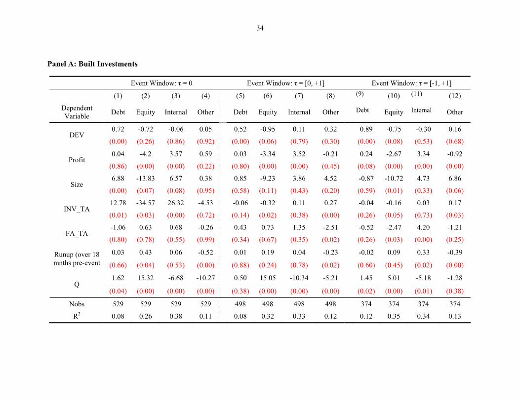
The results of estimating (2) for the [0], [0,+1], and [-1,+1] event windows are presented in Table 6.

Consider first the event-year (τ = 0) results for Built investments in Panel A, columns 1 - 4. The first row of

coefficients indicates that DEViation from the firm's target debt ratio has a significantly positive effect on

Debt and a similar-sized (but insignificant) negative effect on Equity. These coefficients imply that firms fi-

nance their large investments in a way that moves them toward a target leverage ratio. The leverage DEVia-

tion has smaller, insignificant effects on the proportion of investment financed with Internal and Other funds.

Higher (lagged) profitability has no direct effect on Debt, but clearly results in a substitution of Internal fi-

nancing for external Equity. This implies that profitability does not influence the marginal Built investment’s

effect on firm leverage. Larger firms (as measured by Size) show a strong inclination to finance with Debt

and Internal funds over Equity. Larger investments (INV_TA) tend to be financed with more Debt, and less

external Equity. We also find that firms with more fixed assets ("debt capacity") have no marginal preference

among financing sources, but perhaps this effect is fully captured in the target debt ratio. The last two rows in

Table 6 present evidence that market timing influences financing decisions in the event year. Runup has a

significantly positive effect on Equity, while a higher Tobin’s Q increases the use of both types of external

funds while substantially discouraging use of Internal and Other sources.

Over the short run (τ = 0), this evidence is consistent with both the pecking order hypothesis (Debt

predominance) and trade-off theory (DEV results). Firms also appear to pay some attention to market timing

(Runup results) in their financing decisions. These conclusions contrast somewhat with Mayer and Sussman

[2004], who only provide support for the trade-off theory in the long-run.

13

Columns 5-8 of Panel A employ a wider event window, from the start of the event year through the

end of the following year (τ = [0,1]). The dependent variable sums the new financing obtained from each

source over the two years, deflated by the amount of two-year investment volume. The leverage targeting

effect remains strong: DEV has a significantly positive effect on Debt and significantly (p = 6%) negative

effect on Equity. The negative (positive) effects of profitability on Equity (Internal) also persist over the

longer time frame. The tendency of larger firms (“Size”) to rely on Debt instead of Equity in the event year is

somewhat attenuated and no longer statistically significant. INV_TA has smaller, less significant effects on

financing choices, and FA_TA’s effect remains insignificant. Turning to the market timing variables in the

last two rows of Panel A, we find that the impacts of Runup are much smaller over the wider window, and no

longer statistically significant. The preference for Equity finance manifested in the event year reverses sign in

year τ = 1, and becomes insignificant. This manifestation of a “market timing” effect only affects leverage

temporarily. A high Q continues to encourage Equity finance, consistent with the hypothesis that growth

firms prefer lower leverage, but the effect on Debt has lost its statistical significance.

Comparing the results for τ=0 and the longer event window from [0, +1] makes clear the importance

of viewing a firm's financing decisions over an [appropriately lengthy] adjustment period. Some of the event

year effects are reversed, with important implications for the theory of capital structure, like the temporary

effect(s) of market timing. We widen the window even further in columns 9-12 of Table 6’s Panel A, which

reports SUR estimates over the event window [-1, +1]. We include the pre-event year to allow financing of

major investments before the actual undertaking of the investment.13 The results are mostly unchanged. De-

viations from the target debt ratio (DEV) systematically drive equity and debt issues. Greater profitability

causes a firm to replace Equity with Internal financing. As with the [0, 1] window, the stock price runup car-

ries an insignificant coefficient, consistent with Runup having only a transitory effect on financing decisions.

13 Widening the event window creates a few situations in which a firm has major investment events in adjacent years, which we then treat as a single event. We omit events that include another large investment in either the preceding or subsequent year.

14

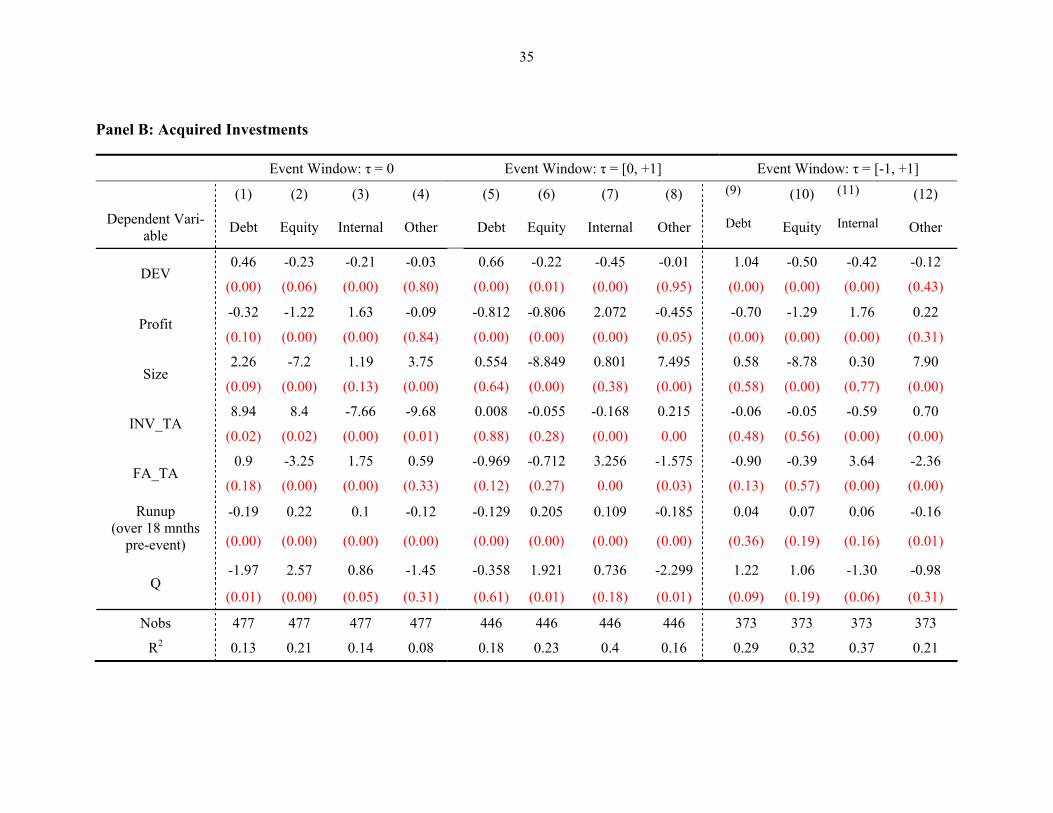
The results for large Acquisitions, in Panel B of Table 6, are quite similar. Most importantly, the coef-

ficients on DEV clearly reflect efforts to move a firm toward its target leverage ratio. However, one difference

is that the share price Runup persistently encourages Equity and Internal funds use while discouraging use of

Debt, even over the longer event window [0,+1]. The former makes intuitive sense. Firms have an incentive

to issue equity after a stock price Runup, but this effect vanishes when the pre-event year is included in the

“financing period.”

Before turning to the long-run performance issues, we summarize the observed financing patterns for

major investments. First, and most important, we provide evidence that firms systematically adjust capital

structures towards a target debt ratio (even) in the case of major investments. Market-timing and pecking or-

der effects appear only as transitory effects in the data. Second, the financing mix changes in important ways

after the event year. Hence, empirical studies of capital structure should incorporate a time dimension – the

time interval after which they assume that the firm has completed its financing decisions for a specific in-

vestment.14

5. Long-Run Equity Returns

We now investigate the valuation effects of major investments. We estimate these effects using long-

run performance methods for two reasons. First and foremost, not all large investments are announced, ren-

dering event study approaches meaningless. Second, financial market frictions (e.g. short sale constraints)

may temporarily bias price responses to some announced investments. We study how financing and invest-

ment decisions interact because many authors have previously shown that poor performance follows securities

issuances. With most investments funded from multiple sources, however, categorizing financing decisions

14 For example, Hovakimian, Hovakimian and Tehranian [2004] argue that firms undertaking a recapitalization should be near their target leverage ratios, but the same is not necessarily true for other firms.

15

becomes problematic. We concentrate on investments associated with two sorts of financing “predomi-

nance”: Internal vs. External and (among the latter firms) Debt vs. Equity. 15

• Internal: An investment is predominantly internally funded if Internal funds finance at least 50% of investment expenditures, while Debt, Equity, and Other sources each contribute less than 50%.16

• External: An investment is predominantly externally funded if Debt and Equity together contribute at

least 50% of investment expenditures, and Internal and Other sources each contribute less than 50%.

Out of 899 Built events, we categorize 149 as Internal, 434 as External, and (by subtraction) 316 were

funded with a relatively balanced mix of Internal and External funds. Out of 659 Acquired events, we cate-

gorize 53 as Internal, 429 as External, and 177 as lacking a predominant financing source.

Among the External cases, we further identify predominant financing as

• Equity: An investment is predominantly Equity funded if at least 50% of investment expenditures come from new equity issuance, while Debt, Internal and Other financing each contributes less than 50%.

• Debt: An investment is predominantly Debt funded if at least 50% of investment expenditures come

from new debt issuances, while Equity, Internal and Other financing each contributes less than 50%. Among the 434 Built investments with predominantly External funding, this procedure yields 113 predomi-

nantly Equity and 209 predominantly Debt events. By subtraction, therefore, 112 firms had no dominant

source of external funds. Out of 429 External Acquired events, 66 were predominantly Equity, 293 were

predominantly Debt, and only 70 had no predominant funding source.

Note that many major investments are funded with a relatively diffuse mixture of Internal, Debt, Eq-

uity, and Other funds. These projects cannot be characterized as predominantly funded with “debt” vs. “eq-

uity,” or by “retained earnings” vs. “external funds.” At least for these large investments, we find little evi-

dence to support the “pecking order” implication that firms fund their investments primarily using Internal

funds. Our sample’s financing decisions seem more complex than many textbook descriptions imply.

15 We have shown above that financing proportions change in systematic ways as the event window widens. The num-bers in the text and in Tables 7-8 describe the sample when “predominant” financing is based on the τ = [0, 1] window. Panel B of Table 9 reports long-run performance for financing groups identified for the τ = 0 window. Unreported re-sults based on the widest (τ = [-1, +1]) event window are also very similar. 16 This condition on Debt, Equity and Other funding sources rules out the possibility that refinancing transactions (e.g. issuing equity to retire debt) cause more than one type of funds to “provide” a majority of required amount.

16

5.1. Measuring Long-Run Performance

Lyon, Barber, and Tsai [1999, p. 198] observe that “the analysis of long-run abnormal returns is

treacherous.” An extensive literature evaluates alternative methodologies for measuring the long-run perform-

ance of stocks (e.g., Barber and Lyon [1997], Kothari and Warner [1997], Lyon, Barber, and Tsai [1999],

Mitchell and Stafford [2000]). Obstacles to computing meaningful statistics include the skewness of abnormal

return distributions, the characteristics of benchmark or peer groups, and cross-sectional correlation of events.

The potential cross-sectional correlation problem might be particularly important when analyzing firm in-

vestments because aggregate investment varies over the business cycle. Table 2 also indicates that major in-

vestments tend to cluster in specific industries. We will utilize three distinct methodologies to ensure that our

results are robust.

Our first two measurement techniques accommodate cross-sectional correlations by evaluating the re-

turns to portfolios of firms that had an event sometime in the preceding 12 months (Mitchell and Stafford

[2000]).17 The calendar-time portfolio approach is based on the Fama and French [1993] three-factor model.

Each month, we form a portfolio of all firms with an event within the prior 12 months, and regress the portfo-

lio’s time-series excess return on the three Fama and French [1993] factors:

tptptptftmpptftp HMLhSMBsrrrr ,,,,, )( εβα +++−+=− (6)

where rp,t denotes a portfolio return at time t,

rf,t is the risk-free interest rate,

rm,t is the return of the market portfolio

SMBt is the zero-investment portfolio representing the return difference between a portfolio of small and large stocks, HMLt is the return difference between a portfolio of high book-to-market and low book-to-market stocks.

17 Our 12-month performance measures are presented for the sake of comparison with Titman, Wei and Xie [2004]. We also present results for a 36-month horizon.

17

A negative intercept (αp) indicates under-performance. 18

Our second method compares the event firms to peers, allowing us to avoid the restriction in (6) that

the factor loadings remain constant over the entire estimation period. Vijh’s [1999] calendar-time abnormal

returns (CTAR) approach requires that we first calculate the monthly return to the portfolio of firms that had

an event within the last 12 months. We then subtract the monthly return on a portfolio of peer firms to obtain

monthly excess returns. We calculate a t-statistic for the average of these monthly excess returns using the

time series standard deviation of monthly excess returns. The results reported in the text describe peer firms

selected on the basis of their equity market value and book-to-market ratio, as in Spiess and Affleck-Graves

[1999].19 As a robustness check, we repeated the CTAR analysis for peer firms based on calendar time, size,

book-to-market, and industry affiliation, with similar results.

Our third approach to measuring long-run performance follows Titman, Wei and Xie [2004] in apply-

ing the methodology of Daniel, Grinblatt, Titman and Wermers (“DGTW”) [1997]. Each year, we sort all

traded stocks into five equity market size groups, each of which is then sorted into five book-to-market

groups, each of which is then sorted into five momentum groups.20 This process yields 125 portfolios. Each

event firm’s return is then compared to that of the appropriate benchmark portfolio. The time-series standard

deviation of excess returns is then used to assess whether the mean excess return differs statistically from

zero.

Tables 7 and 8 present abnormal return estimates for portfolios of firms with various financing deci-

sions for built and for acquired major investments. We initially apply all three estimation methods to the 12-

18 This interpretation of αP assumes that the Fama/French three-factor model is properly specified, but some evidence suggests that the model describes small firms relatively poorly. Mitchell and Stafford [2000] suggest making inferences from a bootstrap distribution. We estimate the model for 1,000 sets of peer firms selected to resemble the event firms in calendar time, size and book-to-market. The observed distribution of the intercept term (αP in (6)) captures “normal” variation in the model’s intercept, which can be used to evaluate the statistical significance of our event firms’ αP esti-mates. These adjustments did not qualitatively affect the long-run performance results produced by our Fama/French measure. 19 We require a close size match (+/- 10%) because Barber and Lyon [1997] find this dimension to be particularly im-portant for larger event firms. 20 Book equity is based on common equity. Market equity is the fiscal year-end market capitalization. Size is measured as a firm’s market capitalization at the beginning of the month.

18

month period starting in the first month of the fiscal year after the event. We subsequently provide some 36-

month estimation results in Table 9. In all cases, we seek evidence whether internal and external financing

impose different constraints on a manager’s ability to invest. (These results relate to the disciplining effects of

debt financing and the market for corporate control.) We are also interested in comparing the long-run per-

formance effects of built vs. acquired investments.

5.2. Results

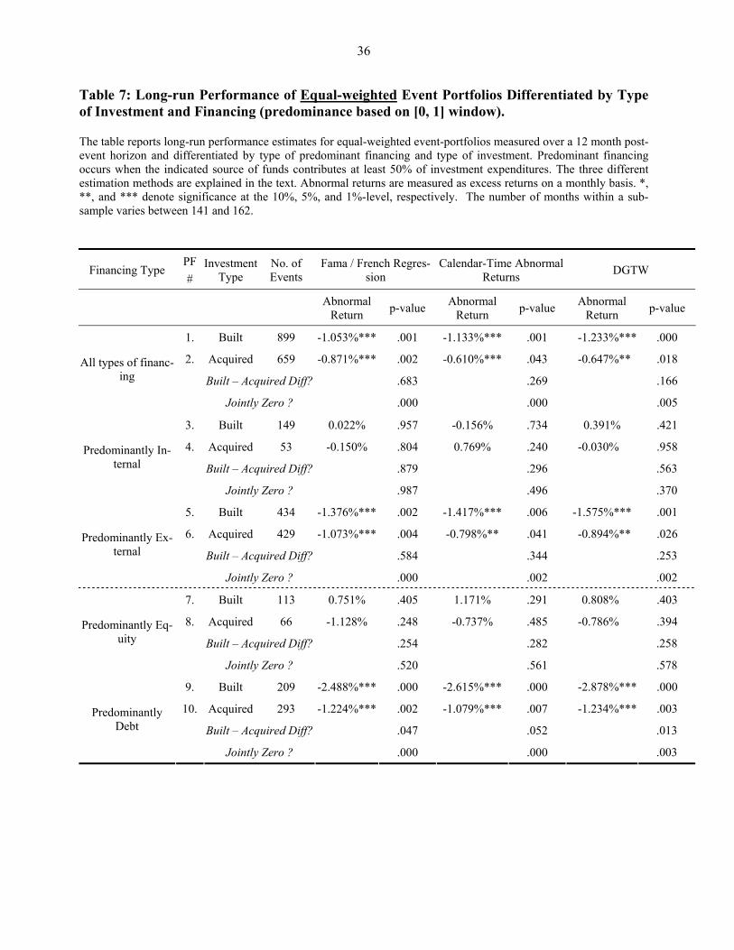
We initially categorize the predominant type of financing using the τ = [0,1] window. Table 7 pre-

sents abnormal return calculations for equal-weighted portfolios of event firms. The first two portfolios show

significant under-performance (7% - 12%) in the year following the event year, consistent with the findings of

Titman, Wei and Xie [2004] that larger investments lead to poor performance. However, we find that all in-

vestments are not alike. Internally-funded projects (portfolios 3 and 4 of Table 7) have relatively small ab-

normal returns, which do not differ significantly from zero. In sharp contrast, the externally-financed projects

(portfolios 5 and 6) have large and reliably negative abnormal returns. When we further divide the externally-

financed sample into those that are predominantly equity vs. predominantly debt (portfolios 7 – 10), we see

that significant under-performance is associated only with debt-financed projects.21 The debt-funded, Built

projects are particularly bad for shareholders. By all three measurement methods, these investments elicit

significantly more negative abnormal returns than the Acquired projects (p < .05).

Researchers often detect significant long-run underperformance in equal-weighted event portfolios,

only to have these effects disappear with value-weighting. Table 8 shows that value-weighting leaves most of

the significant effects in Table 7 unaffected. The value-weighted mean abnormal returns provide less support

for the hypothesis that large investments are always bad for shareholders. However, support for underperfor-

mance following externally-financed projects remains strong, and the debt-financed projects are (again)

largely responsible. Unlike the equal-weighted results in Table 7, value weighting provides some support for

21 In fact, Built projects funded predominantly with Equity have positive, but insignificant, mean abnormal returns.

19

the hypothesis that equity-funded acquisitions harm investors in the long run, perhaps because larger firms are

more likely to make major acquisitions with equity. The value-weighted results do not reject the hypothesis

that internally-funded projects give rise to no abnormal returns.

Table 9 demonstrates that the implications of Tables 7 and 8 are robust to longer performance inter-

vals (36 months as well as 12) and to a shorter event window (predominance defined on the basis of τ = [0]

rather than τ = [0, 1]). Panel A is based on the [0, 1] definition of predominance and the left half therefore

repeats (qualitatively) some of the information provided in Tables 7 and 8. The first two rows of Panel A

show that Built or Acquired investments are more likely to generate significantly negative abnormal returns

under equal-weighting than under value weighting. As pointed out by Loughran and Ritter [2000], this most

likely reflects the greater difficulty of shorting small stocks, which can therefore remain mispriced for longer

periods of time. The next broad conclusion from Panel A of Table 9 is that internally financed projects

never(!) generate significant underperformance. In contrast, all categories of externally-financed, Built in-

vestments and most externally-finance Acquisitions elicit negative mean abnormal returns. The last two rows

of Panel A provide strong support for the hypothesis that Debt-financed, Built projects are followed by sig-

nificant underperformance. The evidence is, again, more mixed for Debt-financed acquisitions or for any type

of Equity-financed projects.

Panel B of Table 9 repeats the analysis with predominance defined on the basis of only the event

year’s financing (τ = 0). The main results are identical: Internally-funded projects never lead to statistically

significant abnormal performance; Built investments do, especially when they are Debt-funded.

5.3. Interpretation

Tables 7 – 9 indicate that financing (debt vs. equity) and investment (built vs. acquired) choices have

important interaction effects that influence firm value. We believe we are the first to illustrate this point.

More specifically, we reach three main conclusions about long-run performance.

First, it appears that large investments per se do not generate poor performance, since predominantly

internally financed investments exhibit insignificant ex-post returns. Like Titman, Wei, and Xie [2004], we

20

conclude that large investment outlays are followed by poor stock returns. However, our results differ from

those of Titman et al. because significant underperformance is associated only with external financing, par-

ticularly debt financing. This suggests that external financial claimants do not impose the discipline hypothe-

sized in the extant literature on capital acquisition (Easterbrook [1984]). The specific disciplining effects of

debt (Jensen [1986]) also fail to appear in our sample.

The inverse of this first conclusion is that internally-funded projects engender no long-run underper-

formance. These are large projects, for which the firm may have accumulated non-trivial amounts of cash in

advance of the investment. Agency costs are sometimes hypothesized to be extreme in such situations. Nev-

ertheless, the managers in our sample make reasonable investment decisions with internal funds, in an envi-

ronment with relatively little external scrutiny. By contrast, one generally assumes that outside monitors are

most active when new securities are being issued. In our results, however, the investments financed with ex-

ternal funds are least likely to perform well. This poses a serious challenge to some current assessments of

principal-agent problems within U.S. firms.

Finally, our finding that Built investments under-perform Acquired investments is consistent with

disciplining effects of the market for corporate control (Jensen [1986]). Perhaps shareholders must approve

large acquisitions, while Built investments do not receive such explicit scrutiny.

6. Robustness

In addition to the results reported in Tables 6 - 9, we conducted a series of robustness tests with re-

spect to applied sample selection and methodology. All of these exercises yielded qualitatively the same re-

sults as those reported in the previous sections.

Identifying the Event Firms. Our definition of “major” firm investments is essentially arbitrary. For

the results reported above, we selected firms whose absolute capital/acquisition expenditures exceed 200% of

a trailing (3-year) average investment ratio and 30% of the prior year’s total assets. We replicated our long-

run performance analysis with a sample in which “major” investments exceeded only 20% of the firm’s prior

21

year-end assets. The main conclusions are unchanged. Externally-financed investments produce significant

under-performance but internally-financed investments do not. The results are, again, somewhat more sig-

nificant under equal-weighting than under value-weighting.

IPO Dominance? Ritter [1991] has shown that the mean firm underperforms the market in the three

years following its IPO. Since new, small firms might also tend to make relatively large investments, perhaps

our long-run performance results reflect primarily the tendency of new firms to underperform. We find that

about 20% of our major investment events occurred within three years of the firm’s IPO. 22 Omitting these

recent IPO events from our sample yields similar conclusions about long-run performance. In other words,

new firms do not appear to drive our earlier results.

Book-valued Target Leverage Estimates. The DEViation variable in Table 6 assumes that firms tar-

get market-valued leverage ratios. However, some researchers prefer to measure leverage in book terms and

many researchers report results for both book and market measures. When we define define leverage in book-

value terms (the book value of interest-paying debt over total book assets), DEV becomes the difference be-

tween actual and target book leverage. The results are very similar to those reported in Table 6.

Errors-in-Variables. The DEV variable in Table 6 is a generated regressor, which may bias our SUR

estimates unless the measurement errors are uncorrelated with the regression residuals.23 We therefore con-

duct three robustness checks. First, we estimate the same set of regressions separately as 2SLS, where DEV

is treated as an endogenous variable (we use lagged DEV as the instrument). Second, we estimate simple OLS

(with and without imposing the constraint that coefficients add-up to zero). Finally, we employ a bootstrap

procedure to both OLS and 2SLS to estimate the true distribution of coefficient errors. None of these ap-

proaches reverses the main conclusions in Table 6. We also checked the sensitivity of these results to winso-

rizing the data – again with no substantive change.

22 We thank Jay Ritter for providing access to his IPO database. 23 Other researchers have also ignored this potential source of estimation error (e.g., Hovakimian, Opler and Titman [2001], Fama and French [2002]).

22

7. Summary and Conclusions

This paper studies U.S. firms that made relatively large capital expenditures or acquisitions during the

1989-99 period. Such activities are necessarily accompanied by major financing decisions. Because these in-

vestments represent a substantial proportion of our sample firms’ total assets (at least 30%, by construction),

we anticipate that the associated financing decisions will reflect managerial attitudes toward overall capital

structure.

We find similar financing patterns for both built and acquired major investments. Debt issues pay for

the largest proportion of new investments in the event year, particularly for large firms. Equity has a relatively

small role. This initial pattern seems consistent with a pecking order view of capital structure. Over time,

however, firms systematically replace the new debt with equity funds. Relative to large firms, small firms rely

more on issuing new equity to replace debt, while medium-sized firms tend to use internal cash flow. This

seems inconsistent with the pecking order theory of capital structure, because smaller firms are often said to

confront higher information costs in selling their shares (Frank and Goyal [2003]). Furthermore, our regres-

sion analysis indicates that firms choose financing vehicles that move them toward a target debt ratio. Al-

though “pecking order” and “market timing” effects appear in the data, they are transitory.

Our data set permits us to separate the long-term valuation effects of investment and financing deci-

sions. As previously reported by Richardson [2002], Titman, Wei, and Xie [2004],and Lyandres, Sun and

Zhang [2005], we find significant long-run underperformance by firms making major investments. However,

under-performance does not follow all investment projects in our sample, but only those financed predomi-

nantly with new, external funds. We find some evidence that debt financing generates more negative long-run

performance than equity financing. However, projects financed with internal funds (e.g. cash flow) never

generate significant share underperformance. This finding clearly indicates that not all large investments harm

shareholders. It also raises the question why the monitoring associated with raising new funds in the market

does not prevent managers from undertaking poor investments. The conventional wisdom specifies that man-

23

agers can more readily spend internal cash flows on poor projects. We have been unable to square that as-

sessment with our empirical evidence.

Our analysis suggests several areas for further research. Compustat’s flow of funds data do not permit

us to identify various types of debt. Yet private (“bank”) debt may have very different effects than publicly

issued bonds or commercial paper, because private debt presumably involves better (“inside”) information

and monitoring incentives, and more complex covenants (Sufi [2005]). Given the negative results associated

with debt in this study, it will be important to determine whether public and private debt have similar implica-

tions for long-run firm performance. We also know that debt’s maturity structure influences investors’ moni-

toring incentives, which suggests that maturity structure may affect a firm’s performance following large in-

vestments.

24

References

Barber, Brad M., and Lyon, John D. (1997): Detecting long-run abnormal stock returns: The empirical power and specification of test statistics, Journal of Financial Economics 43, pp. 341-372.

Baker, Malcolm, Jeremy C. Stein, and Jeffrey Wurgler (2003): When does the market matter? Stock prices and the investment of equity-dependent firms, Quarterly Journal of Economics, forthcoming.

Baker, Malcolm and Jeffrey Wurgler (2002): Market timing and capital structure, Journal of Finance 55, pp. 2219-2257.

Billett, Matthew, Mark Flannery and Jon Garfinkel (2003): Are bank loans special? Evidence on the post-announcement performance of bank borrowers, Journal of Financial and Quantitative Analysis (forthcoming).

Datta, Sudip, Mai Iskandar-Datta, and Kartik Raman (2000): Debt structure adjustments and long run stock price performance, Working Paper, Bentley College.

Easterbrook, Frank H. (1984): Two agency-cost explanations of dividends, The American Economic Review, 74(4)., pp. 650-659.

Fama, Eugene and Kenneth French (1993): Common risk factors in the returns on stock and bonds, Journal of Financial Economics 33, pp. 3-56.

Fama, E., French, K., 2002, Testing trade-off and pecking order predictions about dividends and debt. Review of Financial Studies 15, 1–34.

Fama, Eugene and Kenneth French (2004), Financing decisions: who issues stock?, CRSP Working Paper No. 549, University of Chicago.

Frank, Murray Z. and Vidhan K. Goyal (2003): Testing the pecking-order theory of capital structure, Journal of Financial Economics 67, pp. 217-248.

Franks, Julian, Robert Harris, Sheridan Titman (1991): The postmerger share-price performance of acquiring firms, Journal of Financial Economics 29, pp. 81-96.

Heaton, J.B. (2002): Managerial optimism and corporate finance, Financial Management 31, pp. 33-45.

Hertzel, Michael, Michael Lemmon, James Linck and Lynn Rees (2002): Long-run performance following private placements of equity, Journal of Finance 57, pp. 2595-2617.

Hovakimian, Armen, Tim Opler, and Sheridan Titman (2001): The debt-equity choice, Journal of Financial and Quantitative Analysis 36, 1-24.

Hovakimian, Armen, G. Hovakimian and H. Tehranian (2004): “Determinants of Target Capital Structure: The case of Combined Debt and Equity Financing,’ Journal of Financial Economics 71(3), 517-540.

Jensen, M. C. (1986): Agency costs and free cash flow, corporate finance and takeovers, American Economic Review 76, 659-665.

25

Korajczyk, Robert, Deborah Lucas, Robert McDonald (1991): The Effect of Information Releases on the Pric-ing and Timing of Equity Issues, Review of Financial Studies 4, 4 (1991): 685-708.

Kothari, S.P. and Jerold B. Warner (1997): Measuring long-horizon security price performance, Journal of Financial Economics 43, pp. 301-339.

Loughran, Tim, and Anand M. Vijh (1997): Do long-term shareholders benefit from corporate acquisitions?, Journal of Finance 52, pp. 1765-1790.

Loughran, Tim, and Jay Ritter (1997): The operating performance of firms conducting seasoned equity offer-ings, Journal of Finance 52, pp. 1823-1850.

Loughran, Tim, and Jay Ritter (2000): Uniformly least powerful tests of market efficiency, Journal of Finan-cial Economics 55, pp. 361-389.

Lyandres, Evgeny, Le Sun and Ly Zhang (2005): Investment-Based Underperformance Following Seasoned Equity Offerings, Rice University working paper.

Lyon, John D., Brad M. Barber, and Chih-Ling Tsai (1999): Improved methods for tests of long-run abnormal stock returns, Journal of Finance 54, pp. 165-201.

Mayer, Colin, and Oren Sussman (2004): A new test of capital structure, Working Paper, Said Business School, Oxford.

Mitchell, Mark L. and Erik Stafford (2000): Managerial decisions and long-term stock price performance, Journal of Business 73, pp. 287-329.

Modigliani, Franco and Merton H. Miller (1958): The cost of capital, corporation finance, and the theory of investment, American Economic Review 48, 261-297.

Richardson, Scott A., and Richard G. Sloan (2003): External financing and future stock returns, Working pa-per (Wharton 03-03).

Richardson, Scott A. (2002): Corporate Governance and the over-investment of surplus cash, Working Paper, Wharton School.

Ritter, Jay (1991): The long-run performance of IPOs, Journal of Finance 46, pp. 3-28.

Ritter, Jay (2003): Investment Banking and Securities Issuance, in: Constantinides, G.M., Harris, M. and Stulz, R. (eds.): Handbook of the Economics of Finance, Elsevier , pp. 254-304.

Roll, Richard (1986): The hubris hypothesis of corporate takeovers, Journal of Business 59, pp. 197-216.

Shyam-Sunder, Lakshmi and Stewart C. Myers (1999): Testing the static tradeoff against pecking order mod-els of capital structure, Journal of Financial Economics 51, pp. 219-244.

Spiess, D. Katherine and John Affleck-Graves (1995): Underperformance in long-run stock returns following

seasoned equity offerings, Journal of Financial Economics 38, pp. 243-267.

Spiess, D. Katherine and John Affleck-Graves (1999): The long-run performance of stock returns following debt offerings,” Journal of Financial Economics 54, pp. 45-73.

26

Sufi, Amir (2005): “Bank Lines of Credit in Corporate Finance: An Empirical Analysis,” University of Chi-cago Working Paper, October 24, 2005.

Titman, Sheridan, and K.C. John Wei, and Feixue Xie (2003): Capital investment and stock returns, forth-coming in the Journal of Financial and Quantitative Analysis.

Vijh, Anand (1999): Long term returns from equity carveouts, Journal of Financial Economics 51, pp. 273-308.

27

Table 1: Frequency Distribution of Major Investment Events 1989-1999

Type of Firm Number of Firms Events

Initial Sample

With major built investment 703 977

With major acquisition 602 734

Overlap: Firms with both built and acquired investment 60 78 (Built) / 75 (Acquired)

Final Sample:

With only major built investment(s) 643 899

With only major acquisition(s) 542 659

28

Table 2: Industry Affiliation of Event Firms (event period 1989-1999)

NAICS Definition Built Investments Acquired Investments

Number firms

% of event firms

% of all firms in industry

Number firms

% of event firms

% of all firms in industry

21 Mining 178 25.32% 23.77% 38 6.31% 5.07%

31 Manufacturing (Food, Beverages…) 28 3.98% 5.17% 20 3.32% 3.69%

32 Manufacturing (Wood,…) 67 9.53% 4.93% 75 12.46% 5.51%

33 Manufacturing (Metal,…) 102 14.51% 3.11% 186 30.90% 5.68%

42 Wholesale Trade 11 1.56% 1.93% 37 6.15% 6.48%

51 Information 72 10.24% 4.26% 58 9.63% 3.43%

54 Professional, Scientific and Technical Services 17 2.42% 2.31% 32 5.32% 4.35%

62 Health Care and Social Assistance 23 3.27% 7.03% 38 6.31% 11.62%

72 Accommodation and Food Services 51 7.25% 16.78% 11 1.83% 3.62%

--- Other (<5% each) 154 21.91% 107 17.77%

Sum 703 100% Avg = 6% 602 100% Avg = 5%

29

Table 3: Descriptive Statistics for Event Firms Summary statistics for event firms in the year preceding the investment event (event period: 1989-1999). Calculations are based on

the sample of firms that had either built or acquired investments, but not both. Ratios have been multiplied by 100. The number of observations for each statistic may differ from the maximum number because of missing values and subsequent events. The test of “Medians, Built = Acquired” refers to a non-parametric Mann/Whitney rank sum test on differences in medians. *** denotes signifi-cance at the 1% significance-level.

Firms with Built Investment (max. 899 events)

Firms with Acquisitions ( max. 659 events)

Panel A: Firms with Built vs. Acquired Major Investments Data taken from the year preceding the event. Dollar magnitudes expressed in 1983 dollars.

Mean Std.Dev Median Medians, Built =

Acquired? Mean Std.Dev Median

Size [Million $] 125.90 424.23 28.93 *** 368.76 921.69 95.40

M/B Ratio 4.11 16.95 2.66 *** 3.28 4.27 2.47

Profit [%] -5.84 49.18 3.58 *** 4.15 12.17 5.80

Growth [%] 48.46 169.18 18.51 56.34 415.34 12.86

Equity Ratio [%] 57.00 21.46 56.02 *** 53.95 17.79 53.54

Debt Ratio [%] 19.10 19.11 14.04 *** 22.15 18.06 19.22

Liabilities (other) [%] 19.87 12.86 17.77 *** 23.91 11.31 22.93

Investment Ratio [%] 24.80 34.18 17.03 *** 9.23 17.53 5.87

Acquisition Ratio [%] 3.26 14.60 0 *** 17.41 93.65 3.59

R&D [%] 8.87 23.99 1.60 4.49 6.96 2.27

Panel B: Firms with Major Investments vs. the Remaining Firm Population Entries measure the difference between sample firms and the median non-event firm in the same year. Dollar magnitudes expressed in 1983 dollars.

Mean Std.Dev Median a

Median deviations,

Built = Acquired?

Mean Std.Dev Medianb

Size [Million $] 69.97 448.02 -19.11 *** 337.29 971.02 45.69

M/B Ratio 2.52 12.07 0.75 *** 1.11 3.52 0.44

Profit [%] -9.27 54.18 0.71 *** 1.38 12.00 2.78

Growth [%] 42.73 174.98 13.93 31.90 72.61 8.05

Equity Ratio [%] 9.43 22.41 9.87 *** 0.90 19.57 0.19

Debt Ratio [%] 1.12 19.46 -3.56 *** 4.14 17.76 1.27

Liabilities (other) [%] -4.14 13.45 -6.63 *** 1.26 11.51 0.38

Investment Ratio [%] 19.52 28.50 12.31 *** 1.49 5.77 -0.02

Acquisition Ratio [%] 2.39 14.11 0 *** 14.03 28.44 4.12

R&D [%] 5.20 27.27 -2.71 0.13 6.08 -1.59

30

a For all the reported variables, the difference between the Built firms’ and nonevent firms’ median values differs significantly from zero at the 5% confidence level or better, except for Debt Ratio and Liabilities (other). b For all the reported variables, the difference between the Acquiring firms’ and nonevent firms’ median val-ues differs significantly from zero at the 5% confidence level or better.

Variable Definition Compustat Size [Million $] Total Assets #6

M/B Ratio Market Value Equity / Book Value Equity #199/(#60/#125)

Profit [%] Income before extraordinary items over total assets #123 / #6

Growth [%] Percentage change in total assets. (#6-#6[t-1]) / (#6[t-1] )

Equity Ratio [%] Common and preferred equity over total assets (#60+#130) / #6

Debt Ratio [%] Long-term debt and current debt over total assets (#9+#34) / (#6)

Liabilities (other) [%] Other Liabilities which are not long-term debt or debt in current liabilities (e.g. accounts payable, deferred taxes, etc.)

(#181-#9-#34) / #6

Investment Ratio [%] Capital expenditures over total assets [t-1] #128/ (#6[t-1])

Acquisition Ratio [%] Acquisition expenditures over total assets [t-1] #129/ (#6[t-1])

R&D [%] R&D expenditures over total assets #46 / #6

31

Table 4: Financing Patterns Associated with Major Built and Acquired Investments

We report financing patterns for three alternative event windows: the event year itself (τ = 0), a two-year window begin-ning in the event year (τ = [0, 1]), and the three-year interval centered on the event year (τ = [-1, +1]). The first three show the magnitude of investments in dollar amounts. The last four rows report the mean value for each financing source, expressed as the cumulative change in financing divided by the cumulative investment expenditures over the same time period. To minimize the effect of outlier ratios, we report the sum of all firms’ financing as a proportion of all firms’ investments. Dollar amounts are measured in millions of 1983 dollars.

Type Built

(max. 899 events) Acquired

(max. 659 events)

Event Window: τ = 0 τ = [0, +1] τ = [-1, +1] τ = 0 τ = [0, +1] τ = [-1, +1]

Sum of Financing $110.85 $156.11 $193.93 $297.78 $365.38 $406.93

Built Investment Exp. $101.55 $143.70 $175.44 $30.82 $65.34 $98.25

Acquisition Exp. $10.34 $13.61 $20.59 $271.98 $304.73 $314.19

Equity 20.53% 19.85% 20.88% 12.98% 12.40% 13.60%

Debt 48.86% 39.61% 38.52% 61.39% 47.42% 42.60%

Internal 25.16% 29.57% 30.65% 13.71% 25.64% 29.80%

Other 4.48% 10.20% 8.88% 10.26% 13.45% 12.67%

32

Table 5: Financing Patterns Differentiated by Firm Size

Numbers provided are median ratios of funds raised by the respective source to total investment expenditures per firm over the corresponding event window. The size classification is based on total assets of the population of Compustat firms, as defined in Section 3, and updated yearly. The median financing ratios for built and acquired investments were compared using a non-parametric Mann/Whitney rank sum test.

Built Acquired

Type of Financing τ = 0 τ = [0, 1] τ = [-1, +1] τ = 0 τ = [0, 1] τ = [-1, +1]

Panel A: Small Firms [N(Built) = 284 / N(Acquired) = 51]

Equity 21.32% 34.60% 39.72% 14.97% 22.54% 33.80%

Debt 31.14% 31.90% 29.45% 55.27% ** 48.71%* 45.35% **

Internal 4.87% 4.54% 15.59% 11.15% 8.51% 13.65%

Other 4.55% 8.43% 6% -2.00% -2.53% -9.06%

Panel B: Medium Firms [N(Built) = 356 / N(Acquired) = 228]

Equity 8.18% 16.06% 20.21% 3.15% * 4.80% 14.47%

Debt 34.49% 31.87% 30.12% 59.55% *** 38.02%** 38.01%

Internal 20.65% 34.32% 37.56% 20.99% *** 29.48% 34.58%

Other -0.34% 0.84% 0% -3.04% -4.60%* -5.96%

Panel C: Large Firms [N(Built) = 259 / N(Acquired) = 380]

Equity 5.37% 11.57% 18.61% 0.82% *** 2.27%*** 7.73% ***

Debt 47.75% 43.41% 38.75% 68.50% *** 55.31%*** 49.30% ***

Internal 18.13% 33.20% 33.40% 17.95% *** 27.92% 33.23%

Other 1.52% 5.28% 2.35% 0.92% 1.03% 2.27%

*, **, and *** denote that the median ratios for Built vs. Acquiring firms differ at the 10%, 5% and 1%-level, respectively.

33

Table 6: Seemingly unrelated regression estimates of four equations of the form:

Fit = α + β1 DEV-1 + β2 Profit-1 + β3 ln(Size-1) + β4 (INV_TA) + β5 FA-1 +β6 Runup-17,-6 + β7 Q-1 + εit (2)

where

Fit = the proportion of the net new investment financed by each of the four funding sources: i = Equity, Debt, Internal, and Other) during the event window t. DEV = the deviation from target leverage: the firm’s estimated target debt ratio (from Flannery and Rangan [forthcoming]) less its actual market debt ratio at t = -1. Profit = net annual income as a proportion of yearend total assets

ln(Size-1) = log of the firm's yearend book assets. Table 5 indicates the effect of size on financing choices.

INV_TA = the ratio of investments (built plus acquired) during the event window to book total assets at the yearend preceding the event window. Larger investments may be financed differently. FA_TA = the firm's yearend book value of fixed assets as a proportion of total assets; a measure of “debt capacity”. Runup = the stock's excess return, relative to the market, measured with 6 month distance to the event window over 18 months. Hence, if the event window starts at τ=0, Runup is measured over the months [-17,-6], if it starts at τ=-1, Runup is measured over the months [-29, -18]. Firms tend to issue stock following a runup in the price (Korajczyk, Lucas and MacDonald [1991]). Q = the ratio of the firm's market value (market value of equity plus book value of debt) to the book value of assets at the yearend preced-ing the event window. Q measures the firm’s investment opportunity set.

Note that all explanatory variables are measured in the year preceding the event window. Each independent variable's four coefficients are constrained to sum to zero across the four equations. A p-value for equality with zero is reported in parentheses below each of the estimated coefficients.

34

Panel A: Built Investments

Event Window: τ = 0 Event Window: τ = [0, +1] Event Window: τ = [-1, +1]

(1) (2) (3) (4) (5) (6) (7) (8) (9) (10) (11) (12)

Dependent Variable Debt Equity Internal Other Debt Equity Internal Other Debt Equity Internal Other

0.72 -0.72 -0.06 0.05 0.52 -0.95 0.11 0.32 0.89 -0.75 -0.30 0.16DEV

(0.00) (0.26) (0.86) (0.92) (0.00) (0.06) (0.79) (0.30) (0.00) (0.08) (0.53) (0.68)

0.04 -4.2 3.57 0.59 0.03 -3.34 3.52 -0.21 0.24 -2.67 3.34 -0.92Profit

(0.86) (0.00) (0.00) (0.22) (0.80) (0.00) (0.00) (0.45) (0.08) (0.00) (0.00) (0.00)

6.88 -13.83 6.57 0.38 0.85 -9.23 3.86 4.52 -0.87 -10.72 4.73 6.86Size

(0.00) (0.07) (0.08) (0.95) (0.58) (0.11) (0.43) (0.20) (0.59) (0.01) (0.33) (0.06)

12.78 -34.57 26.32 -4.53 -0.06 -0.32 0.11 0.27 -0.04 -0.16 0.03 0.17INV_TA

(0.01) (0.03) (0.00) (0.72) (0.14) (0.02) (0.38) (0.00) (0.26) (0.05) (0.73) (0.03)

-1.06 0.63 0.68 -0.26 0.43 0.73 1.35 -2.51 -0.52 -2.47 4.20 -1.21FA_TA

(0.80) (0.78) (0.55) (0.99) (0.34) (0.67) (0.35) (0.02) (0.26) (0.03) (0.00) (0.25)

0.03 0.43 0.06 -0.52 0.01 0.19 0.04 -0.23 -0.02 0.09 0.33 -0.39Runup (over 18 mnths pre-event (0.66) (0.04) (0.53) (0.00) (0.88) (0.24) (0.78) (0.02) (0.60) (0.45) (0.02) (0.00)

1.62 15.32 -6.68 -10.27 0.50 15.05 -10.34 -5.21 1.45 5.01 -5.18 -1.28Q

(0.04) (0.00) (0.00) (0.00) (0.38) (0.00) (0.00) (0.00) (0.02) (0.00) (0.01) (0.38)

Nobs 529 529 529 529 498 498 498 498 374 374 374 374

R2 0.08 0.26 0.38 0.11 0.08 0.32 0.33 0.12 0.12 0.35 0.34 0.13

35

Event Window: τ = 0 Event Window: τ = [0, +1] Event Window: τ = [-1, +1]

(1) (2) (3) (4) (5) (6) (7) (8) (9) (10) (11) (12)

Dependent Vari-able Debt Equity Internal Other Debt Equity Internal Other Debt Equity Internal Other

0.46 -0.23 -0.21 -0.03 0.66 -0.22 -0.45 -0.01 1.04 -0.50 -0.42 -0.12DEV

(0.00) (0.06) (0.00) (0.80) (0.00) (0.01) (0.00) (0.95) (0.00) (0.00) (0.00) (0.43)

-0.32 -1.22 1.63 -0.09 -0.812 -0.806 2.072 -0.455 -0.70 -1.29 1.76 0.22Profit

(0.10) (0.00) (0.00) (0.84) (0.00) (0.00) (0.00) (0.05) (0.00) (0.00) (0.00) (0.31)

2.26 -7.2 1.19 3.75 0.554 -8.849 0.801 7.495 0.58 -8.78 0.30 7.90Size

(0.09) (0.00) (0.13) (0.00) (0.64) (0.00) (0.38) (0.00) (0.58) (0.00) (0.77) (0.00)

8.94 8.4 -7.66 -9.68 0.008 -0.055 -0.168 0.215 -0.06 -0.05 -0.59 0.70INV_TA

(0.02) (0.02) (0.00) (0.01) (0.88) (0.28) (0.00) 0.00 (0.48) (0.56) (0.00) (0.00)

0.9 -3.25 1.75 0.59 -0.969 -0.712 3.256 -1.575 -0.90 -0.39 3.64 -2.36FA_TA

(0.18) (0.00) (0.00) (0.33) (0.12) (0.27) 0.00 (0.03) (0.13) (0.57) (0.00) (0.00)

-0.19 0.22 0.1 -0.12 -0.129 0.205 0.109 -0.185 0.04 0.07 0.06 -0.16Runup (over 18 mnths

pre-event) (0.00) (0.00) (0.00) (0.00) (0.00) (0.00) (0.00) (0.00) (0.36) (0.19) (0.16) (0.01)

-1.97 2.57 0.86 -1.45 -0.358 1.921 0.736 -2.299 1.22 1.06 -1.30 -0.98Q

(0.01) (0.00) (0.05) (0.31) (0.61) (0.01) (0.18) (0.01) (0.09) (0.19) (0.06) (0.31)

Nobs 477 477 477 477 446 446 446 446 373 373 373 373

R2 0.13 0.21 0.14 0.08 0.18 0.23 0.4 0.16 0.29 0.32 0.37 0.21

Panel B: Acquired Investments

36

Table 7: Long-run Performance of Equal-weighted Event Portfolios Differentiated by Type of Investment and Financing (predominance based on [0, 1] window). The table reports long-run performance estimates for equal-weighted event-portfolios measured over a 12 month post-event horizon and differentiated by type of predominant financing and type of investment. Predominant financing occurs when the indicated source of funds contributes at least 50% of investment expenditures. The three different estimation methods are explained in the text. Abnormal returns are measured as excess returns on a monthly basis. *, **, and *** denote significance at the 10%, 5%, and 1%-level, respectively. The number of months within a sub-sample varies between 141 and 162.

Financing Type PF #

Investment Type

No. of Events

Fama / French Regres-sion

Calendar-Time Abnormal Returns DGTW

Abnormal Return p-value Abnormal

Return p-value Abnormal Return p-value

1. Built 899 -1.053%*** .001 -1.133%*** .001 -1.233%*** .000

2. Acquired 659 -0.871%*** .002 -0.610%*** .043 -0.647%** .018

Built – Acquired Diff? .683 .269 .166 All types of financ-

ing

Jointly Zero ? .000 .000 .005

3. Built 149 0.022% .957 -0.156% .734 0.391% .421

4. Acquired 53 -0.150% .804 0.769% .240 -0.030% .958

Built – Acquired Diff? .879 .296 .563 Predominantly In-

ternal

Jointly Zero ? .987 .496 .370

5. Built 434 -1.376%*** .002 -1.417%*** .006 -1.575%*** .001

6. Acquired 429 -1.073%*** .004 -0.798%** .041 -0.894%** .026

Built – Acquired Diff? .584 .344 .253 Predominantly Ex-

ternal

Jointly Zero ? .000 .002 .002

7. Built 113 0.751% .405 1.171% .291 0.808% .403

8. Acquired 66 -1.128% .248 -0.737% .485 -0.786% .394

Built – Acquired Diff? .254 .282 .258 Predominantly Eq-

uity

Jointly Zero ? .520 .561 .578

9. Built 209 -2.488%*** .000 -2.615%*** .000 -2.878%*** .000

10. Acquired 293 -1.224%*** .002 -1.079%*** .007 -1.234%*** .003

Built – Acquired Diff? .047 .052 .013 Predominantly

Debt

Jointly Zero ? .000 .000 .003

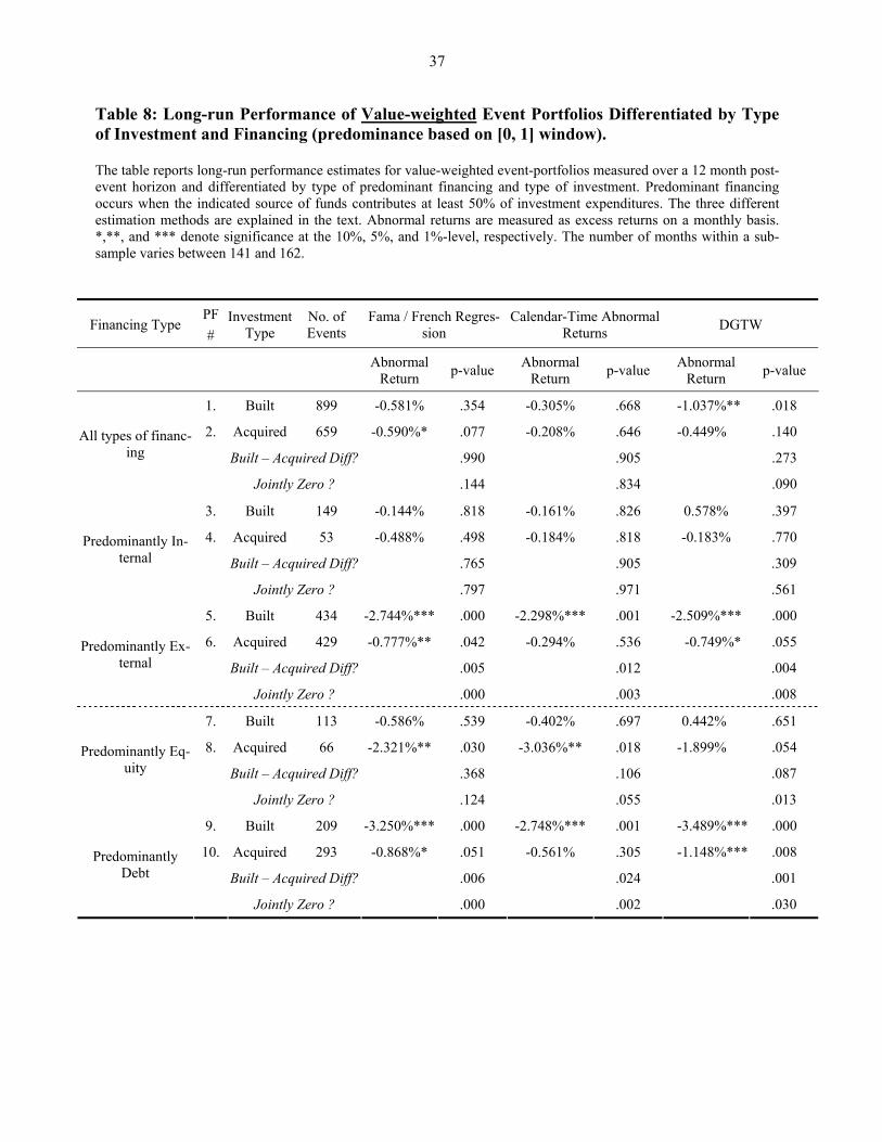
37

Table 8: Long-run Performance of Value-weighted Event Portfolios Differentiated by Type of Investment and Financing (predominance based on [0, 1] window). The table reports long-run performance estimates for value-weighted event-portfolios measured over a 12 month post-event horizon and differentiated by type of predominant financing and type of investment. Predominant financing occurs when the indicated source of funds contributes at least 50% of investment expenditures. The three different estimation methods are explained in the text. Abnormal returns are measured as excess returns on a monthly basis. *,**, and *** denote significance at the 10%, 5%, and 1%-level, respectively. The number of months within a sub-sample varies between 141 and 162.

Financing Type PF #

Investment Type

No. of Events

Fama / French Regres-sion

Calendar-Time Abnormal Returns DGTW

Abnormal Return p-value Abnormal

Return p-value Abnormal Return p-value

1. Built 899 -0.581% .354 -0.305% .668 -1.037%** .018

2. Acquired 659 -0.590%* .077 -0.208% .646 -0.449% .140

Built – Acquired Diff? .990 .905 .273 All types of financ-

ing

Jointly Zero ? .144 .834 .090

3. Built 149 -0.144% .818 -0.161% .826 0.578% .397

4. Acquired 53 -0.488% .498 -0.184% .818 -0.183% .770

Built – Acquired Diff? .765 .905 .309 Predominantly In-

ternal

Jointly Zero ? .797 .971 .561

5. Built 434 -2.744%*** .000 -2.298%*** .001 -2.509%*** .000

6. Acquired 429 -0.777%** .042 -0.294% .536 -0.749%* .055

Built – Acquired Diff? .005 .012 .004 Predominantly Ex-

ternal

Jointly Zero ? .000 .003 .008

7. Built 113 -0.586% .539 -0.402% .697 0.442% .651

8. Acquired 66 -2.321%** .030 -3.036%** .018 -1.899% .054

Built – Acquired Diff? .368 .106 .087 Predominantly Eq-

uity

Jointly Zero ? .124 .055 .013

9. Built 209 -3.250%*** .000 -2.748%*** .001 -3.489%*** .000

10. Acquired 293 -0.868%* .051 -0.561% .305 -1.148%*** .008

Built – Acquired Diff? .006 .024 .001 Predominantly

Debt

Jointly Zero ? .000 .002 .030

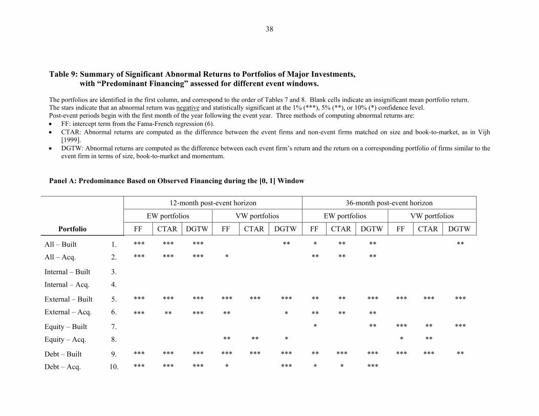
38

Table 9: Summary of Significant Abnormal Returns to Portfolios of Major Investments, with “Predominant Financing” assessed for different event windows. The portfolios are identified in the first column, and correspond to the order of Tables 7 and 8. Blank cells indicate an insignificant mean portfolio return. The stars indicate that an abnormal return was negative and statistically significant at the 1% (***), 5% (**), or 10% (*) confidence level. Post-event periods begin with the first month of the year following the event year. Three methods of computing abnormal returns are: • FF: intercept term from the Fama-French regression (6). • CTAR: Abnormal returns are computed as the difference between the event firms and non-event firms matched on size and book-to-market, as in Vijh

[1999]. • DGTW: Abnormal returns are computed as the difference between each event firm’s return and the return on a corresponding portfolio of firms similar to the

event firm in terms of size, book-to-market and momentum. Panel A: Predominance Based on Observed Financing during the [0, 1] Window

12-month post-event horizon 36-month post-event horizon

EW portfolios VW portfolios EW portfolios VW portfolios

Portfolio FF CTAR DGTW FF CTAR DGTW FF CTAR DGTW FF CTAR DGTW

All – Built 1. *** *** *** ** * ** ** **

All – Acq. 2. *** *** *** * ** ** **

Internal – Built 3.

Internal – Acq. 4.

External – Built 5. *** *** *** *** *** *** ** ** *** *** *** ***

External – Acq. 6. *** ** *** ** * ** ** **

Equity – Built 7. * ** *** ** ***

Equity – Acq. 8. ** ** * * **

Debt – Built 9. *** *** *** *** *** *** ** *** *** *** *** **

Debt – Acq. 10. *** *** *** * *** * * ***

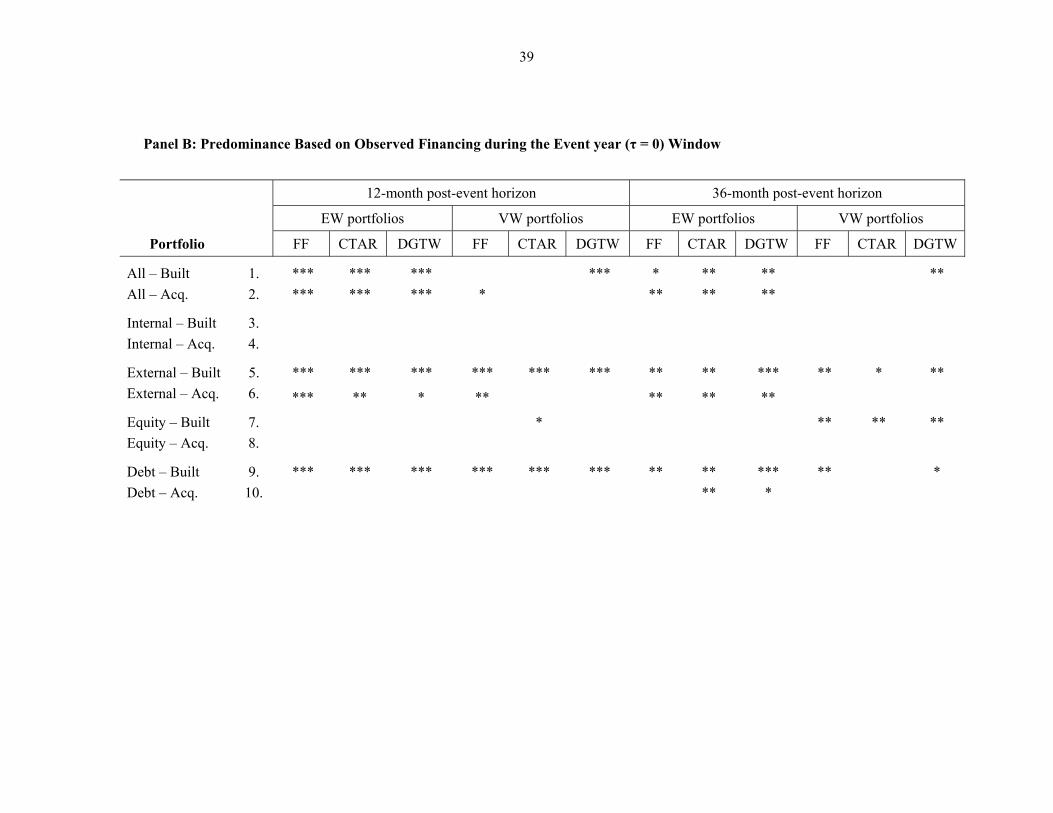
39

12-month post-event horizon 36-month post-event horizon

EW portfolios VW portfolios EW portfolios VW portfolios

Portfolio FF CTAR DGTW FF CTAR DGTW FF CTAR DGTW FF CTAR DGTW

All – Built 1. *** *** *** *** * ** ** ** All – Acq. 2. *** *** *** * ** ** **

Internal – Built 3. Internal – Acq. 4.

External – Built 5. *** *** *** *** *** *** ** ** *** ** * ** External – Acq. 6. *** ** * ** ** ** **

Equity – Built 7. * ** ** ** Equity – Acq. 8.

Debt – Built 9. *** *** *** *** *** *** ** ** *** ** * Debt – Acq. 10. ** *

Panel B: Predominance Based on Observed Financing during the Event year (τ = 0) Window

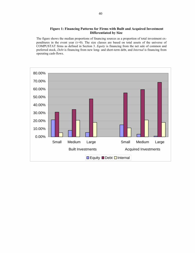
40

Figure 1: Financing Patterns for Firms with Built and Acquired Investment

Differentiated by Size The figure shows the median proportions of financing sources as a proportion of total investment ex-penditures in the event year (τ=0). The size classes are based on total assets of the universe of COMPUSTAT firms as defined in Section 3. Equity is financing from the net sale of common and preferred stock, Debt is financing from new long- and short-term debt, and Internal is financing from operating cash-flows.

0.00%

10.00%

20.00%

30.00%

40.00%

50.00%

60.00%

70.00%

80.00%

Small Medium Large Small Medium Large

Built Investments Acquired Investments

Equity Debt Internal

41

Appendix: Construction of Cash-Flow Financing Measures

The following table shows the exact definition of our financing measures. The scheme is based on Compustat’s “Statement of Cash Flows,” chapter 4 of the 2001 User’s Manual, pp. 15-16. Following Mayer and Sussman [2004], we assign zero values for missing data when a more aggregated item is present. For example, if there is a missing value for change in inventories (item 303), but the higher aggregate of operating activities – net cash flow (item 308) has a non-missing value, then we infer a zero value for change in inventories.

Sign Definition Compustat Data Item

Invest

+ Capital expenditures (“Built”) 128

+ Acquisitions (“Acquired”) 129

EQUITY

+ Sale of equity 108

- Purchase of equity 115

DEBT

+ Issuance of long-term debt 111

- Retirement of long-term debt 114

+ Change in current debt 301

INTERNAL CASH-FLOW (from operations)

+ After tax income before extraordinary items 123

+ Depreciation and amortization 125

- Cash dividends 127

OTHER

+ Sale of property, plant, equipment (book value) 107

+ Loss (gain) in sale of PPE and investments 213

42

+ Change in account payables and accrued liabilities 304

+ Change in accrued income taxes 305

+ Equity in net loss (earnings) 106

+ Extraordinary items 124

+ Other funds from operations 217

+ Exchange rate effect 314

+ Change in receivables 302

+ Deferred tax 126

+ Change in other assets and liabilities 307

+ Other financing 312

+ Other investment 310

- Increase in investment 113

+ Sale of investment 109

+ Increase in short-term investment 309

- Change in cash and equivalent 274

+ Change in inventory 303