Embed Size (px)
Citation preview
DEGREE PROJECT, IN RELIABILITY CENTRED ASSET MANAGEMENT FOR , SECOND LEVELELECTRICAL POWER SYSTEMS
STOCKHOLM, SWEDEN 2015
Maintenance Optimization Schedulingof Electric Power SystemsConsidering Renewable EnergySources
JIA YU
KTH ROYAL INSTITUTE OF TECHNOLOGY
SCHOOL OF ELECTRICAL ENGINEERING
Maintenance Optimization Scheduling of Electric Power Systems Considering
Renewable Energy Sources
Master Thesis Project Report
September 2015
Jia YU
Master of Electric Power Engineering Thesis 2015
KTH School of Electrical Engineering
Osquldas väg 10
SE-100 44 Stockholm

I
Master of Science Thesis MMK 2008:x {Track code} yyy
Maintenance Optimization Scheduling of Electric Power System Considering Renewable Energy Sources
Jia YU
Approved
2015-month-day
Examiner
Patrik Hilber
Supervisor
Ebrahim Shayesteh
Commissioner
{Name}
Contact person
{Name}
Abstract Maintenance is crucial in any industry to keep components in a reasonable functional condition, especially in electric power system, where maintenance is done so that the frequency and the duration of a fault can be shortened, thus increasing the availability of a certain component. And the reliability of the whole electric power system can also be improved. In the many deregulated electricity markets, reliability and economic driving forces are the two aspects that system operators mainly consider. It is expected for the system operator to provide consumers with the electricity of highest reliability and lowest cost. Therefore, in order to achieve this goal, providing the most economic maintenance schedule is vital in today’s power systems. One technique is Reliability Centred Maintenance (RCM), which is an effective method to maintain a certain level of reliability while carrying out maintenance schedules in an economic way. This thesis proposes an optimization problem for implementing the RCM method for a power system with renewable energy generators such as hydro power, wind power and solar panel generators. This aim is achieved through the following steps:
1- Literature review on power system reliability
2- Literature review on maintenance scheduling methods by focus on RCM method.
3- Compare the difference of conventional generators and renewable generators and model renewable generators in the power system.
4- Formulating the RCM method as an optimization problem.
5- The formulated model in 4 should be simulated for a test system using MATLAB.
6- The developed model in 5 is solved for different sets of available maintenance
II
strategies.
7- Summing all possible costs when different maintenance strategies are carried out and compare the costs. Choose the maintenance strategy with the lower cost to carry out the maintenance.

III
Acknowledge I would like express my greatest gratitude to my supervisor Ebrahim Shayesteh for his
continuous support and guidance throughout the execution of the whole master thesis
project. I would also like to give my thanks to Patrik Hilber for giving helpful
suggestions and guidance.
I would also like to thank Niklas Ekstedt, Per Westerlund from KTH and Leif Nilsson
from Ellevio for their valuable advices for my project and during my mid-presentation. I
would also like to thank my colleague Javi for his kind and patient explanation. And my
thanks also goes to Peter and Carin, for their generous help with the administrative
supportive work.
I would also like to thank my parents who have always given me supports in all aspects.
Finally, I would like to thank my friends who are always giving me strength when I meet
with difficulties in study and life.

IV
V
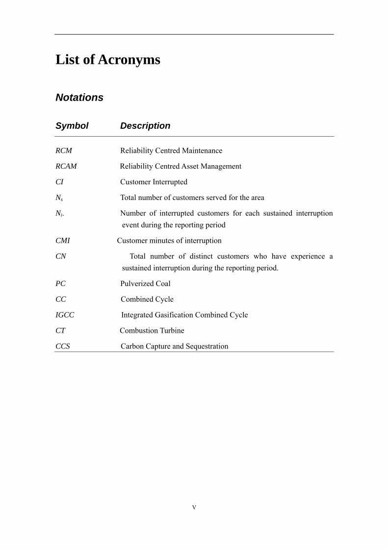
List of Acronyms
Notations
Symbol Description
RCM Reliability Centred Maintenance
RCAM Reliability Centred Asset Management
CI Customer Interrupted
Ns Total number of customers served for the area
Ni. Number of interrupted customers for each sustained interruption
event during the reporting period
CMI Customer minutes of interruption
CN Total number of distinct customers who have experience a
sustained interruption during the reporting period.
PC Pulverized Coal
CC Combined Cycle
IGCC Integrated Gasification Combined Cycle
CT Combustion Turbine
CCS Carbon Capture and Sequestration

VI
VII
Table of Content
Abstract .......................................................................................................................................... I
Acknowledge ............................................................................................................................... III
List of Acronyms .......................................................................................................................... V
Chapter 1 ....................................................................................................................................... 1
Introduction and Background ........................................................................................................ 1
1.1 Background and Motivation ................................................................................................ 1
1.2 Aim and Objectives ............................................................................................................. 2
1.3 Major Contributions ............................................................................................................ 2
1.4 Ethical aspects ..................................................................................................................... 3
1.5 Overview of the Report ....................................................................................................... 3
Chapter 2 ....................................................................................................................................... 5
Theory and Literature Review ....................................................................................................... 5
2.1 Understanding Power System Reliability............................................................................ 5
2.2 Capacity Outage Probability Table ..................................................................................... 7
2.3 Power Systems Reliability Evaluation Indices .................................................................... 8
2.3.1 Load Based Indices ...................................................................................................... 8
2.3.2 Customer Based Indices ............................................................................................... 9
2.4 Reliability Centred Maintenance (RCM) Brief ................................................................. 11
2.4.1 Definition and Brief background of RCM ................................................................. 11
2.4.2 Maintenance Alternatives in Past work of RCM ........................................................ 12
2.4.3 Types of Maintenance Strategies considered in RCM ............................................... 13
2.4.4 RCM logic .................................................................................................................. 15
2.5 Reliability Centred Asset Management (RCAM) Brief .................................................... 16
2.6 Severity Risk Index (SRI) from NERC ............................................................................. 18
2.7 Summary ........................................................................................................................... 21
Chapter 3 ..................................................................................................................................... 23
Methodology ............................................................................................................................... 23
3.1 Steps to be Carried Out ..................................................................................................... 23
VIII
3.2 RCM Simulation Logic and Contingency Description ..................................................... 25
3.3 Software MATPOWER ..................................................................................................... 27
3.4 IEEE 14-bus Test Network Description ............................................................................ 27
3.5 Improved IEEE 14-bus system with Distributed Generators ............................................ 29
3.5.1 Comparison Table of Conventional Generators and Renewable Generators ............. 29
3.5.2 Connecting voltage and capacity of distributed generators (solar, wind and hydro) . 31
3.5.3. IEEE Case 14-bus system with Distributed Generators ............................................ 33
3.6 Other Calculations ............................................................................................................. 35
3.6.1 EENS Calculating Model ........................................................................................... 35
3.6.2 SRI Calculation .......................................................................................................... 37
3.6.3 Operating and Interruption Cost ................................................................................. 40
3.6.4 Environmental Cost Calculation ................................................................................ 40
3.6.5 Maintenance Cost ....................................................................................................... 42
3.7 Summary ........................................................................................................................... 44
Chapter 4 ..................................................................................................................................... 45
Simulation Results and Discussion ............................................................................................. 45
4.1 Base Case ..................................................................................................................... 46
4.1.1 Without Renewable Generators.................................................................................. 46
4.1.2 With Renewable Generators ....................................................................................... 53
4.2 Sensitivity Simulation .................................................................................................. 59
4.2.1 Case 1: Increase Renewable Generator Capacity ....................................................... 59
4.2.2 Case 2: Increase Transmission Line Capacities ......................................................... 63
4.3 Summary ...................................................................................................................... 67
Chapter 5 ..................................................................................................................................... 68
Conclusions ................................................................................................................................. 68
Chapter 6 ..................................................................................................................................... 70
Recommendations and Future Work ........................................................................................... 70
References ................................................................................................................................... 72
Appendix ..................................................................................................................................... 76
Appendix I: MATPOWER Code for IEEE 14-bus system simulation ................................... 76
Appendix II: Input Data for Calculating SRI ........................................................................ 107
Appendix III: Simulation Results of Base Case .................................................................... 108

IX
Appendix IV: Simulation Results of Sensitivity Simulation Case 1 ..................................... 109
Appendix V: Simulation Results of Sensitivity Simulation Case 2 ...................................... 110

X
1
Chapter 1
Introduction and Background
1.1 Background and Motivation
Maintenance plays an important role in any field to maximize the lifecycle of a
component, but at the same time can cost a big fortune. Especially in today’s
deregulated electricity market, and system operators strive more to provide electricity
reliably and at the lowest cost the same time. However, it is a paradox sometimes that
more frequent maintenance does not necessarily help system operator to achieve goal
because of high cost of maintenance. And the cost of maintenance can not only be
assessed by its actual maintenance actions carried out, rather, the risk that taking a
component out for maintenance might bring to the system should also be considered
when assessing its maintenance cost [1]. A more efficient method to organize the
maintenance scheduling in an economic way while guarantying the power system
reliability is called for.
Reliability Centred Maintenance (RCM) was introduced in 1960’s and was later applied
to various fields. Some work have been done on RCM of electric power system, though
the more detailed approaches may differ, the basic logic of RCM is the same. In [2],
four cases from industry have been shown how the principle of RCM can be applied to
reach a balance between maintenance cost and reliability. A useful optimization method
in [3] for cost-efficient maintenance schedule for power distribution systems was
proposed. In [4], a developed computer program call RADPOW (Reliability Assessment
of Distributed Power Systems) was used for reliability evaluation and based on this, an
enhance RCM methodology was proposed. And in [5] a practical cost effective
methodology based on RCM was developed for an electric utility in Algeria.
RCM is designed to work together with traditional maintenance to guarantee the
reliability level, instead of replacing the traditional maintenance. Only Expected Energy
Not Supplied (EENS) or just the probability indices were considered when deciding
maintenance alternatives, but it is become more and more important to include other
factors, such as environmental and economic factors as well, even when deciding when
and how to carry out maintenance. Economic analysis including maintenance cost and
2
risk cost due to outages caused by maintenance, and interruption cost after maintenance,
should be considered in RCM analysis. [1]
1.2 Aim and Objectives
Aim:
The aim of this project is proposing an optimization problem for implementing RCM
for a power system with and without distributed generators. A set of maintenance
strategies for maintenance scheduling is defined, from which the best maintenance plan
considering both reliability and economic is selected. And the result of these two cases
with and without distributed generators are compared. Also study is done on two
sensitivity study cases where the capacity of the added renewable generators is
increased and the capacity of the transmission line is increased.
Objectives:
In order to achieve the aim above, the following objectives are completed:
1. Literature review on power system reliability are done.
2. Literature review on maintenance scheduling methods by focus on RCM method.
3. Compare the difference between conventional generators and renewable generators.
And model renewable generators in the power system.
4. Formulate the RCM method as an optimization problem.
5. The formulated model in 4 should be simulated for a test system using MATLAB.
6. The developed model in 5 is solved for different sets of available maintenance
strategies.
7. Summing all possible costs when different maintenance strategies are carried out
and compare the costs. Choose the maintenance strategy with the lower cost to carry
out the maintenance.
8. Repeat 4-7 for the power system with distributed generators included and choose the
best maintenance strategy for it.
1.3 Major Contributions
In this project, the basic RCM logic will be carried out with some other improvements
and enhancement. Following are the major contributions of this project:
1. When assessing the most critical component, Severity Risk Index (SRI) proposed by
North American Electric Reliability Corporation (NERC) was applied. SRI is used
because it focuses on the bulk power system (distribution and generation part in
power system), and it take into consideration of the impact on load loss, generation
3
loss, transmission line loss, and restoration speed, which is a comprehensive index
when evaluating the risk level of a component.
2. When selecting the best maintenance strategy, apart from comparing the
maintenance cost, the interruption cost, which reflect the risk of taking out a
component for maintenance are also considered. Furthermore, based on the ideology
that any development of human should not be at the cost of or at least should be at
the minimum cost of damaging the environment, environment cost is also included
in the total cost for comparing.
3. In today’s forming smart grid, distributed generators will play a more and more
important part. Including distributed generators into the power system for RCM
study gives us an idea of how distributed generators will affect the maintenance
strategy decision.
4. The simulation is done using MATPOWER, an embedded simulation package in
MATLAB for power flow and optimal power flow simulation. IEEE 14-bus system
obtained in MATPOWER is used for simulation.
1.4 Ethical aspects
The study of RCM will not only benefit system operators. With environmental cost
included in the total cost for each maintenance strategy, environmental impact are
considered. If a certain maintenance strategy results in, for example, a gas generator to
produce more electricity and therefore the emission of CO2 and other noxious gas, then
probably this maintenance strategy may not be the best choice. As the maintenance is
designed to be done based on reliability, the impact on consumers due to interruption is
reduced to the minimum level, thus human life and society will have the least loss. Also,
maintenance is done smarter, rather more frequently the better, labour and materials can
be saved and used more efficiently.
1.5 Overview of the Report
This report mainly focus on developing an optimization problem for RCM study on
power electricity system and it is divided into the following parts:
1. Introduction and Background: This part first introduces the nowadays situation of
electricity market and need for a smarter maintenance method. Aim and objectives
of this report is listed. Major contribution of this report is emphasised. Also the
ethical aspects of this report is state to reveal the importance of this study to human.
2. Theory and Literature Review: This part gives some basic theories of power system
4
reliability, and also the brief history and development of Reliability Centred
Maintenance (RCM). Further, some background information of Severity Risk Index
(SRI) proposed by North American Reliability Corporation (NERC) is provided.
3. Methodology: This part gives a detailed explanation of the methodology carried out
to achieve the aim and objectives of this project. The test network (IEEE 14-bus
system) with and without distributed generators are described. Also, the methods
used to calculate different types of cost, such as operation cost, interruption cost,
environmental cost and maintenance cost, are explained.
4. Simulation Results and Discussion: This part presents the simulation results of the
congested version of IEEE 14-bus system with and without renewable energy
generators (Base Case). Also two cases (Case 1, Case 2) for sensitivity study are
created and the corresponding results are shown here. Comparisons are made
between Case 1 and the Base case, and between Case 2 and the Base Case.
5. Conclusion: Conclusions are made based on the result obtained in chapter 4 and a
summary of all the results is presented.
6. Recommendations and Future Work: Some suggested future work is listed to make
this topic more comprehensive and closer to industry.
5
Chapter 2
Theory and Literature Review
This chapter gives theory and knowledge about power system reliability and the indices
such as load-based and customer-based indices for evaluating reliability of power
system is described. Also, brief review is done on Reliability Centred Maintenance and
Reliability Centred Asset Management. Lastly, Severity Risk Index proposed by North
American Electric Reliability Corporation’s (NERC) is introduced.
2.1 Understanding Power System Reliability
In today’s power system, it has been increasing vital to meet the demand of
customers, especially when the load is not fixed and may change in different
circumstances. Therefore the [6] function of power system, which is providing
electricity both reliably and economically is becoming more and more prominent.
To describe the reliability level of a bulk power system (mainly generation and
transmission parts), both deterministic and probabilistic methods are used in
complementary to each other and the ability of the system to satisfy the load
demand on a certain reliable level is assessed based on deterministic and
probabilistic indices [7].
One of the most commonly used deterministic method is the N-1 contingency
analysis, which means that the system will continue to operate without an
interruption of load supply when one element goes to outage [8]. Based on the past
performance of the elements in the bulk power system, and also weather conditions,
load diversity, generation dispatch, net scheduled interchange, the deterministic
assessment of the system is made [7]. However, in today’s deregulated electricity
market, where power demand and quality is variously changing, generation type is
diversified, rule & regulation can be changing [8], and deterministic method does
not take into account these uncertainties. This is where probabilistic methods come
into being, which can represent the random nature of power system.
The availability of a power system and the components that consist of the power
6
system can sometimes be affected by some random faults which is hard to predict
or controlled manually. And in order to quantize these kinds of affect, probabilistic
indices play an important role.
[6] To reasonably reflect the probabilistic and stochastic feature of power system,
the following aspects are considered:
Generating units can sometimes be outage and therefore, even if there are
plenty of reserve capacity installed, the possible risk level is not definitely
ensured lower.
The unavailability of transmission lines also has effect on the possibility of
supply interruption.
The constantly changing loading level, which is very likely different from the
load forecasted during planning period, has probabilistic impact on the
operation decisions.
In this project, the study of reliability degree is more focused on the bulk power
system, which is consisted mainly of generating units and transmission lines.
Therefore, the first two stochastic aspects are considered and their reliability and
economic impact on the IEEE case14 system are studied.
As pointed out in [6], the possibility of load shedding can be decreased by extra
consideration in respect of reliability during the planning period, operation period
or both. This project focus on looking for some smarter maintenance schedules or
maintenance schedule based on reliability, which can be counted as extra
consideration during operation period in order to decrease the probability and the
quantity of load shedding due to some random failures of components or part of the
system.
In order to keep a relatively reliable power system, certain parts of the system or
some components (generators and lines in this project) need to be maintained over a
period of time, and these maintenance actions will certainly generate a cost.
Meanwhile, if the components that have potential of going to outage is not
maintained in time, one or two components’ outage will likely to result in an
interruption of supply and the load shedding also generates an interruption cost. The
study on reliability can provide different average costs for reference to make better
operation decisions considering reliability and economy aspects. In this project,
smart maintenance schedule means maintenance decisions that keep a relatively
high reliability level of the power system at a lower or lowest cost.
7
2.2 Capacity Outage Probability Table
Capacity Outage Probability Table (COPT) [9] reflects the amount of electricity
that is not supplied in different states and the probability of each state. Since this
table has a lot to do with availability and unavailability, it is important to
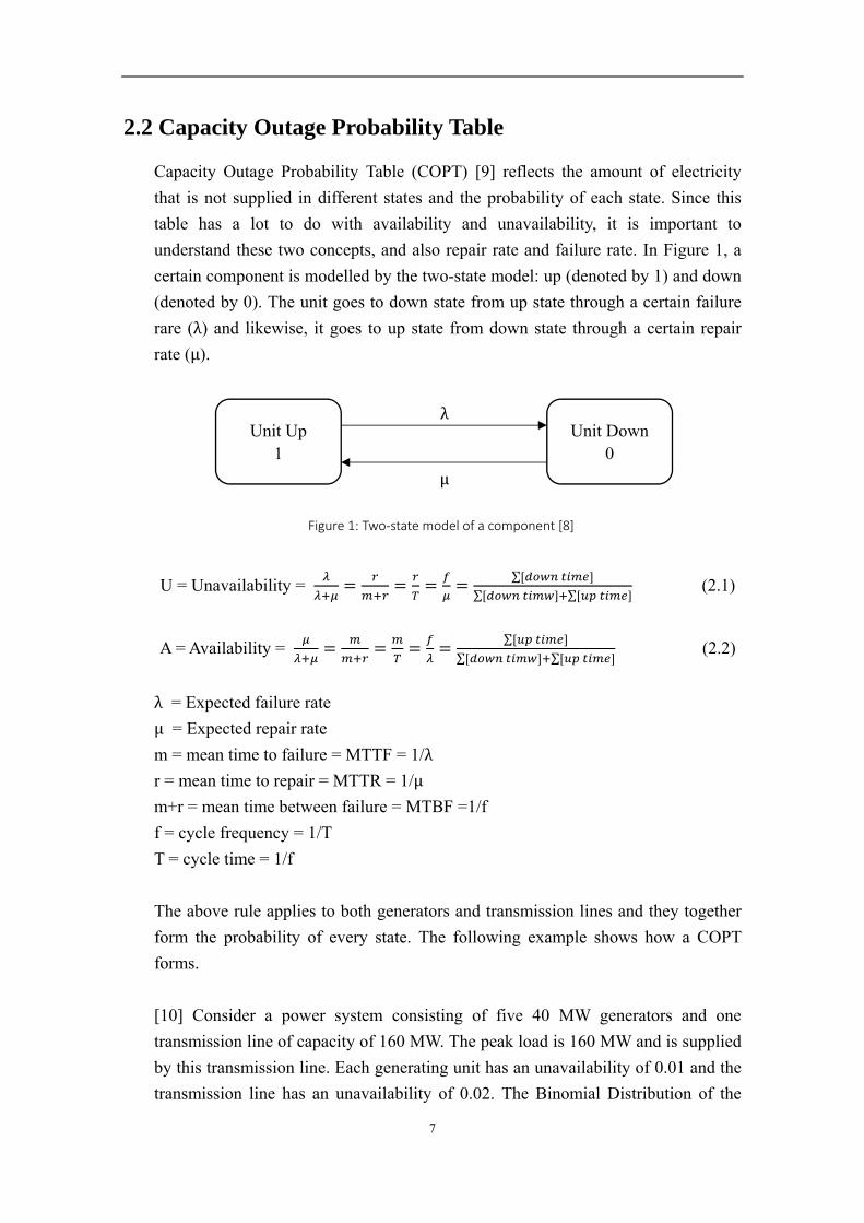
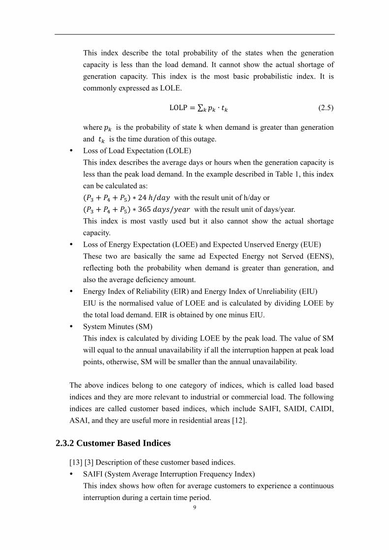
understand these two concepts, and also repair rate and failure rate. In Figure 1, a
certain component is modelled by the two-state model: up (denoted by 1) and down
(denoted by 0). The unit goes to down state from up state through a certain failure
rare (λ) and likewise, it goes to up state from down state through a certain repair
rate (μ).
U = Unavailability = ∑
∑ ∑ (2.1)
A = Availability = ∑
∑ ∑ (2.2)
λ = Expected failure rate
μ = Expected repair rate
m = mean time to failure = MTTF = 1/λ
r = mean time to repair = MTTR = 1/μ
m+r = mean time between failure = MTBF =1/f
f = cycle frequency = 1/T
T = cycle time = 1/f
The above rule applies to both generators and transmission lines and they together
form the probability of every state. The following example shows how a COPT
forms.
[10] Consider a power system consisting of five 40 MW generators and one
transmission line of capacity of 160 MW. The peak load is 160 MW and is supplied
by this transmission line. Each generating unit has an unavailability of 0.01 and the
transmission line has an unavailability of 0.02. The Binomial Distribution of the
Figure 1: Two‐state model of a component [8]
Unit Up 1
Unit Down 0
λ
μ
8
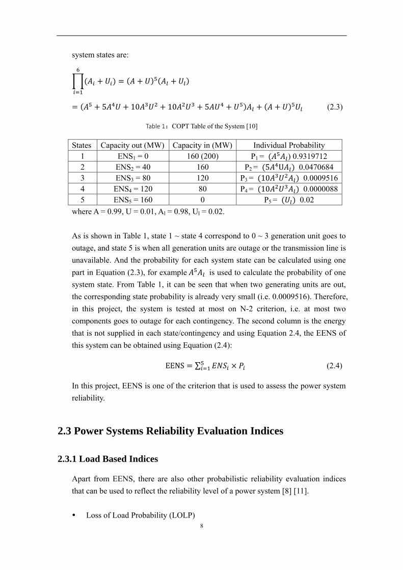
system states are:
5 10 10 5 (2.3)
Table 1:COPT Table of the System [10]
States Capacity out (MW) Capacity in (MW) Individual Probability 1 ENS1 = 0 160 (200) P1 = ) 0.9319712 2 ENS2 = 40 160 P2 = 5 U 0.0470684 3 ENS3 = 80 120 P3 = 10 0.0009516 4 ENS4 = 120 80 P4 = 10 0.0000088 5 ENS5 = 160 0 P5 = 0.02
where A = 0.99, U = 0.01, Al = 0.98, Ul = 0.02.
As is shown in Table 1, state 1 ~ state 4 correspond to 0 ~ 3 generation unit goes to
outage, and state 5 is when all generation units are outage or the transmission line is
unavailable. And the probability for each system state can be calculated using one
part in Equation (2.3), for example is used to calculate the probability of one
system state. From Table 1, it can be seen that when two generating units are out,
the corresponding state probability is already very small (i.e. 0.0009516). Therefore,
in this project, the system is tested at most on N-2 criterion, i.e. at most two
components goes to outage for each contingency. The second column is the energy
that is not supplied in each state/contingency and using Equation 2.4, the EENS of
this system can be obtained using Equation (2.4):
EENS ∑ (2.4)
In this project, EENS is one of the criterion that is used to assess the power system
reliability.
2.3 Power Systems Reliability Evaluation Indices
2.3.1 Load Based Indices
Apart from EENS, there are also other probabilistic reliability evaluation indices
that can be used to reflect the reliability level of a power system [8] [11].
Loss of Load Probability (LOLP)
9
This index describe the total probability of the states when the generation
capacity is less than the load demand. It cannot show the actual shortage of
generation capacity. This index is the most basic probabilistic index. It is
commonly expressed as LOLE.
LOLP ∑ ∙ (2.5)
where is the probability of state k when demand is greater than generation
and is the time duration of this outage.
Loss of Load Expectation (LOLE)
This index describes the average days or hours when the generation capacity is
less than the peak load demand. In the example described in Table 1, this index
can be calculated as:
∗ 24 / with the result unit of h/day or
∗ 365 / with the result unit of days/year.
This index is most vastly used but it also cannot show the actual shortage
capacity.
Loss of Energy Expectation (LOEE) and Expected Unserved Energy (EUE)
These two are basically the same ad Expected Energy not Served (EENS),
reflecting both the probability when demand is greater than generation, and
also the average deficiency amount.
Energy Index of Reliability (EIR) and Energy Index of Unreliability (EIU)
EIU is the normalised value of LOEE and is calculated by dividing LOEE by
the total load demand. EIR is obtained by one minus EIU.
System Minutes (SM)
This index is calculated by dividing LOEE by the peak load. The value of SM
will equal to the annual unavailability if all the interruption happen at peak load
points, otherwise, SM will be smaller than the annual unavailability.
The above indices belong to one category of indices, which is called load based
indices and they are more relevant to industrial or commercial load. The following
indices are called customer based indices, which include SAIFI, SAIDI, CAIDI,
ASAI, and they are useful more in residential areas [12].
2.3.2 Customer Based Indices
[13] [3] Description of these customer based indices.
SAIFI (System Average Interruption Frequency Index)
This index shows how often for average customers to experience a continuous
interruption during a certain time period.
10
SAIFI∑
∑ (2.6)
SAIDI (System Average Interruption Duration Index)
This index reflects the total length of time of the interruption of average
customer during a certain time period. This index is often measured in minutes
or hours.
SAIDI∑
∑ (2.7)
CAIDI (Customer Average Interruption Duration Index)
This index shows the average time period that is needed for the interruption to
be fixed and the service is restored.
CAIDI∑
∑ (2.8)
Or
CAIDI∑
∑ (2.9)
CAIFI (Customer Average Interruption Frequency Index)
This index shows the average frequency of continuous interruptions for the
customers that has the interruptions.
CAIFI∑
∑ (2.10)
ASAI (Average Service Availability Index)
This index shows an average time when customers get supplied during a
predefined time period.
ASAI∑
/ ∑
/ (2.11)
AENS (Average Energy Not Supplied)
AENS∑
(2.12)
11
2.4 Reliability Centred Maintenance (RCM) Brief
2.4.1 Definition and Brief background of RCM
RCM: A process used to determine what must be done to ensure that any physical
asset continues to do what its users want it to do in its present operating context –
From the book J.Moubray RCM [14]
Reliability Centred Maintenance was first mentioned and described in [15] by
F.Stanley Nowlan, Howard F.Heap. This maintenance process was first used in
aircraft industry in 1960’s when maintenance costs grew sharply as more and more
complicated equipment were put to practice to achieve different requirements [15].
What are the most important findings in [15] is that for many types of fault, for
example in aircraft industry, whether they happen or not has relatively little to do
with the level of maintenance that is done, and another valuable finding is that the
failure rates of some components do not necessarily increase the more they are used.
As a result of this, maintenance tasks based on the time might not have the most
effective impact on guaranteeing components’ availability.
Since its appearance, RCM has been applied in different industries, like aircraft and
aerospace industry, nuclear industry, shipping, chemical industries, process/oil &
gas, small and medium companies, hospital and water distribution companies [16].
Later, RCM was also applied in electrical engineering systems. Some studies of
RCM application has been done for components level [17] [18] and also
distribution system level [19].
Like in the aircraft industry, where components or systems of great importance
often have redundancy in case of a fault and these crucial functions will still be
available [15], there is also redundancy of electricity generation in today’s more
and more reliable power systems. In some of the advanced power systems, like in
Singapore, the total capacity is about more than 30% higher than the maximum
demand. In these types of power systems, it seems that whether carrying out
Reliability Centred Maintenance or not does not affect the reliability and economic
benefit of this power system from the whole society’s view. But in more congested
power systems, when and how to carry out the maintenance tasks will have impact
on the system reliability and the related expenses.
Therefore, in some of the congested power systems, it has become crucial to
schedule maintenance plans so that the reliability of the system is maintained at an
12
acceptable level while keeping the related costs minimum. Also, deregulation in
today’s power system market has urged system operators to provide customers with
the most economic maintenance schedule which has the least impact on the
reliability of power delivery.
All these driving factors in today’s deregulated power system market had called for
[20] an efficient method to schedule a maintenance plan in an economic way while
maintaining a certain level of reliability. In this report, Reliability Centred
Maintenance (RCM) is used achieve this goal.
2.4.2 Maintenance Alternatives in Past work of RCM
RCM can cover various areas and the specific techniques and evaluation methods may
vary between different application areas. In RCM, instead of deciding carrying out
maintenance or not based on the components’ capital cost, it focuses more on the
damage that may be brought to the whole power system when taking out this
components for maintenance [1].
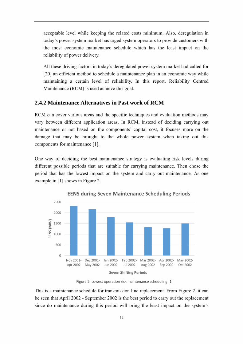
One way of deciding the best maintenance strategy is evaluating risk levels during
different possible periods that are suitable for carrying maintenance. Then chose the
period that has the lowest impact on the system and carry out maintenance. As one
example in [1] shows in Figure 2.
This is a maintenance schedule for transmission line replacement. From Figure 2, it can
be seen that April 2002 - September 2002 is the best period to carry out the replacement
since do maintenance during this period will bring the least impact on the system’s
Figure 2: Lowest operation risk maintenance scheduling [1]
0
500
1000
1500
2000
2500
Nov 2001‐Apr 2002
Dec 2001‐May 2002
Jan 2002‐Jun 2002
Feb 2002‐Jul 2002
Mar 2002‐Aug 2002
Apr 2002‐Sep 2002
May 2002‐Oct 2002
EENS (M
W)
Seven Shifting Periods
EENS during Seven Maintenance Scheduling Periods
13
reliability level. Deciding when to carry out maintenance is only a part of RCM scheme.
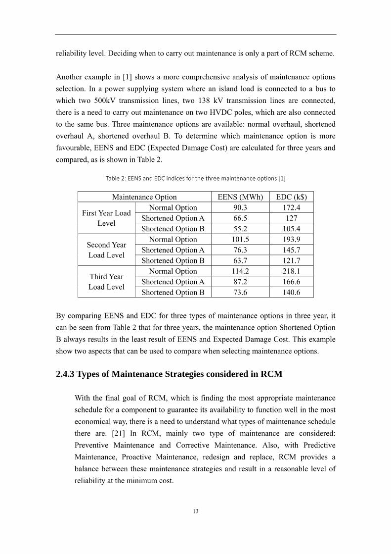
Another example in [1] shows a more comprehensive analysis of maintenance options
selection. In a power supplying system where an island load is connected to a bus to
which two 500kV transmission lines, two 138 kV transmission lines are connected,
there is a need to carry out maintenance on two HVDC poles, which are also connected
to the same bus. Three maintenance options are available: normal overhaul, shortened
overhaul A, shortened overhaul B. To determine which maintenance option is more
favourable, EENS and EDC (Expected Damage Cost) are calculated for three years and
compared, as is shown in Table 2.
Table 2: EENS and EDC indices for the three maintenance options [1]
Maintenance Option EENS (MWh) EDC (k$)
First Year Load Level
Normal Option 90.3 172.4 Shortened Option A 66.5 127 Shortened Option B 55.2 105.4
Second Year Load Level
Normal Option 101.5 193.9 Shortened Option A 76.3 145.7 Shortened Option B 63.7 121.7
Third Year Load Level
Normal Option 114.2 218.1 Shortened Option A 87.2 166.6 Shortened Option B 73.6 140.6
By comparing EENS and EDC for three types of maintenance options in three year, it
can be seen from Table 2 that for three years, the maintenance option Shortened Option
B always results in the least result of EENS and Expected Damage Cost. This example
show two aspects that can be used to compare when selecting maintenance options.
2.4.3 Types of Maintenance Strategies considered in RCM
With the final goal of RCM, which is finding the most appropriate maintenance
schedule for a component to guarantee its availability to function well in the most
economical way, there is a need to understand what types of maintenance schedule
there are. [21] In RCM, mainly two type of maintenance are considered:
Preventive Maintenance and Corrective Maintenance. Also, with Predictive
Maintenance, Proactive Maintenance, redesign and replace, RCM provides a
balance between these maintenance strategies and result in a reasonable level of
reliability at the minimum cost.
14
1). Preventive Maintenance (PM)
[22] This type of maintenance is carried out on a predetermined time interval
(clock time, cycles, calendar days, seasons of the year or prior to some events)
without considering the actual condition of the component. Certain maintenance
tasks such as, checking, cleaning, lubrication, tighten, test and replacement a
component can be carried out in PM before a failure actually happens and the
failure rate of the components is reduced in this way. More often, preventive
maintenance is done for the components of higher importance in power system
[15]. Time-directed maintenance is one type of Preventive Maintenance.
2). Corrective Maintenance (CM)
[23] This type of maintenance is done to a failed equipment, machine, or system
to restore them to the operating condition that satisfies the tolerances or limits.
This type of maintenance is more effective when the cost of PM maintenance is
greater than the cumulative cost of a certain fault or when no appropriate PM
actions exist [24]. This type of maintenance is mainly applied to less important
components in power system [15]. Failure Finding (FF) is one of this type of
maintenance and it is to inspect the equipment on a schedule basis, and when
hidden failure is found, corrective maintenance is initiated. Run-to-failure
Maintenance (RTF) is to fix the equipment when it fails without any scheduled
maintenance.
Both FF and RTF equal to perform no maintenance before a failure happens
because no possible PM maintenance actions can be found or because of the
economical factor.
3). Predictive Maintenance and Real-Time Monitoring
[22] In Predictive Maintenance, equipment is inspected on schedule or ongoing
basis to find any potential failure, indicated by measured condition data, is to
happen in the future. If the equipment is found to be about to fail, preventive
maintenance is initiated. Real-time Monitoring, as its name reveals, utilises
real-time performance data to evaluate the condition of a component or machine.
Condition-based maintenance (CBM) is one type of Preventive Maintenance.
Since in [15], it is pointed out that Preventive Maintenance will not necessarily
make a significant increase in reliability and often with a high inspection and
maintenance cost, CBM is gradually becoming more attractive than Preventive
Maintenance.
15
2.4.4 RCM logic
In [15], the key process of carrying out RCM is described in the following steps:
1). Classify components into different groups and identify those that need more
complex study on its maintenance schedule (components like fuse does not need
very complicated maintenance as they normally run-to-failure and then gets
replaced).
2). Further identify critical components that have potential function failure that
will cause safety or economic losses, so that they need maintenance schedule
beforehand.
3). Based on the potential failure consequences of the components identified in
step 2), evaluate different maintenance actions and requirements (reliability or
economical requirements). And select the tasks that fulfil the requirements.
4). For the items that no appropriate maintenance actions can be found, suggestion
such as no maintenance for the time being and design changing (if no
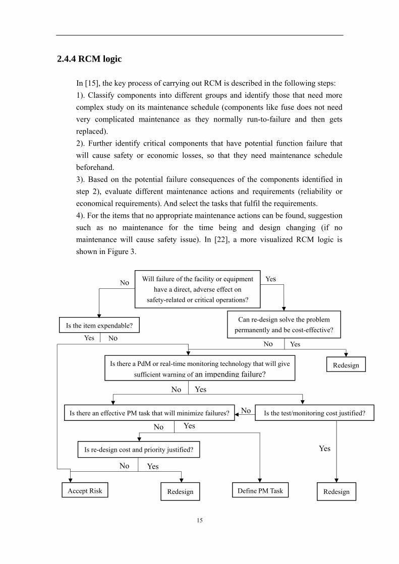
maintenance will cause safety issue). In [22], a more visualized RCM logic is
shown in Figure 3.
Redesign
Can re-design solve the problem
permanently and be cost-effective?
No Yes
No Yes
No
Yes
Yes No
Yes No
No Yes
No Will failure of the facility or equipment
have a direct, adverse effect on
safety-related or critical operations?
Is the item expendable?
Is there a PdM or real-time monitoring technology that will give
sufficient warning of an impending failure?
Is there an effective PM task that will minimize failures? Is the test/monitoring cost justified?
Is re-design cost and priority justified?
Accept Risk Redesign Define PM Task Redesign
Yes
16
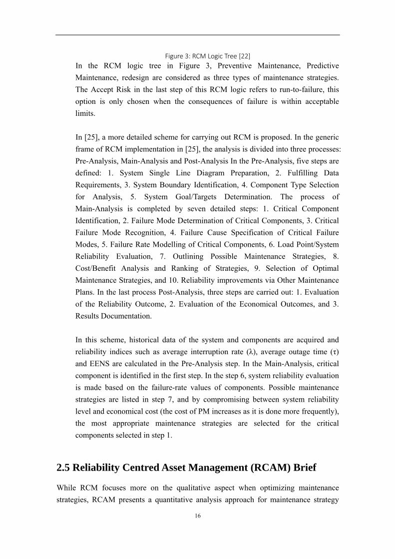
In the RCM logic tree in Figure 3, Preventive Maintenance, Predictive
Maintenance, redesign are considered as three types of maintenance strategies.
The Accept Risk in the last step of this RCM logic refers to run-to-failure, this
option is only chosen when the consequences of failure is within acceptable
limits.
In [25], a more detailed scheme for carrying out RCM is proposed. In the generic
frame of RCM implementation in [25], the analysis is divided into three processes:
Pre-Analysis, Main-Analysis and Post-Analysis In the Pre-Analysis, five steps are
defined: 1. System Single Line Diagram Preparation, 2. Fulfilling Data
Requirements, 3. System Boundary Identification, 4. Component Type Selection
for Analysis, 5. System Goal/Targets Determination. The process of
Main-Analysis is completed by seven detailed steps: 1. Critical Component
Identification, 2. Failure Mode Determination of Critical Components, 3. Critical
Failure Mode Recognition, 4. Failure Cause Specification of Critical Failure
Modes, 5. Failure Rate Modelling of Critical Components, 6. Load Point/System
Reliability Evaluation, 7. Outlining Possible Maintenance Strategies, 8.
Cost/Benefit Analysis and Ranking of Strategies, 9. Selection of Optimal
Maintenance Strategies, and 10. Reliability improvements via Other Maintenance
Plans. In the last process Post-Analysis, three steps are carried out: 1. Evaluation
of the Reliability Outcome, 2. Evaluation of the Economical Outcomes, and 3.
Results Documentation.
In this scheme, historical data of the system and components are acquired and
reliability indices such as average interruption rate (λ), average outage time (τ)
and EENS are calculated in the Pre-Analysis step. In the Main-Analysis, critical
component is identified in the first step. In the step 6, system reliability evaluation
is made based on the failure-rate values of components. Possible maintenance
strategies are listed in step 7, and by compromising between system reliability
level and economical cost (the cost of PM increases as it is done more frequently),
the most appropriate maintenance strategies are selected for the critical
components selected in step 1.
2.5 Reliability Centred Asset Management (RCAM) Brief
While RCM focuses more on the qualitative aspect when optimizing maintenance
strategies, RCAM presents a quantitative analysis approach for maintenance strategy
Figure 3: RCM Logic Tree [22]
17
optimization [44]. RCAM consists two parts: RCM and Quantitative Maintenance
Optimization (QMO). QMO takes into consideration of the total cost and possible
benefit brought by a certain maintenance, such that the right decisions of which type of
maintenance to be carried out at the lowest cost can be made [45]. RCAM combines
both the quantitative analysis of RCM and the qualitative analysis of QMO, thus
ensuring the most appropriate maintenance is done on the required component in the
most cost effectively way considering the system reliability [44]. The concept of RCAM
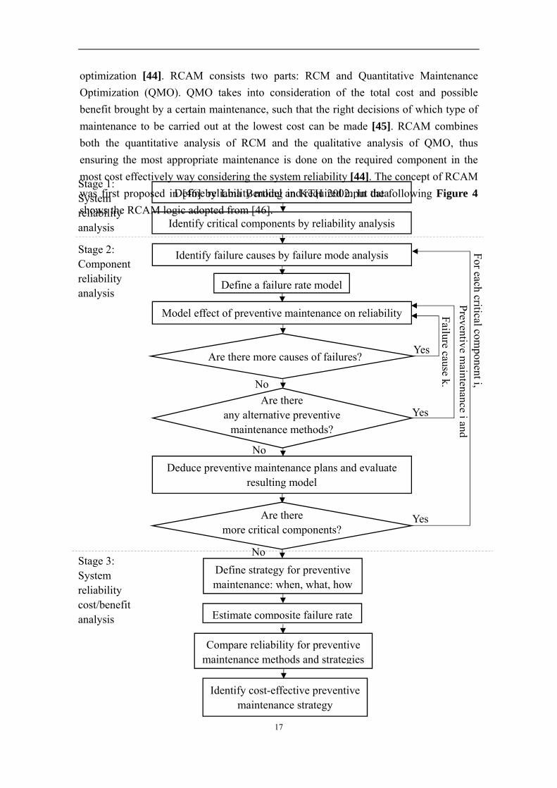
was first proposed in [46] by Lina Bertling in KTH 2002. In the following Figure 4
shows the RCAM logic adopted from [46].
Stage 1: System reliability analysis
Stage 2: Component reliability analysis
Deduce preventive maintenance plans and evaluate resulting model
Are there
more critical components?
Define strategy for preventive maintenance: when, what, how
Estimate composite failure rate
Compare reliability for preventive maintenance methods and strategies
Identify cost-effective preventive maintenance strategy
Define reliability model and required input data
Identify critical components by reliability analysis
Identify failure causes by failure mode analysis
Define a failure rate model
Model effect of preventive maintenance on reliability
Are there more causes of failures?
Are there any alternative preventive
maintenance methods?
Yes
Yes
Preventive
maintenance
jand
Failure
causek.
For each critical com
ponent i,
Yes
No
No
No
Stage 3: System reliability cost/benefit analysis
18
In the Stage 1, the reliability of the studied system is analysed base on the input data
including testing network data, customer data, and components historical reliability data.
Also the most critical component is identified in Stage 1. In Stage 2, each critical
component is studied more in details based on their historical input data. Also study is
done for the impact of different types of preventive maintenance of components’ failure.
In the last stage, the results of maintenance for components are compared in a system
level from the aspects of cost and reliability.
2.6 Severity Risk Index (SRI) from NERC
There have been some researches on the indices that can reflect the severity level in
a system or of a component. In this project, the Severity Risk Index proposed by
North American Electric Reliability Corporation’s (NERC) Operating Committee
(OC) and Planning Committee (PC) in 2010 [26], is used to assess the importance
level of different components and the most critical one is selected based on the
ranking list of the SRI of each components. This is a very important step in the
whole logic of RCM of this project as the maintenance schedule carried out later is
based on the decision in this step.
There have been two versions of SRI defined by NERC. The first one, as will be
called SRIOLD1 from now on, integrates the impact of different events from
transmission level, generation level and also load level. By assigning different
weighting values from industrial experience, the value of this risk index can be
calculated with transmission loss, generation loss and load shedding all blended in,
resulting in a single value [27]. SRIOLD1 was fist defined as the following [28]:
SRI ∗ ∗ ∗ ∗ ∗ (2.13)
Where
SRI = severity risk index for specific event,
= weighting of load loss,
= normalized MW of Load Loss in percent,
= weighting of transmission line lost,
= normalized number of transmission lines lost in percent,
= weighting of generators lost,
= normalized number of generators lost in percent,
Figure 4: Reliability Centered Asset Management (RCAM) Logic [46]
19
= weighting of duration of event,
= normalized duration of the event in percent,
= weighting of equipment damage,
= normalized number of equipment damaged in percent.
[28] Reliability Metrics Working Group (RMWG) later decided that transmission,
generation and load losses are more important, and at the same time the duration of
load loss should also somehow incorporated in this Severity Risk Index. Below
shows the refined version of SRIOLD2.
SRI ∗ ∗ ∗ ∗ (2.14)
SRI = severity risk index for specific event (span a day),
= 60%,
= normalized MW of Load Loss in percent,
= 30%,
= normalized number of transmission lines lost in percent,
= 10%,
= normalized number of generators lost in percent,
RPL = load Restoration Promptness Level:
RPL = 1/3, if restoration < 4 hours,
RPL = 2/3, if 4 <= restoration < 12 hours,
RPL = 3/3, if restoration >= 12 hours
In this refined version of SRIOLD2, according to industrial experience, different
weighting are set for load loss, transmission loss and generation loss. And
interruption duration is included in SRI using RPL depending on different
restoration hour.
In this project SRIbps, which is a further refinement of SRI, is used to assess the risk
severity level of an event and its impact on the system reliability. Regarding the
load loss part in SRIOLD2, whether the load loss is a result a fault at transmission
level or generation level, or an outage in the distribution level causes the load loss
is not taken into consideration. SRIbps gives better evaluation of the risk severity
level of events that cause load shedding due to an interruption of supply in
transmission or generation level, instead of fault in the distribution facilities [26].
The subscript bps stands for Bulk Power System, which is a interconnect power
system that consists of transmission and generation facilities, and does not include
facilities used for distribution purpose [29].
20
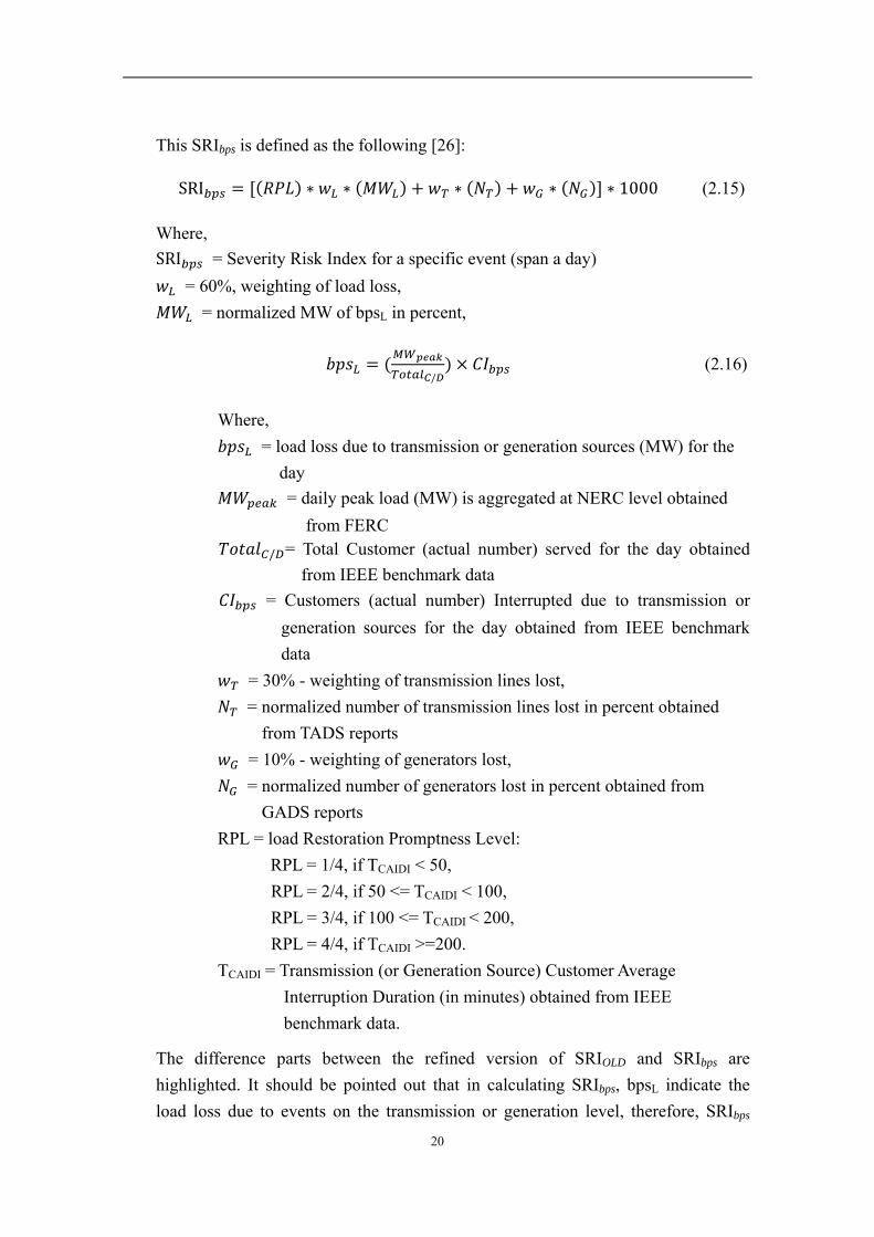
This SRIbps is defined as the following [26]:
SRI ∗ ∗ ∗ ∗ ∗ 1000 (2.15)
Where,
SRI = Severity Risk Index for a specific event (span a day)
= 60%, weighting of load loss,
= normalized MW of bpsL in percent,
/
(2.16)
Where,
= load loss due to transmission or generation sources (MW) for the
day
= daily peak load (MW) is aggregated at NERC level obtained
from FERC
/ = Total Customer (actual number) served for the day obtained
from IEEE benchmark data
= Customers (actual number) Interrupted due to transmission or
generation sources for the day obtained from IEEE benchmark
data
= 30% - weighting of transmission lines lost,
= normalized number of transmission lines lost in percent obtained
from TADS reports
= 10% - weighting of generators lost,
= normalized number of generators lost in percent obtained from
GADS reports
RPL = load Restoration Promptness Level:
RPL = 1/4, if TCAIDI < 50,
RPL = 2/4, if 50 <= TCAIDI < 100,
RPL = 3/4, if 100 <= TCAIDI < 200,
RPL = 4/4, if TCAIDI >=200.
TCAIDI = Transmission (or Generation Source) Customer Average
Interruption Duration (in minutes) obtained from IEEE
benchmark data.
The difference parts between the refined version of SRIOLD and SRIbps are
highlighted. It should be pointed out that in calculating SRIbps, bpsL indicate the
load loss due to events on the transmission or generation level, therefore, SRIbps
21
differentiate impact of transmission or generation (bulk power system) related
events from that resulting from both bulk power system and distribution system.
Since in this project, transmission line and generation losses are mainly considered,
SRIbps is more suitable to assess the severity risk level of each event, or more
specifically, of each component.
2.7 Summary
In Chapter 2, knowledge and importance of power system reliability was given first
and the way of calculating EENS was explained. Further, load-based and
customer-based reliability indices were given as ways to evaluate reliability of
power system. Then, the history and types of maintenance strategies of Reliability
Centred Maintenance (RCM) was elaborated. Also, some examples of RCM logic
were given for better understanding of the core of this project. Description of
Reliability Centred Asset Management (RCAM) and its relation with RCM were
introduced. At last, the development and calculation of Severity Risk Index, which
is used in this project for assessing the severity of each component/event, was
introduced as the last part of this chapter.

22
23
Chapter 3
Methodology
This chapter first presents a list of descriptions for all the tasks that are needed to fulfil
the overall aim, which is proposing an optimization problem for maintenance strategy
selection for a power system with and without including renewable energy generators
by using RCM method. Then the simulation logic for carrying out all the tasks and
contingencies that are considered in the logic are described. The testing system IEEE
14-bus system with and without renewable generator added are described. Finally,
calculation of SRI value of all the components, operation & interruption cost during and
after maintenance, environmental cost during and after maintenance, and maintenance
cost for both generators and transmission lines.
3.1 Steps to be Carried Out
In order to achieve the overall aim of proposing an optimization problem for
maintenance scheduling of an electric power system, with renewable energy generators
integrated, by implementing RCM method, the following steps have been carried out.
(a) In order to integrate distributed generators into the existing power system, some
comparisons between conventional generators and renewable generators are made to
differentiate their differences.
(b) Based on the differences found in the (a), some of the differences that matter more
in the study of RCM are selected and renewable energy generators are modelled and
then added to IEEE 14-bus system.
(c) To have a more suitable power system for RCM study, both the original IEEE
14-bus power system and the one that has renewable generators integrated are made
more congested by increasing load amount and decrease generation capacity
reasonably.
(d) RCM is first studied on the power system without renewable energy generator.
Using Severity Risk Index proposed by NERC to assess the risk level of each
24
component (generators or transmission lines) and select the one with the highest SRI
value. In this project, generators and transmission lines are studied separately for
RCM. Therefore, one generator and one transmission line, both have highest SRI
value among all generators or all transmission lines, are selected.
(e) Calculate the average operation & interruption cost, environmental cost,
maintenance cost during the maintenance done on the generator and line selected in
(d) under different contingencies. In this project, three levels (100%, 50%, and 0%)
of maintenance have been considered and they are differentiated by the spanning
period of time.
(f) Calculate the average operation & interruption cost and environmental cost after
different levels of maintenance done on generator and line under different
contingencies. The total spanning period of time is selected as one year, therefore
the period after maintenance is one year minus the maintenance period in (e).
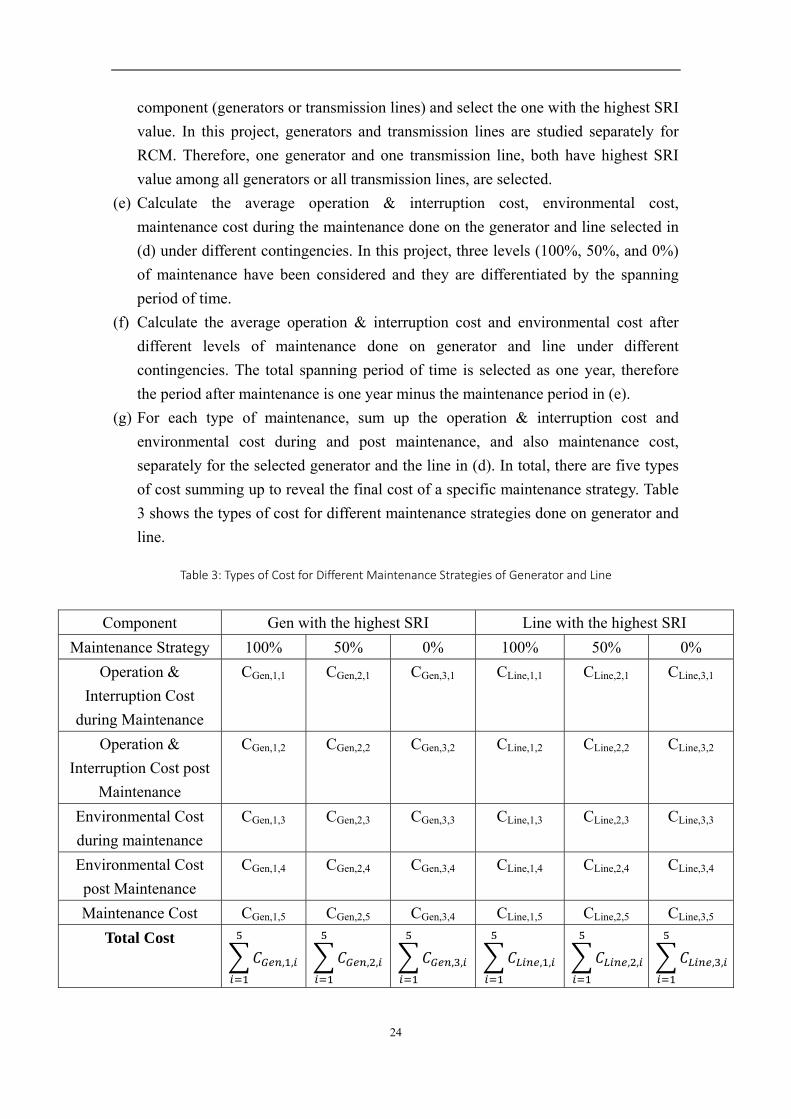
(g) For each type of maintenance, sum up the operation & interruption cost and
environmental cost during and post maintenance, and also maintenance cost,
separately for the selected generator and the line in (d). In total, there are five types
of cost summing up to reveal the final cost of a specific maintenance strategy. Table
3 shows the types of cost for different maintenance strategies done on generator and
line.
Table 3: Types of Cost for Different Maintenance Strategies of Generator and Line
Component Gen with the highest SRI Line with the highest SRI
Maintenance Strategy 100% 50% 0% 100% 50% 0%
Operation &
Interruption Cost
during Maintenance
CGen,1,1 CGen,2,1 CGen,3,1 CLine,1,1 CLine,2,1 CLine,3,1
Operation &
Interruption Cost post
Maintenance
CGen,1,2 CGen,2,2 CGen,3,2 CLine,1,2 CLine,2,2 CLine,3,2
Environmental Cost
during maintenance
CGen,1,3 CGen,2,3 CGen,3,3 CLine,1,3 CLine,2,3 CLine,3,3
Environmental Cost
post Maintenance
CGen,1,4 CGen,2,4 CGen,3,4 CLine,1,4 CLine,2,4 CLine,3,4
Maintenance Cost CGen,1,5 CGen,2,5 CGen,3,4 CLine,1,5 CLine,2,5 CLine,3,5
Total Cost
, , , , , , , , , , , ,
25
(h) By ranking the total cost of different maintenance strategies, select the one with the
lowest cost and carry out the corresponding maintenance for the generator or
transmission line.
(i) Repeat steps (d) – (h) for the IEEE 14-bus system (congested version) with
distributed generators integrated.
(j) A cost result table similar to Table 3 is obtained and the best maintenance strategy
with the minimum total cost for generator or line in the power system with
distributed generator integrated can be selected.
(k) Compare the results obtained in (h) and (j) to see what kind of difference will be
brought about to the maintenance strategies before and after including distributed
generators. And also compare other results like EENS, average loading of generators
or transmission lines, voltage level on each bus.
(l) For sensitivity study, a case (Case 1) is created with a larger renewable energy
generation capacity and other input data unchanged. Repeat steps (d) – (h) for Case
1 with renewable generators. Compare the results obtained with that obtained in (h)
for the congested version of IEEE 14-bus system with renewable generators.
(m) In Sensitivity study, another case (Case 2) is created with higher transmission line
capacity and other input data unchanged. Repeat steps (d) – (h) for Case 1 with and
without renewable generators. Compare the results obtained for Case 2 with the
corresponding results obtained for the Base Case.
3.2 RCM Simulation Logic and Contingency Description
Figure 5 shows the flow chart of simulation logic in MATPOWER. As can be seen in
Figure 5, two main part of simulation have been done, one for the maintenance period
and the other for the after maintenance period. In this project, the total study period is
one year. Depending on the different maintenance levels, 100% maintenance
corresponds to four weeks’ time period, 50% maintenance corresponds to two weeks’
time, and 0% maintenance equals to zero week.
For contingencies during maintenance, at most two components go to outage are
considered. More specifically, when maintenance is done on the generator with the
highest SRI (Gen), the first contingency considered is none of the component is
unavailable. Then, the Gen is set to be outage, the rest components (generators apart
from the Gen and all the transmission lines) are set to be outage one by one and one at a
time, resulting in 1+(number of generators-1)+(number of lines) contingencies. While
when maintenance is done on the line with the highest SRI (Line), the first contingency
is still none of the components is unavailable. Then, the Line is set to be outage, the rest
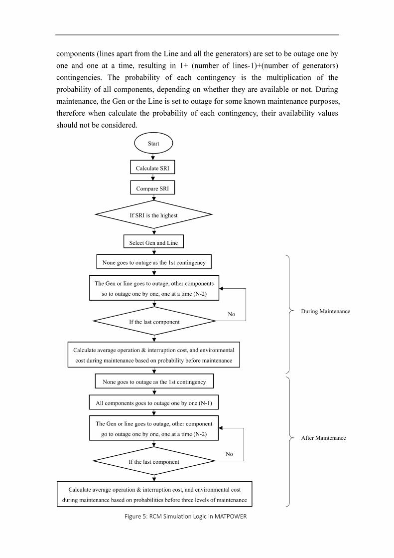
26
components (lines apart from the Line and all the generators) are set to be outage one by
one and one at a time, resulting in 1+ (number of lines-1)+(number of generators)
contingencies. The probability of each contingency is the multiplication of the
probability of all components, depending on whether they are available or not. During
maintenance, the Gen or the Line is set to outage for some known maintenance purposes,
therefore when calculate the probability of each contingency, their availability values
should not be considered.
After Maintenance
During Maintenance
If the last component
Calculate average operation & interruption cost, and environmental cost
during maintenance based on probabilities before three levels of maintenance
The Gen or line goes to outage, other components
so to outage one by one, one at a time (N-2)
Calculate average operation & interruption cost, and environmental
cost during maintenance based on probability before maintenance
If the last component
None goes to outage as the 1st contingency
All components goes to outage one by one (N-1)
The Gen or line goes to outage, other component
go to outage one by one, one at a time (N-2)
Start
Calculate SRI
If SRI is the highest
Select Gen and Line
Compare SRI
None goes to outage as the 1st contingency
No
No
Figure 5: RCM Simulation Logic in MATPOWER
27
Likewise, for contingencies after maintenance is done on generator or line, in order to
consider as many contingencies with relatively high probability as possible, there are in
total 2*(number of generators + number of lines) contingencies. Taking the Gen for
which maintenance is done as an example, the first contingency is none of the
components go to outage. Then all components including all the transmission lines and
generators go to outage one by one and one at a time. After this, the Gen is set to outage,
then the rest of the components go to outage one by one and one at a time. Unlike the
probability during maintenance, when calculating probability of each contingency post
maintenance, the availability values of the Gen and the Line are considered. The similar
simulation logic is set for the Line. For more details, please refer to the MATPOWER
code in Appendix I. The probability of each components is assumed to be improved as
the level of maintenance increases. Therefore, the same contingency will have different
probabilities in different maintenance degrees.
3.3 Software MATPOWER
In this project MATPOWER is used. MATPOWER is a package of Matlab for solving
power flow (pf) and optimal power flow (opf) problems [30]. Optimal power flow is
used in this project since guarantee reliability level at the minimum cost the one of the
important incentive or RCM. MATPOWER is used in this project because it is easier to
carry out opf for different contingencies in a loop and all the results can be obtained
through one programme by calling other embedded functions. But also due to this, when
opf of a contingency does not converge, it is more difficult to check what goes wrong
and correct it, which can be one limit of this project. Throughout the whole project, it is
found that MATPOWER 5.0v does not work so well with all the contingencies
considered in this project. Therefore, MATPWOER 3.2v is used instead, although the
speed is a little slower than 5.0v. In this project, every contingency converges and
solutions of opf have been found all contingencies.
3.4 IEEE 14-bus Test Network Description
In this project, IEEE 14-bus power system retrieved from MATPOWER is used for
RCM study. As discussed in 2.4.1, RCM becomes more meaningful in some more
congested power systems, by checking the load (L=259 MW) and the total available
generation capacity (G=772.4 MW) of the original IEEE 14-bus system, and also there
is line capacity limits, it turns out that making this system more congested by increasing
the load, decreasing the generation capacity reasonably and setting transmission line
capacity limits will help with the study of RCM better. By trial and the fact the current
28
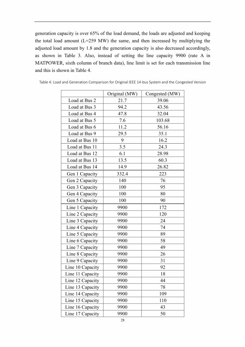
generation capacity is over 65% of the load demand, the loads are adjusted and keeping
the total load amount (L=259 MW) the same, and then increased by multiplying the
adjusted load amount by 1.8 and the generation capacity is also decreased accordingly,
as shown in Table 3. Also, instead of setting the line capacity 9900 (rate A in
MATPOWER, sixth column of branch data), line limit is set for each transmission line
and this is shown in Table 4.
Table 4: Load and Generation Comparison for Original IEEE 14‐bus System and the Congested Version
Original (MW) Congested (MW) Load at Bus 2 21.7 39.06 Load at Bus 3 94.2 43.56 Load at Bus 4 47.8 32.04 Load at Bus 5 7.6 103.68 Load at Bus 6 11.2 56.16 Load at Bus 9 29.5 35.1 Load at Bus 10 9 16.2 Load at Bus 11 3.5 24.3 Load at Bus 12 6.1 28.98 Load at Bus 13 13.5 60.3 Load at Bus 14 14.9 26.82
Gen 1 Capacity 332.4 223 Gen 2 Capacity 140 76 Gen 3 Capacity 100 95 Gen 4 Capacity 100 80 Gen 5 Capacity 100 90
Line 1 Capacity 9900 172 Line 2 Capacity 9900 120 Line 3 Capacity 9900 24 Line 4 Capacity 9900 74 Line 5 Capacity 9900 89 Line 6 Capacity 9900 58 Line 7 Capacity 9900 49 Line 8 Capacity 9900 26 Line 9 Capacity 9900 31
Line 10 Capacity 9900 92 Line 11 Capacity 9900 18 Line 12 Capacity 9900 44 Line 13 Capacity 9900 78 Line 14 Capacity 9900 109 Line 15 Capacity 9900 110 Line 16 Capacity 9900 43 Line 17 Capacity 9900 50
29
Line 18 Capacity 9900 25 Line 19 Capacity 9900 6 Line 20 Capacity 9900 14
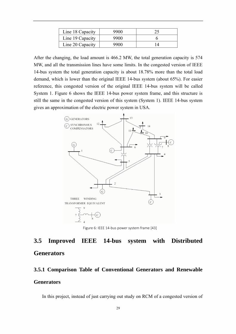
After the changing, the load amount is 466.2 MW, the total generation capacity is 574
MW, and all the transmission lines have some limits. In the congested version of IEEE
14-bus system the total generation capacity is about 18.78% more than the total load
demand, which is lower than the original IEEE 14-bus system (about 65%). For easier
reference, this congested version of the original IEEE 14-bus system will be called
System 1. Figure 6 shows the IEEE 14-bus power system frame, and this structure is
still the same in the congested version of this system (System 1). IEEE 14-bus system
gives an approximation of the electric power system in USA.
3.5 Improved IEEE 14-bus system with Distributed
Generators
3.5.1 Comparison Table of Conventional Generators and Renewable
Generators
In this project, instead of just carrying out study on RCM of a congested version of
Figure 6: IEEE 14‐bus power system frame [43]
30
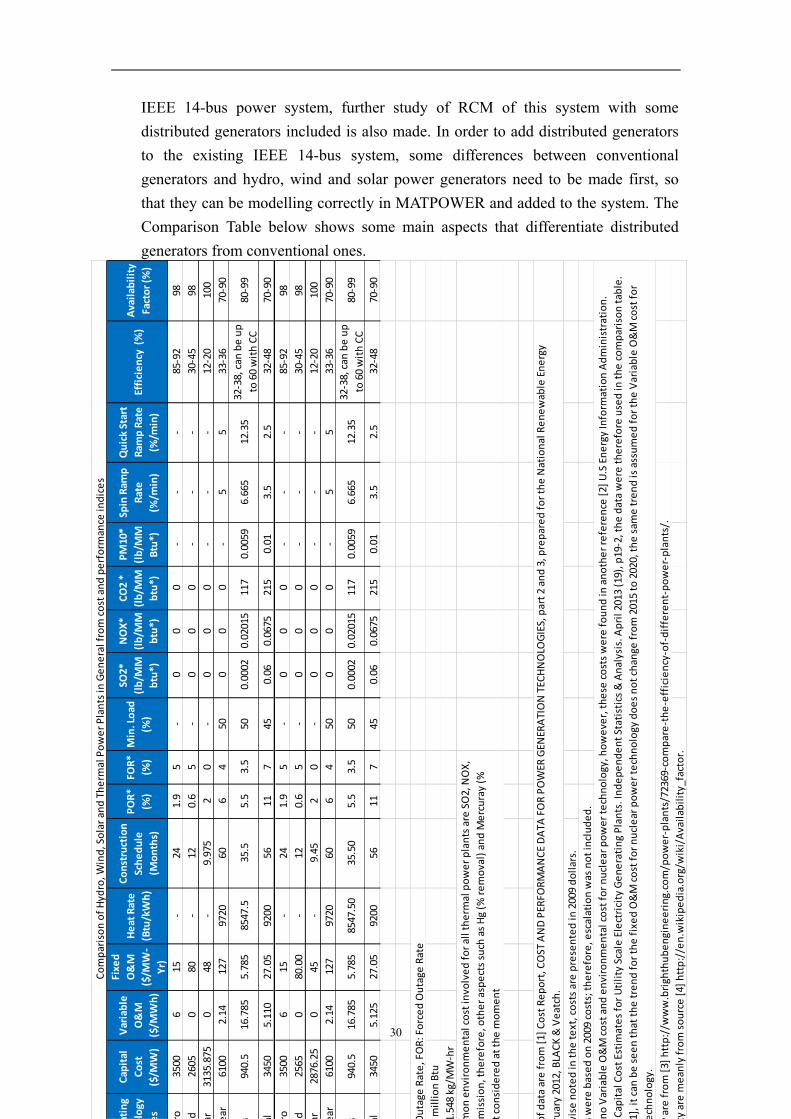
IEEE 14-bus power system, further study of RCM of this system with some
distributed generators included is also made. In order to add distributed generators
to the existing IEEE 14-bus system, some differences between conventional
generators and hydro, wind and solar power generators need to be made first, so
that they can be modelling correctly in MATPOWER and added to the system. The
Comparison Table below shows some main aspects that differentiate distributed
generators from conventional ones.
ating
ology
es
Capital
Cost
($/M
W)
Variable
O&M
($/M
Wh)
Fixed
O&M
($/M
W‐
Yr)
Heat Rate
(Btu/kWh)
Construction
Schedule
(Months)
POR*
(%)
FOR*
(%)
Min. Load
(%)
SO2*
(lb/M
M
btu*)
NOX*
(lb/M
M
btu*)
CO2 *
(lb/M
M
btu*)
PM10*
(lb/M
M
Btu*)
Spin Ram
p
Rate
(%/m
in)
Quick Start
Ram
p Rate
(%/m
in)
Efficiency (%)
Availability
Factor (%
)
ro3500
615
‐24
1.9
5‐
00
0‐
‐‐
85‐92
98
d2605
080
‐12
0.6
5‐
00
0‐
‐‐
30‐45
98
ar3135.875
048
‐9.975
20
‐0
00
‐‐
‐12‐20
100
ear
6100
2.14
127
9720
606
450
00
0‐
55
33‐36
70‐90
s 940.5
16.785
5.785
8547.5
35.5
5.5
3.5
500.0002
0.02015
117
0.0059
6.665
12.35
32‐38, can
be up
to 60 with CC
80‐99
al3450
5.110
27.05
9200
5611
745
0.06
0.0675
215
0.01
3.5
2.5
32‐48
70‐90
ro3500
615
‐24
1.9
5‐
00
0‐
‐‐
85‐92
98
d2565
080.00
‐12
0.6
5‐
00
0‐
‐‐
30‐45
98
ar2876.25
045
‐9.45
20
‐0
00
‐‐
‐12‐20
100
ear
6100
2.14
127
9720
606
450
00
0‐
55
33‐36
70‐90
s 940.5
16.785
5.785
8547.50
35.50
5.5
3.5
500.0002
0.02015
117
0.0059
6.665
12.35
32‐38, can
be up
to 60 with CC
80‐99
al3450
5.125
27.05
9200
5611
745
0.06
0.0675
215
0.01
3.5
2.5
32‐48
70‐90
Outage
Rate, FOR: Forced Outage
Rate
million Btu
wise noted in
the text, costs are presented in
2009 dollars.
s were based on 2009 costs; therefore, escalation was not included.
y are from [3] http://w
ww.brighthubengineering.com/power‐plants/72369‐compare‐the‐efficiency‐of‐different‐power‐plants/.
ty are meanly from source [4] http://en.wikipedia.org/w
iki/Availability_factor.
mon environmental cost involved for all therm
al power plants are SO2, NOX,
mission, therefore, other aspects such as Hg (%
removal) and Mercuray (%
t considered at the moment
Comparison of Hydro, W
ind, Solar and Therm
al Power Plants in
General from cost and perform
ance indices
of data are from [1] Cost Report, COST AND PERFO
RMANCE DATA
FOR POWER
GEN
ERATION TECHNOLO
GIES, part 2 and 3, prepared for the National Renewable Energy
ruary 2012, BLACK & Veatch.
1.548 kg/M
W‐hr
no Variable O&M cost and environmental cost for nuclear power technology, however, these costs were found in
another reference [2] U.S Energy Inform
ation Administration.
Capital Cost Estim
ates for Utility Scale Electricity Generating Plants. Independent Statistics & Analysis. A
pril 2013 (19), p19‐2, the data were therefore used in
the comparison table.
1], it can be seen that the trend for the fixed O&M cost for nuclear power technology does not change
from 2015 to 2020, the sam
e trend is assumed for the Variable O&M cost for
echnology.
31
Based on data from [31] (Cost Report) in the Comparison Table above, several
aspects including Capital Cost, Variable O&M, different types of gas emission
amount and so on are compared for hydro power, wind power, solar, nuclear and
conventional generating technology (gas and coal) in year 2015 and the future trend
in 2020.
From the Comparison Table, it can be seen that solar, wind and hydro normally
have a relatively lower value of variable O&M. Also, the availability of those three
types of generating technologies are higher than the conventional generators. In this
project, Fixed O&M, Variable O&M, CO2 emission amount and Availability are
used to differentiate the renewable generators from those conventional ones and
they are used to model distributed generator in MATPOWER
3.5.2 Connecting voltage and capacity of distributed generators (solar,
wind and hydro)
In this project, both the system with and without distributed generators are
considered for Reliability Centred Maintenance, therefore, it is important to know
the major difference between conventional generators and distributed generators, so
that the reasonable modelling of distributed generators can be made and added to
the system.
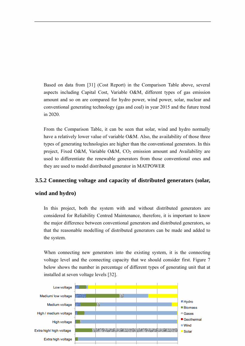
When connecting new generators into the existing system, it is the connecting
voltage level and the connecting capacity that we should consider first. Figure 7
below shows the number in percentage of different types of generating unit that at
installed at seven voltage levels [32].
32
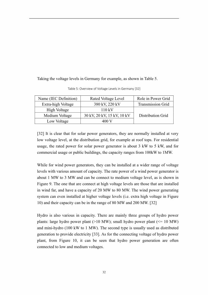
Taking the voltage levels in Germany for example, as shown in Table 5.
Table 5: Overview of Voltage Levels in Germany [32]
Name (IEC Definition) Rated Voltage Level Role in Power Grid Extra-high Voltage 380 kV, 220 kV Transmission Grid
High Voltage 110 kV Distribution Grid Medium Voltage 30 kV, 20 kV, 15 kV, 10 kV
Low Voltage 400 V
[32] It is clear that for solar power generators, they are normally installed at very
low voltage level, at the distribution grid, for example at roof tops. For residential
usage, the rated power for solar power generator is about 3 kW to 5 kW, and for
commercial usage or public buildings, the capacity ranges from 100kW to 1MW.
While for wind power generators, they can be installed at a wider range of voltage
levels with various amount of capacity. The rate power of a wind power generator is
about 1 MW to 3 MW and can be connect to medium voltage level, as is shown in
Figure 9. The one that are connect at high voltage levels are those that are installed
in wind far, and have a capacity of 20 MW to 80 MW. The wind power generating
system can even installed at higher voltage levels (i.e. extra high voltage in Figure
10) and their capacity can be in the range of 80 MW and 200 MW. [32]
Hydro is also various in capacity. There are mainly three groups of hydro power
plants: large hydro power plant (>10 MW); small hydro power plant (<= 10 MW)
and mini-hydro (100 kW to 1 MW). The second type is usually used as distributed
generation to provide electricity [33]. As for the connecting voltage of hydro power
plant, from Figure 10, it can be seen that hydro power generation are often
connected to low and medium voltages.
33
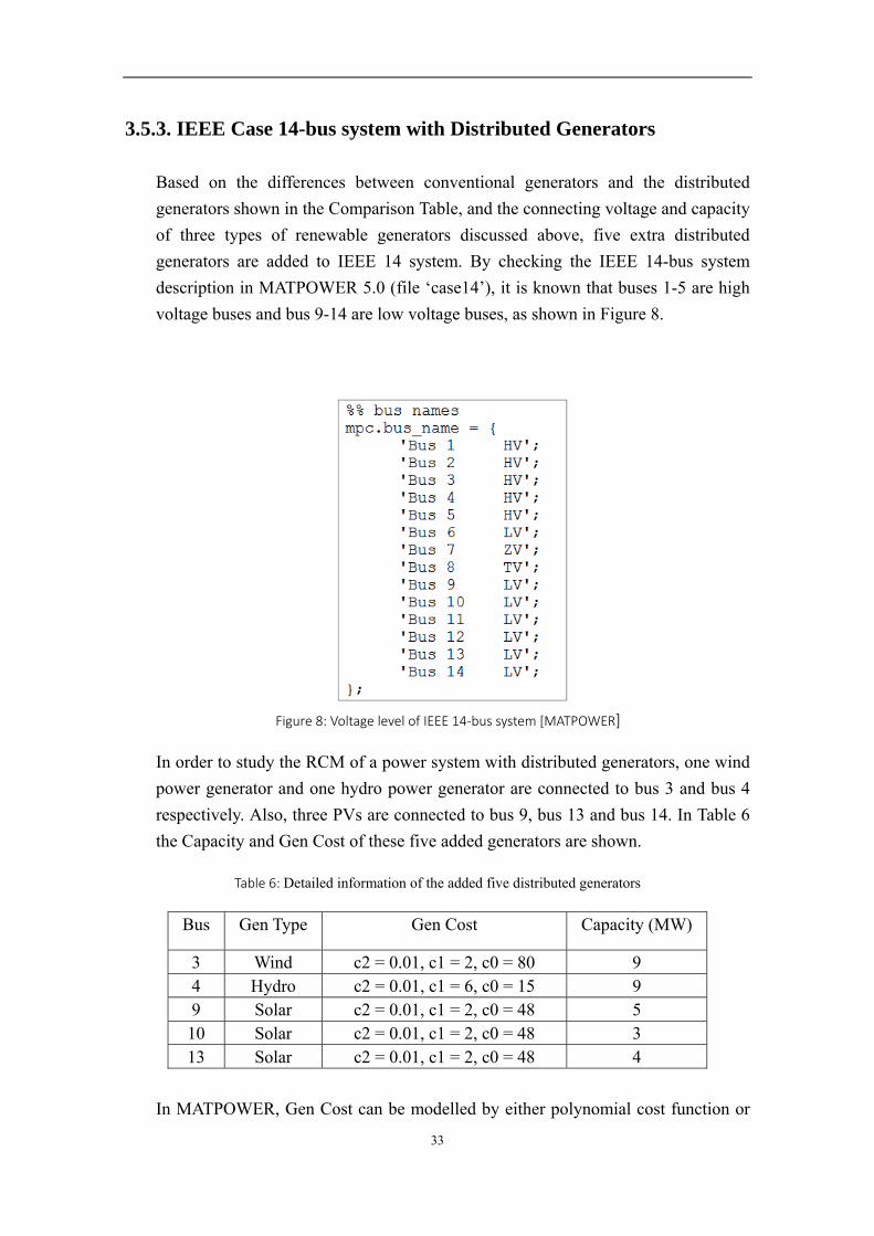
3.5.3. IEEE Case 14-bus system with Distributed Generators
Based on the differences between conventional generators and the distributed
generators shown in the Comparison Table, and the connecting voltage and capacity
of three types of renewable generators discussed above, five extra distributed
generators are added to IEEE 14 system. By checking the IEEE 14-bus system
description in MATPOWER 5.0 (file ‘case14’), it is known that buses 1-5 are high
voltage buses and bus 9-14 are low voltage buses, as shown in Figure 8.
In order to study the RCM of a power system with distributed generators, one wind
power generator and one hydro power generator are connected to bus 3 and bus 4
respectively. Also, three PVs are connected to bus 9, bus 13 and bus 14. In Table 6
the Capacity and Gen Cost of these five added generators are shown.
Table 6: Detailed information of the added five distributed generators
Bus Gen Type Gen Cost Capacity (MW)
3 Wind c2 = 0.01, c1 = 2, c0 = 80 9 4 Hydro c2 = 0.01, c1 = 6, c0 = 15 9 9 Solar c2 = 0.01, c1 = 2, c0 = 48 5 10 Solar c2 = 0.01, c1 = 2, c0 = 48 3 13 Solar c2 = 0.01, c1 = 2, c0 = 48 4
In MATPOWER, Gen Cost can be modelled by either polynomial cost function or
Figure 8: Voltage level of IEEE 14‐bus system [MATPOWER]
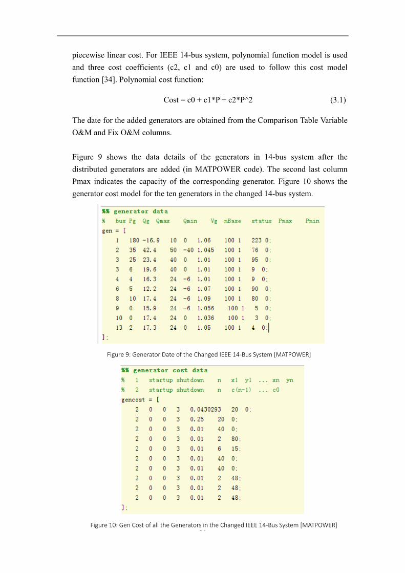
34
piecewise linear cost. For IEEE 14-bus system, polynomial function model is used
and three cost coefficients (c2, c1 and c0) are used to follow this cost model
function [34]. Polynomial cost function:
Cost = c0 + c1*P + c2*P^2 (3.1)
The date for the added generators are obtained from the Comparison Table Variable
O&M and Fix O&M columns.
Figure 9 shows the data details of the generators in 14-bus system after the
distributed generators are added (in MATPOWER code). The second last column
Pmax indicates the capacity of the corresponding generator. Figure 10 shows the
generator cost model for the ten generators in the changed 14-bus system.
Figure 10: Gen Cost of all the Generators in the Changed IEEE 14‐Bus System [MATPOWER]
Figure 9: Generator Date of the Changed IEEE 14‐Bus System [MATPOWER]

35
For easier reference, this system with distributed generator will be called System 2.
The RCM is first studied on the more congested version of IEEE 14-bus system and
then on the system that has the distributed generators added. In the next part,
detailed description of the different contingencies considered in the project is given.
Since RCM depends on probability to some extent, for example, probability of the
availability of generators and transmission lines, it is important to understand what
kinds of contingencies are calculated to obtain the average value of ENS, Operating
& Interruption Cost, Environmental Cost, etc.
3.6 Other Calculations
3.6.1 EENS Calculating Model
As explained in 2.2, EENS means Energy Not Supplied. In this project, in order to
obtain the energy not supplied for each contingency, in creating the system for
RCM study, some virtual generators are connected to both the congested version of
IEEE 14-bus (System 1) and also the system with distributed generators added
(System 2) explained more in details in 3.3 and 3.4. The generation amount from
these virtual generators can represent ENS of each contingency and the
corresponding cost reveals the interruption cost.
These virtual generators are connected to the buses to which load is connected to
guarantee that the system still converges when one or two components (generator or
line) go to outage and ENS of each contingency can be obtained in a relatively easy
way. In the IEEE 14-bus power system, loads are connected to bus 2-6 and bus 9-14,
which can be seen in Table 3. The capacity of these virtual generators equal to the
load amount at the bus that they are connected to. The generation from these virtual
generators can be viewed as the energy not supplied, they are assigned a high value
of € 5970/MWh [35] ($ 6752/MWh) for c1 in their Gen Cost function to represent
the Value of Loss Load (VOLL). In order to only let virtual generators to produce
electricity unless necessary, the c2 of virtual generators is assigned as the highest c2
among all the real generators, which is 0.25. Table 7 shows the data for these added
virtual generators.
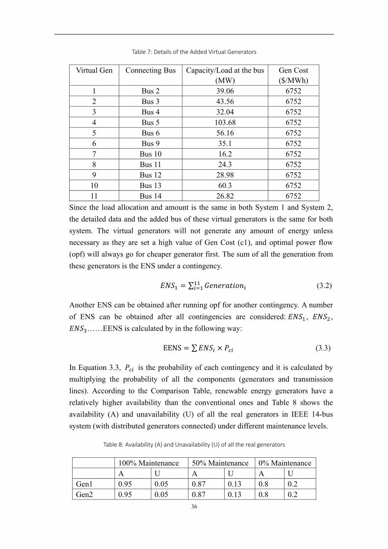
36
Table 7: Details of the Added Virtual Generators
Virtual Gen Connecting Bus Capacity/Load at the bus (MW)
Gen Cost ($/MWh)
1 Bus 2 39.06 6752 2 Bus 3 43.56 6752 3 Bus 4 32.04 6752 4 Bus 5 103.68 6752 5 Bus 6 56.16 6752 6 Bus 9 35.1 6752 7 Bus 10 16.2 6752 8 Bus 11 24.3 6752 9 Bus 12 28.98 6752 10 Bus 13 60.3 6752 11 Bus 14 26.82 6752
Since the load allocation and amount is the same in both System 1 and System 2,
the detailed data and the added bus of these virtual generators is the same for both
system. The virtual generators will not generate any amount of energy unless
necessary as they are set a high value of Gen Cost (c1), and optimal power flow
(opf) will always go for cheaper generator first. The sum of all the generation from
these generators is the ENS under a contingency.
∑ (3.2)
Another ENS can be obtained after running opf for another contingency. A number
of ENS can be obtained after all contingencies are considered: , ,
……EENS is calculated by in the following way:
EENS ∑ (3.3)
In Equation 3.3, is the probability of each contingency and it is calculated by
multiplying the probability of all the components (generators and transmission
lines). According to the Comparison Table, renewable energy generators have a
relatively higher availability than the conventional ones and Table 8 shows the
availability (A) and unavailability (U) of all the real generators in IEEE 14-bus
system (with distributed generators connected) under different maintenance levels.
Table 8: Availability (A) and Unavailability (U) of all the real generators
100% Maintenance 50% Maintenance 0% Maintenance A U A U A U Gen1 0.95 0.05 0.87 0.13 0.8 0.2 Gen2 0.95 0.05 0.87 0.13 0.8 0.2
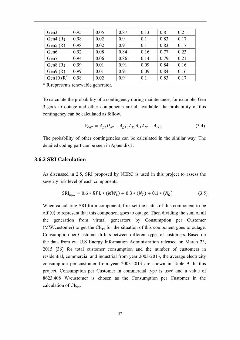
37
Gen3 0.95 0.05 0.87 0.13 0.8 0.2 Gen4 (R) 0.98 0.02 0.9 0.1 0.83 0.17 Gen5 (R) 0.98 0.02 0.9 0.1 0.83 0.17 Gen6 0.92 0.08 0.84 0.16 0.77 0.23 Gen7 0.94 0.06 0.86 0.14 0.79 0.21 Gen8 (R) 0.99 0.01 0.91 0.09 0.84 0.16 Gen9 (R) 0.99 0.01 0.91 0.09 0.84 0.16 Gen10 (R) 0.98 0.02 0.9 0.1 0.83 0.17
* R represents renewable generator.
To calculate the probability of a contingency during maintenance, for example, Gen
3 goes to outage and other components are all available, the probability of this
contingency can be calculated as follow.
P … … (3.4)
The probability of other contingencies can be calculated in the similar way. The
detailed coding part can be seen in Appendix I.
3.6.2 SRI Calculation
As discussed in 2.5, SRI proposed by NERC is used in this project to assess the
severity risk level of each components.
SRI 0.6 ∗ ∗ 0.3 ∗ 0.1 ∗ (3.5)
When calculating SRI for a component, first set the status of this component to be
off (0) to represent that this component goes to outage. Then dividing the sum of all
the generation from virtual generators by Consumption per Customer
(MW/customer) to get the CIbps for the situation of this component goes to outage.
Consumption per Customer differs between different types of customers. Based on
the data from eia U.S Energy Information Administration released on March 23,
2015 [36] for total customer consumption and the number of customers in
residential, commercial and industrial from year 2003-2013, the average electricity
consumption per customer from year 2003-2013 are shown in Table 9. In this
project, Consumption per Customer in commercial type is used and a value of
8623.408 W/customer is chosen as the Consumption per Customer in the
calculation of CIbps.
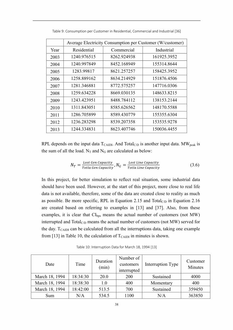
38
Table 9: Consumption per Customer in Residential, Commercial and Industrial [36]
Average Electricity Consumption per Customer (W/customer)
Year Residential Commercial Industrial
2003 1240.976515 8262.924938 161925.3952
2004 1240.997849 8452.168949 155314.8644
2005 1283.99817 8621.257257 158425.3952
2006 1258.889162 8634.214929 151876.4506
2007 1281.346881 8772.575257 147716.0306
2008 1259.634228 8669.030135 148633.8215
2009 1243.423951 8488.784112 138153.2144
2010 1311.843051 8585.626562 148170.5588
2011 1286.705899 8589.430779 155355.6304
2012 1236.283298 8539.207358 153535.9278
2013 1244.334831 8623.407746 150036.4455
RPL depends on the input data TCAIDI. And TotalC/D is another input data. MWpeak is
the sum of all the load. NT and NG are calculated as below:
,
(3.6)
In this project, for better simulation to reflect real situation, some industrial data
should have been used. However, at the start of this project, more close to real life
data is not available, therefore, some of the data are created close to reality as much
as possible. Be more specific, RPL in Equation 2.15 and TotalC/D in Equation 2.16
are created based on referring to examples in [13] and [37]. Also, from these
examples, it is clear that CIbps means the actual number of customers (not MW)
interrupted and TotalC/D means the actual number of customers (not MW) served for
the day. TCAIDI can be calculated from all the interruptions data, taking one example
from [13] in Table 10, the calculation of TCAIDI in minutes is shown.
Table 10: Interruption Data for March 18, 1994 [13]
Date Time Duration
(min)
Number of customers interrupted
Interruption Type Customer Minutes
March 18, 1994 18:34:30 20.0 200 Sustained 4000 March 18, 1994 18:38:30 1.0 400 Momentary 400 March 18, 1994 18:42:00 513.5 700 Sustained 359450
Sum N/A 534.5 1100 N/A 363850
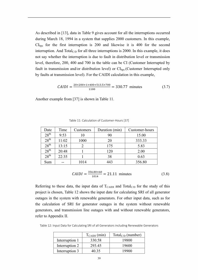
39
As described in [13], data in Table 9 gives account for all the interruptions occurred
during March 18, 1994 in a system that supplies 2000 customers. In this example,
CIbps for the first interruption is 200 and likewise it is 400 for the second
interruption. And TotalC/D for all three interruptions is 2000. In this example, it does
not say whether the interruption is due to fault in distribution level or transmission
level, therefore, 200, 400 and 700 in the table can be CI (Customer Interrupted by
fault in transmission and/or distribution level) or CIbps (Customer Interrupted only
by faults at transmission level). For the CAIDI calculation in this example,
. 330.77 minutes (3.7)
Another example from [37] is shown in Table 11.
Table 11: Calculation of Customer‐Hours [37]
Date Time Customers Duration (min) Customer-hours 28th 9:53 10 90 15.00 28th 11:02 1000 20 333.33 28th 13:15 2 175 5.83 28th 20:48 1 120 2.00 28th 22:35 1 38 0.63 Sum -- 1014 443 356.80
. 21.11 minutes (3.8)
Referring to these data, the input data of TCAIDI and TotalC/D for the study of this
project is chosen, Table 12 shows the input date for calculating SRI of all generator
outages in the system with renewable generators. For other input data, such as for
the calculation of SRI for generator outages in the system without renewable
generators, and transmission line outages with and without renewable generators,
refer to Appendix II.
Table 12: Input Data for Calculating SRI of all Generators including Renewable Generators
TCAIDI (min) TotalC/D (number) Interruption 1 330.58 19800 Interruption 2 293.45 19600 Interruption 3 40.35 19900
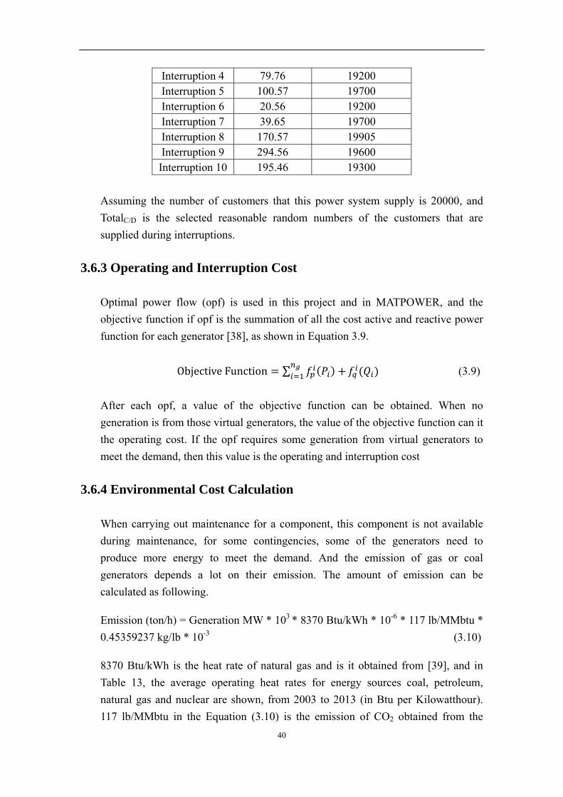
40
Interruption 4 79.76 19200 Interruption 5 100.57 19700 Interruption 6 20.56 19200 Interruption 7 39.65 19700 Interruption 8 170.57 19905 Interruption 9 294.56 19600 Interruption 10 195.46 19300
Assuming the number of customers that this power system supply is 20000, and
TotalC/D is the selected reasonable random numbers of the customers that are
supplied during interruptions.
3.6.3 Operating and Interruption Cost
Optimal power flow (opf) is used in this project and in MATPOWER, and the
objective function if opf is the summation of all the cost active and reactive power
function for each generator [38], as shown in Equation 3.9.
ObjectiveFunction ∑ (3.9)
After each opf, a value of the objective function can be obtained. When no
generation is from those virtual generators, the value of the objective function can it
the operating cost. If the opf requires some generation from virtual generators to
meet the demand, then this value is the operating and interruption cost
3.6.4 Environmental Cost Calculation
When carrying out maintenance for a component, this component is not available
during maintenance, for some contingencies, some of the generators need to
produce more energy to meet the demand. And the emission of gas or coal
generators depends a lot on their emission. The amount of emission can be
calculated as following.
Emission (ton/h) = Generation MW * 103 * 8370 Btu/kWh * 10-6 * 117 lb/MMbtu *
0.45359237 kg/lb * 10-3 (3.10)
8370 Btu/kWh is the heat rate of natural gas and is it obtained from [39], and in
Table 13, the average operating heat rates for energy sources coal, petroleum,
natural gas and nuclear are shown, from 2003 to 2013 (in Btu per Kilowatthour).
117 lb/MMbtu in the Equation (3.10) is the emission of CO2 obtained from the
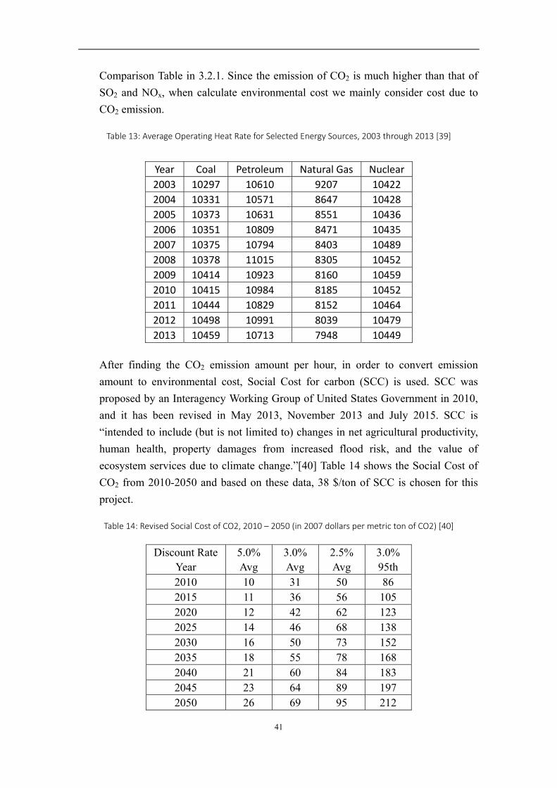
41
Comparison Table in 3.2.1. Since the emission of CO2 is much higher than that of
SO2 and NOx, when calculate environmental cost we mainly consider cost due to
CO2 emission.
Table 13: Average Operating Heat Rate for Selected Energy Sources, 2003 through 2013 [39]
After finding the CO2 emission amount per hour, in order to convert emission
amount to environmental cost, Social Cost for carbon (SCC) is used. SCC was
proposed by an Interagency Working Group of United States Government in 2010,
and it has been revised in May 2013, November 2013 and July 2015. SCC is
“intended to include (but is not limited to) changes in net agricultural productivity,
human health, property damages from increased flood risk, and the value of
ecosystem services due to climate change.”[40] Table 14 shows the Social Cost of
CO2 from 2010-2050 and based on these data, 38 $/ton of SCC is chosen for this
project.
Table 14: Revised Social Cost of CO2, 2010 – 2050 (in 2007 dollars per metric ton of CO2) [40]
Discount Rate Year
5.0% Avg
3.0% Avg
2.5% Avg
3.0% 95th
2010 10 31 50 86 2015 11 36 56 105 2020 12 42 62 123 2025 14 46 68 138 2030 16 50 73 152 2035 18 55 78 168 2040 21 60 84 183 2045 23 64 89 197 2050 26 69 95 212
Year Coal Petroleum Natural Gas Nuclear
2003 10297 10610 9207 10422
2004 10331 10571 8647 10428
2005 10373 10631 8551 10436
2006 10351 10809 8471 10435
2007 10375 10794 8403 10489
2008 10378 11015 8305 10452
2009 10414 10923 8160 10459
2010 10415 10984 8185 10452
2011 10444 10829 8152 10464
2012 10498 10991 8039 10479
2013 10459 10713 7948 10449
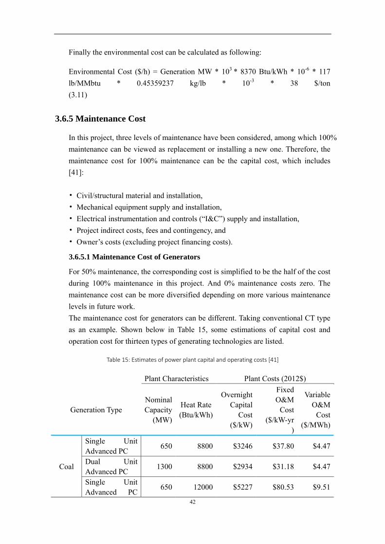
42
Finally the environmental cost can be calculated as following:
Environmental Cost ($/h) = Generation MW * 103 * 8370 Btu/kWh * 10-6 * 117
lb/MMbtu * 0.45359237 kg/lb * 10-3 * 38 $/ton
(3.11)
3.6.5 Maintenance Cost
In this project, three levels of maintenance have been considered, among which 100%
maintenance can be viewed as replacement or installing a new one. Therefore, the
maintenance cost for 100% maintenance can be the capital cost, which includes
[41]:
• Civil/structural material and installation,
• Mechanical equipment supply and installation,
• Electrical instrumentation and controls (“I&C”) supply and installation,
• Project indirect costs, fees and contingency, and
• Owner’s costs (excluding project financing costs).
3.6.5.1 Maintenance Cost of Generators
For 50% maintenance, the corresponding cost is simplified to be the half of the cost
during 100% maintenance in this project. And 0% maintenance costs zero. The
maintenance cost can be more diversified depending on more various maintenance
levels in future work.
The maintenance cost for generators can be different. Taking conventional CT type
as an example. Shown below in Table 15, some estimations of capital cost and
operation cost for thirteen types of generating technologies are listed.
Table 15: Estimates of power plant capital and operating costs [41]
Plant Characteristics Plant Costs (2012$)
Generation Type Nominal Capacity
(MW)
Heat Rate (Btu/kWh)
Overnight Capital
Cost ($/kW)
Fixed O&M
Cost ($/kW-yr
)
Variable O&M
Cost ($/MWh)
Coal
Single Unit Advanced PC
650 8800 $3246 $37.80 $4.47
Dual Unit Advanced PC
1300 8800 $2934 $31.18 $4.47
Single Unit Advanced PC
650 12000 $5227 $80.53 $9.51
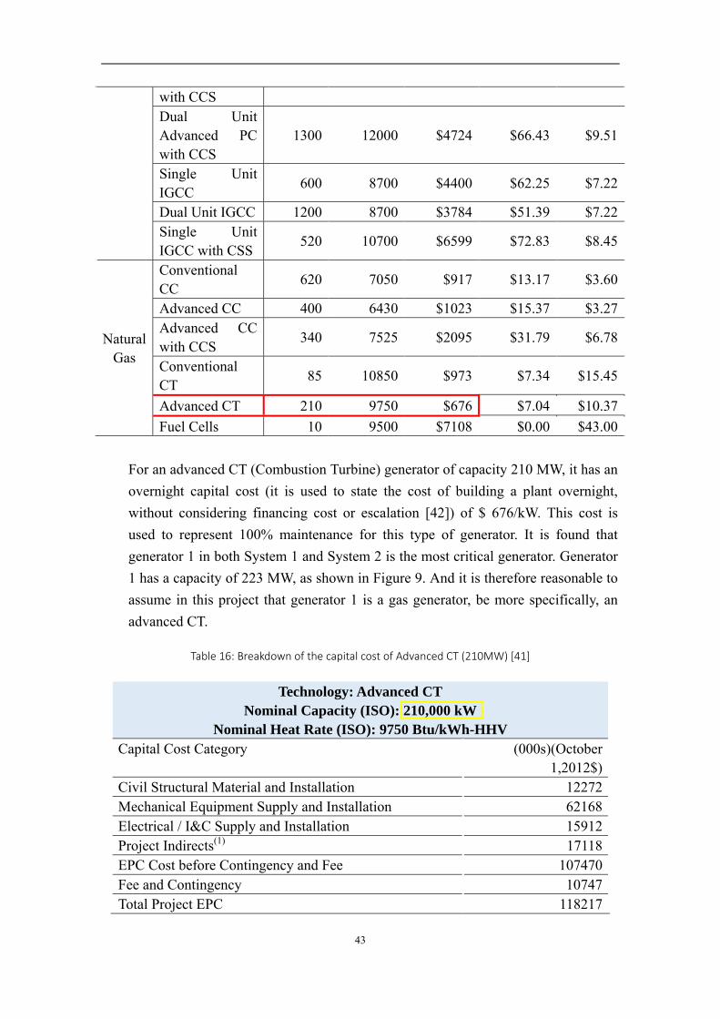
43
with CCS Dual Unit Advanced PC with CCS
1300 12000 $4724 $66.43 $9.51
Single Unit IGCC
600 8700 $4400 $62.25 $7.22
Dual Unit IGCC 1200 8700 $3784 $51.39 $7.22 Single Unit IGCC with CSS
520 10700 $6599 $72.83 $8.45
Natural Gas
Conventional CC
620 7050 $917 $13.17 $3.60
Advanced CC 400 6430 $1023 $15.37 $3.27 Advanced CC with CCS
340 7525 $2095 $31.79 $6.78
Conventional CT
85 10850 $973 $7.34 $15.45
Advanced CT 210 9750 $676 $7.04 $10.37
Fuel Cells 10 9500 $7108 $0.00 $43.00
For an advanced CT (Combustion Turbine) generator of capacity 210 MW, it has an
overnight capital cost (it is used to state the cost of building a plant overnight,
without considering financing cost or escalation [42]) of $ 676/kW. This cost is
used to represent 100% maintenance for this type of generator. It is found that
generator 1 in both System 1 and System 2 is the most critical generator. Generator
1 has a capacity of 223 MW, as shown in Figure 9. And it is therefore reasonable to
assume in this project that generator 1 is a gas generator, be more specifically, an
advanced CT.
Table 16: Breakdown of the capital cost of Advanced CT (210MW) [41]
Technology: Advanced CT Nominal Capacity (ISO): 210,000 kW
Nominal Heat Rate (ISO): 9750 Btu/kWh-HHV Capital Cost Category (000s)(October
1,2012$) Civil Structural Material and Installation 12272 Mechanical Equipment Supply and Installation 62168 Electrical / I&C Supply and Installation 15912 Project Indirects(1) 17118 EPC Cost before Contingency and Fee 107470 Fee and Contingency 10747 Total Project EPC 118217
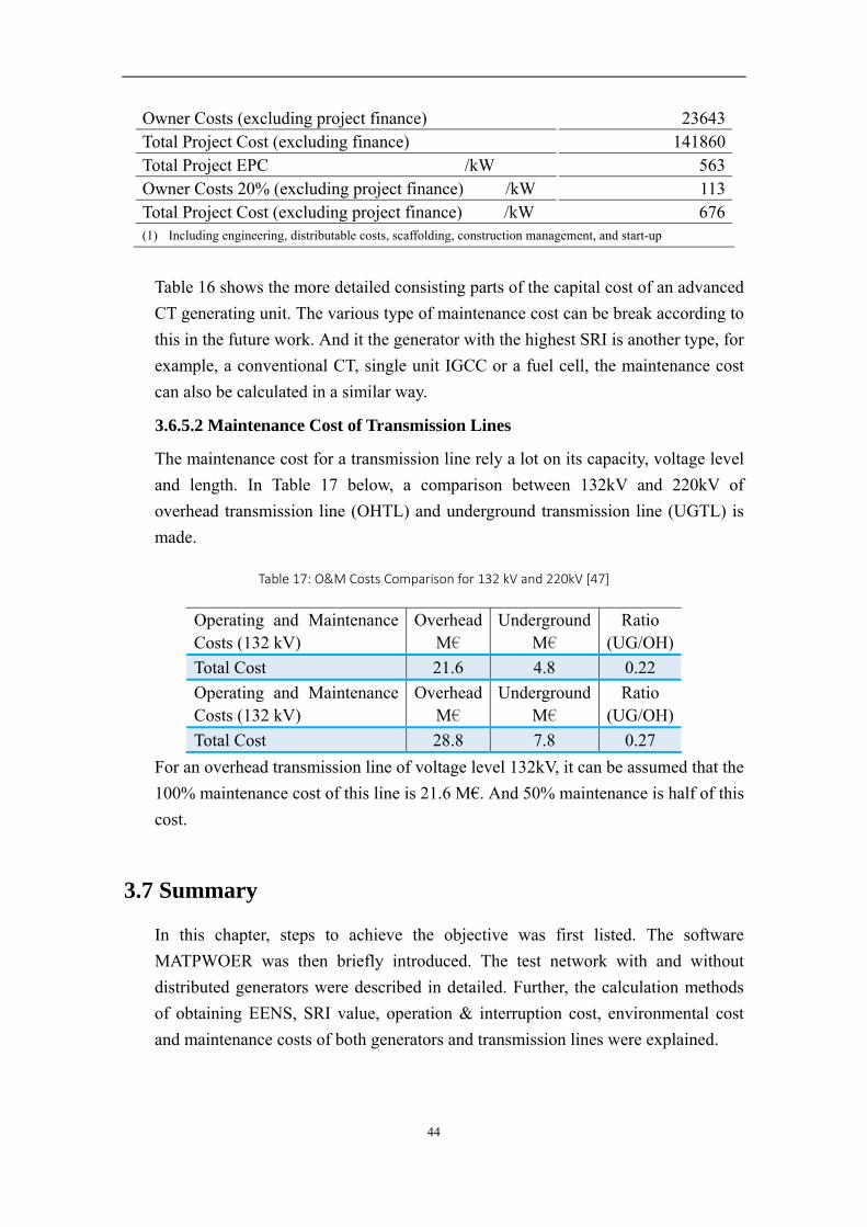
44
Owner Costs (excluding project finance) 23643 Total Project Cost (excluding finance) 141860 Total Project EPC /kW 563 Owner Costs 20% (excluding project finance) /kW 113 Total Project Cost (excluding project finance) /kW 676 (1) Including engineering, distributable costs, scaffolding, construction management, and start-up
Table 16 shows the more detailed consisting parts of the capital cost of an advanced
CT generating unit. The various type of maintenance cost can be break according to
this in the future work. And it the generator with the highest SRI is another type, for
example, a conventional CT, single unit IGCC or a fuel cell, the maintenance cost
can also be calculated in a similar way.
3.6.5.2 Maintenance Cost of Transmission Lines
The maintenance cost for a transmission line rely a lot on its capacity, voltage level
and length. In Table 17 below, a comparison between 132kV and 220kV of
overhead transmission line (OHTL) and underground transmission line (UGTL) is
made.
Table 17: O&M Costs Comparison for 132 kV and 220kV [47]
Operating and Maintenance Costs (132 kV)
Overhead M€
Underground M€
Ratio (UG/OH)
Total Cost 21.6 4.8 0.22
Operating and Maintenance Costs (132 kV)
Overhead M€
Underground M€
Ratio (UG/OH)
Total Cost 28.8 7.8 0.27
For an overhead transmission line of voltage level 132kV, it can be assumed that the
100% maintenance cost of this line is 21.6 M€. And 50% maintenance is half of this
cost.
3.7 Summary
In this chapter, steps to achieve the objective was first listed. The software
MATPWOER was then briefly introduced. The test network with and without
distributed generators were described in detailed. Further, the calculation methods
of obtaining EENS, SRI value, operation & interruption cost, environmental cost
and maintenance costs of both generators and transmission lines were explained.
45
Chapter 4
Simulation Results and Discussion
This chapter presents all the obtained results. Firstly, simulation results for both IEEE 14-bus system with and without renewable energy generator, which is the Base Case, are shown and compared. Then, results for two sensitivity study cases are simulated and shown. In Case 1, the capacity of the added renewable energy generators is increased and in Case 2 the capacity of the transmission line is increased.
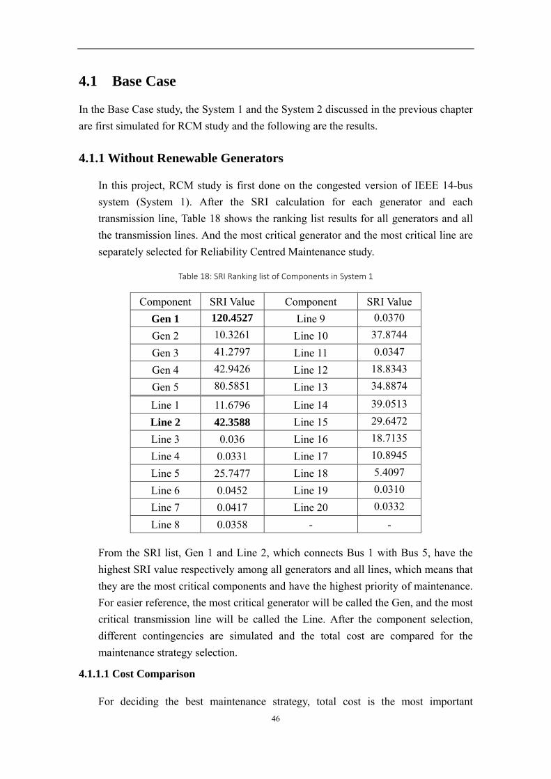
46
4.1 Base Case
In the Base Case study, the System 1 and the System 2 discussed in the previous chapter
are first simulated for RCM study and the following are the results.
4.1.1 Without Renewable Generators
In this project, RCM study is first done on the congested version of IEEE 14-bus
system (System 1). After the SRI calculation for each generator and each
transmission line, Table 18 shows the ranking list results for all generators and all
the transmission lines. And the most critical generator and the most critical line are
separately selected for Reliability Centred Maintenance study.
Table 18: SRI Ranking list of Components in System 1
Component SRI Value Component SRI Value
Gen 1 120.4527 Line 9 0.0370
Gen 2 10.3261 Line 10 37.8744
Gen 3 41.2797 Line 11 0.0347
Gen 4 42.9426 Line 12 18.8343
Gen 5 80.5851 Line 13 34.8874
Line 1 11.6796 Line 14 39.0513
Line 2 42.3588 Line 15 29.6472
Line 3 0.036 Line 16 18.7135
Line 4 0.0331 Line 17 10.8945
Line 5 25.7477 Line 18 5.4097
Line 6 0.0452 Line 19 0.0310
Line 7 0.0417 Line 20 0.0332
Line 8 0.0358 - -
From the SRI list, Gen 1 and Line 2, which connects Bus 1 with Bus 5, have the
highest SRI value respectively among all generators and all lines, which means that
they are the most critical components and have the highest priority of maintenance.
For easier reference, the most critical generator will be called the Gen, and the most
critical transmission line will be called the Line. After the component selection,
different contingencies are simulated and the total cost are compared for the
maintenance strategy selection.
4.1.1.1 Cost Comparison
For deciding the best maintenance strategy, total cost is the most important
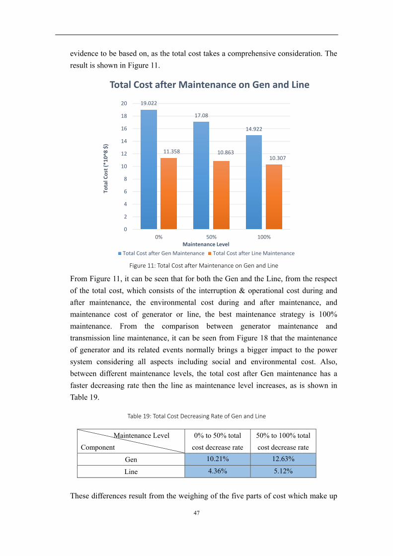
47
evidence to be based on, as the total cost takes a comprehensive consideration. The
result is shown in Figure 11.
From Figure 11, it can be seen that for both the Gen and the Line, from the respect
of the total cost, which consists of the interruption & operational cost during and
after maintenance, the environmental cost during and after maintenance, and
maintenance cost of generator or line, the best maintenance strategy is 100%
maintenance. From the comparison between generator maintenance and
transmission line maintenance, it can be seen from Figure 18 that the maintenance
of generator and its related events normally brings a bigger impact to the power
system considering all aspects including social and environmental cost. Also,
between different maintenance levels, the total cost after Gen maintenance has a
faster decreasing rate then the line as maintenance level increases, as is shown in
Table 19.
Table 19: Total Cost Decreasing Rate of Gen and Line
Maintenance Level
Component
0% to 50% total
cost decrease rate
50% to 100% total
cost decrease rate
Gen 10.21% 12.63%
Line 4.36% 5.12%
These differences result from the weighing of the five parts of cost which make up
Figure 11: Total Cost after Maintenance on Gen and Line
19.022
17.08
14.922
11.358 10.86310.307
0
2
4
6
8
10
12
14
16
18
20
0% 50% 100%
Total Cost (*10^8
$)
Maintenance Level
Total Cost after Maintenance on Gen and Line
Total Cost after Gen Maintenance Total Cost after Line Maintenance
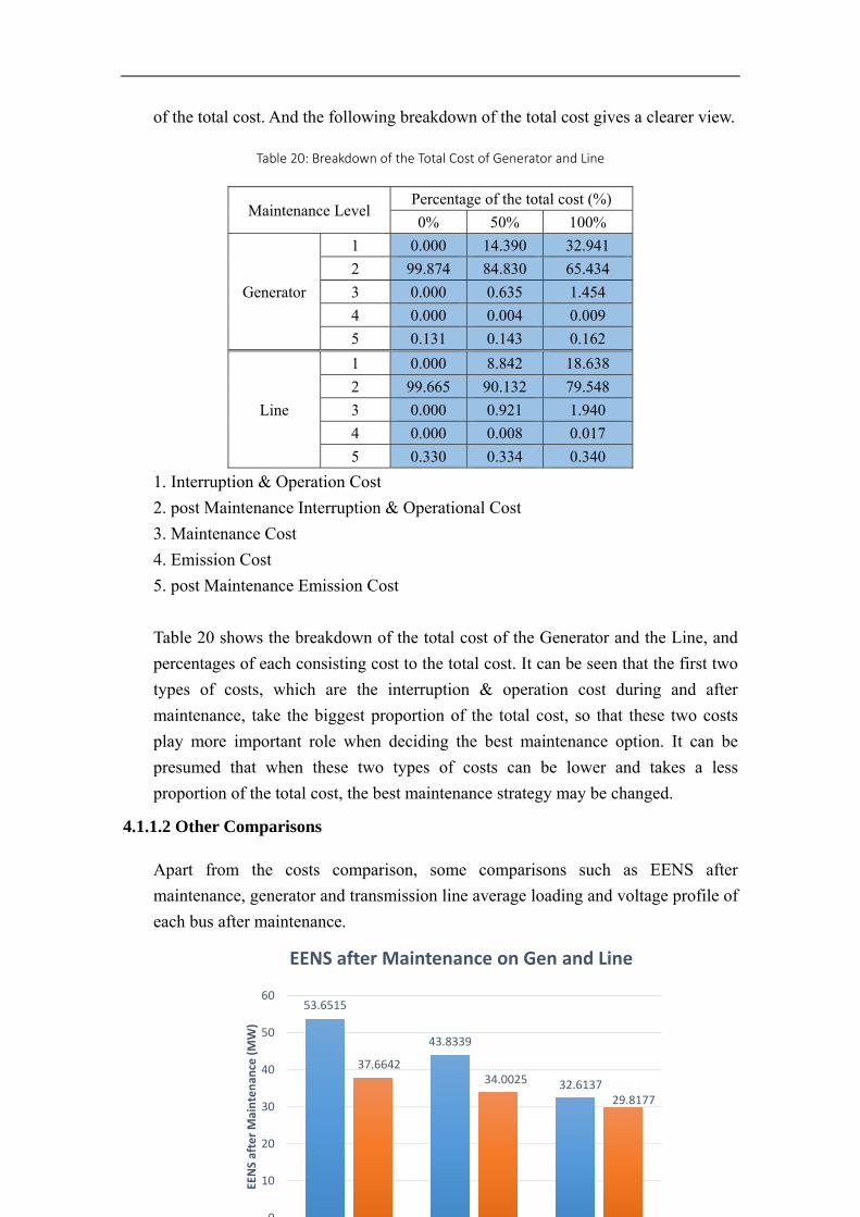
48
of the total cost. And the following breakdown of the total cost gives a clearer view.
Table 20: Breakdown of the Total Cost of Generator and Line
Maintenance Level Percentage of the total cost (%)
0% 50% 100%
Generator
1 0.000 14.390 32.941
2 99.874 84.830 65.434
3 0.000 0.635 1.454
4 0.000 0.004 0.009
5 0.131 0.143 0.162
Line
1 0.000 8.842 18.638
2 99.665 90.132 79.548
3 0.000 0.921 1.940
4 0.000 0.008 0.017
5 0.330 0.334 0.340
1. Interruption & Operation Cost
2. post Maintenance Interruption & Operational Cost
3. Maintenance Cost
4. Emission Cost
5. post Maintenance Emission Cost
Table 20 shows the breakdown of the total cost of the Generator and the Line, and
percentages of each consisting cost to the total cost. It can be seen that the first two
types of costs, which are the interruption & operation cost during and after
maintenance, take the biggest proportion of the total cost, so that these two costs
play more important role when deciding the best maintenance option. It can be
presumed that when these two types of costs can be lower and takes a less
proportion of the total cost, the best maintenance strategy may be changed.
4.1.1.2 Other Comparisons
Apart from the costs comparison, some comparisons such as EENS after
maintenance, generator and transmission line average loading and voltage profile of
each bus after maintenance.
53.6515
43.8339
32.6137
37.664234.0025
29.8177
0
10
20
30
40
50
60
EENS after Maintenan
ce (MW)
EENS after Maintenance on Gen and Line
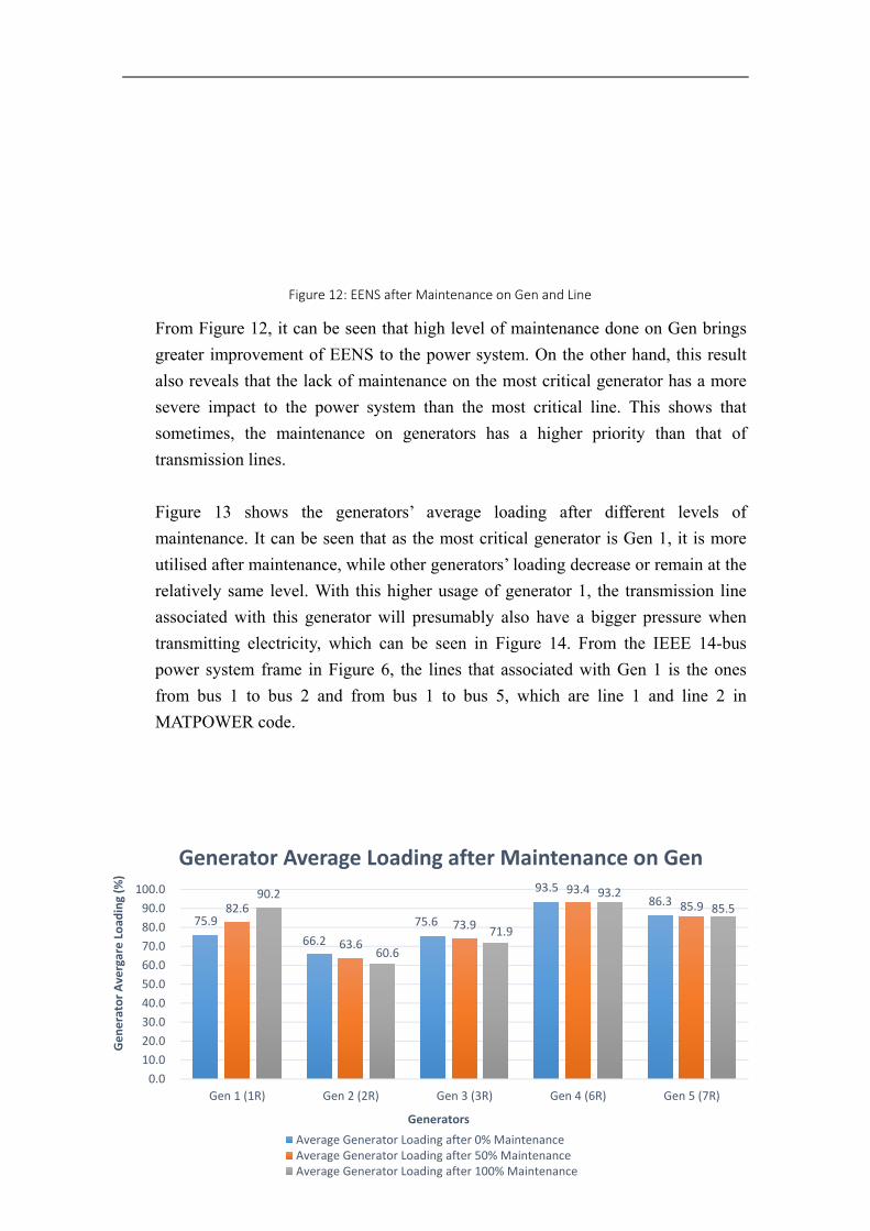
49
From Figure 12, it can be seen that high level of maintenance done on Gen brings
greater improvement of EENS to the power system. On the other hand, this result
also reveals that the lack of maintenance on the most critical generator has a more
severe impact to the power system than the most critical line. This shows that
sometimes, the maintenance on generators has a higher priority than that of
transmission lines.
Figure 13 shows the generators’ average loading after different levels of
maintenance. It can be seen that as the most critical generator is Gen 1, it is more
utilised after maintenance, while other generators’ loading decrease or remain at the
relatively same level. With this higher usage of generator 1, the transmission line
associated with this generator will presumably also have a bigger pressure when
transmitting electricity, which can be seen in Figure 14. From the IEEE 14-bus
power system frame in Figure 6, the lines that associated with Gen 1 is the ones
from bus 1 to bus 2 and from bus 1 to bus 5, which are line 1 and line 2 in
MATPOWER code.
Figure 12: EENS after Maintenance on Gen and Line
75.9
66.2
75.6
93.5 86.3
82.6
63.6
73.9
93.4
85.9 90.2
60.6
71.9
93.2 85.5
0.0
10.0
20.0
30.0
40.0
50.0
60.0
70.0
80.0
90.0
100.0
Gen 1 (1R) Gen 2 (2R) Gen 3 (3R) Gen 4 (6R) Gen 5 (7R)
Generator Avergare Load
ing (%
)
Generators
Generator Average Loading after Maintenance on Gen
Average Generator Loading after 0% MaintenanceAverage Generator Loading after 50% MaintenanceAverage Generator Loading after 100% Maintenance
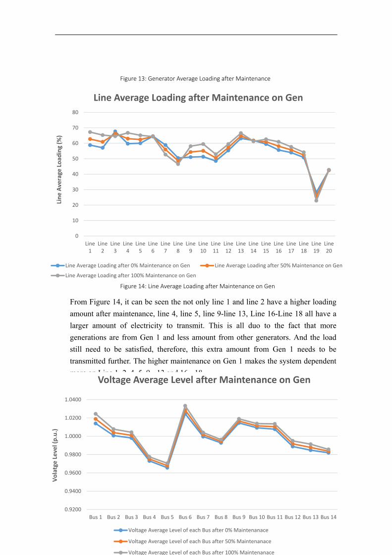
50
From Figure 14, it can be seen the not only line 1 and line 2 have a higher loading
amount after maintenance, line 4, line 5, line 9-line 13, Line 16-Line 18 all have a
larger amount of electricity to transmit. This is all duo to the fact that more
generations are from Gen 1 and less amount from other generators. And the load
still need to be satisfied, therefore, this extra amount from Gen 1 needs to be
transmitted further. The higher maintenance on Gen 1 makes the system dependent
more on Line 1, 2, 4, 5, 9 - 13 and 16 - 18
Figure 13: Generator Average Loading after Maintenance
0
10
20
30
40
50
60
70
80
Line1
Line2
Line3
Line4
Line5
Line6
Line7
Line8
Line9
Line10
Line11
Line12
Line13
Line14
Line15
Line16
Line17
Line18
Line19
Line20
Line Average
Load
ing (%
)
Line Average Loading after Maintenance on Gen
Line Average Loading after 0% Maintenance on Gen Line Average Loading after 50% Maintenance on Gen
Line Average Loading after 100% Maintenance on Gen
Figure 14: Line Average Loading after Maintenance on Gen
0.9200
0.9400
0.9600
0.9800
1.0000
1.0200
1.0400
Bus 1 Bus 2 Bus 3 Bus 4 Bus 5 Bus 6 Bus 7 Bus 8 Bus 9 Bus 10 Bus 11 Bus 12 Bus 13 Bus 14
Volatge Level (p.u.)
Voltage Average Level after Maintenance on Gen
Voltage Average Level of each Bus after 0% Maintenanace
Voltage Average Level of each Bus after 50% Maintenanace
Voltage Average Level of each Bus after 100% Maintenanace
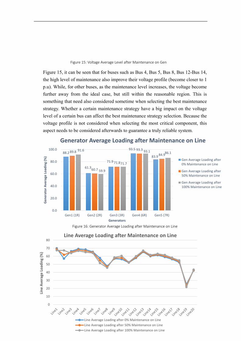
51
Figure 15, it can be seen that for buses such as Bus 4, Bus 5, Bus 8, Bus 12-Bus 14,
the high level of maintenance also improve their voltage profile (become closer to 1
p.u). While, for other buses, as the maintenance level increases, the voltage become
further away from the ideal case, but still within the reasonable region. This is
something that need also considered sometime when selecting the best maintenance
strategy. Whether a certain maintenance strategy have a big impact on the voltage
level of a certain bus can affect the best maintenance strategy selection. Because the
voltage profile is not considered when selecting the most critical component, this
aspect needs to be considered afterwards to guarantee a truly reliable system.
Figure 15: Voltage Average Level after Maintenance on Gen
88.2
61.3
71.9
93.5
83.9
89.8
60.7
71.8
93.3
84.9 91.6
59.9
71.7
93.1 86.1
0.0
20.0
40.0
60.0
80.0
100.0
Gen1 (1R) Gen2 (2R) Gen3 (3R) Gen4 (6R) Gen5 (7R)
Generator Average
Load
ing (%
)
Generators
Generator Average Loading after Maintenance on Line
Gen Average Loading after0% Maintenance on Line
Gen Average Loading after50% Maintenance on Line
Gen Average Loading after100% Maintenance on Line
Figure 16: Generator Average Loading after Maintenance on Line
0
10
20
30
40
50
60
70
80
Line Average
Load
ing (%
)
Line Average Loading after Maintenance on Line
Line Average Loading after 0% Maintenance on Line
Line Average Loading after 50% Maintenance on Line
Line Average Loading after 100% Maintenance on Line
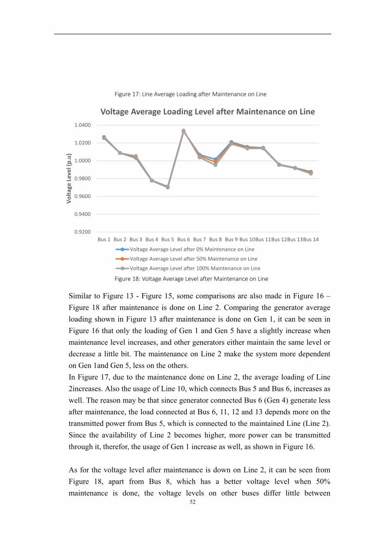
52
Similar to Figure 13 - Figure 15, some comparisons are also made in Figure 16 –
Figure 18 after maintenance is done on Line 2. Comparing the generator average
loading shown in Figure 13 after maintenance is done on Gen 1, it can be seen in
Figure 16 that only the loading of Gen 1 and Gen 5 have a slightly increase when
maintenance level increases, and other generators either maintain the same level or
decrease a little bit. The maintenance on Line 2 make the system more dependent
on Gen 1and Gen 5, less on the others.
In Figure 17, due to the maintenance done on Line 2, the average loading of Line
2increases. Also the usage of Line 10, which connects Bus 5 and Bus 6, increases as
well. The reason may be that since generator connected Bus 6 (Gen 4) generate less
after maintenance, the load connected at Bus 6, 11, 12 and 13 depends more on the
transmitted power from Bus 5, which is connected to the maintained Line (Line 2).
Since the availability of Line 2 becomes higher, more power can be transmitted
through it, therefor, the usage of Gen 1 increase as well, as shown in Figure 16.
As for the voltage level after maintenance is down on Line 2, it can be seen from
Figure 18, apart from Bus 8, which has a better voltage level when 50%
maintenance is done, the voltage levels on other buses differ little between
0.9200
0.9400
0.9600
0.9800
1.0000
1.0200
1.0400
Bus 1 Bus 2 Bus 3 Bus 4 Bus 5 Bus 6 Bus 7 Bus 8 Bus 9 Bus 10Bus 11Bus 12Bus 13Bus 14
Voltage Level (p.u)
Voltage Average Loading Level after Maintenance on Line
Voltage Average Level after 0% Maintenance on Line
Voltage Average Level after 50% Maintenance on Line
Voltage Average Level after 100% Maintenance on Line
Figure 17: Line Average Loading after Maintenance on Line
Figure 18: Voltage Average Level after Maintenance on Line
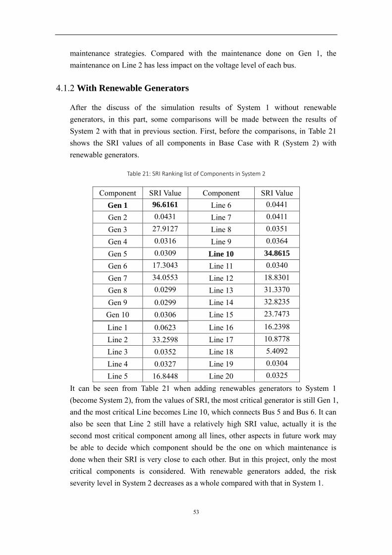
53
maintenance strategies. Compared with the maintenance done on Gen 1, the
maintenance on Line 2 has less impact on the voltage level of each bus.
4.1.2 With Renewable Generators
After the discuss of the simulation results of System 1 without renewable
generators, in this part, some comparisons will be made between the results of
System 2 with that in previous section. First, before the comparisons, in Table 21
shows the SRI values of all components in Base Case with R (System 2) with
renewable generators.
Table 21: SRI Ranking list of Components in System 2
Component SRI Value Component SRI Value
Gen 1 96.6161 Line 6 0.0441
Gen 2 0.0431 Line 7 0.0411
Gen 3 27.9127 Line 8 0.0351
Gen 4 0.0316 Line 9 0.0364
Gen 5 0.0309 Line 10 34.8615
Gen 6 17.3043 Line 11 0.0340
Gen 7 34.0553 Line 12 18.8301
Gen 8 0.0299 Line 13 31.3370
Gen 9 0.0299 Line 14 32.8235
Gen 10 0.0306 Line 15 23.7473
Line 1 0.0623 Line 16 16.2398
Line 2 33.2598 Line 17 10.8778
Line 3 0.0352 Line 18 5.4092
Line 4 0.0327 Line 19 0.0304
Line 5 16.8448 Line 20 0.0325
It can be seen from Table 21 when adding renewables generators to System 1
(become System 2), from the values of SRI, the most critical generator is still Gen 1,
and the most critical Line becomes Line 10, which connects Bus 5 and Bus 6. It can
also be seen that Line 2 still have a relatively high SRI value, actually it is the
second most critical component among all lines, other aspects in future work may
be able to decide which component should be the one on which maintenance is
done when their SRI is very close to each other. But in this project, only the most
critical components is considered. With renewable generators added, the risk
severity level in System 2 decreases as a whole compared with that in System 1.
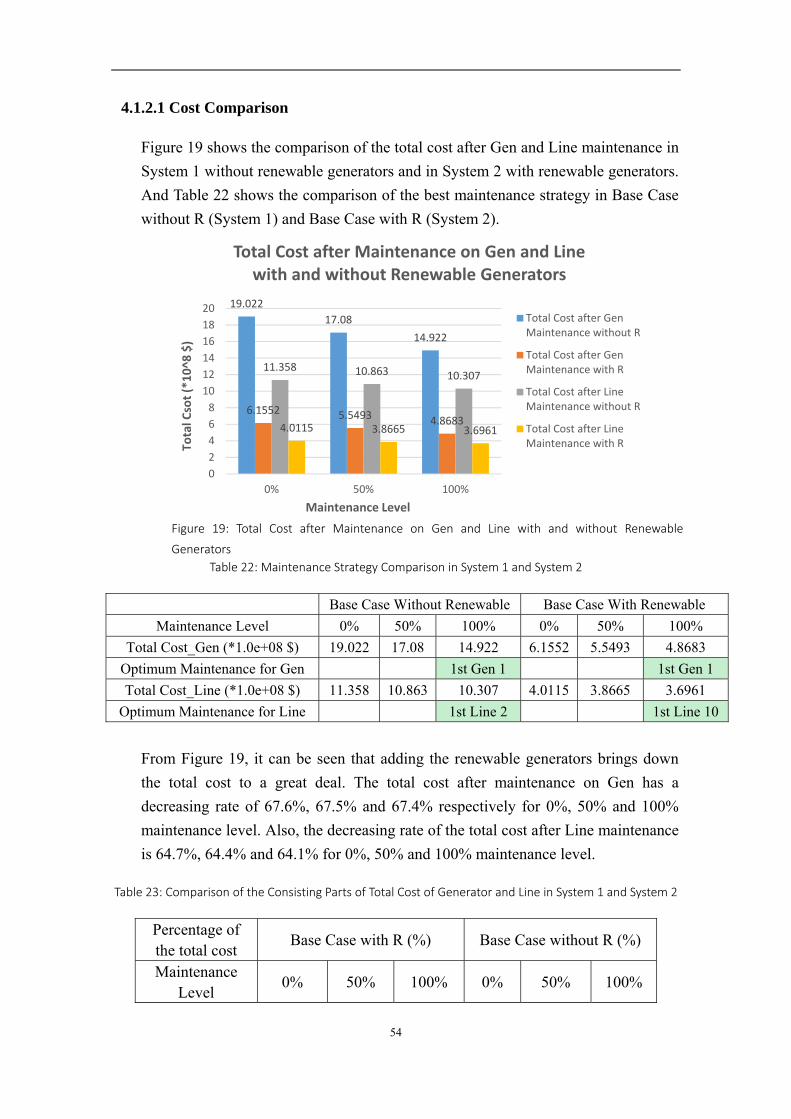
54
4.1.2.1 Cost Comparison
Figure 19 shows the comparison of the total cost after Gen and Line maintenance in
System 1 without renewable generators and in System 2 with renewable generators.
And Table 22 shows the comparison of the best maintenance strategy in Base Case
without R (System 1) and Base Case with R (System 2).
Table 22: Maintenance Strategy Comparison in System 1 and System 2
Base Case Without Renewable Base Case With Renewable
Maintenance Level 0% 50% 100% 0% 50% 100%
Total Cost_Gen (*1.0e+08 $) 19.022 17.08 14.922 6.1552 5.5493 4.8683
Optimum Maintenance for Gen 1st Gen 1 1st Gen 1
Total Cost_Line (*1.0e+08 $) 11.358 10.863 10.307 4.0115 3.8665 3.6961
Optimum Maintenance for Line 1st Line 2 1st Line 10
From Figure 19, it can be seen that adding the renewable generators brings down
the total cost to a great deal. The total cost after maintenance on Gen has a
decreasing rate of 67.6%, 67.5% and 67.4% respectively for 0%, 50% and 100%
maintenance level. Also, the decreasing rate of the total cost after Line maintenance
is 64.7%, 64.4% and 64.1% for 0%, 50% and 100% maintenance level.
Table 23: Comparison of the Consisting Parts of Total Cost of Generator and Line in System 1 and System 2
Percentage of the total cost
Base Case with R (%) Base Case without R (%)
Maintenance Level
0% 50% 100% 0% 50% 100%
19.022
17.08
14.922
6.1552 5.5493 4.8683
11.358 10.863 10.307
4.0115 3.8665 3.6961
0
2
4
6
8
10
12
14
16
18
20
0% 50% 100%
Total Csot (*10^8
$)
Maintenance Level
Total Cost after Maintenance on Gen and Line with and without Renewable Generators
Total Cost after GenMaintenance without R
Total Cost after GenMaintenance with R
Total Cost after LineMaintenance without R
Total Cost after LineMaintenance with R
Figure 19: Total Cost after Maintenance on Gen and Line with and without Renewable
Generators
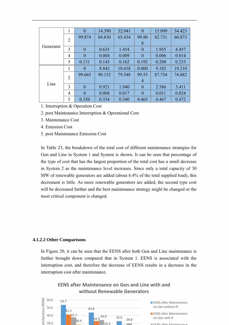
55
Generator
1 0 14.390 32.941 0 15.099 34.423
2 99.874 84.830 65.434 99.80
8 82.731 60.873
3 0 0.635 1.454 0 1.955 4.457 4 0 0.004 0.009 0 0.006 0.014 5 0.131 0.143 0.162 0.192 0.208 0.233
Line
1 0 8.842 18.638 0.000 9.182 19.210
2 99.665 90.132 79.548 99.53
4 87.754 74.882
3 0 0.921 1.940 0 2.586 5.411 4 0 0.008 0.017 0 0.011 0.024 5 0.330 0.334 0.340 0.465 0.467 0.472
1. Interruption & Operation Cost
2. post Maintenance Interruption & Operational Cost
3. Maintenance Cost
4. Emission Cost
5. post Maintenance Emission Cost
In Table 23, the breakdown of the total cost of different maintenance strategies for
Gen and Line in System 1 and System is shown. It can be seen that percentage of
the type of cost that has the largest proportion of the total cost has a small decrease
in System 2 as the maintenance level increases. Since only a total capacity of 30
MW of renewable generators are added (about 6.4% of the total supplied load), this
decrement is little. As more renewable generators are added, the second type cost
will be decreased further and the best maintenance strategy might be changed or the
most critical component is changed.
4.1.2.2 Other Comparisons
In Figure 20, it can be seen that the EENS after both Gen and Line maintenance is
further brought down compared that in System 1. EENS is associated with the
interruption cost, and therefore the decrease of EENS results in a decrease in the
interruption cost after maintenance.
53.7
43.8
32.6
41.3
32.9
23 3
37.7 34.0 29.8 28.4
25.5 30.0
40.0
50.0
60.0
aintenance (MW)
EENS after Maintenance on Gen and Line with and without Renewable Generators
EENS after Maintenanceon Gen without R
EENS after Maintenanceon Gen with R
EENS after Maintenance
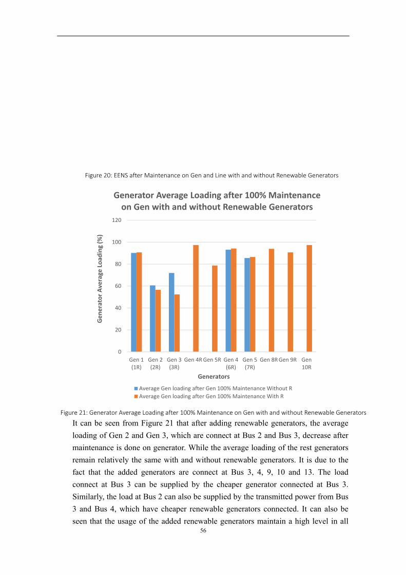
56
It can be seen from Figure 21 that after adding renewable generators, the average
loading of Gen 2 and Gen 3, which are connect at Bus 2 and Bus 3, decrease after
maintenance is done on generator. While the average loading of the rest generators
remain relatively the same with and without renewable generators. It is due to the
fact that the added generators are connect at Bus 3, 4, 9, 10 and 13. The load
connect at Bus 3 can be supplied by the cheaper generator connected at Bus 3.
Similarly, the load at Bus 2 can also be supplied by the transmitted power from Bus
3 and Bus 4, which have cheaper renewable generators connected. It can also be
seen that the usage of the added renewable generators maintain a high level in all
Figure 20: EENS after Maintenance on Gen and Line with and without Renewable Generators
Figure 21: Generator Average Loading after 100% Maintenance on Gen with and without Renewable Generators
0
20
40
60
80
100
120
Gen 1(1R)
Gen 2(2R)
Gen 3(3R)
Gen 4RGen 5R Gen 4(6R)
Gen 5(7R)
Gen 8RGen 9R Gen10R
Generator Average
Load
ing (%
)
Generators
Generator Average Loading after 100% Maintenance on Gen with and without Renewable Generators
Average Gen loading after Gen 100% Maintenance Without R
Average Gen loading after Gen 100% Maintenance With R
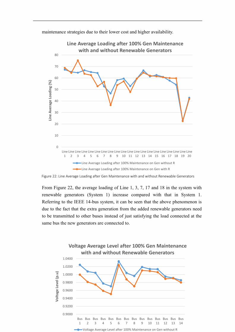
57
maintenance strategies due to their lower cost and higher availability.
From Figure 22, the average loading of Line 1, 3, 7, 17 and 18 in the system with
renewable generators (System 1) increase compared with that in System 1.
Referring to the IEEE 14-bus system, it can be seen that the above phenomenon is
due to the fact that the extra generation from the added renewable generators need
to be transmitted to other buses instead of just satisfying the load connected at the
same bus the new generators are connected to.
Figure 22: Line Average Loading after Gen Maintenance with and without Renewable Generators
0.9000
0.9200
0.9400
0.9600
0.9800
1.0000
1.0200
1.0400
Bus1
Bus2
Bus3
Bus4
Bus5
Bus6
Bus7
Bus8
Bus9
Bus10
Bus11
Bus12
Bus13
Bus14
Voltage Level (p.u)
Voltage Average Level after 100% Gen Maintenance with and without Renewable Generators
Voltage Average Level after 100% Maintenance on Gen without R
0
10
20
30
40
50
60
70
80
Line1
Line2
Line3
Line4
Line5
Line6
Line7
Line8
Line9
Line10
Line11
Line12
Line13
Line14
Line15
Line16
Line17
Line18
Line19
Line20
Line Average
Load
ing (%
)
Line Average Loading after 100% Gen Maintenance with and without Renewable Generators
Line Average Loading after 100% Maintenance on Gen without R
Line Average Loading after 100% Maintenance on Gen with R
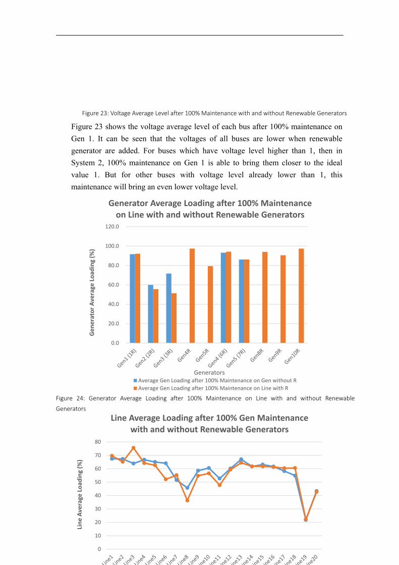
58
Figure 23 shows the voltage average level of each bus after 100% maintenance on
Gen 1. It can be seen that the voltages of all buses are lower when renewable
generator are added. For buses which have voltage level higher than 1, then in
System 2, 100% maintenance on Gen 1 is able to bring them closer to the ideal
value 1. But for other buses with voltage level already lower than 1, this
maintenance will bring an even lower voltage level.
Figure 23: Voltage Average Level after 100% Maintenance with and without Renewable Generators
0.0
20.0
40.0
60.0
80.0
100.0
120.0
Generator Average
Load
ing (%
)
Generators
Generator Average Loading after 100% Maintenance on Line with and without Renewable Generators
Average Gen Loading after 100% Maintenance on Gen without R
Average Gen Loading after 100% Maintenance on Line with R
Figure 24: Generator Average Loading after 100% Maintenance on Line with and without Renewable
Generators
0
10
20
30
40
50
60
70
80
Line Average
Load
ing (%
)
Line Average Loading after 100% Gen Maintenance with and without Renewable Generators
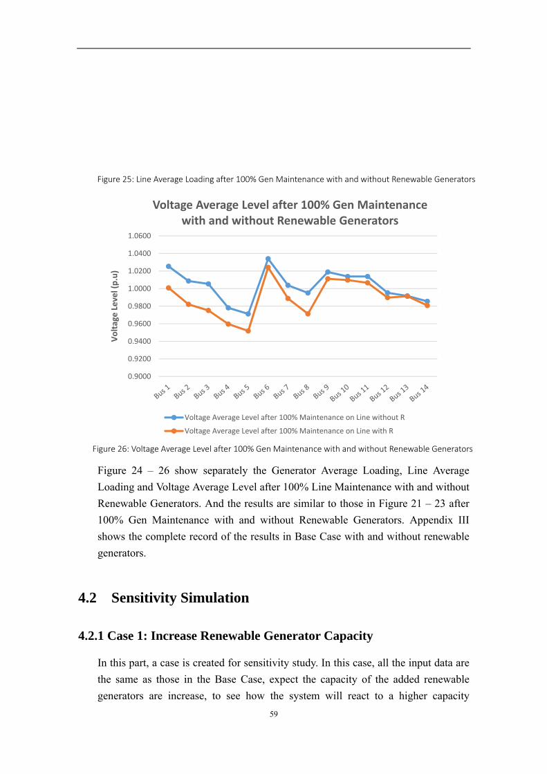
59
Figure 24 – 26 show separately the Generator Average Loading, Line Average
Loading and Voltage Average Level after 100% Line Maintenance with and without
Renewable Generators. And the results are similar to those in Figure 21 – 23 after
100% Gen Maintenance with and without Renewable Generators. Appendix III
shows the complete record of the results in Base Case with and without renewable
generators.
4.2 Sensitivity Simulation
4.2.1 Case 1: Increase Renewable Generator Capacity
In this part, a case is created for sensitivity study. In this case, all the input data are
the same as those in the Base Case, expect the capacity of the added renewable
generators are increase, to see how the system will react to a higher capacity
Figure 25: Line Average Loading after 100% Gen Maintenance with and without Renewable Generators
0.9000
0.9200
0.9400
0.9600
0.9800
1.0000
1.0200
1.0400
1.0600
Voltage Level (p.u)
Voltage Average Level after 100% Gen Maintenance with and without Renewable Generators
Voltage Average Level after 100% Maintenance on Line without R
Voltage Average Level after 100% Maintenance on Line with R
Figure 26: Voltage Average Level after 100% Gen Maintenance with and without Renewable Generators
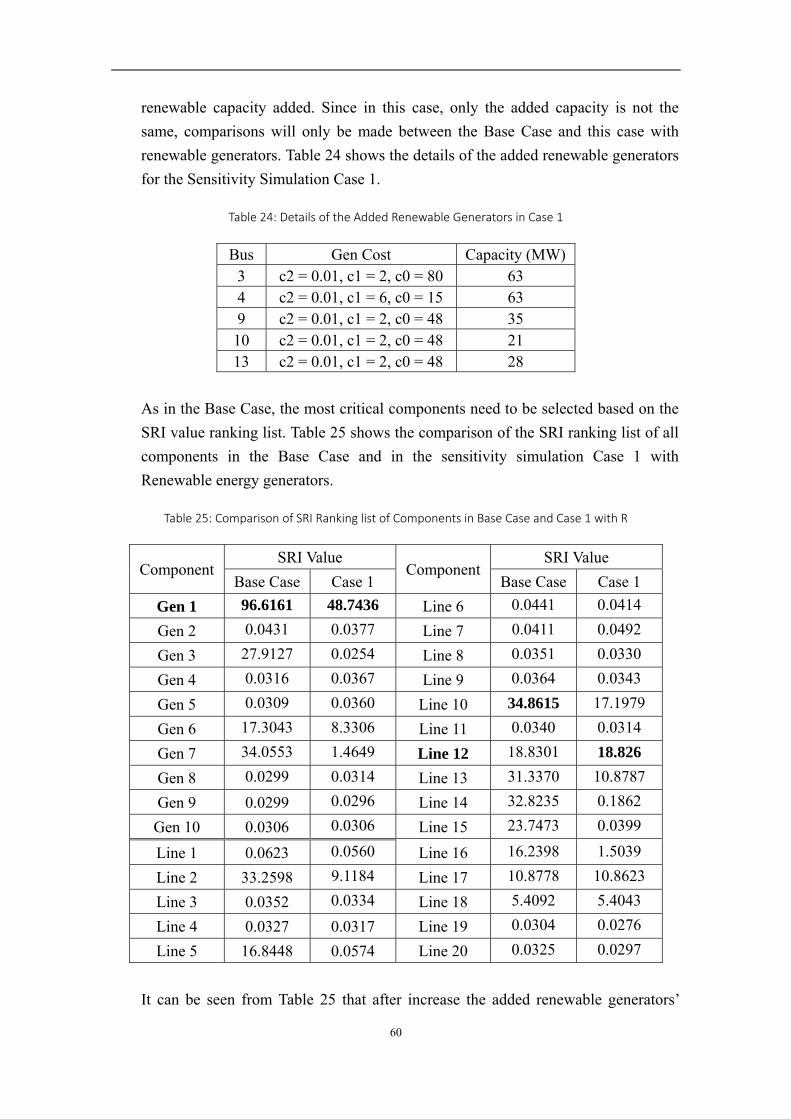
60
renewable capacity added. Since in this case, only the added capacity is not the
same, comparisons will only be made between the Base Case and this case with
renewable generators. Table 24 shows the details of the added renewable generators
for the Sensitivity Simulation Case 1.
Table 24: Details of the Added Renewable Generators in Case 1
Bus Gen Cost Capacity (MW) 3 c2 = 0.01, c1 = 2, c0 = 80 63 4 c2 = 0.01, c1 = 6, c0 = 15 63 9 c2 = 0.01, c1 = 2, c0 = 48 35 10 c2 = 0.01, c1 = 2, c0 = 48 21 13 c2 = 0.01, c1 = 2, c0 = 48 28
As in the Base Case, the most critical components need to be selected based on the
SRI value ranking list. Table 25 shows the comparison of the SRI ranking list of all
components in the Base Case and in the sensitivity simulation Case 1 with
Renewable energy generators.
Table 25: Comparison of SRI Ranking list of Components in Base Case and Case 1 with R
Component SRI Value
Component SRI Value
Base Case Case 1 Base Case Case 1
Gen 1 96.6161 48.7436 Line 6 0.0441 0.0414
Gen 2 0.0431 0.0377 Line 7 0.0411 0.0492
Gen 3 27.9127 0.0254 Line 8 0.0351 0.0330
Gen 4 0.0316 0.0367 Line 9 0.0364 0.0343
Gen 5 0.0309 0.0360 Line 10 34.8615 17.1979
Gen 6 17.3043 8.3306 Line 11 0.0340 0.0314
Gen 7 34.0553 1.4649 Line 12 18.8301 18.826
Gen 8 0.0299 0.0314 Line 13 31.3370 10.8787
Gen 9 0.0299 0.0296 Line 14 32.8235 0.1862
Gen 10 0.0306 0.0306 Line 15 23.7473 0.0399
Line 1 0.0623 0.0560 Line 16 16.2398 1.5039
Line 2 33.2598 9.1184 Line 17 10.8778 10.8623
Line 3 0.0352 0.0334 Line 18 5.4092 5.4043
Line 4 0.0327 0.0317 Line 19 0.0304 0.0276
Line 5 16.8448 0.0574 Line 20 0.0325 0.0297
It can be seen from Table 25 that after increase the added renewable generators’
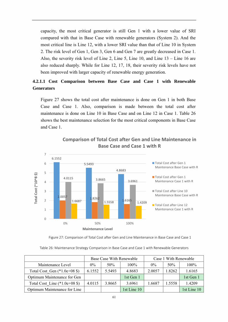
61
capacity, the most critical generator is still Gen 1 with a lower value of SRI
compared with that in Base Case with renewable generators (System 2). And the
most critical line is Line 12, with a lower SRI value than that of Line 10 in System
2. The risk level of Gen 1, Gen 3, Gen 6 and Gen 7 are greatly decreased in Case 1.
Also, the severity risk level of Line 2, Line 5, Line 10, and Line 13 – Line 16 are
also reduced sharply. While for Line 12, 17, 18, their severity risk levels have not
been improved with larger capacity of renewable energy generation.
4.2.1.1 Cost Comparison between Base Case and Case 1 with Renewable
Generators
Figure 27 shows the total cost after maintenance is done on Gen 1 in both Base
Case and Case 1. Also, comparison is made between the total cost after
maintenance is done on Line 10 in Base Case and on Line 12 in Case 1. Table 26
shows the best maintenance selection for the most critical components in Base Case
and Case 1.
Table 26: Maintenance Strategy Comparison in Base Case and Case 1 with Renewable Generators
Base Case With Renewable Case 1 With Renewable
Maintenance Level 0% 50% 100% 0% 50% 100%
Total Cost_Gen (*1.0e+08 $) 6.1552 5.5493 4.8683 2.0057 1.8262 1.6165
Optimum Maintenance for Gen 1st Gen 1 1st Gen 1
Total Cost_Line (*1.0e+08 $) 4.0115 3.8665 3.6961 1.6687 1.5558 1.4209
Optimum Maintenance for Line 1st Line 10 1st Line 10
6.1552
5.5493
4.8683
2.0057 1.82621.6165
4.0115 3.8665 3.6961
1.6687 1.5558 1.4209
0
1
2
3
4
5
6
7
0% 50% 100%
Total Cost (*10^8
$)
Maintenance Level
Comparison of Total Cost after Gen and Line Maintenance in Base Case and Case 1 with R
Total Cost after Gen 1Maintenance Base Case with R
Total Cost after Gen 1Maintenance Case 1 with R
Total Cost after Line 10Maintenance Base Case with R
Total Cost after Line 12Maintenance Case 1 with R
Figure 27: Comparison of Total Cost after Gen and Line Maintenance in Base Case and Case 1
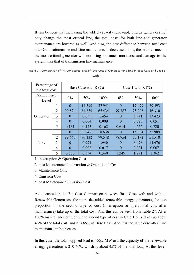
62
It can be seen that increasing the added capacity renewable energy generators not
only change the most critical line, the total costs for both line and generator
maintenance are lowered as well. And also, the cost difference between total cost
after Gen maintenance and Line maintenance is decreased, thus, the maintenance on
the most critical generator will not bring too much more cost and damage to the
system than that of transmission line maintenance.
Table 27: Comparison of the Consisting Parts of Total Cost of Generator and Line in Base Case and Case 1
with R
Percentage of the total cost
Base Case with R (%) Case 1 with R (%)
Maintenance Level
0% 50% 100% 0% 50% 100%
Generator
1 0 14.390 32.941 0 17.479 39.493 2 99.874 84.830 65.434 99.387 75.906 46.310 3 0 0.635 1.454 0 5.941 13.423 4 0 0.004 0.009 0 0.023 0.051 5 0.131 0.143 0.162 0.614 0.656 0.720
Line
1 0 8.842 18.638 0 15.064 32.989 2 99.665 90.132 79.548 98.754 77.182 51.510 3 0 0.921 1.940 0 6.428 14.076 4 0 0.008 0.017 0 0.031 0.067 5 0.330 0.334 0.340 1.249 1.291 1.362
1. Interruption & Operation Cost
2. post Maintenance Interruption & Operational Cost
3. Maintenance Cost
4. Emission Cost
5. post Maintenance Emission Cost
As discussed in 4.1.2.1 Cost Comparison between Base Case with and without
Renewable Generators, the more the added renewable energy generators, the less
proportion of the second type of cost (interruption & operational cost after
maintenance) take up of the total cost. And this can be seen from Table 27. After
100% maintenance on Gen 1, the second type of cost in Case 1 only takes up about
46% of the total cost, and it is 65% in Base Case. And it is the same case after Line
maintenance in both cases.
In this case, the total supplied load is 466.2 MW and the capacity of the renewable
energy generation is 210 MW, which is about 45% of the total load. At this level,
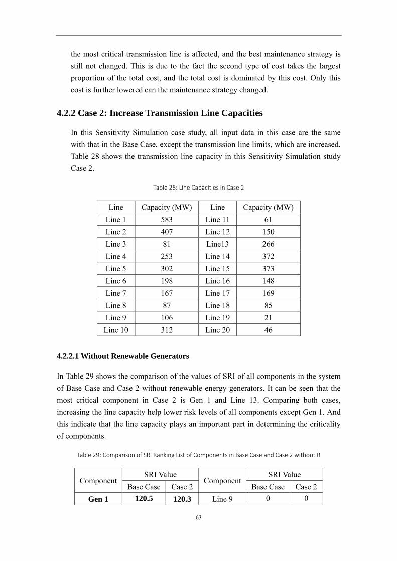
63
the most critical transmission line is affected, and the best maintenance strategy is
still not changed. This is due to the fact the second type of cost takes the largest
proportion of the total cost, and the total cost is dominated by this cost. Only this
cost is further lowered can the maintenance strategy changed.
4.2.2 Case 2: Increase Transmission Line Capacities
In this Sensitivity Simulation case study, all input data in this case are the same
with that in the Base Case, except the transmission line limits, which are increased.
Table 28 shows the transmission line capacity in this Sensitivity Simulation study
Case 2.
Table 28: Line Capacities in Case 2
Line Capacity (MW) Line Capacity (MW)
Line 1 583 Line 11 61
Line 2 407 Line 12 150
Line 3 81 Line13 266
Line 4 253 Line 14 372
Line 5 302 Line 15 373
Line 6 198 Line 16 148
Line 7 167 Line 17 169
Line 8 87 Line 18 85
Line 9 106 Line 19 21
Line 10 312 Line 20 46
4.2.2.1 Without Renewable Generators
In Table 29 shows the comparison of the values of SRI of all components in the system
of Base Case and Case 2 without renewable energy generators. It can be seen that the
most critical component in Case 2 is Gen 1 and Line 13. Comparing both cases,
increasing the line capacity help lower risk levels of all components except Gen 1. And
this indicate that the line capacity plays an important part in determining the criticality
of components.
Table 29: Comparison of SRI Ranking List of Components in Base Case and Case 2 without R
Component SRI Value
Component SRI Value
Base Case Case 2 Base Case Case 2
Gen 1 120.5 120.3 Line 9 0 0
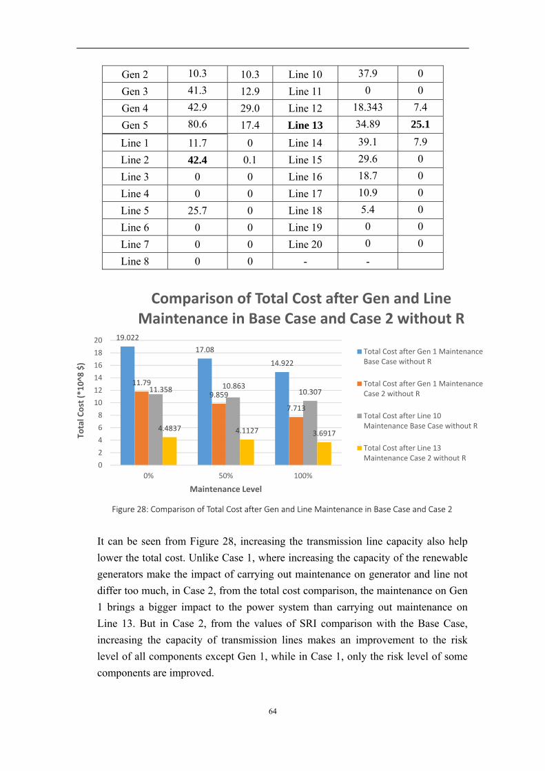
64
Gen 2 10.3 10.3 Line 10 37.9 0
Gen 3 41.3 12.9 Line 11 0 0
Gen 4 42.9 29.0 Line 12 18.343 7.4
Gen 5 80.6 17.4 Line 13 34.89 25.1
Line 1 11.7 0 Line 14 39.1 7.9
Line 2 42.4 0.1 Line 15 29.6 0
Line 3 0 0 Line 16 18.7 0
Line 4 0 0 Line 17 10.9 0
Line 5 25.7 0 Line 18 5.4 0
Line 6 0 0 Line 19 0 0
Line 7 0 0 Line 20 0 0
Line 8 0 0 - -
It can be seen from Figure 28, increasing the transmission line capacity also help
lower the total cost. Unlike Case 1, where increasing the capacity of the renewable
generators make the impact of carrying out maintenance on generator and line not
differ too much, in Case 2, from the total cost comparison, the maintenance on Gen
1 brings a bigger impact to the power system than carrying out maintenance on
Line 13. But in Case 2, from the values of SRI comparison with the Base Case,
increasing the capacity of transmission lines makes an improvement to the risk
level of all components except Gen 1, while in Case 1, only the risk level of some
components are improved.
19.022
17.08
14.922
11.79
9.859
7.713
11.358 10.86310.307
4.4837 4.1127 3.6917
0
2
4
6
8
10
12
14
16
18
20
0% 50% 100%
Total Cost (*10^8
$)
Maintenance Level
Comparison of Total Cost after Gen and Line Maintenance in Base Case and Case 2 without R
Total Cost after Gen 1 MaintenanceBase Case without R
Total Cost after Gen 1 MaintenanceCase 2 without R
Total Cost after Line 10Maintenance Base Case without R
Total Cost after Line 13Maintenance Case 2 without R
Figure 28: Comparison of Total Cost after Gen and Line Maintenance in Base Case and Case 2
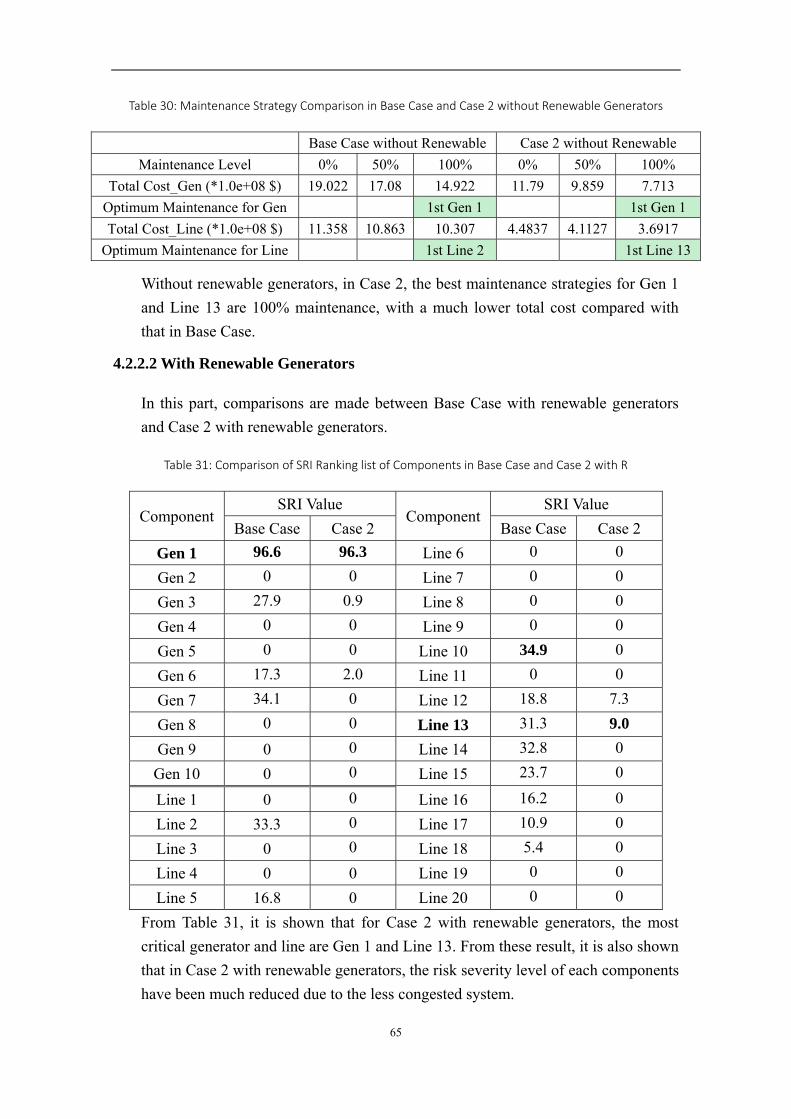
65
Table 30: Maintenance Strategy Comparison in Base Case and Case 2 without Renewable Generators
Base Case without Renewable Case 2 without Renewable
Maintenance Level 0% 50% 100% 0% 50% 100%
Total Cost_Gen (*1.0e+08 $) 19.022 17.08 14.922 11.79 9.859 7.713
Optimum Maintenance for Gen 1st Gen 1 1st Gen 1
Total Cost_Line (*1.0e+08 $) 11.358 10.863 10.307 4.4837 4.1127 3.6917
Optimum Maintenance for Line 1st Line 2 1st Line 13
Without renewable generators, in Case 2, the best maintenance strategies for Gen 1
and Line 13 are 100% maintenance, with a much lower total cost compared with
that in Base Case.
4.2.2.2 With Renewable Generators
In this part, comparisons are made between Base Case with renewable generators
and Case 2 with renewable generators.
Table 31: Comparison of SRI Ranking list of Components in Base Case and Case 2 with R
Component SRI Value
Component SRI Value
Base Case Case 2 Base Case Case 2
Gen 1 96.6 96.3 Line 6 0 0
Gen 2 0 0 Line 7 0 0
Gen 3 27.9 0.9 Line 8 0 0
Gen 4 0 0 Line 9 0 0
Gen 5 0 0 Line 10 34.9 0
Gen 6 17.3 2.0 Line 11 0 0
Gen 7 34.1 0 Line 12 18.8 7.3
Gen 8 0 0 Line 13 31.3 9.0
Gen 9 0 0 Line 14 32.8 0
Gen 10 0 0 Line 15 23.7 0
Line 1 0 0 Line 16 16.2 0
Line 2 33.3 0 Line 17 10.9 0
Line 3 0 0 Line 18 5.4 0
Line 4 0 0 Line 19 0 0
Line 5 16.8 0 Line 20 0 0
From Table 31, it is shown that for Case 2 with renewable generators, the most
critical generator and line are Gen 1 and Line 13. From these result, it is also shown
that in Case 2 with renewable generators, the risk severity level of each components
have been much reduced due to the less congested system.
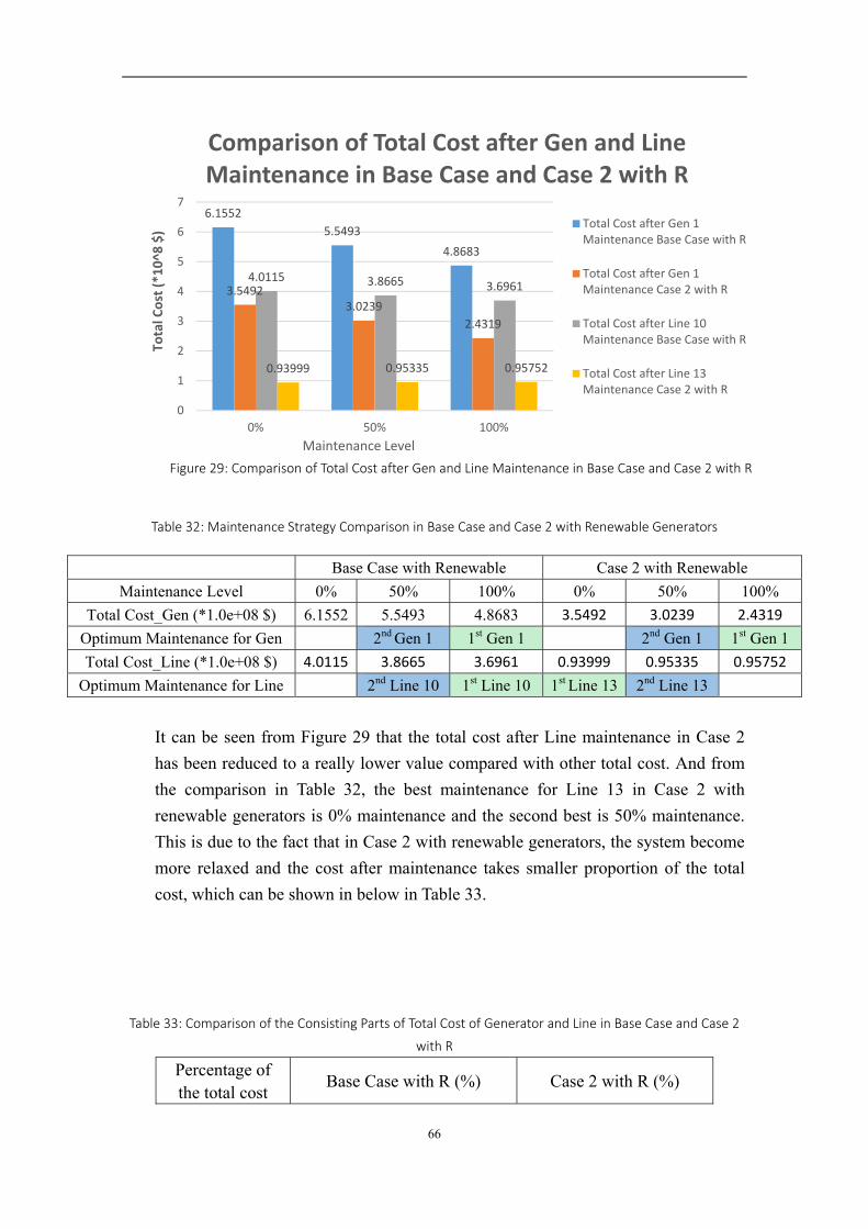
66
Table 32: Maintenance Strategy Comparison in Base Case and Case 2 with Renewable Generators
Base Case with Renewable Case 2 with Renewable
Maintenance Level 0% 50% 100% 0% 50% 100%
Total Cost_Gen (*1.0e+08 $) 6.1552 5.5493 4.8683 3.5492 3.0239 2.4319
Optimum Maintenance for Gen 2nd Gen 1 1st Gen 1 2nd Gen 1 1st Gen 1
Total Cost_Line (*1.0e+08 $) 4.0115 3.8665 3.6961 0.93999 0.95335 0.95752
Optimum Maintenance for Line 2nd Line 10 1st Line 10 1st Line 13 2nd Line 13
It can be seen from Figure 29 that the total cost after Line maintenance in Case 2
has been reduced to a really lower value compared with other total cost. And from
the comparison in Table 32, the best maintenance for Line 13 in Case 2 with
renewable generators is 0% maintenance and the second best is 50% maintenance.
This is due to the fact that in Case 2 with renewable generators, the system become
more relaxed and the cost after maintenance takes smaller proportion of the total
cost, which can be shown in below in Table 33.
Table 33: Comparison of the Consisting Parts of Total Cost of Generator and Line in Base Case and Case 2
with R
Percentage of the total cost
Base Case with R (%) Case 2 with R (%)
6.1552
5.5493
4.8683
3.54923.0239
2.4319
4.0115 3.8665 3.6961
0.93999 0.95335 0.95752
0
1
2
3
4
5
6
7
0% 50% 100%
Total Cost (*10^8
$)
Maintenance Level
Comparison of Total Cost after Gen and Line Maintenance in Base Case and Case 2 with R
Total Cost after Gen 1Maintenance Base Case with R
Total Cost after Gen 1Maintenance Case 2 with R
Total Cost after Line 10Maintenance Base Case with R
Total Cost after Line 13Maintenance Case 2 with R
Figure 29: Comparison of Total Cost after Gen and Line Maintenance in Base Case and Case 2 with R
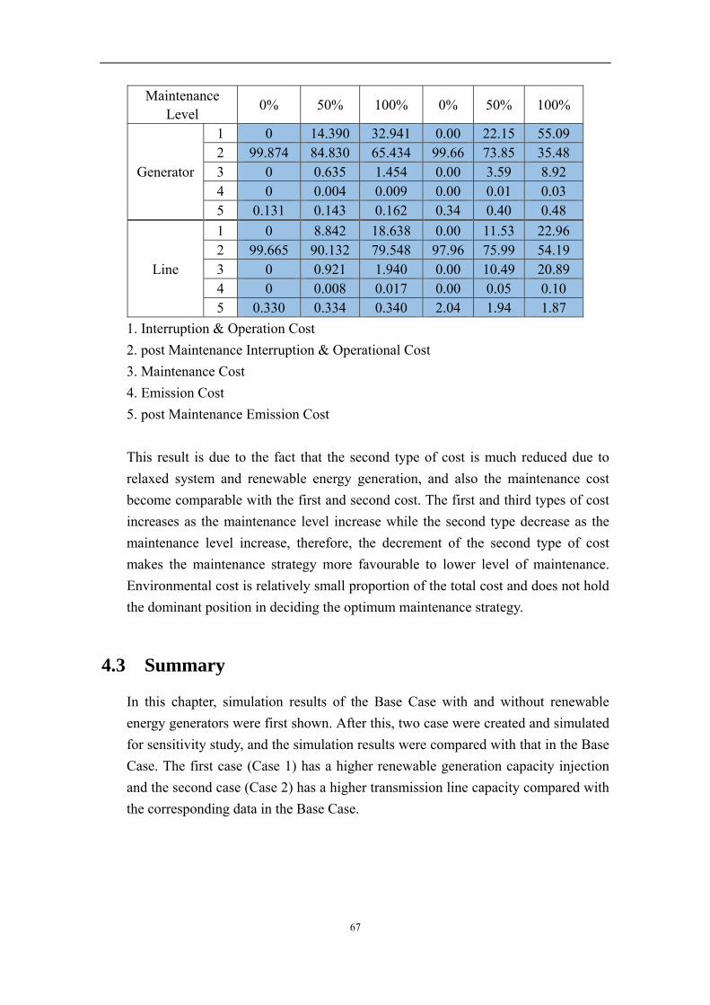
67
Maintenance Level
0% 50% 100% 0% 50% 100%
Generator
1 0 14.390 32.941 0.00 22.15 55.09 2 99.874 84.830 65.434 99.66 73.85 35.48 3 0 0.635 1.454 0.00 3.59 8.92 4 0 0.004 0.009 0.00 0.01 0.03 5 0.131 0.143 0.162 0.34 0.40 0.48
Line
1 0 8.842 18.638 0.00 11.53 22.96 2 99.665 90.132 79.548 97.96 75.99 54.19 3 0 0.921 1.940 0.00 10.49 20.89 4 0 0.008 0.017 0.00 0.05 0.10 5 0.330 0.334 0.340 2.04 1.94 1.87
1. Interruption & Operation Cost
2. post Maintenance Interruption & Operational Cost
3. Maintenance Cost
4. Emission Cost
5. post Maintenance Emission Cost
This result is due to the fact that the second type of cost is much reduced due to
relaxed system and renewable energy generation, and also the maintenance cost
become comparable with the first and second cost. The first and third types of cost
increases as the maintenance level increase while the second type decrease as the
maintenance level increase, therefore, the decrement of the second type of cost
makes the maintenance strategy more favourable to lower level of maintenance.
Environmental cost is relatively small proportion of the total cost and does not hold
the dominant position in deciding the optimum maintenance strategy.
4.3 Summary
In this chapter, simulation results of the Base Case with and without renewable
energy generators were first shown. After this, two case were created and simulated
for sensitivity study, and the simulation results were compared with that in the Base
Case. The first case (Case 1) has a higher renewable generation capacity injection
and the second case (Case 2) has a higher transmission line capacity compared with
the corresponding data in the Base Case.
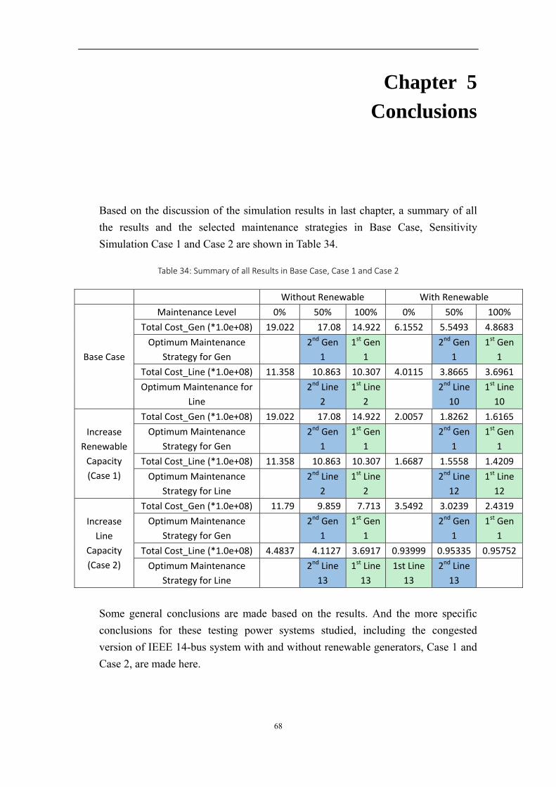
68
Chapter 5
Conclusions
Based on the discussion of the simulation results in last chapter, a summary of all
the results and the selected maintenance strategies in Base Case, Sensitivity
Simulation Case 1 and Case 2 are shown in Table 34.
Table 34: Summary of all Results in Base Case, Case 1 and Case 2
Without Renewable With Renewable
Base Case
Maintenance Level 0% 50% 100% 0% 50% 100%
Total Cost_Gen (*1.0e+08) 19.022 17.08 14.922 6.1552 5.5493 4.8683
Optimum Maintenance
Strategy for Gen
2nd Gen
1
1st Gen
1
2nd Gen
1
1st Gen
1
Total Cost_Line (*1.0e+08) 11.358 10.863 10.307 4.0115 3.8665 3.6961
Optimum Maintenance for
Line
2nd Line
2
1st Line
2
2nd Line
10
1st Line
10
Increase
Renewable
Capacity
(Case 1)
Total Cost_Gen (*1.0e+08) 19.022 17.08 14.922 2.0057 1.8262 1.6165
Optimum Maintenance
Strategy for Gen
2nd Gen
1
1st Gen
1
2nd Gen
1
1st Gen
1
Total Cost_Line (*1.0e+08) 11.358 10.863 10.307 1.6687 1.5558 1.4209
Optimum Maintenance
Strategy for Line
2nd Line
2
1st Line
2
2nd Line
12
1st Line
12
Increase
Line
Capacity
(Case 2)
Total Cost_Gen (*1.0e+08) 11.79 9.859 7.713 3.5492 3.0239 2.4319
Optimum Maintenance
Strategy for Gen
2nd Gen
1
1st Gen
1
2nd Gen
1
1st Gen
1
Total Cost_Line (*1.0e+08) 4.4837 4.1127 3.6917 0.93999 0.95335 0.95752
Optimum Maintenance
Strategy for Line
2nd Line
13
1st Line
13
1st Line
13
2nd Line
13
Some general conclusions are made based on the results. And the more specific
conclusions for these testing power systems studied, including the congested
version of IEEE 14-bus system with and without renewable generators, Case 1 and
Case 2, are made here.
69
General conclusions:
1. From the aspects of total cost and EENS, the maintenance for generators often
brings a bigger impact to the power system than the maintenance for
transmission lines in all levels of maintenance.
2. Interruption & Operational cost during and after maintenance take the largest
proportion of the total cost and most of the time dominant the maintenance
strategy selection.
3. With renewable energy generators added, the total cost can be much reduced
and some of the generators and lines can be less loaded, which meanwhile
reduced the risk level of each component.
4. The maintenance of a generator can make the system become more dependent
on some of the transmission lines, which should be paid attention to in order to
avoid potential fault.
5. Similarly, the maintenance of a transmission line can make the system more
dependent on some generators.
6. Between different levels of maintenance, higher degree of maintenance for
generators makes a faster decrement of the total cost and a better improvement
of EENS than the same level of maintenance of transmission lines.
7. Maintenance on a certain component brings different impact on the voltage
level of different buses and this should be considered selecting maintenance
strategy in order to keep all voltages at a reasonable level.
Specific Conclusions:
1. Adding renewable energy generators can change the critical components, in this
study, most probably transmission lines, rather than generators.
2. In the sensitivity simulation case 1, the increment of the added renewable
energy capacity reduces the risk level of Gen 1, Gen 3, Gen 6 and Gen 7, Line 2,
Line 5, Line 10, and Line 13 – Line 16. And the most critical line is changed to
Line 12 with and without renewable generator.
3. With different amount of the capacity of the added renewable energy generators,
the criticality of each components will change, thus the most critical component
can also be changed.
4. In the sensitivity simulation case 2, the increment of the line capacity reduce the
risk level of all components except Gen 1. And the most critical line is Line 13.
5. In a not so congested system, like case 2, the adding of renewable energy
generators can change the selection of the maintenance strategy.
70
Chapter 6
Recommendations and Future Work
There are certainly some constraints and assumptions in this project, the following
are some of the suggested work for the future to make this topic more
comprehensive and complete.
1. Only three levels of maintenance are considered in this project as maintenance
strategies. In the future, more detailed maintenance types can be added.
2. All the maintenance considered here are so called off-line maintenance. Live &
Opportunistic maintenance may also be considered.
3. When calculating the number of consumer interrupted, customers can be
distinguished by types: residential, commercial and industrial. Also, some
important customer such as hospital can be one type of customer to be paid
special attention to.
4. More real-life data can be used in the simulation to get a result related to
industry events.
5. More detailed and quantified study on the impact of transmission line capacity
on the criticality of each component and the maintenance strategy study.
6. Try this method on a larger power system, such as IEEE case 30.

71
72
References [1] Wenyuan LI (2005). Risk Assessment of Power Systems Models, Methods, and Applications. United States of America: A JOHN WILEY & SONS, INC., PUBLICATION. CHAPTER 10 p215-p219. [2] Application, F. & Studies, C., May, 1999. Reliability Centred Maintenance for (RCM) Distribution Systems and Equipment Four Application Case Studies. [3] P. Hilber, “Maintenance Optimization for Power Distribution System”, Doctoral Thesis, School of Electrical Engineering, KTH, Stockholm, Sweden, 2008, ISBN 978-91-628-7464-3. [4] Lina Bertling, Reliability Centred Maintenance for Electric Power System, Doctoral Dissertation, School of Electrical Engineering, KTH, Stockholm, Sweden, 2008, ISBN 91-7283-345-9. [5] B. Yssaad, M. Khiat, and a. Chaker, “Reliability centered maintenance optimization for power distribution systems,” Int. J. Electr. Power Energy Syst., vol. 55, pp. 108–115, 2014. [6] Roy Billinton, Ronald N.Allan (1984). Reliability Evaluation of Power System. 2nd ed. Great Britain: Pitman Book Limited. p6-p16. [7] North American Electric Reliability Corporate, Reliability Assessment Guidebook, version 3.1, August 2012. [8] Zhang, P., Meng, K. & Dong, Z., 2010. Probabilistic vs deterministic power system stability and reliability assessment. Emerging Techniques in Power System Analysis, pp.117–145. [9] R. Allan and R. Billinton, “Probabilistic assessment of power systems,” Proc. IEEE, vol. 88, no. 2, 2000. [10] Wang Peng, NTU EE6510 Power System Operation and Planning Lecture Notes, Example 2-6. [11] José Fernando Prada. (June 1999). The Value of Reliability in Power Systems-Pricing Operating Reserves. Energy Laboratory, Massachusetts Institute of Technology. MIT EL 99-005 WP (1), p12-p32. [12] IEEE/PES Working Group on System Design, “A survey of distribution reliability measurement practices in the U.S.,” IEEE Trans. Power Delivery, vol. 14, no. 1, pp. 250–257, Jan. 1999. [13] IEEE Power & Energy Society. (31 May 2012). IEEE Guide for Electric Power Distribution Reliability Indices. IEEE Standards Association. Std 1366-2003 (3. Definitions of reliability indices), p4-p11. [14] J.Moubray. Reliability-Centred Maintenance. Butterworth-Heinemann, Oxford, 1991. Reprint 1995. [15] F.Stanley Nowlan, Howard F.Heap. (1978). Chapter 1 RCM: Maintenance Disipline. In: Reliability-Centered Maintenance. U.S. Department of Commerce, Springfield, Virginia. p3. [16] N. Cotaina, F. Matos, J. Chabrol, D. Djeapragache, P. Prete, J. Carretero, F. García, M. Pérez, J.M. Peña, J.M. Pérez. (2000). Facultad de Informática de Madrid, UPM, in
73
Campus de Montengancedo, Madrid, Spain. Study of Existing RCM Approaches used in Different Industries. Technical Report, Project Number: 2000 RD 10810. FIM/110.1/DATSI/00 29-06-2000-06-29 (3), p16-p49. [17] John W. Goodfellow. (2000). Applying Reliability Centered Maintenance (RCM) to Overhead Electric Utility Distribution Systems. IEEE. 0-7803-6420-1, p566-p569. [18] ANTHONY UWAKHONYE ADOGHE. (2000). Reliability Centered Maintenance (RCM) for Asset Management in Electric Power Distribution System. Postgraduate thesis submitted in the department of electrical and information engineering, University OTA, Ogun State, Nigeria. [19] Dr. Marhs Zdrallek. (2004). Reliability Centred Maintenance Strategy for High-Voltage-Networks. 8th International Conference on Probabilistic Methods Applied to Power Systems, Iowa State University, Ames, Iowa, September 12-16, 2004. [20] Ebrahim Shayesteh. Project Proposal: Maintenance Optimization of Electric Power System (2015). [21] SKANSKA, Reliability-Centred Maintenance Whitepaper, Maintaining data centre performance (May 2012), p2 [22] Rose, Al. (2002). What is Reliability Centred Maintenance? A Brief History of RCM. [23] Wikipedia. (2014). Corrective maintenance. Available: http://en.wikipedia.org/wiki/Corrective_maintenance. Last accessed 13rd Feb 2015. [24] Anthony M. Smith, Glenn R. Hinchcliffe. (2002). Chapter 5 RCM Methodology The Systems Analysis Process 2004 RCM. RCM--Gateway to World Class Maintenance. Butterworth-Heinemann. P113. [25] P. Dehghanian, M. Fotuhi-Firuzabad, F. Aminifar, and R. Billinton, “A Comprehensive Scheme for Reliability-Centred Maintenance in Power Distribution Systems, Part I: Power Distribution Systems,” IEEE Transaction on Power Delivery, vol. 28, no. 2, pp. 761–770, Apr. 2013. [26] NERC (North American Electric Reliability Corporation) White paper. Performance Analysis Subcommittee. (2014). SRI Enhancement. April 9, 2014 (Introduction), p3-p8. [27] NERC Whitepaper, Integrated Bulk Power System Risk Assessment Concepts. (2011), p11-p12. [28] NERC, Integrated Risk Assessment Approach – Refinement to Severity Risk Index, Attachment 1. [29] U. S. Congress, “Energy policy act of 2005,” Public Law, pp. 109–58, 2005. [30] Kristiansen, T., 2003. Utilizing MATPOWER in optimal power flow. Modelling, Identification and Control, 24(1), pp.49–59. [31] Cost Report, COST AND PERFORMANCE DATA FOR POWER GENERATION TECHNOLOGIES, part 2 and 3, prepared for the National Renewable Energy Laboratory, February 2012, BLACK & Veatch. [32] KEMA, Inc. – Karin Corfee, David Korinek, William Cassel, Christian Hewicker, Jorg Zillmer, Miguel Pereira Morgado, Holger Ziegler, Nellie Tong, David Hawkins, and Jorge Cernadas. (Apri 2011). Distributed Generation in Europe – Physical Infrastructure and Distributed Generation Connection. KEMA memo. Memo #1 (1),
74
p3-p7. [33] IEA, Energy Technology Systems analysis programme. Technology Brief, E12. Energy Technology Systems Analysis Programme Hydropower, May, 2010, pp. 1–5. [34] Ray D. Zimmerman, Carlos E. Murillo-Sánchez (2007), MATPOWER User’s Manal, Version 3.2. [35] Linares, Pedro and Luis Rey. 2013. “The Costs of Electricity Interruptions in Spain: Are We Sending the Right Signals?” Energy Policy 61:751–60. [36] U.S. Energy Information Administration (EIA). (March 23, 2015). Summary electricity statistics 2003–2013. Available: http://www.eia.gov/electricity/data.cfm#summary. Last accessed 11st May 2015. [37] Layton, Lee. (2004). Electric System Reliability Indices. Retrieved from: http://www.l2eng.com/Reliability_Indices_for_Utilities.pdf [38] Zimmerman, R.D.; Murillo-Sanchez, C.E.; Thomas, R.J., "MATPOWER's extensible optimal power flow architecture," in Power & Energy Society General Meeting, 2009. PES '09. IEEE , vol., no., pp.1-7, 26-30 July 2009 [39] U.S Energy Information Administration. (2013). Average Operating Heat Rate for Selected Energy Sources. Available: http://www.eia.gov/electricity/annual/html/epa_08_01.html. Last accessed 1st June 2015. [40] U.S. Environmental Protection Agency (EPA), 2010. Technical Support Document: Social Cost of Carbon for Regulatory Impact Analysis Under Executive Order 12866. , (May 2013), pp.1–21. Available at: http://www.epa.gov/otaq/climate/regulations/scc-tsd.pdf. [41] U.S. Energy Information Administration (EIA). (April 2013). Updated Capital Cost Estimates for Utility Scale Electricity Generating Plants. Independent Statistics & Analysis. (2.6.1 Capital Cost), pp. 2-6. [42] Wikipedia. (2012). Overnight Capital Cost. Available: https://en.wikipedia.org/wiki/Overnight_Capital_Cost. Last accessed 20th May, 2015. [43] University of Washington. (1962). 14 Bus Power Flow Test Case. Available: http://www.ee.washington.edu/research/pstca/pf14/pg_tca14bus.htm. Last accessed 25th March 2015. [44] Besnard, F., Fischer, K. & Bertling, L., 2010. Reliability-Centred Asset Maintenance - A step towards enhanced reliability, availability, and profitability of wind power plants. In 2010 IEEE PES Innovative Smart Grid Technologies Conference Europe (ISGT Europe). IEEE, pp. 1–8. [45] R. Dekker, “Applications of maintenance optimization models: a review and analysis,” Reliab. Eng. Syst. Saf., vol. 51, no. 3, pp. 229–240, 1996. [46] Bertling, L., 2002. Reliability Centered Maintenance for Electric Power Distribution Systems.PhD Thesis, KTH. [47] METSCO Energy Solutions Report: Comparison of Underground and Overhead Transmission Options in Icaland (132 and 220 kV), November, 2013

75
76
Appendix
Appendix I: MATPOWER Code for IEEE 14-bus system
simulation %% Definitions % define_constants; % global x h; %% x = r.f in 'runopf' file mpc = loadcase('case14R'); %% Change 'case14' if another case is
studied OG = length(mpc.gen(:,1)); %% Number of generators LN = length(mpc.branch(:,1)); %% Number of lines BN = length(mpc.bus(:,1)); %% Number of buses Gen_Virtual = zeros(OG,1); %% Generation of virtual generators when
one generator is out G_State0 = zeros(OG,1); G_State1 = zeros(OG+LN,1); G_State2 = zeros(OG+LN+1+OG+LN-1,3); % GenENS = zeros(OG+LN+1,1); GenAU = zeros(OG,1); GenAU_M = zeros(OG-1,1); %% Modified Generator availability %Gen_AU= zeros(OG,1); %% Read-in Generator availability GenProb = zeros(OG+LN,1); Tot_GenInterOpera_Cost = zeros(3,1); %% Interruption and operation cost
due to 0%, 50% and 100% maintenance (0/2/4 weeks) done on Gen (highest SRI) postGenMInterOpera_Cost = zeros(3,1); %% Expected (52 weeks after
maintenacne) interruption and operation cost due to 0%, 50% and 100%
maintenance (0/2/4 weeks) done on Gen (highest SRI) %GenEENS = zeros(1,1); postGM_Prob = zeros(OG+LN+1+OG+LN-1,3); GenEmis_Cost = zeros(3,1); %% Emission cost during maintenance
(0/2/4 weeks) done on Gen, unit:$ postM_GenEmis_Cost = zeros(3,1); %% Emission cost after maintenance
(0/2/4 weeks) done on Gen, unit:$ GenM_Cost = zeros(3,1); %% Maintenance cost for Generator due to
0%, 50% and 100% maintenance
77
Line_Virtual = zeros(LN,1); %% Generation of virtual generators when
one line is out L_State0 = zeros(LN,1); L_State1 = zeros(OG+LN,1); L_State2 = zeros(OG+LN+1+OG+LN-1,3); LineENS = zeros(OG+LN+1,1); Line_f = zeros(OG+LN,1); %% sum of ENSg*VoLLg+Pg*Costg for all
generators LineAU = zeros(LN,1); LineAU_M = zeros(LN-1,1); %% Modified Line availability %Line_AU = zeros(LN,1); %% Read-in Line availability LineProb = zeros(OG+LN,1); Tot_LineInterOpera_Cost = zeros(3,1); %% Interruption and operation cost
due to 0%, 50% and 100% maintenance (0/2/4 weeks) done on Line (highest
SRI) postLineMInterOpera_Cost = zeros(3,1); %% Expected (52 weeks after
maintenacne) interruption and operation cost due to 0%, 50% and 100%
maintenance (0/2/4 weeks) done on Line (highest SRI) % LineEENS = zeros(1,1); postLM_Prob = zeros(OG+LN+1+OG+LN-1,1); LineEmis_Cost = zeros(3,1); %% Emission cost during maintenance
(0/2/4 weeks) done on Line, unit:$ postM_LineEmis_Cost = zeros(3,1); %% Emission cost after maintenance
(0/2/4 weeks) done on Line, unit:$ LineM_Cost = zeros(3,1); %% Maintenance cost for Line due to
0%, 50% and 100% maintenance MainCost = zeros(3,1); %% Maintenance cost for 0%, 50% and 100%
maintenance levels Total_GenEmis_Cost = zeros(3,OG+LN); Total_LineEmis_Cost = zeros(3,OG+LN); postGM_f = zeros(3,OG+LN+1+OG+LN-1); %% sum of ENSg*VoLLg+Pg*Costg
for all generators after maintenance done on Gen postLM_f = zeros(3,OG+LN+1+OG+LN-1); %% sum of ENSg*VoLLg+Pg*Costg
for all generators after maintenance done on Line postGM_ENS = zeros(3,OG+LN+1+OG+LN-1); postGM_EENS = zeros(3,1); postGM_V = zeros(BN,OG+LN+1+OG+LN-1); postGM_Gloading = zeros(OG,OG+LN+1+OG+LN-1); postGM_Lloading = zeros(LN,OG+LN+1+OG+LN-1); postGM_EV = zeros(BN,3);
78
postGM_EGloading = zeros(OG,3); postGM_ELloading = zeros(LN,3); Tot_postGM_Prob = zeros(3,1); postLM_ENS = zeros(3,OG+LN+1+OG+LN-1); postLM_EENS = zeros(3,1); postLM_V = zeros(BN,OG+LN+1+OG+LN-1); postLM_Gloading = zeros(OG,OG+LN+1+OG+LN-1); postLM_Lloading = zeros(LN,OG+LN+1+OG+LN-1); postLM_EV = zeros(BN,3); postLM_EGloading = zeros(OG,3); postLM_ELloading = zeros(LN,3); Tot_postLM_Prob = zeros(3,1); GEmis_Cost = zeros(OG,1); %% Emission cost of each generator,
unit:$/h postM_Total_GenEmis_Cost = zeros(3,OG+LN+1+OG+LN-1); RPL_Gen = zeros(OG,1); %% RPL stands for Restoration Promptness
Level GenLost = zeros(OG,1); %% Loss of capacity of a generator due to
a fault SRI_Gen = zeros (OG,1); %% SRI stands for Severity Risk Index RPL_Line = zeros(LN,1); %% RPL stands for Restoration Promptness
Level LineLost = zeros(LN,1); %% Loss of capacity of a transmission line
due to a fault SRI_Line = zeros(LN,1); %% SRI stands for Severity Risk Index TotGenCap = sum(mpc.gen(:,9)); %% Total Generator Capacity TotLineCap = sum(mpc.branch(:,6)); %% Total Line Capacity T_Gen = xlsread('Jia_ForCal14_SRI_R.xlsx','ForGen','B2:B11'); %% T
stands for TCAIDI in minutes %DailyPeak_Gen = xlsread('Jia_ForCal30_SRI.xlsx','ForGen','C2:C6'); %%
DailyPeak stands for MWpeak CI_Gen = zeros(OG,1); %% CI sands
for CIbps TCD_Gen = xlsread('Jia_ForCal14_SRI_R.xlsx','ForGen','D2:D11'); %%
TCD stands for Total C/D T_Line = xlsread('Jia_ForCal14_SRI_R.xlsx','ForLine','B2:B21'); %%
T stands for TCAIDI in minutes
79
%DailyPeak_Line = xlsread('Jia_ForCal30_SRI.xlsx','ForLine','C2:C21');%%
DailyPeak stands for MWpeak CI_Line = zeros(LN,1); %% CI sands
for CIbps TCD_Line = xlsread('Jia_ForCal14_SRI_R.xlsx','ForLine','D2:D21'); %%
TCD stands for Total C/D % For adding virtual generators to each load bus and change Pmin of all
generators to zero for i=1:BN mpc.bus(i,3)= mpc.bus(i,3)*1.8; %% Increase each
load by 20% if mpc.bus(i,3)~=0 ng = size(mpc.gen,1)+1; if mpc.bus(i,4) < 0 mpc.gen(ng, 1:10) = [i 0 0 0 0 1 mpc.baseMVA 1 mpc.bus(i,3) 0]; else mpc.gen(ng, 1:10) = [i 0 0 mpc.bus(i,4) 0 1 mpc.baseMVA 1
mpc.bus(i,3) 0]; end mpc.gencost(ng, 1:5) =[2 0 0 3 6752]; end end NG = length(mpc.gen(:,1)); %% Number of generators after adding the
virtual generators % for j = 1:OG % mpc.gen(j,10) = 0; % end savecase('Jia_case14R', mpc); %% Change 'Jia_case14R' if another case were
to be studied mpc = loadcase('Jia_case14R'); % [baseMVA, bus, gen, gencost, branch, f, success, et] = runopf(mpc); % for k = 1:OG % mpc.gen(k,9) = gen(k,2); % end % % savecase('Jia_case14R_M', mpc); % For calculation SRI DailyPeak = sum(mpc.bus(1:BN,3)); for i = 1:OG
80
% [baseMVA, bus, gen, gencost, branch, f, success, et] = runopf(mpc); GenLost(i,1) = mpc.gen(i,9); % for k = 1:OG % mpc.gen(k,9) = gen(k,2); % end if T_Gen(i,1) < 50 RPL_Gen(i,1) = 1/4; else if 50 <= T_Gen(i,1) < 100 RPL_Gen(i,1) = 2/4; else if 100 <= T_Gen(i,1) < 200 RPL_Gen(i,1) = 3/4; else if 200 <= T_Gen(i,1) RPL_Gen(i,1) = 4/4; end end end end mpc.gen(i,8) = 0; [baseMVA, bus, gen, gencost, branch, f, success, et] = runopf(mpc); G_State0(i,1) = success; Gen_Virtual(i,1) = sum(gen(OG+1:NG,2)); CI_Gen(i,1) = Gen_Virtual(i,1)/0.008623408; %% Consumption
per commercial customer, MW/customer SRI_Gen(i,1) = 0.6 * RPL_Gen(i,1) * (DailyPeak/TCD_Gen(i,1)) *
CI_Gen(i,1) + 0.3 * (0/TotLineCap) + 0.1 * (GenLost(i,1)/TotGenCap); mpc = loadcase('Jia_case14R'); end for j = 1:LN % [baseMVA, bus, gen, gencost, branch, f, success, et] = runopf(mpc); % for k = 1:OG % mpc.gen(k,9) = gen(k,2); % end if T_Line(j,1) < 50 RPL_Line(j,1) = 1/4; else if 50 <= T_Line(j,1) < 100 RPL_Line(j,1) = 2/4; else if 100 <= T_Line(j,1) < 200 RPL_Line(j,1) = 3/4; else if 200 <= T_Line(j,1) RPL_Line(j,1) = 4/4; end end end
81
end LineLost(j,1) = branch(j,6); mpc.branch(j,11) = 0; [baseMVA, bus, gen, gencost, branch, f, success, et] = runopf(mpc); L_State0(j,1) = success; Line_Virtual(j,1) = sum(gen(OG+1:NG,2)); CI_Line(j,1) = Line_Virtual(j,1)/0.008623408; %% Consumption
per commercial customer, MW/customer SRI_Line(j,1) = 0.6 * RPL_Line(j,1) * (DailyPeak/TCD_Line(j,1)) *
CI_Line(j,1) + 0.3 * (LineLost(j,1)/TotLineCap) + 0.1 * (0/TotGenCap); mpc = loadcase('Jia_case14R'); end %% For Choosing the Gen and Line with the highest SRI a = SRI_Gen(1,1); Gen = 1; b = SRI_Line(1,1); Line = 1; for i = 1:OG if SRI_Gen(i,1)>a a = SRI_Gen(i,1); Gen = i; end end for j = 1:LN if SRI_Line(j,1)>b b = SRI_Line(j,1); Line = j; end end %% For Calculation Interruption & Operation cost and environmental cost
during maintenance Gen_AU = xlsread('Jia_case14_Avail_R.xlsx','Gen 0%
Maintenance','B2:C11'); %% Change 'Jia_case30_Avail' and 'B2:C7' if
another case were to be studied Line_AU = xlsread('Jia_case14_Avail_R.xlsx','Line 0%
Maintenance','B2:C21'); %% %% Change 'Jia_case30_Avail' and 'B2:C42' if
another case were to be studied mpc = loadcase('Jia_case14R'); % For calculating Interruption & Operation Cost and environmental cost
82
during maintenance (0/2/4 weeks) due to Gen (highest SRI) outage and at
least one of the rest Gens and Lines outage % [baseMVA, bus, gen, gencost, branch, f, success, et] = runopf(mpc); % for k = 1:OG % mpc.gen(k,9) = gen(k,2); % end mpc.gen(Gen,8) = 0; [baseMVA, bus, gen, gencost, branch, f, success, et] = runopf(mpc); Gen_f(Gen,1) = f; G_State1(Gen,1) = success; for m = 1:OG if mpc.gencost(m,5) ~= 0 GEmis_Cost(m,1) =
gen(m,2)*10^3*8370*10^(-6)*117*0.45359237*10^(-3)*38; %% Gas generator
emission cost (mainly CO2), ton/h*$/ton=$/h, 38$/ton is Social Cost of
Carbon (SCC) else GEmis_Cost(m,1) =
gen(m,2)*10^3*9451*10^(-6)*215*0.45359237*10^(-3)*38; %% Coal
generator emission cost (mainly CO2), ton/h*$/ton=$/h, 38$/ton is Social
Cost of Carbon (SCC) end end Total_GenEmis_Cost(1,Gen) = sum(GEmis_Cost)*0; %% Total emission
cost of all generatrors under 0% maintenance,$ Total_GenEmis_Cost(2,Gen) = sum(GEmis_Cost)*2*7*24; %% Total emission
cost of all generatrors under 50% maintenance,$ Total_GenEmis_Cost(3,Gen) = sum(GEmis_Cost)*4*7*24; %% Total emission
cost of all generatrors under 100% maintenance,$ for m = 1:OG if m < Gen GenAU_M(m,1) = Gen_AU(m,1); else if m > Gen GenAU_M(m-1,1) = Gen_AU(m,1); end end end
83
for n = 1:LN LineAU(n,1) = Line_AU(n,1); end GenProb(Gen,1) = prod(GenAU_M) * prod(LineAU); mpc = loadcase('Jia_case14R'); for p = 1:OG if p~= Gen % [baseMVA, bus, gen, gencost, branch, f, success, et] = runopf(mpc); % for k = 1:OG % mpc.gen(k,9) = gen(k,2); % end mpc.gen(Gen,8) = 0; mpc.gen(p,8) = 0; [baseMVA, bus, gen, gencost, branch, f, success, et] = runopf(mpc); Gen_f(p,1) = f; G_State1(p,1) = success; for m = 1:OG if mpc.gencost(m,5) ~= 0 GEmis_Cost(m,1) =
gen(m,2)*10^3*8370*10^(-6)*117*0.45359237*10^(-3)*38; %% Gas generator
emission cost (mainly CO2), ton/h*$/ton=$/h, 38$/ton is Social Cost of
Carbon (SCC) else GEmis_Cost(m,1) =
gen(m,2)*10^3*9451*10^(-6)*215*0.45359237*10^(-3)*38; %% Coal
generator emission cost (mainly CO2), ton/h*$/ton=$/h, 38$/ton is Social
Cost of Carbon (SCC) end end Total_GenEmis_Cost(1,p) = sum(GEmis_Cost)*0; %% Total
emission cost of all generatrors under 0% maintenance,$ Total_GenEmis_Cost(2,p) = sum(GEmis_Cost)*2*7*24; %% Total
emission cost of all generatrors under 50% maintenance,$ Total_GenEmis_Cost(3,p) = sum(GEmis_Cost)*4*7*24; %% Total
emission cost of all generatrors under 100% maintenance,$ for m = 1:OG if m < Gen if mpc.gen(m,8) == 0; GenAU_M(m,1) = Gen_AU(m,2); else
84
GenAU_M(m,1) = Gen_AU(m,1); end else if m > Gen if mpc.gen(m,8) == 0; GenAU_M(m-1,1) = Gen_AU(m,2); else GenAU_M(m-1,1) = Gen_AU(m,1); end end end end for n = 1:LN LineAU(n,1) = Line_AU(n,1); end GenProb(p,1) = prod(GenAU_M) * prod(LineAU); mpc = loadcase('Jia_case14R'); end end for q = 1: LN % [baseMVA, bus, gen, gencost, branch, f, success, et] = runopf(mpc); % for k = 1:OG % mpc.gen(k,9) = gen(k,2); % end mpc.gen(Gen,8) = 0; mpc.branch(q,11) = 0; [baseMVA, bus, gen, gencost, branch, f, success, et] = runopf(mpc); Gen_f(q+OG,1) = f; G_State1(q+OG) = success; for m = 1:OG if mpc.gencost(m,5) ~= 0 GEmis_Cost(m,1) =
gen(m,2)*10^3*8370*10^(-6)*117*0.45359237*10^(-3)*38; %% Gas generator
emission cost (mainly CO2), ton/h*$/ton=$/h, 38$/ton is Social Cost of
Carbon (SCC) else GEmis_Cost(m,1) =
gen(m,2)*10^3*9451*10^(-6)*215*0.45359237*10^(-3)*38; %% Coal
generator emission cost (mainly CO2), ton/h*$/ton=$/h, 38$/ton is Social
Cost of Carbon (SCC) end end
85
Total_GenEmis_Cost(1,q+OG) = sum(GEmis_Cost)*0; %% Total
emission cost of all generatrors under 0% maintenance,$ Total_GenEmis_Cost(2,q+OG) = sum(GEmis_Cost)*2*7*24; %% Total
emission cost of all generatrors under 50% maintenance,$ Total_GenEmis_Cost(3,q+OG) = sum(GEmis_Cost)*4*7*24; %% Total
emission cost of all generatrors under 100% maintenance,$ for m = 1:OG if m < Gen GenAU_M(m,1) = Gen_AU(m,1); else if m > Gen GenAU_M(m-1,1) = Gen_AU(m,1); end end end for n = 1:LN if mpc.branch(n,11) == 0 LineAU(n,1) = Line_AU(n,2); else LineAU(n,1) = Line_AU(n,1); end end GenProb(q+OG,1) = prod(GenAU_M) * prod(LineAU); mpc = loadcase('Jia_case14R'); end GenInterOpera_Cost = sum(Gen_f .* GenProb); %% unit: $/h GenEmis_Cost(1,1) = Total_GenEmis_Cost(1,1:(OG+LN)) * GenProb; %%
Emission cost during maintenance 0% done on Gen, unit:$ GenEmis_Cost(2,1) = Total_GenEmis_Cost(2,1:(OG+LN)) * GenProb; %%
Emission cost during maintenance 50% done on Gen, unit:$ GenEmis_Cost(3,1) = Total_GenEmis_Cost(3,1:(OG+LN)) * GenProb; %%
Emission cost during maintenance 100% done on Gen, unit:$ for y = 1:3 if y == 1 %% 0% maintenance (0 weeks) Tot_GenInterOpera_Cost(y,1) = 0; else if y == 2 %% 50% maintenance (2 weeks) Tot_GenInterOpera_Cost(y,1) = GenInterOpera_Cost*2*7*24; %%
unit: $/h *2*7*24h/repair = $/repair else %% 100% maintenance (4 weeks) Tot_GenInterOpera_Cost(y,1) = GenInterOpera_Cost*4*7*24; %%
unit: $/h *2*7*24h/repair = $/repair end end
86
end mpc = loadcase('Jia_case14R'); %%
Change 'Jia_case30' if another case with virtual generators is studied % For calculating Interruption & Operation Cost and environmental cost
during maintenance (0/2/4 weeks) due to Line (highest SRI) outage and at
least one of the rest Gens and Lines outage % [baseMVA, bus, gen, gencost, branch, f, success, et] = runopf(mpc); % for k = 1:OG % mpc.gen(k,9) = gen(k,2); % end mpc.branch(Line,11) = 0; [baseMVA, bus, gen, gencost, branch, f, success, et] = runopf(mpc); Line_f(Line,1) = f; L_State1(Line,1) = success; for m = 1:OG if mpc.gencost(m,5) ~= 0 GEmis_Cost(m,1) =
gen(m,2)*10^3*8370*10^(-6)*117*0.45359237*10^(-3)*38; %% Gas generator
emission cost (mainly CO2), ton/h*$/ton=$/h, 38$/ton is Social Cost of
Carbon (SCC) else GEmis_Cost(m,1) =
gen(m,2)*10^3*9451*10^(-6)*215*0.45359237*10^(-3)*38; %% Coal
generator emission cost (mainly CO2), ton/h*$/ton=$/h, 38$/ton is Social
Cost of Carbon (SCC) end end Total_LineEmis_Cost(1,Line) = sum(GEmis_Cost)*0; %% Total emission
cost of all generatrors under 0% maintenance,$ Total_LineEmis_Cost(2,Line) = sum(GEmis_Cost)*2*7*24; %% Total emission
cost of all generatrors under 50% maintenance,$ Total_LineEmis_Cost(3,Line) = sum(GEmis_Cost)*4*7*24; %% Total emission
cost of all generatrors under 100% maintenance,$ for n = 1:LN if n < Line LineAU_M(n,1) = Line_AU(n,1);
87
else if n > Line LineAU_M(n-1,1) = Line_AU(n,1); end end end for m = 1:OG GenAU(m,1) = Gen_AU(m,1); end LineProb(Line,1) = prod(LineAU_M) * prod(GenAU); mpc = loadcase('Jia_case14R'); for q = 1:LN if q ~= Line % [baseMVA, bus, gen, gencost, branch, f, success, et] = runopf(mpc); % for k = 1:OG % mpc.gen(k,9) = gen(k,2); % end mpc.branch(Line,11) = 0; mpc.branch(q,11) = 0; [baseMVA, bus, gen, gencost, branch, f, success, et] = runopf(mpc); Line_f(q,1) = f; L_State1(q,1) = success; for m = 1:OG if mpc.gencost(m,5) ~= 0 GEmis_Cost(m,1) =
gen(m,2)*10^3*8370*10^(-6)*117*0.45359237*10^(-3)*38; %% Gas generator
emission cost (mainly CO2), ton/h*$/ton=$/h, 38$/ton is Social Cost of
Carbon (SCC) else GEmis_Cost(m,1) =
gen(m,2)*10^3*9451*10^(-6)*215*0.45359237*10^(-3)*38; %% Coal
generator emission cost (mainly CO2), ton/h*$/ton=$/h, 38$/ton is Social
Cost of Carbon (SCC) end end Total_LineEmis_Cost(1,q) = sum(GEmis_Cost)*0; %% Total
emission cost of all generatrors under 0% maintenance,$ Total_LineEmis_Cost(2,q) = sum(GEmis_Cost)*2*7*24; %% Total
emission cost of all generatrors under 50% maintenance,$ Total_LineEmis_Cost(3,q) = sum(GEmis_Cost)*4*7*24; %% Total
emission cost of all generatrors under 100% maintenance,$
88
for n = 1:LN if n < Line if mpc.branch(n,11) == 0; LineAU_M(n,1) = Line_AU(n,2); else LineAU_M(n,1) = Line_AU(n,1); end else if n > Line if mpc.branch(n,11) == 0; LineAU_M(n-1,1) = Line_AU(n,2); else LineAU_M(n-1,1) = Line_AU(n,1); end end end end for m = 1:OG GenAU(m,1) = Gen_AU(m,1); end LineProb(q,1) = prod(LineAU_M) * prod(GenAU); mpc = loadcase('Jia_case14R'); end end for p = 1:OG % [baseMVA, bus, gen, gencost, branch, f, success, et] = runopf(mpc); % for k = 1:OG % mpc.gen(k,9) = gen(k,2); % end mpc.branch(Line,11) = 0; mpc.gen(p,8) = 0; [baseMVA, bus, gen, gencost, branch, f, success, et] = runopf(mpc); Line_f(p+LN,1) = f; L_State1(p+LN,1) = success; for m = 1:OG if mpc.gencost(m,5) ~= 0 GEmis_Cost(m,1) =
gen(m,2)*10^3*8370*10^(-6)*117*0.45359237*10^(-3)*38; %% Gas generator
emission cost (mainly CO2), ton/h*$/ton=$/h, 38$/ton is Social Cost of
Carbon (SCC)
89
else GEmis_Cost(m,1) =
gen(m,2)*10^3*9451*10^(-6)*215*0.45359237*10^(-3)*38; %% Coal
generator emission cost (mainly CO2), ton/h*$/ton=$/h, 38$/ton is Social
Cost of Carbon (SCC) end end Total_LineEmis_Cost(1,p+LN) = sum(GEmis_Cost)*0; %% Total
emission cost of all generatrors under 0% maintenance,$ Total_LineEmis_Cost(2,p+LN) = sum(GEmis_Cost)*2*7*24; %% Total
emission cost of all generatrors under 50% maintenance,$ Total_LineEmis_Cost(3,p+LN) = sum(GEmis_Cost)*4*7*24; %% Total
emission cost of all generatrors under 100% maintenance,$ for n = 1:LN if n < Line LineAU_M(n,1) = Line_AU(n,1); else if n > Line LineAU_M(n-1,1) = Line_AU(n,1); end end end for m = 1:OG if mpc.gen(m,8) == 0 GenAU(m,1) = Gen_AU(m,2); else GenAU(m,1) = Gen_AU(m,1); end end LineProb(p+LN,1) = prod(LineAU_M) * prod(GenAU); mpc = loadcase('Jia_case14R'); end LineInterOpera_Cost = sum(Line_f .* LineProb); %% unit: $/h LineEmis_Cost(1,1) = Total_LineEmis_Cost(1,1:(OG+LN)) * LineProb; %%
Emission cost during maintenance 0% done on Line, unit:$ LineEmis_Cost(2,1) = Total_LineEmis_Cost(2,1:(OG+LN)) * LineProb; %%
Emission cost during maintenance 50% done on Line, unit:$ LineEmis_Cost(3,1) = Total_LineEmis_Cost(3,1:(OG+LN)) * LineProb; %%
Emission cost during maintenance 100% done on Line, unit:$ for y = 1:3 if y == 1
90
Tot_LineInterOpera_Cost(y,1) = 0; else if y == 2 Tot_LineInterOpera_Cost(y,1) =
LineInterOpera_Cost*2*7*24; %% unit: $/h *2*7*24h/repair = $/repair else Tot_LineInterOpera_Cost(y,1) =
LineInterOpera_Cost*4*7*24; %% unit: $/h *4*7*24h/repair = $/repair end end end mpc = loadcase('Jia_case14R'); %% For calculation of expected interruption cost & operation cost and
emission cost after 0%,50% and 100% maintenance (52/50/48 weeks after
maintenance) Gen_AU = xlsread('Jia_case14_Avail_R.xlsx','Gen 0%
Maintenance','B2:C11'); Line_AU = xlsread('Jia_case14_Avail_R.xlsx','Line 0%
Maintenance','B2:C21'); % For calculation of expected interruption cost & operation cost and emission
cost after 0%,50% and 100% maintenance for Gen with the highest SRI (52/50/48
weeks after maintenance) for y = 1:3 if y == 1 T = 52*7*24; else if y == 2 %% 50% maintenance (2 weeks) Gen_AU(Gen,:) = xlsread('Jia_case14_Avail_R.xlsx','Gen 50%
Maintenance','B2:C2'); %% Gen=1 T = (52-2)*7*24; else if y ==3 %% 100% maintenance (4 weeks) Gen_AU(Gen,:) = xlsread('Jia_case14_Avail_R.xlsx','Gen 100%
Maintenance','B2:C2'); %% Gen=1 T = (52-4)*7*24; end end end % [baseMVA, bus, gen, gencost, branch, f, success, et] = runopf(mpc); % for k = 1:OG % mpc.gen(k,9) = gen(k,2); % end
91
[baseMVA, bus, gen, gencost, branch, f, success, et] = runopf(mpc); postGM_f(y,OG+LN+1) = f; G_State2(OG+LN+1,y) = success; postGM_ENS(y,OG+LN+1) = sum(gen((OG+1):NG,2)); postGM_V(1:BN,OG+LN+1) = bus(1:BN,8); postGM_Gloading(1:OG,OG+LN+1)= gen(1:OG,2); for n = 1:LN if branch(n,14) > 0 postGM_Lloading(n,OG+LN+1) = branch(n,14); else postGM_Lloading(n,OG+LN+1) = branch(n,16); end end for m = 1:OG if mpc.gencost(m,5) ~= 0 GEmis_Cost(m,1) =
gen(m,2)*10^3*8370*10^(-6)*117*0.45359237*10^(-3)*38; %% Gas generator
emission cost (mainly CO2), ton/h*$/ton=$/h, 38$/ton is Social Cost of
Carbon (SCC) else GEmis_Cost(m,1) =
gen(m,2)*10^3*9451*10^(-6)*215*0.45359237*10^(-3)*38; %% Coal
generator emission cost (mainly CO2), ton/h*$/ton=$/h, 38$/ton is Social
Cost of Carbon (SCC) end end postM_Total_GenEmis_Cost(y,OG+LN+1) = sum(GEmis_Cost)*T; %%
Total emission cost of all generatrors after 0%/50%/100% maintenance,$ for m = 1:OG GenAU(m,1) = Gen_AU(m,1); end for n = 1:LN LineAU(n,1) = Line_AU(n,1); end postGM_Prob(OG+LN+1,y) = prod(GenAU) * prod(LineAU); mpc = loadcase('Jia_case14R'); for p = 1:OG % [baseMVA, bus, gen, gencost, branch, f, success, et] = runopf(mpc); % for k = 1:OG
92
% mpc.gen(k,9) = gen(k,2); % end mpc.gen(p,8) = 0; [baseMVA, bus, gen, gencost, branch, f, success, et] = runopf(mpc); postGM_f(y,p) = f; G_State2(p,y) = success; postGM_ENS(y,p) = sum(gen((OG+1):NG,2)); postGM_V(1:BN,p) = bus(1:BN,8); postGM_Gloading(1:OG,p)= gen(1:OG,2); for n = 1:LN if branch(n,14) > 0 postGM_Lloading(n,p) = branch(n,14); else postGM_Lloading(n,p) = branch(n,16); end end for m = 1:OG if mpc.gencost(m,5) ~= 0 GEmis_Cost(m,1) =
gen(m,2)*10^3*8370*10^(-6)*117*0.45359237*10^(-3)*38; %% Gas generator
emission cost (mainly CO2), ton/h*$/ton=$/h, 38$/ton is Social Cost of
Carbon (SCC) else GEmis_Cost(m,1) =
gen(m,2)*10^3*9451*10^(-6)*215*0.45359237*10^(-3)*38; %% Coal
generator emission cost (mainly CO2), ton/h*$/ton=$/h, 38$/ton is Social
Cost of Carbon (SCC) end end postM_Total_GenEmis_Cost(y,p) = sum(GEmis_Cost)*T; %%
Total emission cost of all generatrors after 0%/50%/100% maintenance,$ for m = 1:OG if mpc.gen(m,8) == 0 GenAU(m,1) = Gen_AU(m,2); else GenAU(m,1) = Gen_AU(m,1); end end for n = 1:LN LineAU(n,1) = Line_AU(n,1); end
93
postGM_Prob(p,y) = prod(GenAU) * prod(LineAU); mpc = loadcase('Jia_case14R'); end for q = 1:LN % [baseMVA, bus, gen, gencost, branch, f, success, et] = runopf(mpc); % for k = 1:OG % mpc.gen(k,9) = gen(k,2); % end mpc.branch(q,11) = 0; [baseMVA, bus, gen, gencost, branch, f, success, et] = runopf(mpc); postGM_f(y,q+OG) = f; G_State2(q+OG,y) = success; postGM_ENS(y,q+OG) = sum(gen((OG+1):NG,2)); postGM_V(1:BN,q+OG) = bus(1:BN,8); postGM_Gloading(1:OG,q+OG)= gen(1:OG,2); for n = 1:LN if branch(n,14) > 0 postGM_Lloading(n,q+OG) = branch(n,14); else postGM_Lloading(n,q+OG) = branch(n,16); end end for m = 1:OG if mpc.gencost(m,5) ~= 0 GEmis_Cost(m,1) =
gen(m,2)*10^3*8370*10^(-6)*117*0.45359237*10^(-3)*38; %% Gas generator
emission cost (mainly CO2), ton/h*$/ton=$/h, 38$/ton is Social Cost of
Carbon (SCC) else GEmis_Cost(m,1) =
gen(m,2)*10^3*9451*10^(-6)*215*0.45359237*10^(-3)*38; %% Coal
generator emission cost (mainly CO2), ton/h*$/ton=$/h, 38$/ton is Social
Cost of Carbon (SCC) end end postM_Total_GenEmis_Cost(y,q+OG) = sum(GEmis_Cost)*T; %%
Total emission cost of all generatrors after 0%/50%/100% maintenance,$ for n = 1:LN if mpc.branch(n,11) == 0 LineAU(n,1) = Line_AU(n,2);
94
else LineAU(n,1) = Line_AU(n,1); end end for m = 1:OG GenAU(m,1) = Gen_AU(m,1); end postGM_Prob(q+OG,y) = prod(GenAU) * prod(LineAU); mpc = loadcase('Jia_case14R'); end for p = 1:OG if p ~= Gen % [baseMVA, bus, gen, gencost, branch, f, success, et] =
runopf(mpc); % for k = 1:OG % mpc.gen(k,9) = gen(k,2); % end mpc.gen(Gen,8) = 0; mpc.gen(p,8) = 0; [baseMVA, bus, gen, gencost, branch, f, success, et] =
runopf(mpc); if p < Gen postGM_f(y,p+OG+LN+1) = f; G_State2(p+OG+LN+1,y) = success; postGM_ENS(y,p+OG+LN+1) = sum(gen((OG+1):NG,2)); postGM_V(1:BN,p+OG+LN+1) = bus(1:BN,8); postGM_Gloading(1:OG,p+OG+LN+1)= gen(1:OG,2); for n = 1:LN if branch(n,14) > 0 postGM_Lloading(n,p+OG+LN+1) = branch(n,14); else postGM_Lloading(n,p+OG+LN+1) = branch(n,16); end end else if p > Gen postGM_f(y,p-1+OG+LN+1) = f; G_State2(p-1+OG+LN+1,y) = success; postGM_ENS(y,p-1+OG+LN+1) = sum(gen((OG+1):NG,2)); postGM_V(1:BN,p-1+OG+LN+1) = bus(1:BN,8); postGM_Gloading(1:OG,p-1+OG+LN+1)= gen(1:OG,2); for n = 1:LN
95
if branch(n,14) > 0 postGM_Lloading(n,p-1+OG+LN+1) = branch(n,14); else postGM_Lloading(n,p-1+OG+LN+1) = branch(n,16); end end end end for m = 1:OG if mpc.gencost(m,5) ~= 0 GEmis_Cost(m,1) =
gen(m,2)*10^3*8370*10^(-6)*117*0.45359237*10^(-3)*38; %% Gas generator
emission cost (mainly CO2), ton/h*$/ton=$/h, 38$/ton is Social Cost of
Carbon (SCC) else GEmis_Cost(m,1) =
gen(m,2)*10^3*9451*10^(-6)*215*0.45359237*10^(-3)*38; %% Coal
generator emission cost (mainly CO2), ton/h*$/ton=$/h, 38$/ton is Social
Cost of Carbon (SCC) end end if p < Gen postM_Total_GenEmis_Cost(y,p+OG+LN+1) =
sum(GEmis_Cost)*T; %% Total emission cost of all generatrors
after 0%/50%/100% maintenance,$ else if p > Gen postM_Total_GenEmis_Cost(y,p-1+OG+LN+1) =
sum(GEmis_Cost)*T; end end for m = 1:OG if mpc.gen(m,8) == 0 GenAU(m,1) = Gen_AU(m,2); else GenAU(m,1) = Gen_AU(m,1); end end for n = 1:LN LineAU(n,1) = Line_AU(n,1); end if p < Gen postGM_Prob(p+OG+LN+1,y) = prod(GenAU) * prod(LineAU);
96
else if p > Gen postGM_Prob(p-1+OG+LN+1,y) = prod(GenAU) * prod(LineAU); end end mpc = loadcase('Jia_case14R'); end end for q = 1:LN % [baseMVA, bus, gen, gencost, branch, f, success, et] = runopf(mpc); % for k = 1:OG % mpc.gen(k,9) = gen(k,2); % end mpc.gen(Gen,8) = 0; mpc.branch(q,11) = 0; [baseMVA, bus, gen, gencost, branch, f, success, et] = runopf(mpc); postGM_f(y,q+2*OG+LN) = f; G_State2(q+2*OG+LN,y) = success; postGM_ENS(y,q+2*OG+LN) = sum(gen((OG+1):NG,2)); postGM_V(1:BN,q+2*OG+LN) = bus(1:BN,8); postGM_Gloading(1:OG,q+2*OG+LN)= gen(1:OG,2); for n = 1:LN if branch(n,14) > 0 postGM_Lloading(n,q+2*OG+LN) = branch(n,14); else postGM_Lloading(n,q+2*OG+LN) = branch(n,16); end end for m = 1:OG if mpc.gencost(m,5) ~= 0 GEmis_Cost(m,1) =
gen(m,2)*10^3*8370*10^(-6)*117*0.45359237*10^(-3)*38; %% Gas generator
emission cost (mainly CO2), ton/h*$/ton=$/h, 38$/ton is Social Cost of
Carbon (SCC) else GEmis_Cost(m,1) =
gen(m,2)*10^3*9451*10^(-6)*215*0.45359237*10^(-3)*38; %% Coal
generator emission cost (mainly CO2), ton/h*$/ton=$/h, 38$/ton is Social
Cost of Carbon (SCC) end end
97
postM_Total_GenEmis_Cost(y,q+2*OG+LN) =
sum(GEmis_Cost)*T; %% Total emission cost of all generatrors
after 0%/50%/100% maintenance,$ for n = 1:LN if mpc.branch(n,11) == 0 LineAU(n,1) = Line_AU(n,2); else LineAU(n,1) = Line_AU(n,1); end end for m = 1:OG if mpc.gen(m,8) == 0 GenAU(m,1) = Gen_AU(m,2); else GenAU(m,1) = Gen_AU(m,1); end end postGM_Prob(q+2*OG+LN,y) = prod(GenAU) * prod(LineAU); mpc = loadcase('Jia_case14R'); end Tot_postGM_Prob(y,1) = sum(postGM_Prob(1:2*(OG+LN),y)); postM_GenEmis_Cost(y,1) = postM_Total_GenEmis_Cost(y,1:2*(OG+LN)) *
postGM_Prob(1:2*(OG+LN),y); %% Emission cost post maintenance
(0%/50%/100%) postGenMInterOpera_Cost(y,1) = (postGM_f(y,1:2*(OG+LN)) *
postGM_Prob(1:2*(OG+LN),y))*T; %% unit: $/h *52*5*24h/year =
$/year % postGM_EENS(y,1) = (postGM_ENS(y,1:2*(OG+LN)) *
postGM_Prob(1:2*(OG+LN),y)); postGM_EENS(y,1) = (postGM_ENS(y,1:2*(OG+LN)) *
postGM_Prob(1:2*(OG+LN),y))/Tot_postGM_Prob(y,1); % postGM_EGloading(1:OG,y) = (postGM_Gloading *
postGM_Prob(1:2*(OG+LN),y)); postGM_EV(1:BN,y) = (postGM_V *
postGM_Prob(1:2*(OG+LN),y))/Tot_postGM_Prob(y,1); postGM_EGloading(1:OG,y) = (postGM_Gloading *
postGM_Prob(1:2*(OG+LN),y))/Tot_postGM_Prob(y,1); % postGM_ELloading(1:LN,y) = (postGM_Lloading *
postGM_Prob(1:2*(OG+LN),y)); postGM_ELloading(1:LN,y) = (postGM_Lloading *
postGM_Prob(1:2*(OG+LN),y))/Tot_postGM_Prob(y,1); end
98
% For calculation of expected interruption cost & operation cost and emission
cost after 0%,50% and 100% maintenance for Line with the highest SRI (52
weeks as a cycle) Gen_AU = xlsread('Jia_case14_Avail_R.xlsx','Gen 0%
Maintenance','B2:C11'); Line_AU = xlsread('Jia_case14_Avail_R.xlsx','Line 0%
Maintenance','B2:C21'); mpc = loadcase('Jia_case14R'); for y = 1:3 if y == 1 %% 0% maintenance (0 weeks) T = 52*7*24; else if y == 2 %% 50% maintenance (2 weeks) Line_AU(Line,:) = xlsread('Jia_case14_Avail_R.xlsx','Line 50%
Maintenance','B14:C14'); %% Line=13 T = (52-2)*7*24; else if y ==3 %% 100% maintenance (4 weeks) Line_AU(Line,:) = xlsread('Jia_case14_Avail_R.xlsx','Line
100% Maintenance','B14:C14'); %% Line=13 T = (52-4)*7*24; end end end % [baseMVA, bus, gen, gencost, branch, f, success, et] = runopf(mpc); % for k = 1:OG % mpc.gen(k,9) = gen(k,2); % end [baseMVA, bus, gen, gencost, branch, f, success, et] = runopf(mpc); postLM_f(y,OG+LN+1) = f; L_State2(OG+LN+1,y) = success; postLM_ENS(y,OG+LN+1) = sum(gen((OG+1):NG,2)); postLM_V(1:BN,OG+LN+1) = bus(1:BN,8); postLM_Gloading(1:OG,OG+LN+1)= gen(1:OG,2); for n = 1:LN if branch(n,14) > 0 postLM_Lloading(n,OG+LN+1) = branch(n,14); else postLM_Lloading(n,OG+LN+1) = branch(n,16); end end
99
for m = 1:OG if mpc.gencost(m,5) ~= 0.01 GEmis_Cost(m,1) =
gen(m,2)*10^3*8370*10^(-6)*117*0.45359237*10^(-3)*38; %% Gas generator
emission cost (mainly CO2), ton/h*$/ton=$/h, 38$/ton is Social Cost of
Carbon (SCC) else GEmis_Cost(m,1) =
gen(m,2)*10^3*9451*10^(-6)*215*0.45359237*10^(-3)*38; %% Coal
generator emission cost (mainly CO2), ton/h*$/ton=$/h, 38$/ton is Social
Cost of Carbon (SCC) end end postM_Total_GenEmis_Cost(y,OG+LN+1) = sum(GEmis_Cost)*T; %%
Total emission cost of all generatrors after 0%/50%/100% maintenance,$ for n = 1:LN LineAU(n,1) = Line_AU(n,1); end for m = 1:OG GenAU(m,1) = Gen_AU(m,1); end postLM_Prob(OG+LN+1,y) = prod(GenAU) * prod(LineAU); mpc = loadcase('Jia_case14R'); for q = 1:LN % [baseMVA, bus, gen, gencost, branch, f, success, et] = runopf(mpc); % for k = 1:OG % mpc.gen(k,9) = gen(k,2); % end mpc.branch(q,11) = 0; [baseMVA, bus, gen, gencost, branch, f, success, et] = runopf(mpc); postLM_f(y,q) = f; L_State2(q,y) = success; postLM_ENS(y,q) = sum(gen((OG+1):NG,2)); postLM_V(1:BN,q) = bus(1:BN,8); postLM_Gloading(1:OG,q)= gen(1:OG,2); for n = 1:LN if branch(n,14) > 0 postLM_Lloading(n,q) = branch(n,14); else postLM_Lloading(n,q) = branch(n,16);
100
end end for m = 1:OG if mpc.gencost(m,5) ~= 0.01 GEmis_Cost(m,1) =
gen(m,2)*10^3*8370*10^(-6)*117*0.45359237*10^(-3)*38; %% Gas generator
emission cost (mainly CO2), ton/h*$/ton=$/h, 38$/ton is Social Cost of
Carbon (SCC) else GEmis_Cost(m,1) =
gen(m,2)*10^3*9451*10^(-6)*215*0.45359237*10^(-3)*38; %% Coal
generator emission cost (mainly CO2), ton/h*$/ton=$/h, 38$/ton is Social
Cost of Carbon (SCC) end end postM_Total_GenEmis_Cost(y,q) = sum(GEmis_Cost)*T; %%
Total emission cost of all generatrors after 0%/50%/100% maintenance,$ for n = 1:LN if mpc.branch(n,11) == 0 LineAU(n,1) = Line_AU(n,2); else LineAU(n,1) = Line_AU(n,1); end end for m = 1:OG GenAU(m,1) = Gen_AU(m,1); end postLM_Prob(q,y) = prod(GenAU) * prod(LineAU); mpc = loadcase('Jia_case14R'); end for p = 1:OG % [baseMVA, bus, gen, gencost, branch, f, success, et] = runopf(mpc); % for k = 1:OG % mpc.gen(k,9) = gen(k,2); % end mpc.gen(p,8) = 0; [baseMVA, bus, gen, gencost, branch, f, success, et] = runopf(mpc); postLM_f(y,p+LN) = f; L_State2(p+LN,y) = success;
101
postLM_ENS(y,p+LN) = sum(gen((OG+1):NG,2)); postLM_V(1:BN,p+LN) = bus(1:BN,8); postLM_Gloading(1:OG,p+LN)= gen(1:OG,2); for n = 1:LN if branch(n,14) > 0 postLM_Lloading(n,p+LN) = branch(n,14); else postLM_Lloading(n,p+LN) = branch(n,16); end end for m = 1:OG if mpc.gencost(m,5) ~= 0.01 GEmis_Cost(m,1) =
gen(m,2)*10^3*8370*10^(-6)*117*0.45359237*10^(-3)*38; %% Gas generator
emission cost (mainly CO2), ton/h*$/ton=$/h, 38$/ton is Social Cost of
Carbon (SCC) else GEmis_Cost(m,1) =
gen(m,2)*10^3*9451*10^(-6)*215*0.45359237*10^(-3)*38; %% Coal
generator emission cost (mainly CO2), ton/h*$/ton=$/h, 38$/ton is Social
Cost of Carbon (SCC) end end postM_Total_GenEmis_Cost(y,p+LN) = sum(GEmis_Cost)*T; %%
Total emission cost of all generatrors after 0%/50%/100% maintenance,$ for m = 1:OG if mpc.gen(m,8) == 0 GenAU(m,1) = Gen_AU(m,2); else GenAU(m,1) = Gen_AU(m,1); end end for n = 1:LN LineAU(n,1) = Line_AU(n,1); end postLM_Prob(p+LN,y) = prod(GenAU) * prod(LineAU); mpc = loadcase('Jia_case14R'); end for q = 1:LN
102
if q ~= Line % [baseMVA, bus, gen, gencost, branch, f, success, et] =
runopf(mpc); % for k = 1:OG % mpc.gen(k,9) = gen(k,2); % end mpc.branch(Line,11) = 0; mpc.branch(q,11) = 0; [baseMVA, bus, gen, gencost, branch, f, success, et] =
runopf(mpc); if q < Line postLM_f(y,q+OG+LN+1) = f; L_State2(q+OG+LN+1,y) = success; postLM_ENS(y,q+OG+LN+1) = sum(gen((OG+1):NG,2)); postLM_V(1:BN,q+OG+LN+1) = bus(1:BN,8); postLM_Gloading(1:OG,q+OG+LN+1)= gen(1:OG,2); for n = 1:LN if branch(n,14) > 0 postLM_Lloading(n,q+OG+LN+1) = branch(n,14); else postLM_Lloading(n,q+OG+LN+1) = branch(n,16); end end else if q > Line postLM_f(y,q-1+OG+LN+1) = f; L_State2(q-1+OG+LN+1,y) = success; postLM_ENS(y,q-1+OG+LN+1) = sum(gen((OG+1):NG,2)); postLM_V(1:BN,q-1+OG+LN+1) = bus(1:BN,8); postLM_Gloading(1:OG,q-1+OG+LN+1)= gen(1:OG,2); for n = 1:LN if branch(n,14) > 0 postLM_Lloading(n,q-1+OG+LN+1) = branch(n,14); else postLM_Lloading(n,q-1+OG+LN+1) = branch(n,16); end end end end for m = 1:OG if mpc.gencost(m,5) ~= 0.01 GEmis_Cost(m,1) =
gen(m,2)*10^3*8370*10^(-6)*117*0.45359237*10^(-3)*38; %% Gas generator
103
emission cost (mainly CO2), ton/h*$/ton=$/h, 38$/ton is Social Cost of
Carbon (SCC) else GEmis_Cost(m,1) =
gen(m,2)*10^3*9451*10^(-6)*215*0.45359237*10^(-3)*38; %% Coal
generator emission cost (mainly CO2), ton/h*$/ton=$/h, 38$/ton is Social
Cost of Carbon (SCC) end end if q < Line postM_Total_GenEmis_Cost(y,q+OG+LN+1) =
sum(GEmis_Cost)*T; %% Total emission cost of all generatrors
after 0%/50%/100% maintenance,$ else if q > Line postM_Total_GenEmis_Cost(y,q-1+OG+LN+1) =
sum(GEmis_Cost)*T; end end for n = 1:LN if mpc.branch(n,11) == 0 LineAU(n,1) = Line_AU(n,2); else LineAU(n,1) = Line_AU(n,1); end end for m = 1:OG GenAU(m,1) = Gen_AU(m,1); end if q < Line postLM_Prob(q+OG+LN+1,y) = prod(GenAU) * prod(LineAU); else if q > Line postLM_Prob(q-1+OG+LN+1,y) = prod(GenAU) * prod(LineAU); end end mpc = loadcase('Jia_case14R'); end end for p = 1:OG % [baseMVA, bus, gen, gencost, branch, f, success, et] = runopf(mpc); % for k = 1:OG % mpc.gen(k,9) = gen(k,2); % end
104
mpc.branch(Line,11) = 0; mpc.gen(p,8) = 0; [baseMVA, bus, gen, gencost, branch, f, success, et] = runopf(mpc); postLM_f(y,p+2*LN+OG) = f; L_State2(p+2*LN+OG,y) = success; postLM_ENS(y,p+2*LN+OG) = sum(gen(OG+1:NG,2)); postLM_V(1:BN,p+2*LN+OG) = bus(1:BN,8); postLM_Gloading(1:OG,p+2*LN+OG)= gen(1:OG,2); for n = 1:LN if branch(n,14) > 0 postLM_Lloading(n,p+2*LN+OG) = branch(n,14); else postLM_Lloading(n,p+2*LN+OG) = branch(n,16); end end for m = 1:OG if mpc.gencost(m,5) ~= 0.01 GEmis_Cost(m,1) =
gen(m,2)*10^3*8370*10^(-6)*117*0.45359237*10^(-3)*38; %% Gas generator
emission cost (mainly CO2), ton/h*$/ton=$/h, 38$/ton is Social Cost of
Carbon (SCC) else GEmis_Cost(m,1) =
gen(m,2)*10^3*9451*10^(-6)*215*0.45359237*10^(-3)*38; %% Coal
generator emission cost (mainly CO2), ton/h*$/ton=$/h, 38$/ton is Social
Cost of Carbon (SCC) end end postM_Total_GenEmis_Cost(y,p+2*LN+OG) =
sum(GEmis_Cost)*T; %% Total emission cost of all generatrors
after 0%/50%/100% maintenance,$ for m = 1:OG if mpc.gen(m,8) == 0 GenAU(m,1) = Gen_AU(m,2); else GenAU(m,1) = Gen_AU(m,1); end end for n = 1:LN
105
if mpc.branch(n,11) == 0 LineAU(n,1) = Line_AU(n,2); else LineAU(n,1) = Line_AU(n,1); end end postLM_Prob(p+2*LN+OG,y) = prod(GenAU) * prod(LineAU); mpc = loadcase('Jia_case14R'); end Tot_postLM_Prob(y,1) = sum(postLM_Prob(1:2*(OG+LN),y)); postM_LineEmis_Cost(y,1) = postM_Total_GenEmis_Cost(y,1:2*(OG+LN)) *
postLM_Prob(1:2*(OG+LN),y); postLineMInterOpera_Cost(y,1) = (postLM_f(y,1:2*(OG+LN))*
postLM_Prob(1:2*(OG+LN),y))*T; %% unit: $/h *52*5*24h/year = $/year postLM_EENS(y,1) = (postLM_ENS(y,1:2*(OG+LN)) *
postLM_Prob(1:2*(OG+LN),y))/Tot_postLM_Prob(y,1); postLM_EV(1:BN,y) = (postLM_V *
postLM_Prob(1:2*(OG+LN),y))/Tot_postLM_Prob(y,1); postLM_EGloading(1:OG,y) = (postLM_Gloading *
postLM_Prob(1:2*(OG+LN),y))/Tot_postLM_Prob(y,1); postLM_ELloading(1:LN,y) = (postLM_Lloading *
postLM_Prob(1:2*(OG+LN),y))/Tot_postLM_Prob(y,1); end %% For calculation of maintenance cost for 0%, 50% and 100% maintenance
for Gen for y = 1:3 if y ==1 %% 0% maintenance, 0 weeks GenM_Cost(y,1) = 0; %% $/repair else if y == 2 %% 50% maintenance, 2 weeks GenM_Cost(y,1) = 973*0.1*10^3*mpc.gen(Gen,9)*0.5; %% assume
Gen is a Gas generator with the capital cost of 973 $/kW else %% 50% maintenance, 4 weeks GenM_Cost(y,1) = 973*0.1*10^3*mpc.gen(Gen,9)*1; %% assume
Gen is a Gas generator with the capital cost of 973 $/kW end end end %% For calculation of maintenance cost for 0%, 50% and 100% maintenance
for Line
106
for y = 1:3 if y ==1 LineM_Cost(y,1) = 0; %% $/repair else if y == 2 LineM_Cost(y,1) = 20*10^6*0.5; %% Line with the highest SRI (L14,
connected to B7 and B8) in this calculation has a voltage level of 130kV
and its maintenance cost is roughly 20 M$/repair else LineM_Cost(y,1) = 20*10^6*1; end end end % %% Total Cost for carrying out different levels of maintenance on Gen
and Line (highest SRI) Tot_Gen_Cost = Tot_GenInterOpera_Cost + postGenMInterOpera_Cost +
GenM_Cost + GenEmis_Cost + postM_GenEmis_Cost; Tot_Line_Cost = Tot_LineInterOpera_Cost + postLineMInterOpera_Cost +
LineM_Cost + LineEmis_Cost + postM_LineEmis_Cost;
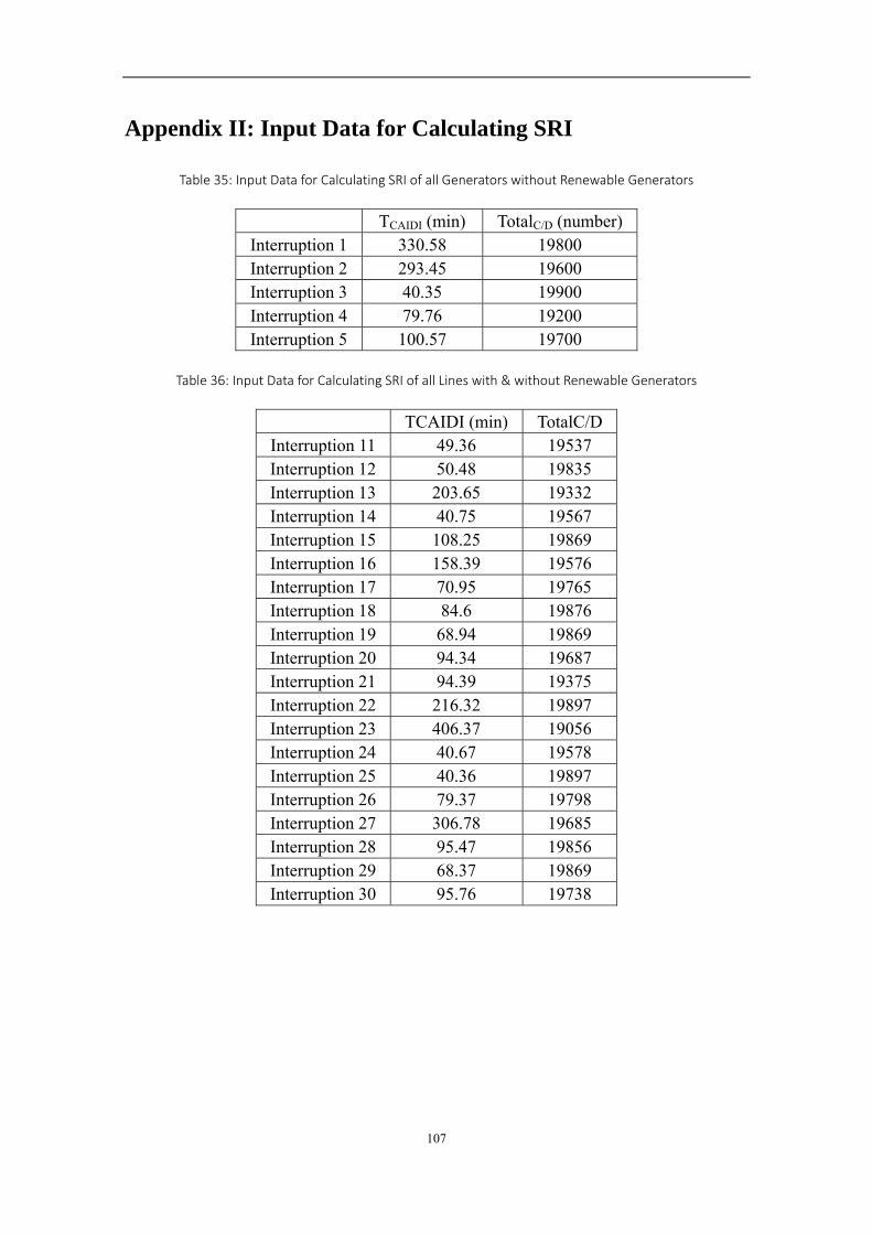
107
Appendix II: Input Data for Calculating SRI
Table 35: Input Data for Calculating SRI of all Generators without Renewable Generators
TCAIDI (min) TotalC/D (number) Interruption 1 330.58 19800 Interruption 2 293.45 19600 Interruption 3 40.35 19900 Interruption 4 79.76 19200 Interruption 5 100.57 19700
Table 36: Input Data for Calculating SRI of all Lines with & without Renewable Generators
TCAIDI (min) TotalC/D Interruption 11 49.36 19537 Interruption 12 50.48 19835 Interruption 13 203.65 19332 Interruption 14 40.75 19567 Interruption 15 108.25 19869 Interruption 16 158.39 19576 Interruption 17 70.95 19765 Interruption 18 84.6 19876 Interruption 19 68.94 19869 Interruption 20 94.34 19687 Interruption 21 94.39 19375 Interruption 22 216.32 19897 Interruption 23 406.37 19056 Interruption 24 40.67 19578 Interruption 25 40.36 19897 Interruption 26 79.37 19798 Interruption 27 306.78 19685 Interruption 28 95.47 19856 Interruption 29 68.37 19869 Interruption 30 95.76 19738
108
Appendix III: Simulation Results of Base Case
109
Appendix IV: Simulation Results of Sensitivity Simulation
Case 1

110
Appendix V: Simulation Results of Sensitivity Simulation
Case 2

TRITA TRITA-EE 2015:76
www.kth.se