Embed Size (px)
Citation preview
Ascential DataStage™ Enterprise MVS Edition
Mainframe Job TutorialVersion 7.5.1
Part No. 00D-028DS751
December 2004

This document, and the software described or referenced in it, are confidential and proprietary to Ascential
Software Corporation ("Ascential"). They are provided under, and are subject to, the terms and conditions of a
license agreement between Ascential and the licensee, and may not be transferred, disclosed, or otherwise
provided to third parties, unless otherwise permitted by that agreement. No portion of this publication may be
reproduced, stored in a retrieval system, or transmitted, in any form or by any means, electronic, mechanical,
photocopying, recording, or otherwise, without the prior written permission of Ascential. The specifications and
other information contained in this document for some purposes may not be complete, current, or correct, and are
subject to change without notice. NO REPRESENTATION OR OTHER AFFIRMATION OF FACT CONTAINED IN THIS
DOCUMENT, INCLUDING WITHOUT LIMITATION STATEMENTS REGARDING CAPACITY, PERFORMANCE, OR
SUITABILITY FOR USE OF PRODUCTS OR SOFTWARE DESCRIBED HEREIN, SHALL BE DEEMED TO BE A
WARRANTY BY ASCENTIAL FOR ANY PURPOSE OR GIVE RISE TO ANY LIABILITY OF ASCENTIAL WHATSOEVER.
THE SOFTWARE IS PROVIDED "AS IS", WITHOUT WARRANTY OF ANY KIND, EXPRESS OR IMPLIED, INCLUDING
BUT NOT LIMITED TO THE WARRANTIES OF MERCHANTABILITY, FITNESS FOR A PARTICULAR PURPOSE AND
NONINFRINGEMENT OF THIRD PARTY RIGHTS. IN NO EVENT SHALL ASCENTIAL BE LIABLE FOR ANY CLAIM, OR
ANY SPECIAL INDIRECT OR CONSEQUENTIAL DAMAGES, OR ANY DAMAGES WHATSOEVER RESULTING FROM
LOSS OF USE, DATA OR PROFITS, WHETHER IN AN ACTION OF CONTRACT, NEGLIGENCE OR OTHER TORTIOUS
ACTION, ARISING OUT OF OR IN CONNECTION WITH THE USE OR PERFORMANCE OF THIS SOFTWARE. If you
are acquiring this software on behalf of the U.S. government, the Government shall have only "Restricted Rights" in
the software and related documentation as defined in the Federal Acquisition Regulations (FARs) in Clause
52.227.19 (c) (2). If you are acquiring the software on behalf of the Department of Defense, the software shall be
classified as "Commercial Computer Software" and the Government shall have only "Restricted Rights" as defined
in Clause 252.227-7013 (c) (1) of DFARs.
© 2000-2004 Ascential Software Corporation. All rights reserved. DataStage®, EasyLogic®, EasyPath®, Enterprise
Data Quality Management®, Iterations®, Matchware®, Mercator®, MetaBroker®, Application Integration,
Simplified®, Ascential™, Ascential AuditStage™, Ascential DataStage™, Ascential ProfileStage™, Ascential
QualityStage™, Ascential Enterprise Integration Suite™, Ascential Real-time Integration Services™, Ascential
MetaStage™, and Ascential RTI™ are trademarks of Ascential Software Corporation or its affiliates and may be
registered in the United States or other jurisdictions.
The software delivered to Licensee may contain third-party software code. See Legal Notices (LegalNotices.pdf) for
more information.
How to Use this Guide
This manual describes the features of the Ascential DataStage™
Enterprise MVS Edition tool set and provides demonstrations of
simple data extractions and transformations in a mainframe data
warehouse environment. It is written for system administrators and
application developers who want to learn about Ascential DataStage
Enterprise MVS Edition and examine some typical usage examples.
If you are unfamiliar with data warehousing concepts, please read
Chapter 1 and Chapter 2 of Ascential DataStage Designer Guide for an
overview.
Note This tutorial demonstrates how to create and run
mainframe jobs, that is, jobs that run on mainframe
computers. You can also create jobs that run on a
DataStage server; these include server jobs and parallel
jobs. For more information about the different types of
DataStage jobs, refer to Ascential DataStage Server Job
Developer’s Guide, Ascential DataStage Mainframe Job
Developer’s Guide, and Ascential DataStage Parallel Job
Developer’s Guide.
This manual is organized by task. It begins with introductory
information and simple examples and progresses to more complex
tasks. It is not intended to replace formal Ascential DataStage training,
but rather to introduce you to the product and show you some of what
it can do. The tutorial CD contains the sample table definitions used in
this manual.
Welcome to the Mainframe Job TutorialThis tutorial takes you through some simple examples of extractions
and transformations in a mainframe data warehouse environment.
This introduces you to the functionality of DataStage mainframe jobs
and shows you how easy common data warehousing tasks can be,
with the right tools.
As you begin, you may find it helpful to start an Adobe Acrobat
Reader session in another window; you can then refer to the Ascential
Mainframe Job Tutorial iii
Before You Begin How to Use this Guide
DataStage documentation to see complete coverage of some of the
topics presented. For your convenience, we reference specific
sections in the Ascential DataStage documentation as we progress.
This document takes you through a demonstration of some of the
features of our tool. We cover the basics of:
Reading data from various mainframe sources
Designing job stages to model the flow of data into the warehouse
Defining constraints and column derivations
Merging, aggregating, and sorting data
Defining business rules
Calling external routines
Generating code and uploading jobs to a mainframe
We assume that you are familiar with fundamental database concepts
and terminology because you are working with our product. We also
assume that you have a basic understanding of mainframe computers
and the COBOL language since you are using Ascential DataStage
Enterprise MVS Edition. We cover a lot of material throughout the
demonstration process, and therefore we will not waste your time
with rudimentary explanations of concepts. If your database and
mainframe skills are advanced, some of what is covered may seem
like review. However, if you are new to databases or the mainframe
environment, you may want to consult an experienced user for
assistance with some of the exercises.
Before You BeginAscential DataStage Enterprise MVS Edition 7.5 must be installed. We
recommend that you install the DataStage server and client programs
on the same machine to keep the configuration as simple as possible,
but this is not essential.
As a mainframe computer is not always accessible, this tutorial is
written with the assumption that you are not connected to one. Not
having a mainframe will not hinder you in the use of this tutorial.
This tutorial will take you through the steps of generating code and
uploading a job, simulating what you would do on a mainframe, but
will not actually do it without the connection to a mainframe.
iv Mainframe Job Tutorial
How to Use this Guide How This Book is Organized
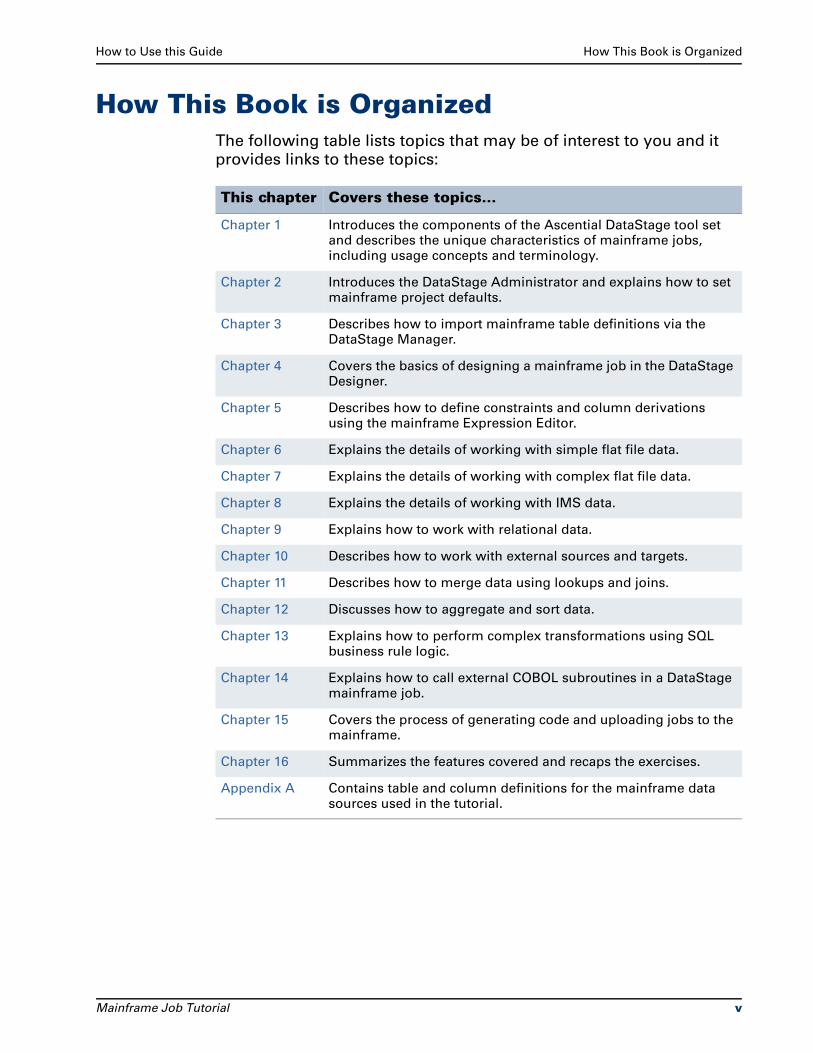
How This Book is OrganizedThe following table lists topics that may be of interest to you and it
provides links to these topics:
This chapter Covers these topics…
Chapter 1 Introduces the components of the Ascential DataStage tool set and describes the unique characteristics of mainframe jobs, including usage concepts and terminology.
Chapter 2 Introduces the DataStage Administrator and explains how to set mainframe project defaults.
Chapter 3 Describes how to import mainframe table definitions via the DataStage Manager.
Chapter 4 Covers the basics of designing a mainframe job in the DataStage Designer.
Chapter 5 Describes how to define constraints and column derivations using the mainframe Expression Editor.
Chapter 6 Explains the details of working with simple flat file data.
Chapter 7 Explains the details of working with complex flat file data.
Chapter 8 Explains the details of working with IMS data.
Chapter 9 Explains how to work with relational data.
Chapter 10 Describes how to work with external sources and targets.
Chapter 11 Describes how to merge data using lookups and joins.
Chapter 12 Discusses how to aggregate and sort data.
Chapter 13 Explains how to perform complex transformations using SQL business rule logic.
Chapter 14 Explains how to call external COBOL subroutines in a DataStage mainframe job.
Chapter 15 Covers the process of generating code and uploading jobs to the mainframe.
Chapter 16 Summarizes the features covered and recaps the exercises.
Appendix A Contains table and column definitions for the mainframe data sources used in the tutorial.
Mainframe Job Tutorial v
Related Documentation How to Use this Guide
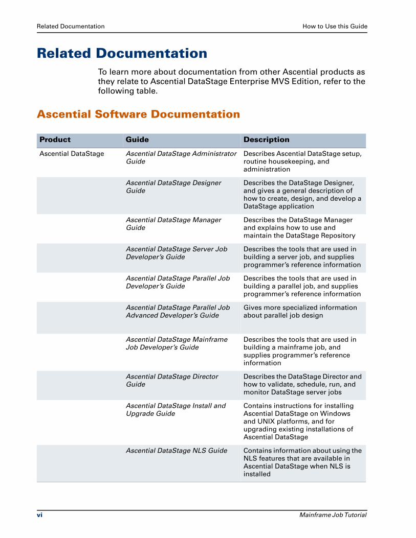
Related DocumentationTo learn more about documentation from other Ascential products as
they relate to Ascential DataStage Enterprise MVS Edition, refer to the
following table.
Ascential Software Documentation
Product Guide Description
Ascential DataStage Ascential DataStage Administrator Guide
Describes Ascential DataStage setup, routine housekeeping, and administration
Ascential DataStage Designer Guide
Describes the DataStage Designer, and gives a general description of how to create, design, and develop a DataStage application
Ascential DataStage Manager Guide
Describes the DataStage Manager and explains how to use and maintain the DataStage Repository
Ascential DataStage Server Job Developer’s Guide
Describes the tools that are used in building a server job, and supplies programmer’s reference information
Ascential DataStage Parallel Job Developer’s Guide
Describes the tools that are used in building a parallel job, and supplies programmer’s reference information
Ascential DataStage Parallel Job Advanced Developer’s Guide
Gives more specialized information about parallel job design
Ascential DataStage Mainframe Job Developer’s Guide
Describes the tools that are used in building a mainframe job, and supplies programmer’s reference information
Ascential DataStage Director Guide
Describes the DataStage Director and how to validate, schedule, run, and monitor DataStage server jobs
Ascential DataStage Install and Upgrade Guide
Contains instructions for installing Ascential DataStage on Windows and UNIX platforms, and for upgrading existing installations of Ascential DataStage
Ascential DataStage NLS Guide Contains information about using the NLS features that are available in Ascential DataStage when NLS is installed
vi Mainframe Job Tutorial
How to Use this Guide Documentation Conventions
These guides are also available online in PDF format. You can read
them with the Adobe Acrobat Reader supplied with Ascential
DataStage. See Ascential DataStage Install and Upgrade Guide for
details on installing the manuals and the Adobe Acrobat Reader.
You can use the Acrobat search facilities to search the whole Ascential
DataStage document set. To use this feature, select Edit Search
then choose the All PDF Documents in option and specify the
Ascential DataStage docs directory (by default this is C:\Program Files\ Ascential\DataStage\Docs).
Extensive online help is also supplied. This is especially useful when
you have become familiar with using Ascential DataStage and need to
look up particular pieces of information.
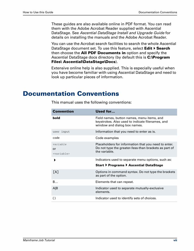
Documentation ConventionsThis manual uses the following conventions:
Convention Used for…
bold Field names, button names, menu items, and keystrokes. Also used to indicate filenames, and window and dialog box names.
user input Information that you need to enter as is.
code Code examples
variable
or
<variable>
Placeholders for information that you need to enter. Do not type the greater-/less-than brackets as part of the variable.
Indicators used to separate menu options, such as:
Start Programs Ascential DataStage
[A] Options in command syntax. Do not type the brackets as part of the option.
B… Elements that can repeat.
A|B Indicator used to separate mutually-exclusive elements.
{ } Indicator used to identify sets of choices.
Mainframe Job Tutorial vii
User Interface Conventions How to Use this Guide
The following conventions are also used:
Syntax definitions and examples are indented for ease in reading.
All punctuation marks included in the syntax—for example, commas, parentheses, or quotation marks—are required unless otherwise indicated.
Syntax lines that do not fit on one line in this manual are continued on subsequent lines. The continuation lines are indented. When entering syntax, type the entire syntax entry, including the continuation lines, on the same input line.
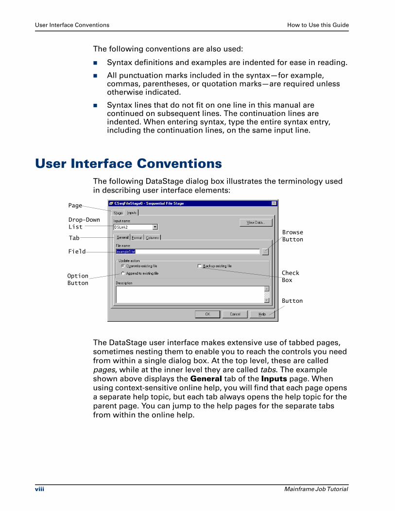
User Interface ConventionsThe following DataStage dialog box illustrates the terminology used
in describing user interface elements:
The DataStage user interface makes extensive use of tabbed pages,
sometimes nesting them to enable you to reach the controls you need
from within a single dialog box. At the top level, these are called
pages, while at the inner level they are called tabs. The example
shown above displays the General tab of the Inputs page. When
using context-sensitive online help, you will find that each page opens
a separate help topic, but each tab always opens the help topic for the
parent page. You can jump to the help pages for the separate tabs
from within the online help.
Browse Button
Check Box
Button
Drop-Down List
Tab
Field
Option Button
Page
viii Mainframe Job Tutorial
How to Use this Guide Contacting Support
Contacting SupportTo reach Customer Care, please refer to the information below:
Call toll-free: 1-866-INFONOW (1-866-463-6669)
Email: [email protected]
Ascential Developer Net: http://developernet.ascential.com
Please consult your support agreement for the location and
availability of customer support personnel.
To find the location and telephone number of the nearest Ascential
Software office outside of North America, please visit the Ascential
Software Corporation website at http://www.ascential.com.
Mainframe Job Tutorial ix
Contents
How to Use this GuideWelcome to the Mainframe Job Tutorial . . . . . . . . . . . . . . . . . . . . . . . . . . . . . . . iii
Before You Begin . . . . . . . . . . . . . . . . . . . . . . . . . . . . . . . . . . . . . . . . . . . . . . . . . . iv
How This Book is Organized . . . . . . . . . . . . . . . . . . . . . . . . . . . . . . . . . . . . . . . . . v
Related Documentation . . . . . . . . . . . . . . . . . . . . . . . . . . . . . . . . . . . . . . . . . . . . . vi
Ascential Software Documentation . . . . . . . . . . . . . . . . . . . . . . . . . . . . . . . . vi
Documentation Conventions . . . . . . . . . . . . . . . . . . . . . . . . . . . . . . . . . . . . . . . . vii
User Interface Conventions . . . . . . . . . . . . . . . . . . . . . . . . . . . . . . . . . . . . . . . . . viii
Contacting Support . . . . . . . . . . . . . . . . . . . . . . . . . . . . . . . . . . . . . . . . . . . . . . . . . ix
Chapter 1Introduction to DataStage Mainframe Jobs
Ascential DataStage Overview . . . . . . . . . . . . . . . . . . . . . . . . . . . . . . . . . . . . . . 1-1
Getting Started . . . . . . . . . . . . . . . . . . . . . . . . . . . . . . . . . . . . . . . . . . . . . . . . . . . 1-5
MVS Edition Terms and Concepts . . . . . . . . . . . . . . . . . . . . . . . . . . . . . . . . . . . 1-6
Chapter 2DataStage Administration
The DataStage Administrator . . . . . . . . . . . . . . . . . . . . . . . . . . . . . . . . . . . . . . . 2-1
Exercise 1: Set Project Defaults . . . . . . . . . . . . . . . . . . . . . . . . . . . . . . . . . . . . . 2-1
Summary . . . . . . . . . . . . . . . . . . . . . . . . . . . . . . . . . . . . . . . . . . . . . . . . . . . . . . . 2-5
Chapter 3Importing Table Definitions
The DataStage Manager . . . . . . . . . . . . . . . . . . . . . . . . . . . . . . . . . . . . . . . . . . . 3-1
Exercise 2: Import Mainframe Table Definitions . . . . . . . . . . . . . . . . . . . . . . . . 3-4
Summary . . . . . . . . . . . . . . . . . . . . . . . . . . . . . . . . . . . . . . . . . . . . . . . . . . . . . . . 3-8
Mainframe Job Tutorial xi
Contents
Chapter 4Designing a Mainframe Job
The DataStage Designer . . . . . . . . . . . . . . . . . . . . . . . . . . . . . . . . . . . . . . . . . . . 4-1
Exercise 3: Specify Designer Options . . . . . . . . . . . . . . . . . . . . . . . . . . . . . . . . 4-7
Exercise 4: Create a Mainframe Job. . . . . . . . . . . . . . . . . . . . . . . . . . . . . . . . . . 4-9
Summary . . . . . . . . . . . . . . . . . . . . . . . . . . . . . . . . . . . . . . . . . . . . . . . . . . . . . . 4-21
Chapter 5Defining Constraints and Derivations
Exercise 5: Define a Constraint . . . . . . . . . . . . . . . . . . . . . . . . . . . . . . . . . . . . . . 5-1
Exercise 6: Define a Stage Variable . . . . . . . . . . . . . . . . . . . . . . . . . . . . . . . . . . 5-7
Exercise 7: Define a Job Parameter . . . . . . . . . . . . . . . . . . . . . . . . . . . . . . . . . 5-10
Summary . . . . . . . . . . . . . . . . . . . . . . . . . . . . . . . . . . . . . . . . . . . . . . . . . . . . . . 5-13
Chapter 6Working with Simple Flat Files
Simple Flat File Stage Types. . . . . . . . . . . . . . . . . . . . . . . . . . . . . . . . . . . . . . . . 6-1
Exercise 8: Read Delimited Flat File Data. . . . . . . . . . . . . . . . . . . . . . . . . . . . . . 6-3
Exercise 9: Write Data to a DB2 Load Ready File . . . . . . . . . . . . . . . . . . . . . . . 6-9
Exercise 10: Use an FTP Stage . . . . . . . . . . . . . . . . . . . . . . . . . . . . . . . . . . . . . 6-12
Summary . . . . . . . . . . . . . . . . . . . . . . . . . . . . . . . . . . . . . . . . . . . . . . . . . . . . . . 6-14
Chapter 7Working with Complex Flat Files
Complex Flat File Stage Types . . . . . . . . . . . . . . . . . . . . . . . . . . . . . . . . . . . . . . 7-2
Exercise 11: Use a Complex Flat File Stage. . . . . . . . . . . . . . . . . . . . . . . . . . . . 7-3
Exercise 12: Flatten an Array . . . . . . . . . . . . . . . . . . . . . . . . . . . . . . . . . . . . . . . 7-6
Exercise 13: Work with an ODO Clause . . . . . . . . . . . . . . . . . . . . . . . . . . . . . . . 7-8
Exercise 14: Use a Multi-Format Flat File Stage . . . . . . . . . . . . . . . . . . . . . . . 7-12
Exercise 15: Merge Multi-Format Record Types . . . . . . . . . . . . . . . . . . . . . . . 7-17
Summary . . . . . . . . . . . . . . . . . . . . . . . . . . . . . . . . . . . . . . . . . . . . . . . . . . . . . . 7-18
Chapter 8Working with IMS Data
Exercise 16: Import IMS Definitions. . . . . . . . . . . . . . . . . . . . . . . . . . . . . . . . . . 8-1
Exercise 17: Read Data from an IMS Source . . . . . . . . . . . . . . . . . . . . . . . . . . . 8-6
Summary . . . . . . . . . . . . . . . . . . . . . . . . . . . . . . . . . . . . . . . . . . . . . . . . . . . . . . . 8-9
xii Mainframe Job Tutorial
Contents
Chapter 9Working with Relational Data
Relational Stages . . . . . . . . . . . . . . . . . . . . . . . . . . . . . . . . . . . . . . . . . . . . . . . . . 9-1
Exercise 18: Read Data from a Relational Source . . . . . . . . . . . . . . . . . . . . . . . 9-2
Exercise 19: Write Data to a Relational Target . . . . . . . . . . . . . . . . . . . . . . . . . 9-5
Summary . . . . . . . . . . . . . . . . . . . . . . . . . . . . . . . . . . . . . . . . . . . . . . . . . . . . . . . 9-8
Chapter 10Working with External Sources and Targets
Exercise 20: Read Data From an External Source . . . . . . . . . . . . . . . . . . . . . . 10-2
Exercise 21: Write Data to an External Target . . . . . . . . . . . . . . . . . . . . . . . . . 10-6
Summary . . . . . . . . . . . . . . . . . . . . . . . . . . . . . . . . . . . . . . . . . . . . . . . . . . . . . . 10-8
Chapter 11Merging Data Using Joins and Lookups
Exercise 22: Merge Data Using a Join Stage. . . . . . . . . . . . . . . . . . . . . . . . . . 11-2
Exercise 23: Merge Data Using a Lookup Stage . . . . . . . . . . . . . . . . . . . . . . . 11-5
Summary . . . . . . . . . . . . . . . . . . . . . . . . . . . . . . . . . . . . . . . . . . . . . . . . . . . . . . 11-9
Chapter 12Sorting and Aggregating Data
Exercise 24: Sort Data . . . . . . . . . . . . . . . . . . . . . . . . . . . . . . . . . . . . . . . . . . . . 12-2
Exercise 25: Aggregate Data . . . . . . . . . . . . . . . . . . . . . . . . . . . . . . . . . . . . . . . 12-3
Exercise 26: Use ENDOFDATA . . . . . . . . . . . . . . . . . . . . . . . . . . . . . . . . . . . . . 12-6
Summary . . . . . . . . . . . . . . . . . . . . . . . . . . . . . . . . . . . . . . . . . . . . . . . . . . . . . . 12-9
Chapter 13Defining Business Rules
Exercise 27: Controlling Relational Transactions . . . . . . . . . . . . . . . . . . . . . . 13-1
Summary . . . . . . . . . . . . . . . . . . . . . . . . . . . . . . . . . . . . . . . . . . . . . . . . . . . . . . 13-5
Chapter 14Calling External Routines
Exercise 28: Define Routine Meta Data . . . . . . . . . . . . . . . . . . . . . . . . . . . . . . 14-1
Exercise 29: Call an External Routine . . . . . . . . . . . . . . . . . . . . . . . . . . . . . . . . 14-2
Summary . . . . . . . . . . . . . . . . . . . . . . . . . . . . . . . . . . . . . . . . . . . . . . . . . . . . . . 14-7
Mainframe Job Tutorial xiii
Contents
Chapter 15Generating Code
Exercise 30: Modify JCL Templates . . . . . . . . . . . . . . . . . . . . . . . . . . . . . . . . . 15-1
Exercise 31: Validate a Job and Generate Code . . . . . . . . . . . . . . . . . . . . . . . 15-3
Exercise 32: Define a Machine Profile . . . . . . . . . . . . . . . . . . . . . . . . . . . . . . . 15-4
Exercise 33: Upload a Job. . . . . . . . . . . . . . . . . . . . . . . . . . . . . . . . . . . . . . . . . 15-6
Summary . . . . . . . . . . . . . . . . . . . . . . . . . . . . . . . . . . . . . . . . . . . . . . . . . . . . . . 15-7
Chapter 16Summary
Main Features in Ascential DataStage Enterprise MVS Edition. . . . . . . . . . . 16-1
Recap of the Exercises. . . . . . . . . . . . . . . . . . . . . . . . . . . . . . . . . . . . . . . . . . . . 16-2
Contacting Ascential Software Corporation . . . . . . . . . . . . . . . . . . . . . . . . . . 16-4
Appendix ASample Data Definitions
COBOL File Definitions . . . . . . . . . . . . . . . . . . . . . . . . . . . . . . . . . . . . . . . . . . . . A-2
DB2 DCLGen File Definitions . . . . . . . . . . . . . . . . . . . . . . . . . . . . . . . . . . . . . . . A-4
IMS Definitions. . . . . . . . . . . . . . . . . . . . . . . . . . . . . . . . . . . . . . . . . . . . . . . . . . . A-5
Index
xiv Mainframe Job Tutorial
1Introduction to DataStage
Mainframe Jobs
This tutorial describes how to design and develop DataStage
mainframe jobs. If you have Ascential DataStage Enterprise MVS
Edition installed, you can generate jobs that are compiled and run on
a mainframe. Data read by these jobs is then loaded into a data
warehouse.
This chapter gives a general introduction to Ascential DataStage and
its components and describes the unique characteristics of mainframe
jobs. If you have already completed the server job tutorial, some of
this will be a review.
Ascential DataStage OverviewAscential DataStage enables you to quickly build a data warehouse or
data mart. It is an integrated set of tools for designing and developing
applications that extract data from one or more data sources, perform
complex transformations of the data, and load one or more target files
or databases with the resulting data.
Solutions developed with Ascential DataStage are open and scalable;
you can, for example, readily add data sources and targets or handle
increased volumes of data.
Mainframe Job Tutorial 1-1
Ascential DataStage Overview Introduction to DataStage Mainframe Jobs
Server ComponentsAscential DataStage has three server components:
Repository. A central store that contains all the information required to build a data mart or data warehouse.
DataStage Server. Runs executable server jobs, under the control of the DataStage Director, that extract, transform, and load data into a data warehouse.
DataStage Package Installer. A user interface used to install packaged DataStage jobs and plug-ins.
Client ComponentsAscential DataStage has four client components, which are installed
on any PC running Windows 2000, Windows NT 4.0, or Windows XP
Professional:
DataStage Manager. A user interface used to view and edit the contents of the Repository.
DataStage Designer. A graphical tool used to create DataStage server, mainframe, and parallel jobs.
DataStage Administrator. A user interface used to perform basic configuration tasks such as setting up users, creating and deleting projects, and setting project properties.
DataStage Director. A user interface used to validate, schedule, run, and monitor DataStage server jobs. The Director is not used in mainframe jobs.
The DataStage Manager, Designer, and Administrator are introduced
during the mainframe tutorial exercises. You learn how to use these
tools to accomplish specific tasks and, in doing so, you gain some
familiarity with the capabilities they provide.
The server components require little interaction, although the
exercises in which you use the DataStage Manager also give you the
opportunity to examine the Repository.
ProjectsIn Ascential DataStage, all development work is done in a project.
Projects are created during the installation process. After installation,
new projects can be added using the DataStage Administrator.
1-2 Mainframe Job Tutorial
Introduction to DataStage Mainframe Jobs Ascential DataStage Overview
Whenever you start a DataStage client, you are prompted to attach to
a DataStage project. Each project may contain:
DataStage jobs. A set of jobs for loading and maintaining a data warehouse. There is no limit to the number of jobs you can create in a project.
Built-in components. Predefined components used in a job.
User-defined components. Customized components created using the DataStage Manager. Each user-defined component performs a specific task in a job.
JobsDataStage jobs consist of individual stages, linked together to
represent the flow of data from one or more data sources into a data
warehouse. Each stage describes a particular database or process. For
example, one stage may extract data from a data source, while
another transforms it. Stages are added to a job and linked together
using the Designer.
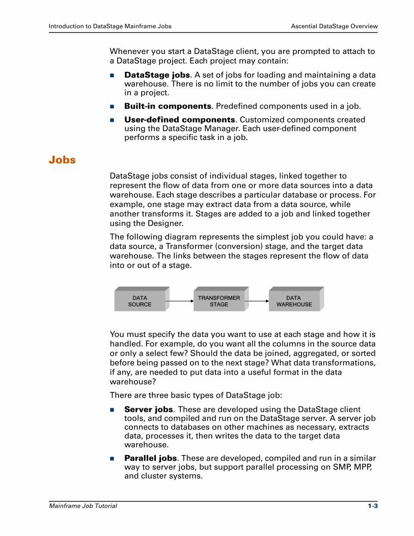
The following diagram represents the simplest job you could have: a
data source, a Transformer (conversion) stage, and the target data
warehouse. The links between the stages represent the flow of data
into or out of a stage.
You must specify the data you want to use at each stage and how it is
handled. For example, do you want all the columns in the source data
or only a select few? Should the data be joined, aggregated, or sorted
before being passed on to the next stage? What data transformations,
if any, are needed to put data into a useful format in the data
warehouse?
There are three basic types of DataStage job:
Server jobs. These are developed using the DataStage client tools, and compiled and run on the DataStage server. A server job connects to databases on other machines as necessary, extracts data, processes it, then writes the data to the target data warehouse.
Parallel jobs. These are developed, compiled and run in a similar way to server jobs, but support parallel processing on SMP, MPP, and cluster systems.
DATASOURCE
TRANSFORMERSTAGE
DATA WAREHOUSE
DATASOURCE
TRANSFORMERSTAGE
DATA WAREHOUSE
Mainframe Job Tutorial 1-3
Ascential DataStage Overview Introduction to DataStage Mainframe Jobs
Mainframe jobs. These are developed using the same DataStage client tools as for server and parallel jobs, but are compiled and run on a mainframe. The Designer generates a COBOL source file and supporting JCL script, which you upload to the target mainframe computer. The job is then compiled and run on the mainframe under the control of native mainframe software. Data extracted by mainframe jobs is then loaded into the data warehouse.
For more information about server, parallel, and mainframe jobs, refer
to Ascential DataStage Server Job Developer’s Guide, Ascential
DataStage Parallel Job Developer’s Guide, and Ascential DataStage
Mainframe Job Developer’s Guide.
StagesA stage can be passive or active. Passive stages handle access to files
and tables for the extraction and writing of data. Active stages model
the flow of data and provide mechanisms for combining data streams,
aggregating data, and converting data from one data type to another.
A stage usually has at least one data input and one data output.
However, some stages can accept more than one data input and can
output to more than one stage. The properties of each stage and the
data on each input and output link are specified using a stage editor.
There are four stage types in mainframe jobs:
Source stages. Used to read data from a data source. Mainframe source stage types include:
– Complex Flat File
– Delimited Flat File (can also be used as a target stage)
– External Source
– Fixed-Width Flat File (can also be used as a target stage)
– IMS
– Multi-Format Flat File
– Relational (can also be used as a target stage)
– Teradata Export
– Teradata Relational (can also be used as a target stage)
Target stages. Used to write data to a target data warehouse. Mainframe target stage types include:
– DB2 Load Ready Flat File
– Delimited Flat File (can also be used as a source stage)
1-4 Mainframe Job Tutorial
Introduction to DataStage Mainframe Jobs Getting Started
– External Target
– Fixed-Width Flat File (can also be used as a source stage)
– Relational (can also be used as a source stage)
– Teradata Load
– Teradata Relational (can also be used as a source stage)
Processing stages. Used to transform data before writing it to the target. Mainframe processing stage types include:
– Aggregator
– Business Rule
– External Routine
– Join
– Link Collector
– Lookup
– Sort
– Transformer
Post-processing stage. Used to post-process target files produced by a mainframe job. There is one type of post-processing stage:
– FTP
These stage types are described in more detail in Chapter 4.
Getting StartedThis tutorial is designed to familiarize you with the features and
functionality in DataStage mainframe jobs. As you work through the
tutorial exercises, you create jobs that read data, transform it, then
load it into target files or tables. You need not have an active
mainframe connection to complete the tutorial, as final job upload is
simulated.
At the end of this tutorial, you will understand how to:
Attach to a project and specify project defaults for mainframe jobs in the DataStage Administrator
Import meta data from mainframe sources in the DataStage Manager
Design a mainframe job in the DataStage Designer
Mainframe Job Tutorial 1-5
MVS Edition Terms and Concepts Introduction to DataStage Mainframe Jobs
Define constraints and output column derivations using the mainframe Expression Editor
Read data from and write data to different types of flat files
Read data from IMS databases
Read data from and write data to relational tables
Read data from external sources and write data to external targets
Define table lookups and joins
Define aggregations and sorts
Define complex data transformations using SQL business rule logic
Define and call external COBOL routines
Generate COBOL source code and compile and run JCL
Upload generated files to a mainframe
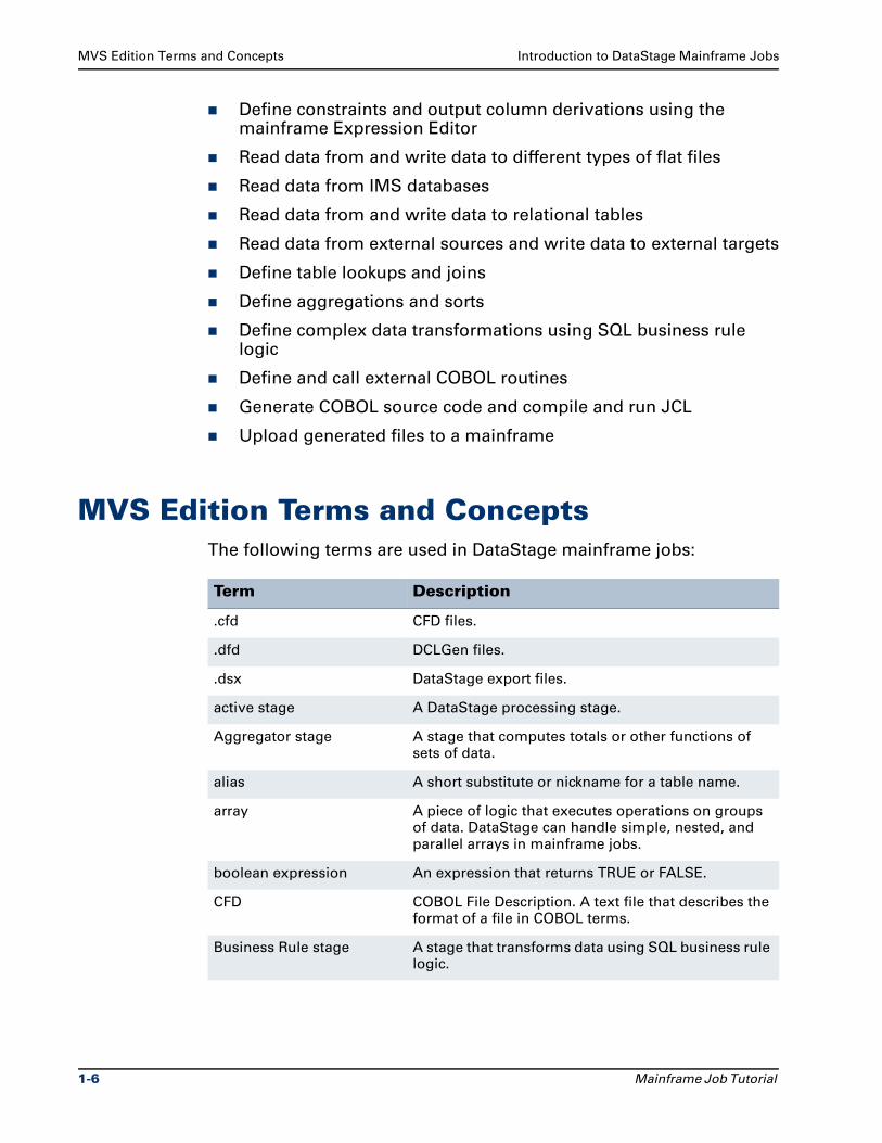
MVS Edition Terms and ConceptsThe following terms are used in DataStage mainframe jobs:
Term Description
.cfd CFD files.
.dfd DCLGen files.
.dsx DataStage export files.
active stage A DataStage processing stage.
Aggregator stage A stage that computes totals or other functions of sets of data.
alias A short substitute or nickname for a table name.
array A piece of logic that executes operations on groups of data. DataStage can handle simple, nested, and parallel arrays in mainframe jobs.
boolean expression An expression that returns TRUE or FALSE.
CFD COBOL File Description. A text file that describes the format of a file in COBOL terms.
Business Rule stage A stage that transforms data using SQL business rule logic.
1-6 Mainframe Job Tutorial
Introduction to DataStage Mainframe Jobs MVS Edition Terms and Concepts
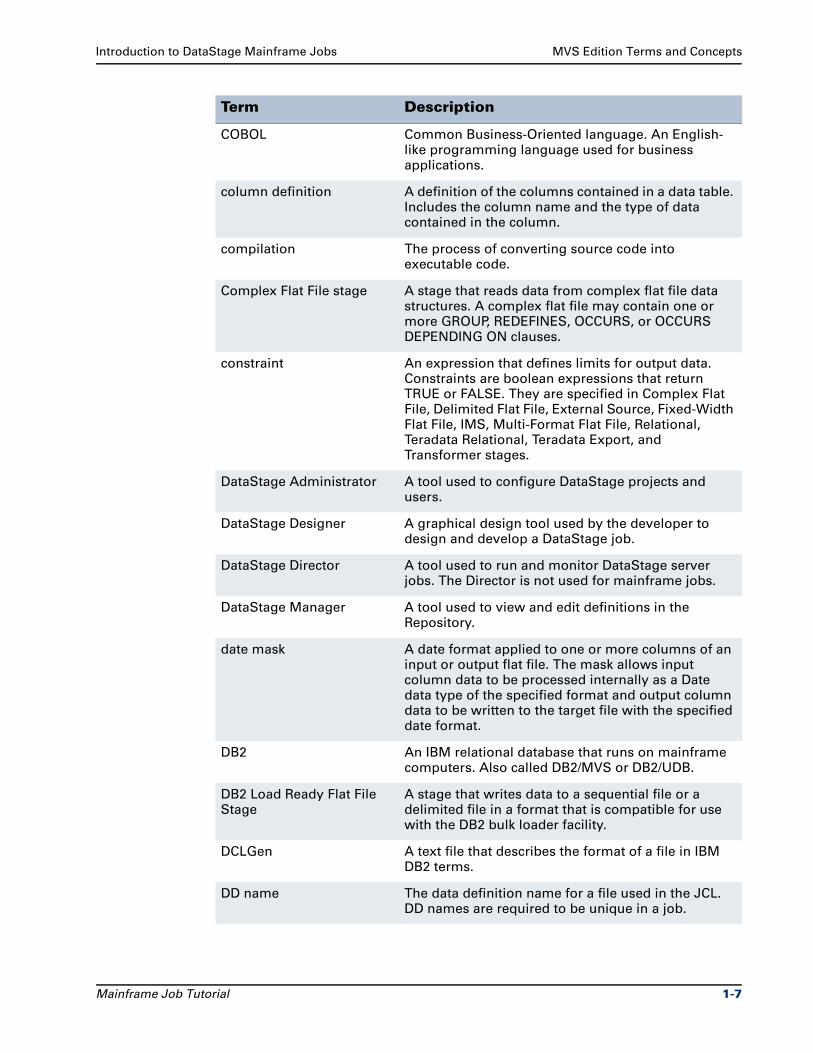
COBOL Common Business-Oriented language. An English-like programming language used for business applications.
column definition A definition of the columns contained in a data table. Includes the column name and the type of data contained in the column.
compilation The process of converting source code into executable code.
Complex Flat File stage A stage that reads data from complex flat file data structures. A complex flat file may contain one or more GROUP, REDEFINES, OCCURS, or OCCURS DEPENDING ON clauses.
constraint An expression that defines limits for output data. Constraints are boolean expressions that return TRUE or FALSE. They are specified in Complex Flat File, Delimited Flat File, External Source, Fixed-Width Flat File, IMS, Multi-Format Flat File, Relational, Teradata Relational, Teradata Export, and Transformer stages.
DataStage Administrator A tool used to configure DataStage projects and users.
DataStage Designer A graphical design tool used by the developer to design and develop a DataStage job.
DataStage Director A tool used to run and monitor DataStage server jobs. The Director is not used for mainframe jobs.
DataStage Manager A tool used to view and edit definitions in the Repository.
date mask A date format applied to one or more columns of an input or output flat file. The mask allows input column data to be processed internally as a Date data type of the specified format and output column data to be written to the target file with the specified date format.
DB2 An IBM relational database that runs on mainframe computers. Also called DB2/MVS or DB2/UDB.
DB2 Load Ready Flat File Stage
A stage that writes data to a sequential file or a delimited file in a format that is compatible for use with the DB2 bulk loader facility.
DCLGen A text file that describes the format of a file in IBM DB2 terms.
DD name The data definition name for a file used in the JCL. DD names are required to be unique in a job.
Term Description
Mainframe Job Tutorial 1-7
MVS Edition Terms and Concepts Introduction to DataStage Mainframe Jobs
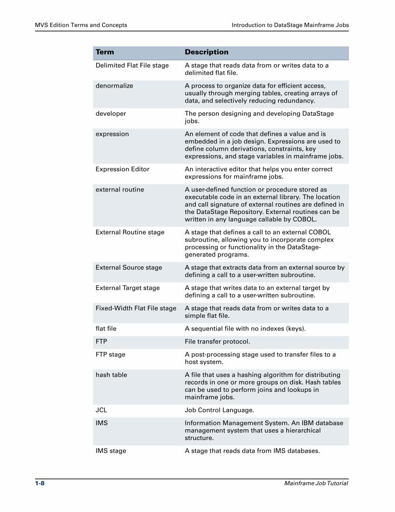
Delimited Flat File stage A stage that reads data from or writes data to a delimited flat file.
denormalize A process to organize data for efficient access, usually through merging tables, creating arrays of data, and selectively reducing redundancy.
developer The person designing and developing DataStage jobs.
expression An element of code that defines a value and is embedded in a job design. Expressions are used to define column derivations, constraints, key expressions, and stage variables in mainframe jobs.
Expression Editor An interactive editor that helps you enter correct expressions for mainframe jobs.
external routine A user-defined function or procedure stored as executable code in an external library. The location and call signature of external routines are defined in the DataStage Repository. External routines can be written in any language callable by COBOL.
External Routine stage A stage that defines a call to an external COBOL subroutine, allowing you to incorporate complex processing or functionality in the DataStage-generated programs.
External Source stage A stage that extracts data from an external source by defining a call to a user-written subroutine.
External Target stage A stage that writes data to an external target by defining a call to a user-written subroutine.
Fixed-Width Flat File stage A stage that reads data from or writes data to a simple flat file.
flat file A sequential file with no indexes (keys).
FTP File transfer protocol.
FTP stage A post-processing stage used to transfer files to a host system.
hash table A file that uses a hashing algorithm for distributing records in one or more groups on disk. Hash tables can be used to perform joins and lookups in mainframe jobs.
JCL Job Control Language.
IMS Information Management System. An IBM database management system that uses a hierarchical structure.
IMS stage A stage that reads data from IMS databases.
Term Description
1-8 Mainframe Job Tutorial
Introduction to DataStage Mainframe Jobs MVS Edition Terms and Concepts
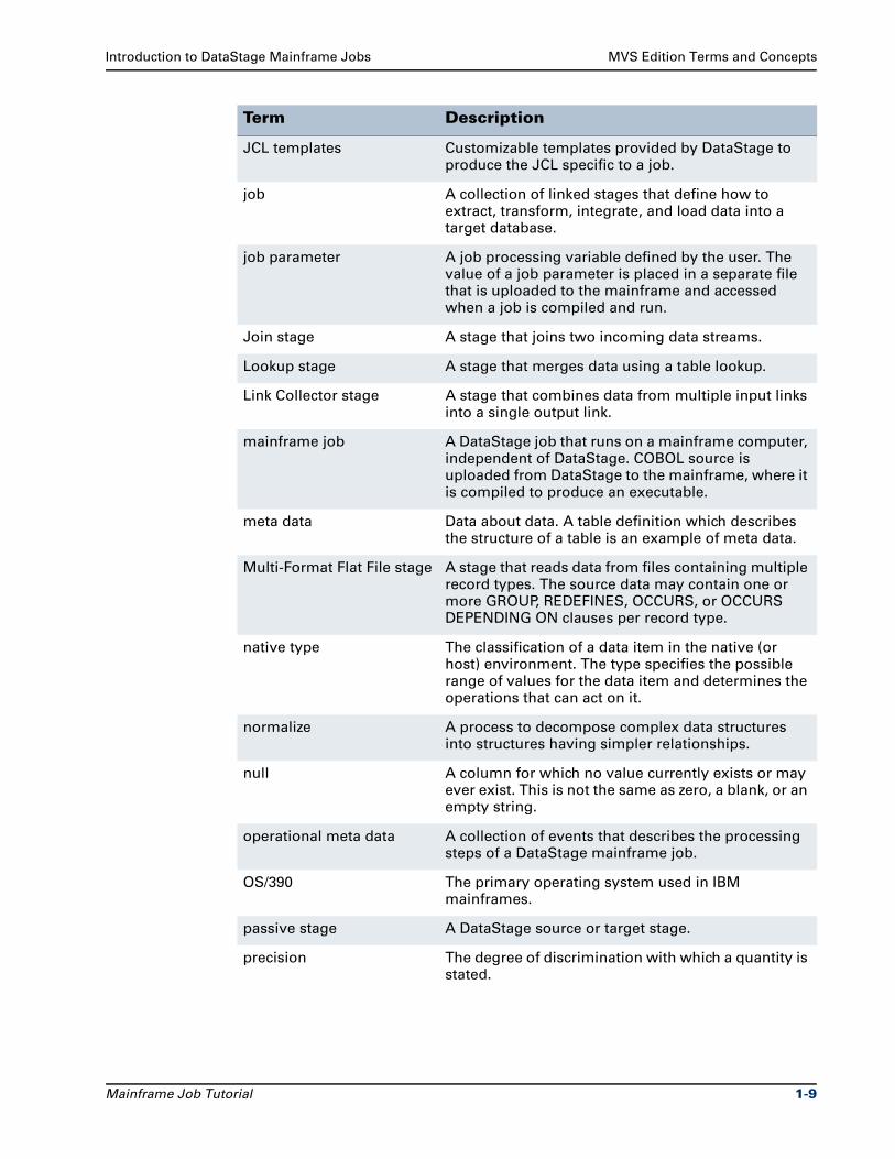
JCL templates Customizable templates provided by DataStage to produce the JCL specific to a job.
job A collection of linked stages that define how to extract, transform, integrate, and load data into a target database.
job parameter A job processing variable defined by the user. The value of a job parameter is placed in a separate file that is uploaded to the mainframe and accessed when a job is compiled and run.
Join stage A stage that joins two incoming data streams.
Lookup stage A stage that merges data using a table lookup.
Link Collector stage A stage that combines data from multiple input links into a single output link.
mainframe job A DataStage job that runs on a mainframe computer, independent of DataStage. COBOL source is uploaded from DataStage to the mainframe, where it is compiled to produce an executable.
meta data Data about data. A table definition which describes the structure of a table is an example of meta data.
Multi-Format Flat File stage A stage that reads data from files containing multiple record types. The source data may contain one or more GROUP, REDEFINES, OCCURS, or OCCURS DEPENDING ON clauses per record type.
native type The classification of a data item in the native (or host) environment. The type specifies the possible range of values for the data item and determines the operations that can act on it.
normalize A process to decompose complex data structures into structures having simpler relationships.
null A column for which no value currently exists or may ever exist. This is not the same as zero, a blank, or an empty string.
operational meta data A collection of events that describes the processing steps of a DataStage mainframe job.
OS/390 The primary operating system used in IBM mainframes.
passive stage A DataStage source or target stage.
precision The degree of discrimination with which a quantity is stated.
Term Description
Mainframe Job Tutorial 1-9
MVS Edition Terms and Concepts Introduction to DataStage Mainframe Jobs
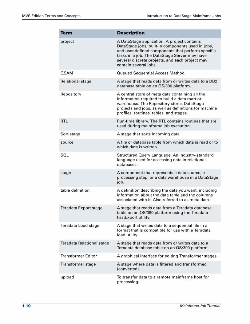
project A DataStage application. A project contains DataStage jobs, built-in components used in jobs, and user-defined components that perform specific tasks in a job. The DataStage Server may have several discrete projects, and each project may contain several jobs.
QSAM Queued Sequential Access Method.
Relational stage A stage that reads data from or writes data to a DB2 database table on an OS/390 platform.
Repository A central store of meta data containing all the information required to build a data mart or warehouse. The Repository stores DataStage projects and jobs, as well as definitions for machine profiles, routines, tables, and stages.
RTL Run-time library. The RTL contains routines that are used during mainframe job execution.
Sort stage A stage that sorts incoming data.
source A file or database table from which data is read or to which data is written.
SQL Structured Query Language. An industry-standard language used for accessing data in relational databases.
stage A component that represents a data source, a processing step, or a data warehouse in a DataStage job.
table definition A definition describing the data you want, including information about the data table and the columns associated with it. Also referred to as meta data.
Teradata Export stage A stage that reads data from a Teradata database table on an OS/390 platform using the Teradata FastExport utility.
Teradata Load stage A stage that writes data to a sequential file in a format that is compatible for use with a Teradata load utility.
Teradata Relational stage A stage that reads data from or writes data to a Teradata database table on an OS/390 platform.
Transformer Editor A graphical interface for editing Transformer stages.
Transformer stage A stage where data is filtered and transformed (converted).
upload To transfer data to a remote mainframe host for processing.
Term Description
1-10 Mainframe Job Tutorial
Introduction to DataStage Mainframe Jobs MVS Edition Terms and Concepts
variable-block file A complex flat file that contains variable record lengths.
VSAM Virtual Storage Access Method. A file management system for IBM’s MVS operating system.
Term Description
Mainframe Job Tutorial 1-11
2DataStage Administration
This chapter familiarizes you with the basics of the DataStage
Administrator. You learn how to attach to DataStage and set project
defaults for mainframe jobs.
The DataStage AdministratorIn mainframe jobs the DataStage Administrator is used to:
Change license details
Set up DataStage users
Add, delete, and move DataStage projects
Clean up project files
Set the timeout interval on the server computer
View and edit project properties
Some of these tasks require specific administration rights and are
usually performed by a system administrator. Others are basic
configuration tasks that any DataStage developer can perform. For
detailed information about the features of the DataStage
Administrator, refer to Ascential DataStage Administrator Guide.
Exercise 1: Set Project DefaultsBefore you design jobs in Ascential DataStage, you need to perform a
few steps in the Administrator. This exercise shows you how to attach
to DataStage and specify mainframe project defaults.
Mainframe Job Tutorial 2-1
Exercise 1: Set Project Defaults DataStage Administration
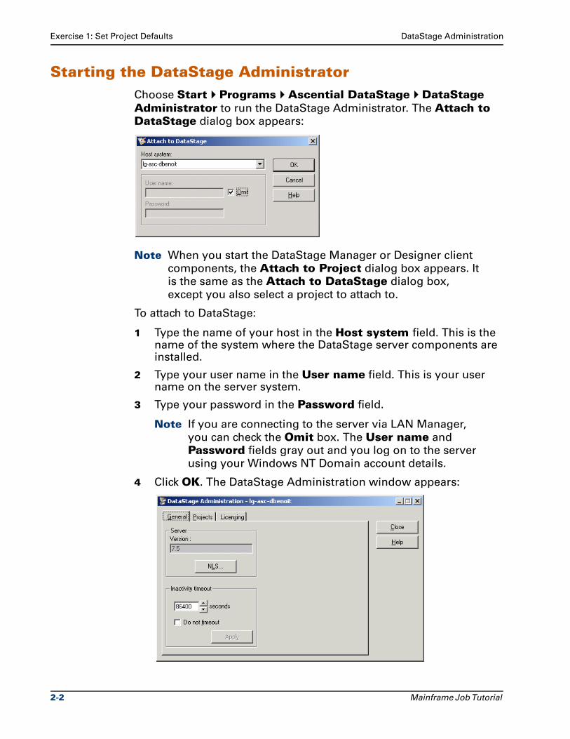
Starting the DataStage AdministratorChoose Start Programs Ascential DataStage DataStage Administrator to run the DataStage Administrator. The Attach to DataStage dialog box appears:
Note When you start the DataStage Manager or Designer client
components, the Attach to Project dialog box appears. It
is the same as the Attach to DataStage dialog box,
except you also select a project to attach to.
To attach to DataStage:
1 Type the name of your host in the Host system field. This is the name of the system where the DataStage server components are installed.
2 Type your user name in the User name field. This is your user name on the server system.
3 Type your password in the Password field.
Note If you are connecting to the server via LAN Manager,
you can check the Omit box. The User name and
Password fields gray out and you log on to the server
using your Windows NT Domain account details.
4 Click OK. The DataStage Administration window appears:
2-2 Mainframe Job Tutorial
DataStage Administration Exercise 1: Set Project Defaults
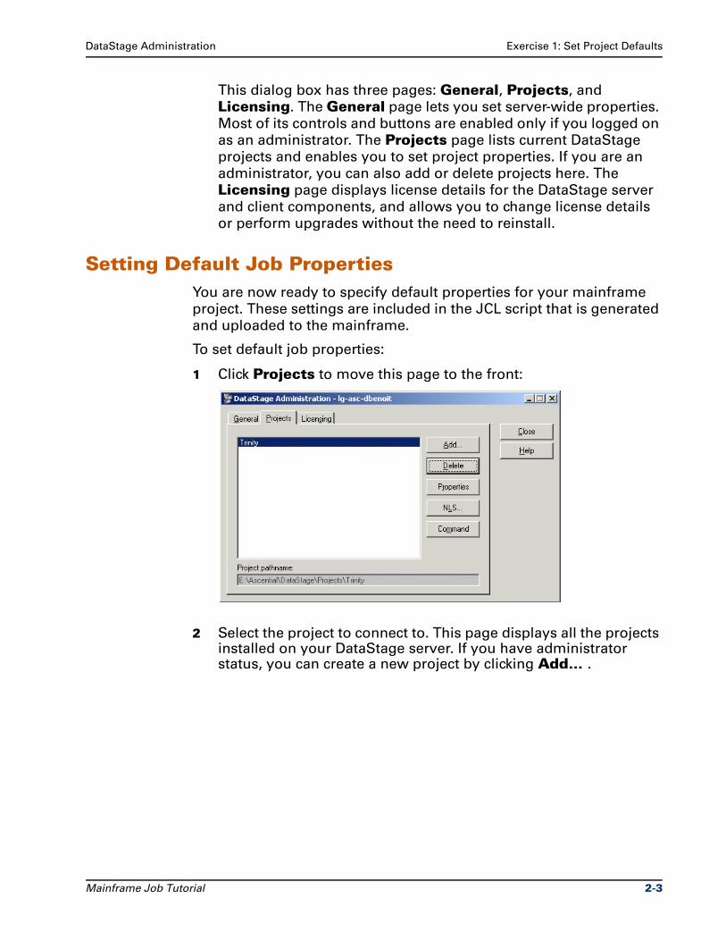
This dialog box has three pages: General, Projects, and
Licensing. The General page lets you set server-wide properties.
Most of its controls and buttons are enabled only if you logged on
as an administrator. The Projects page lists current DataStage
projects and enables you to set project properties. If you are an
administrator, you can also add or delete projects here. The
Licensing page displays license details for the DataStage server
and client components, and allows you to change license details
or perform upgrades without the need to reinstall.
Setting Default Job PropertiesYou are now ready to specify default properties for your mainframe
project. These settings are included in the JCL script that is generated
and uploaded to the mainframe.
To set default job properties:
1 Click Projects to move this page to the front:
2 Select the project to connect to. This page displays all the projects installed on your DataStage server. If you have administrator status, you can create a new project by clicking Add… .
Mainframe Job Tutorial 2-3
Exercise 1: Set Project Defaults DataStage Administration
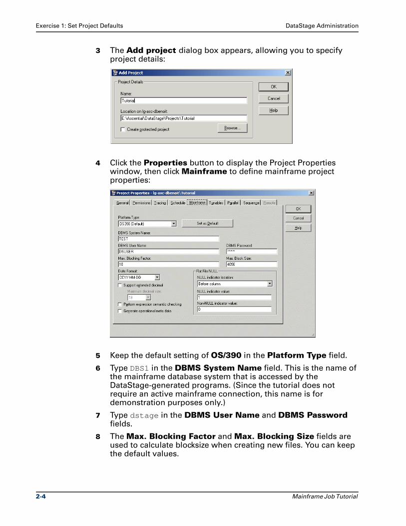
3 The Add project dialog box appears, allowing you to specify project details:
4 Click the Properties button to display the Project Properties window, then click Mainframe to define mainframe project properties:
5 Keep the default setting of OS/390 in the Platform Type field.
6 Type DBS1 in the DBMS System Name field. This is the name of the mainframe database system that is accessed by the DataStage-generated programs. (Since the tutorial does not require an active mainframe connection, this name is for demonstration purposes only.)
7 Type dstage in the DBMS User Name and DBMS Password fields.
8 The Max. Blocking Factor and Max. Blocking Size fields are used to calculate blocksize when creating new files. You can keep the default values.
2-4 Mainframe Job Tutorial
DataStage Administration Summary
9 Keep the default setting of CCYY-MM-DD in the Date Format drop-down list. This field allows you to specify, at the project level, the format of a DATE field that is retrieved from or written to a DB2 table. You can override this date format at the job level, as you will see in a later exercise.
10 Select the Support extended decimal check box and select 31 in the Maximum decimal size drop-down box. This enables DataStage to support Decimal columns with length up to 31. The default maximum size is 18.
11 Notice the next two check boxes: Perform expression semantic checking and Generate operational meta data. The first option enables semantic checking in the mainframe Expression Editor. The second option captures meta data about the processing steps of a mainframe job, which can then be used in Ascential MetaStage™. You can select either of these options at the project level or the job level. Keep the default settings here; you will learn more about these options later in the exercises.
12 Look over the Flat File NULL area. These fields allow you to specify the location of NULL indicators in flat file column definitions, along with the characters used to indicate nullability. These settings can be specified at either the project level or the job level. Keep the default settings here.
13 Click OK. Once you have returned to the DataStage Administration window, click Close to exit the DataStage Administrator.
SummaryIn this chapter you logged on to the DataStage Administrator, selected
a project, and defined default project properties. You became familiar
with the mainframe project settings that are used during job design,
code generation, and job upload.
Next, you use the DataStage Manager to import mainframe table
definitions.
Mainframe Job Tutorial 2-5
3Importing Table Definitions
Before you design a DataStage job, you need to create meta data for
your mainframe data sources. There are two ways to create meta data
in Ascential DataStage:
Import table definitions
Enter table definitions manually
This chapter focuses on importing table definitions to help you get off
to a quick start. The DataStage Manager allows you to import meta
data from COBOL File Definitions (CFDs), DB2 DCLGen files,
Assembler File Definitions, PL/I File Definitions, Teradata tables, and
IMS definitions.
Sample CFD files, DCLGen files, and IMS files are provided with the
tutorial. Exercise 2 demonstrates how to import CFDs and DB2
DCLGen files into the DataStage Repository. You start the DataStage
Manager and become acquainted with its functionality. The first part
of the exercise provides step-by-step instructions to familiarize you
with the import process. The second part is less detailed, giving you
the opportunity to test what you have learned. You will work with IMS
data later in the tutorial.
The DataStage ManagerIn mainframe jobs the DataStage Manager is used to:
View and edit the contents of the Repository
Report on the relationships between items in the Repository
Import table definitions
Mainframe Job Tutorial 3-1
The DataStage Manager Importing Table Definitions
Create table definitions manually
Create and manage mainframe routine definitions
Create and manage machine profiles
View and edit JCL templates
Export DataStage components
For detailed information about the features of the DataStage Manager,
refer to Ascential DataStage Manager Guide.
Starting the DataStage ManagerStart the DataStage Manager by choosing Start Programs
Ascential DataStage DataStage Manager. The Attach to Project dialog box appears. Attach to your project by entering your
logon details and selecting the project name. If you need to remind
yourself of this procedure, see page 2-2.
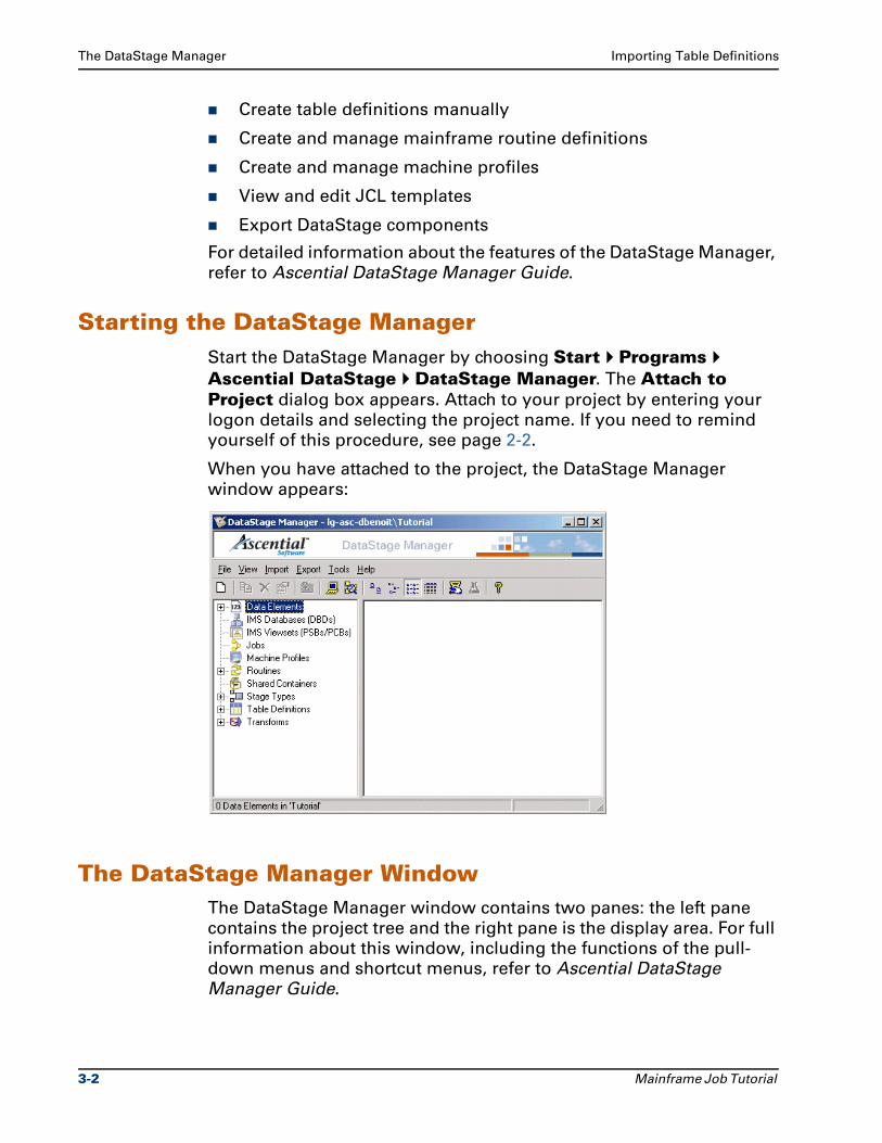
When you have attached to the project, the DataStage Manager
window appears:
The DataStage Manager WindowThe DataStage Manager window contains two panes: the left pane
contains the project tree and the right pane is the display area. For full
information about this window, including the functions of the pull-
down menus and shortcut menus, refer to Ascential DataStage
Manager Guide.
3-2 Mainframe Job Tutorial
Importing Table Definitions The DataStage Manager
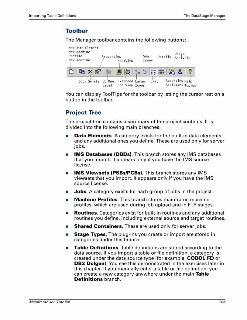
Toolbar
The Manager toolbar contains the following buttons:
You can display ToolTips for the toolbar by letting the cursor rest on a
button in the toolbar.
Project Tree
The project tree contains a summary of the project contents. It is
divided into the following main branches:
Data Elements. A category exists for the built-in data elements and any additional ones you define. These are used only for server jobs.
IMS Databases (DBDs). This branch stores any IMS databases that you import. It appears only if you have the IMS source license.
IMS Viewsets (PSBs/PCBs). This branch stores any IMS viewsets that you import. It appears only if you have the IMS source license.
Jobs. A category exists for each group of jobs in the project.
Machine Profiles. This branch stores mainframe machine profiles, which are used during job upload and in FTP stages.
Routines. Categories exist for built-in routines and any additional routines you define, including external source and target routines.
Shared Containers. These are used only for server jobs.
Stage Types. The plug-ins you create or import are stored in categories under this branch.
Table Definitions. Table definitions are stored according to the data source. If you import a table or file definition, a category is created under the data source type (for example, COBOL FD or DB2 Dclgen). You see this demonstrated in the exercises later in this chapter. If you manually enter a table or file definition, you can create a new category anywhere under the main Table Definitions branch.
New Data Element New Machine ProfileNew Routine
Copy Delete
Properties
Large Icons
Small Icons
List
Details
Reporting Assistant
Usage Analysis
Help Topics
Up One Level
HostView
Extended Job View
Mainframe Job Tutorial 3-3
Exercise 2: Import Mainframe Table Definitions Importing Table Definitions
Transforms. These apply only to server jobs. A category exists for the built-in transforms and for each group of custom transforms created.
Note If you select Host View from the toolbar, you will see all
projects on the server rather than just the categories for the
currently attached project. If you select Extended Job View you can view all the components and other ancillary
information contained within a job. For further details see
Ascential DataStage Manager Guide.
Display Area
The display area in the right pane of the Manager window is known as
the Project View. It displays the contents of the branch chosen in the
project tree. You can display items in the display area in one of four
ways:
Large icons. Items are displayed as large icons arranged across the display area.
Small icons. Items are displayed as small icons arranged across the display area.
List. Items are displayed in a list going down the display area.
Details. Items are displayed in a table with Name, Description, and Date/Time Modified columns.
Exercise 2: Import Mainframe Table DefinitionsIn this exercise you import table definitions (meta data) into the
Repository from the sample CFD and DCLGen files. These files are
located on the tutorial CD. Insert the CD into your CD-ROM drive
before you begin.
Importing CFD FilesFirst you import the table definitions in the ProductsCustomers.cfd and Salesord.cfd files. Each CFD file can contain more than one table
definition. In later chapters, you will practice what you learn here by
importing other CFDs.
3-4 Mainframe Job Tutorial
Importing Table Definitions Exercise 2: Import Mainframe Table Definitions
To import the CFD files:
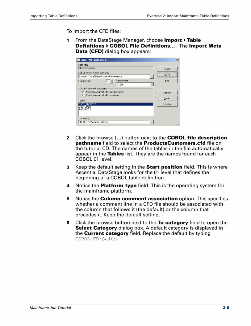
1 From the DataStage Manager, choose Import Table Definitions COBOL File Definitions… . The Import Meta Data (CFD) dialog box appears:
2 Click the browse (…) button next to the COBOL file description pathname field to select the ProductsCustomers.cfd file on the tutorial CD. The names of the tables in the file automatically appear in the Tables list. They are the names found for each COBOL 01 level.
3 Keep the default setting in the Start position field. This is where Ascential DataStage looks for the 01 level that defines the beginning of a COBOL table definition.
4 Notice the Platform type field. This is the operating system for the mainframe platform.
5 Notice the Column comment association option. This specifies whether a comment line in a CFD file should be associated with the column that follows it (the default) or the column that precedes it. Keep the default setting.
6 Click the browse button next to the To category field to open the Select Category dialog box. A default category is displayed in the Current category field. Replace the default by typing COBOL FD\Sales.
Mainframe Job Tutorial 3-5
Exercise 2: Import Mainframe Table Definitions Importing Table Definitions
Click OK to return to the Import Meta Data (CFD) dialog box.
7 Click Select all to select all of the files displayed in the Tables list, then click Import. Ascential DataStage imports the meta data and automatically creates table definitions in the Repository.
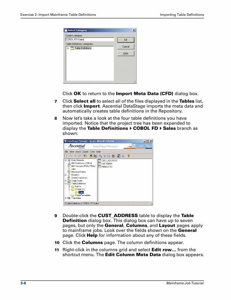
8 Now let’s take a look at the four table definitions you have imported. Notice that the project tree has been expanded to display the Table Definitions COBOL FD Sales branch as shown:
9 Double-click the CUST_ADDRESS table to display the Table Definition dialog box. This dialog box can have up to seven pages, but only the General, Columns, and Layout pages apply to mainframe jobs. Look over the fields shown on the General page. Click Help for information about any of these fields.
10 Click the Columns page. The column definitions appear.
11 Right-click in the columns grid and select Edit row… from the shortcut menu. The Edit Column Meta Data dialog box appears.
3-6 Mainframe Job Tutorial
Importing Table Definitions Exercise 2: Import Mainframe Table Definitions
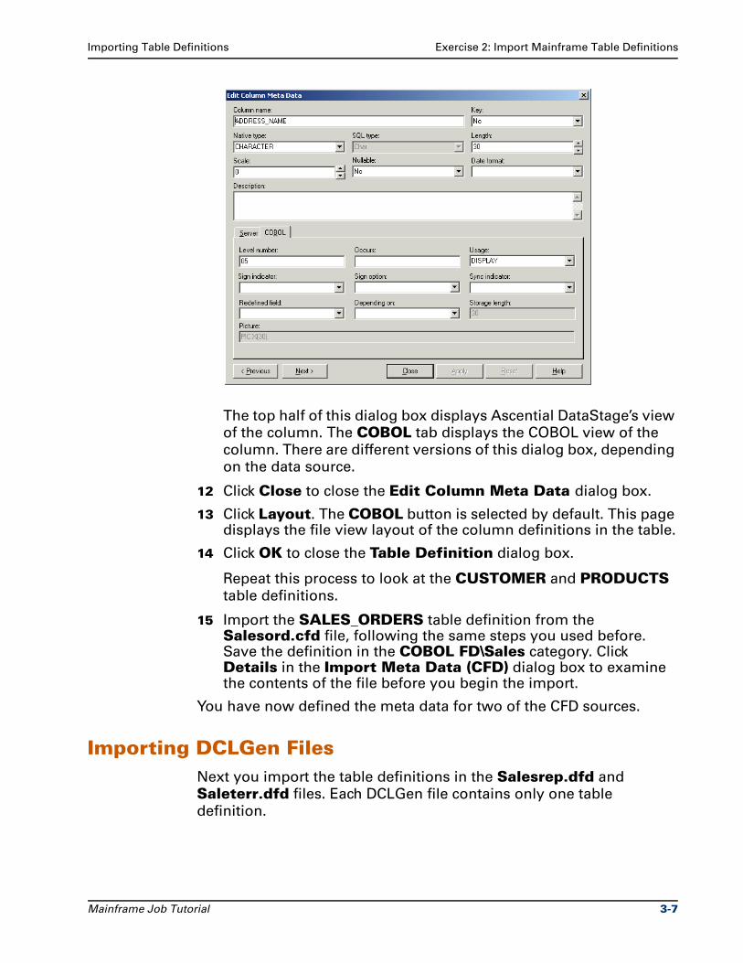
The top half of this dialog box displays Ascential DataStage’s view
of the column. The COBOL tab displays the COBOL view of the
column. There are different versions of this dialog box, depending
on the data source.
12 Click Close to close the Edit Column Meta Data dialog box.
13 Click Layout. The COBOL button is selected by default. This page displays the file view layout of the column definitions in the table.
14 Click OK to close the Table Definition dialog box.
Repeat this process to look at the CUSTOMER and PRODUCTS
table definitions.
15 Import the SALES_ORDERS table definition from the Salesord.cfd file, following the same steps you used before. Save the definition in the COBOL FD\Sales category. Click Details in the Import Meta Data (CFD) dialog box to examine the contents of the file before you begin the import.
You have now defined the meta data for two of the CFD sources.
Importing DCLGen FilesNext you import the table definitions in the Salesrep.dfd and
Saleterr.dfd files. Each DCLGen file contains only one table
definition.
Mainframe Job Tutorial 3-7
Summary Importing Table Definitions
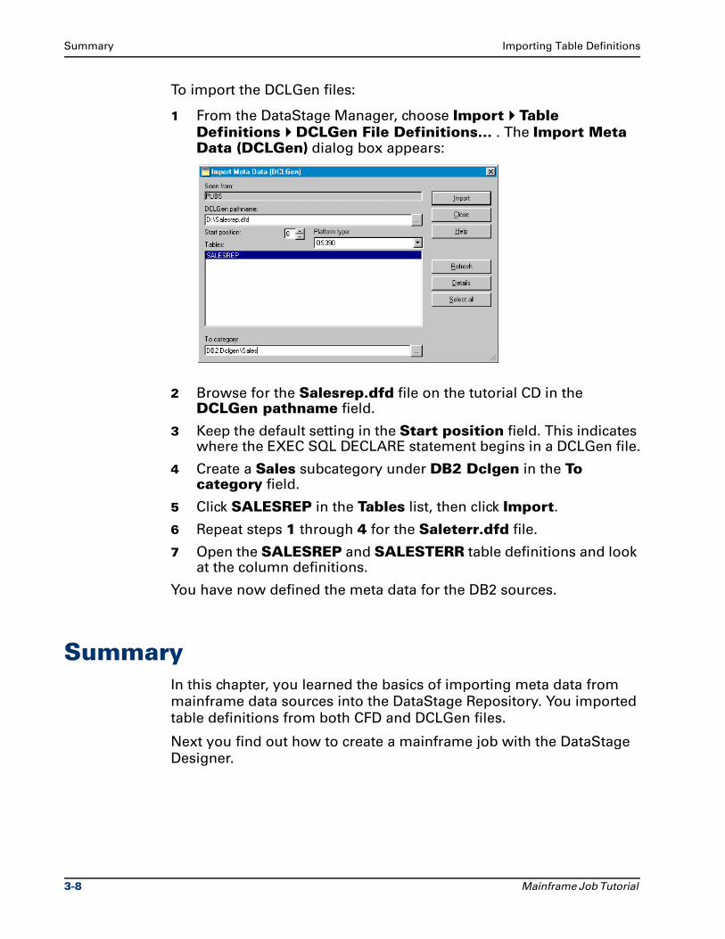
To import the DCLGen files:
1 From the DataStage Manager, choose Import Table Definitions DCLGen File Definitions… . The Import Meta Data (DCLGen) dialog box appears:
2 Browse for the Salesrep.dfd file on the tutorial CD in the DCLGen pathname field.
3 Keep the default setting in the Start position field. This indicates where the EXEC SQL DECLARE statement begins in a DCLGen file.
4 Create a Sales subcategory under DB2 Dclgen in the To category field.
5 Click SALESREP in the Tables list, then click Import.
6 Repeat steps 1 through 4 for the Saleterr.dfd file.
7 Open the SALESREP and SALESTERR table definitions and look at the column definitions.
You have now defined the meta data for the DB2 sources.
SummaryIn this chapter, you learned the basics of importing meta data from
mainframe data sources into the DataStage Repository. You imported
table definitions from both CFD and DCLGen files.
Next you find out how to create a mainframe job with the DataStage
Designer.
3-8 Mainframe Job Tutorial
4Designing a Mainframe Job
This chapter introduces you to designing mainframe jobs in the
DataStage Designer. You create a simple job that extracts data from a
flat file, transforms it, and loads it to a flat file. The focus is on
familiarizing you with the features of the Designer rather than
demonstrating the capabilities of the individual stage editors. You’ll
learn more about the mainframe stage editors in later chapters.
In Exercise 3 you learn how to specify Designer options for mainframe
jobs. Then in Exercise 4 you create a job consisting of the following
stages:
A Fixed-Width Flat File source stage to handle the extraction of data from the source file
A Transformer stage to link the input and output columns
A Fixed-Width Flat File target stage to handle the writing of data to the target file
As you design the job, you look at each stage to see how it is
configured. You see how easy it is to build the structure of a job in the
Designer and then bind specific files to that job. Finally, you generate
code for the job.
This is a very basic job, but it offers a good introduction to Ascential
DataStage. Using what you learn in this chapter, you will create more
advanced jobs later in the tutorial.
The DataStage DesignerThe DataStage Designer is where you build jobs using a visual design
that models the flow and transformation of data from the data sources
Mainframe Job Tutorial 4-1
The DataStage Designer Designing a Mainframe Job
through to the target data warehouse. The Designer’s graphical
interface lets you select stage icons, drop them onto the Designer
canvas, and add links. You then define the required actions and
processes for each stage and link using the individual stage editors.
Finally, you generate code.
Before you begin most of the exercises, you need to run the
DataStage Designer and become acquainted with the Designer
window. The tutorial describes the main features and tells you
enough about the Designer to enable you to complete the exercises.
For detailed information, refer to Ascential DataStage Designer Guide.
Starting the DataStage DesignerYou can move between the DataStage Manager and Designer using
the Tools menu. If you still have the Manager open from the last
exercise, start the Designer by choosing Tools Run Designer. You
are still attached to the same project.
If you closed the Manager, choose Start Programs Ascential DataStage DataStage Designer to run the Designer. The Attach to Project dialog box appears. Attach to your project by entering
your logon details.
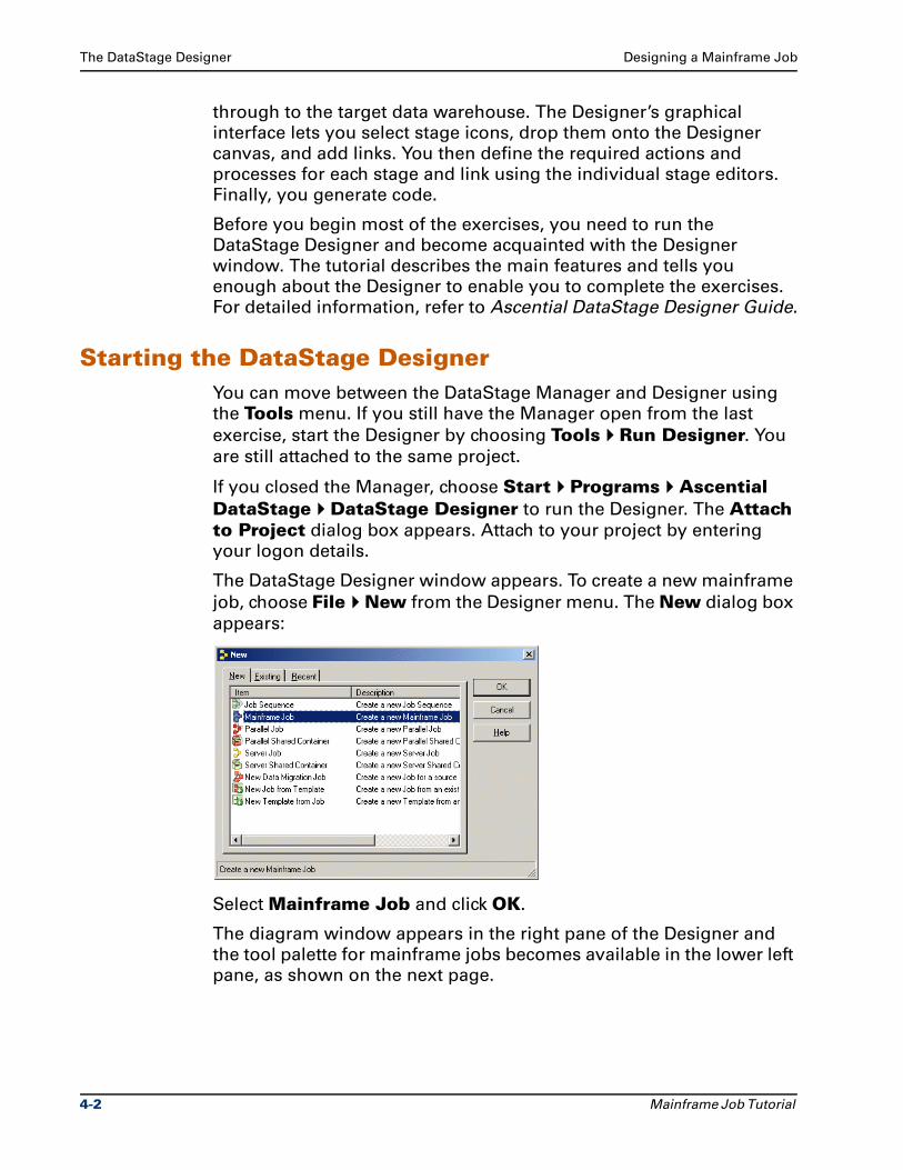
The DataStage Designer window appears. To create a new mainframe
job, choose File New from the Designer menu. The New dialog box
appears:
Select Mainframe Job and click OK.
The diagram window appears in the right pane of the Designer and
the tool palette for mainframe jobs becomes available in the lower left
pane, as shown on the next page.
4-2 Mainframe Job Tutorial
Designing a Mainframe Job The DataStage Designer
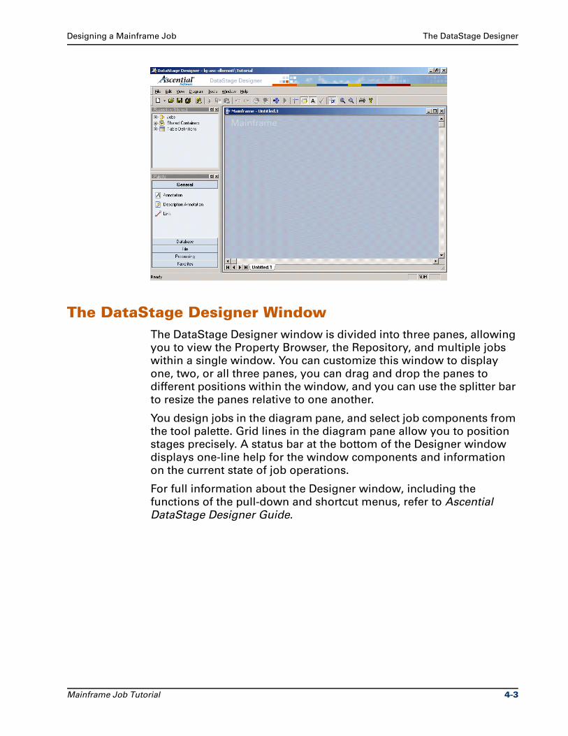
The DataStage Designer WindowThe DataStage Designer window is divided into three panes, allowing
you to view the Property Browser, the Repository, and multiple jobs
within a single window. You can customize this window to display
one, two, or all three panes, you can drag and drop the panes to
different positions within the window, and you can use the splitter bar
to resize the panes relative to one another.
You design jobs in the diagram pane, and select job components from
the tool palette. Grid lines in the diagram pane allow you to position
stages precisely. A status bar at the bottom of the Designer window
displays one-line help for the window components and information
on the current state of job operations.
For full information about the Designer window, including the
functions of the pull-down and shortcut menus, refer to Ascential
DataStage Designer Guide.
Mainframe Job Tutorial 4-3
The DataStage Designer Designing a Mainframe Job
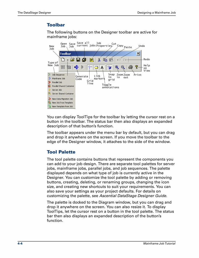
Toolbar
The following buttons on the Designer toolbar are active for
mainframe jobs:
You can display ToolTips for the toolbar by letting the cursor rest on a
button in the toolbar. The status bar then also displays an expanded
description of that button’s function.
The toolbar appears under the menu bar by default, but you can drag
and drop it anywhere on the screen. If you move the toolbar to the
edge of the Designer window, it attaches to the side of the window.
Tool Palette
The tool palette contains buttons that represent the components you
can add to your job design. There are separate tool palettes for server
jobs, mainframe jobs, parallel jobs, and job sequences. The palette
displayed depends on what type of job is currently active in the
Designer. You can customize the tool palette by adding or removing
buttons, creating, deleting, or renaming groups, changing the icon
size, and creating new shortcuts to suit your requirements. You can
also save your settings as your project defaults. For details on
customizing the palette, see Ascential DataStage Designer Guide.
The palette is docked to the Diagram window, but you can drag and
drop it anywhere on the screen. You can also resize it. To display
ToolTips, let the cursor rest on a button in the tool palette. The status
bar then also displays an expanded description of the button’s
function.
Snap to grid
Help onView
Save JobNew
Job
Generate Code
Grid line Toggle
annotations
PrintZoom out
Zoom in
Open Job
Type of New Job
Save all current jobs
Link markers
CutCopy
Paste Undo
Redo
Job Properties
4-4 Mainframe Job Tutorial
Designing a Mainframe Job The DataStage Designer
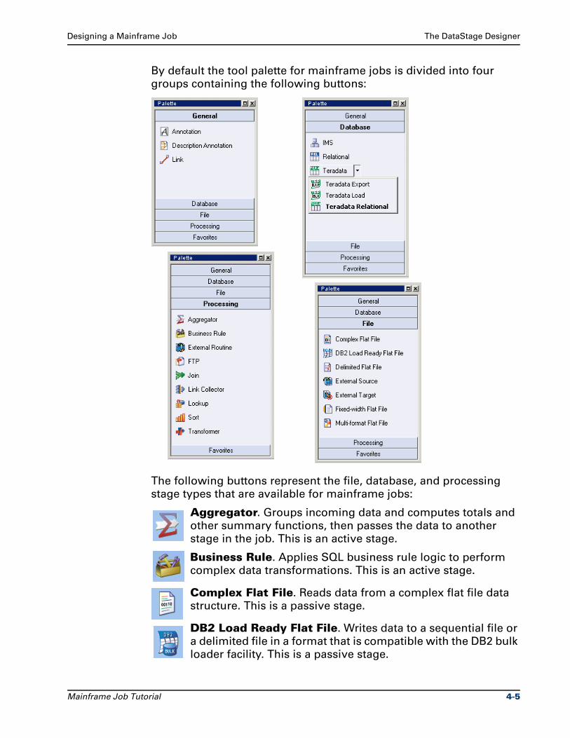
By default the tool palette for mainframe jobs is divided into four
groups containing the following buttons:
The following buttons represent the file, database, and processing
stage types that are available for mainframe jobs:
Aggregator. Groups incoming data and computes totals and
other summary functions, then passes the data to another
stage in the job. This is an active stage.
Business Rule. Applies SQL business rule logic to perform
complex data transformations. This is an active stage.
Complex Flat File. Reads data from a complex flat file data
structure. This is a passive stage.
DB2 Load Ready Flat File. Writes data to a sequential file or
a delimited file in a format that is compatible with the DB2 bulk
loader facility. This is a passive stage.
Mainframe Job Tutorial 4-5
The DataStage Designer Designing a Mainframe Job
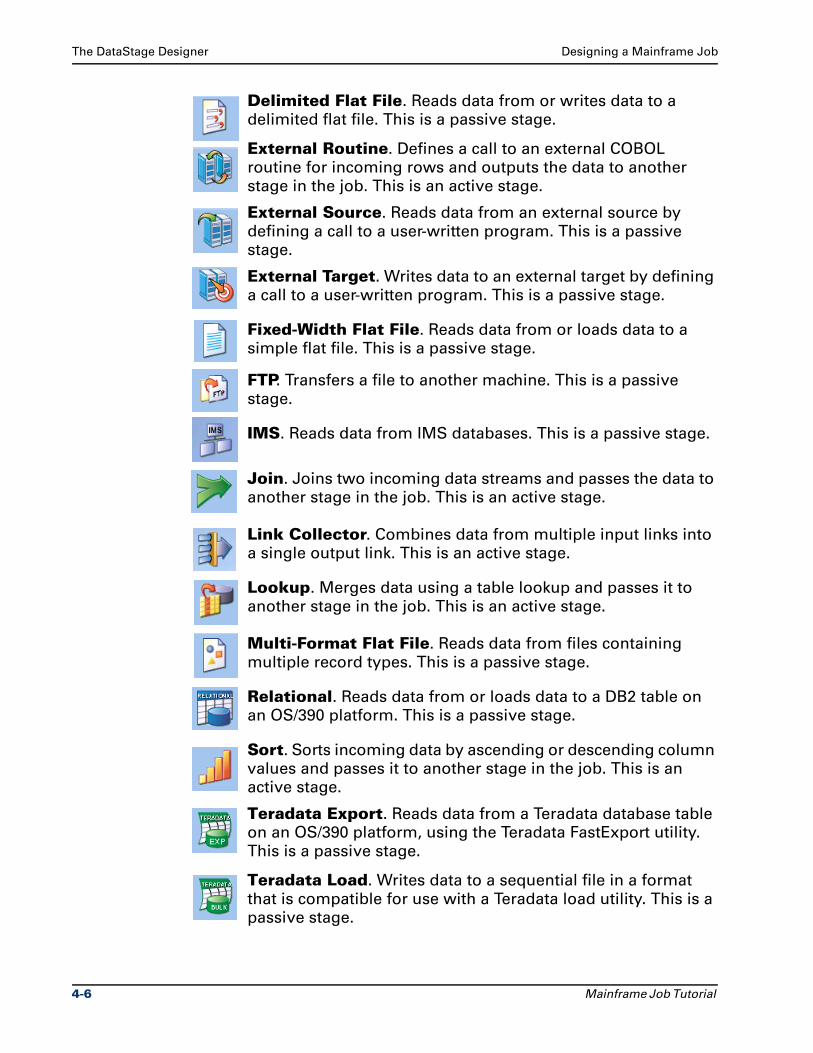
Delimited Flat File. Reads data from or writes data to a
delimited flat file. This is a passive stage.
External Routine. Defines a call to an external COBOL
routine for incoming rows and outputs the data to another
stage in the job. This is an active stage.
External Source. Reads data from an external source by
defining a call to a user-written program. This is a passive
stage.
External Target. Writes data to an external target by defining
a call to a user-written program. This is a passive stage.
Fixed-Width Flat File. Reads data from or loads data to a
simple flat file. This is a passive stage.
FTP. Transfers a file to another machine. This is a passive
stage.
IMS. Reads data from IMS databases. This is a passive stage.
Join. Joins two incoming data streams and passes the data to
another stage in the job. This is an active stage.
Link Collector. Combines data from multiple input links into
a single output link. This is an active stage.
Lookup. Merges data using a table lookup and passes it to
another stage in the job. This is an active stage.
Multi-Format Flat File. Reads data from files containing
multiple record types. This is a passive stage.
Relational. Reads data from or loads data to a DB2 table on
an OS/390 platform. This is a passive stage.
Sort. Sorts incoming data by ascending or descending column
values and passes it to another stage in the job. This is an
active stage.
Teradata Export. Reads data from a Teradata database table
on an OS/390 platform, using the Teradata FastExport utility.
This is a passive stage.
Teradata Load. Writes data to a sequential file in a format
that is compatible for use with a Teradata load utility. This is a
passive stage.
4-6 Mainframe Job Tutorial
Designing a Mainframe Job Exercise 3: Specify Designer Options
Teradata Relational. Reads data from or writes data to a
Teradata database table on an OS/390 platform. This is a
passive stage.
Transformer. Filters and transforms incoming data, then
outputs it to another stage in the job. This is an active stage.
The General group on the tool palette contains three additional icons:
Annotation. Contains notes that you enter to describe the
stages or links in a job.
Description Annotation. Displays either the short or long
description from the job properties. You can edit this within
the annotation if required. There is only one of these per job.
Link. Joins the stages in a job together.
Exercise 3: Specify Designer OptionsBefore you design a job, you specify Designer default options that
apply to all mainframe jobs. For information about setting other
Designer defaults, see Ascential DataStage Designer Guide.
To set Designer defaults for mainframe jobs:
1 Choose Tools Options from the Designer menu. The Options dialog box appears. This dialog box has a tree in the left pane with eight branches, each containing settings for individual areas of the Designer.
2 Select the Default branch to specify how the Designer should behave when started. In the When Designer starts area, click Create new and select Mainframe from the drop-down list. From now on, a new, empty mainframe job will automatically be created whenever you start the Designer.
Mainframe Job Tutorial 4-7
Exercise 3: Specify Designer Options Designing a Mainframe Job
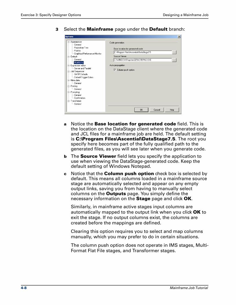
3 Select the Mainframe page under the Default branch:
a Notice the Base location for generated code field. This is the location on the DataStage client where the generated code and JCL files for a mainframe job are held. The default setting is C:\Program Files\Ascential\DataStage7.5. The root you specify here becomes part of the fully qualified path to the generated files, as you will see later when you generate code.
b The Source Viewer field lets you specify the application to use when viewing the DataStage-generated code. Keep the default setting of Windows Notepad.
c Notice that the Column push option check box is selected by default. This means all columns loaded in a mainframe source stage are automatically selected and appear on any empty output links, saving you from having to manually select columns on the Outputs page. You simply define the necessary information on the Stage page and click OK.
Similarly, in mainframe active stages input columns are
automatically mapped to the output link when you click OK to
exit the stage. If no output columns exist, the columns are
created before the mappings are defined.
Clearing this option requires you to select and map columns
manually, which you may prefer to do in certain situations.
The column push option does not operate in IMS stages, Multi-
Format Flat File stages, and Transformer stages.
4-8 Mainframe Job Tutorial
Designing a Mainframe Job Exercise 4: Create a Mainframe Job
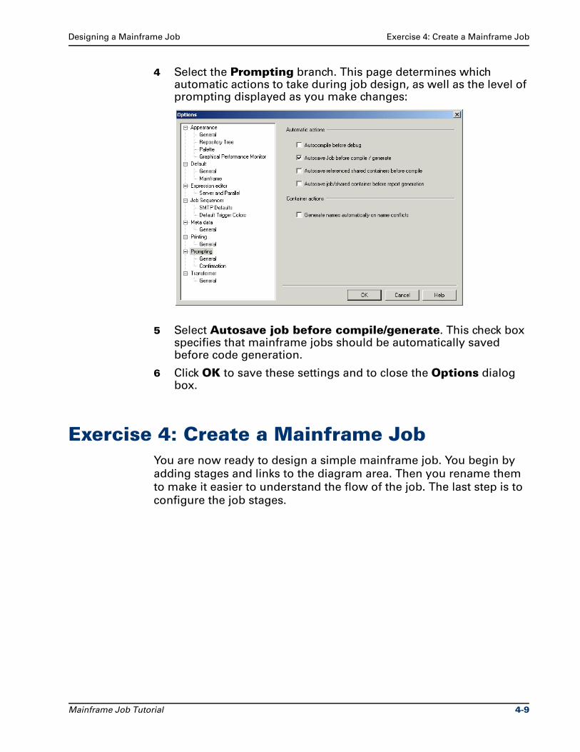
4 Select the Prompting branch. This page determines which automatic actions to take during job design, as well as the level of prompting displayed as you make changes:
5 Select Autosave job before compile/generate. This check box specifies that mainframe jobs should be automatically saved before code generation.
6 Click OK to save these settings and to close the Options dialog box.
Exercise 4: Create a Mainframe JobYou are now ready to design a simple mainframe job. You begin by
adding stages and links to the diagram area. Then you rename them
to make it easier to understand the flow of the job. The last step is to
configure the job stages.
Mainframe Job Tutorial 4-9
Exercise 4: Create a Mainframe Job Designing a Mainframe Job
Designing the JobTo design your mainframe job in the DataStage Designer:
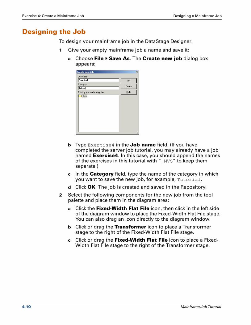
1 Give your empty mainframe job a name and save it:
a Choose File Save As. The Create new job dialog box appears:
b Type Exercise4 in the Job name field. (If you have completed the server job tutorial, you may already have a job named Exercise4. In this case, you should append the names of the exercises in this tutorial with “_MVS” to keep them separate.)
c In the Category field, type the name of the category in which you want to save the new job, for example, Tutorial.
d Click OK. The job is created and saved in the Repository.
2 Select the following components for the new job from the tool palette and place them in the diagram area:
a Click the Fixed-Width Flat File icon, then click in the left side of the diagram window to place the Fixed-Width Flat File stage. You can also drag an icon directly to the diagram window.
b Click or drag the Transformer icon to place a Transformer stage to the right of the Fixed-Width Flat File stage.
c Click or drag the Fixed-Width Flat File icon to place a Fixed-Width Flat File stage to the right of the Transformer stage.
4-10 Mainframe Job Tutorial
Designing a Mainframe Job Exercise 4: Create a Mainframe Job
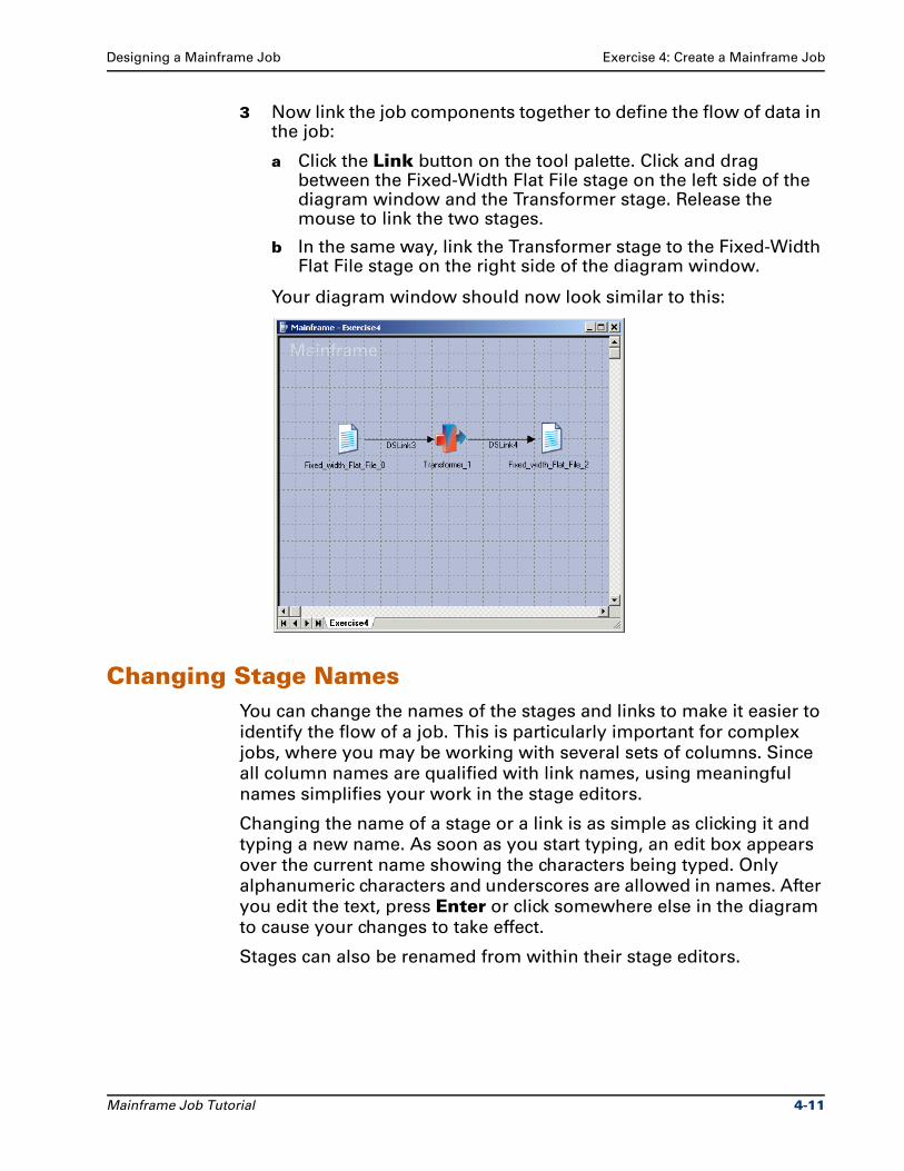
3 Now link the job components together to define the flow of data in the job:
a Click the Link button on the tool palette. Click and drag between the Fixed-Width Flat File stage on the left side of the diagram window and the Transformer stage. Release the mouse to link the two stages.
b In the same way, link the Transformer stage to the Fixed-Width Flat File stage on the right side of the diagram window.
Your diagram window should now look similar to this:
Changing Stage NamesYou can change the names of the stages and links to make it easier to
identify the flow of a job. This is particularly important for complex
jobs, where you may be working with several sets of columns. Since
all column names are qualified with link names, using meaningful
names simplifies your work in the stage editors.
Changing the name of a stage or a link is as simple as clicking it and
typing a new name. As soon as you start typing, an edit box appears
over the current name showing the characters being typed. Only
alphanumeric characters and underscores are allowed in names. After
you edit the text, press Enter or click somewhere else in the diagram
to cause your changes to take effect.
Stages can also be renamed from within their stage editors.
Mainframe Job Tutorial 4-11
Exercise 4: Create a Mainframe Job Designing a Mainframe Job
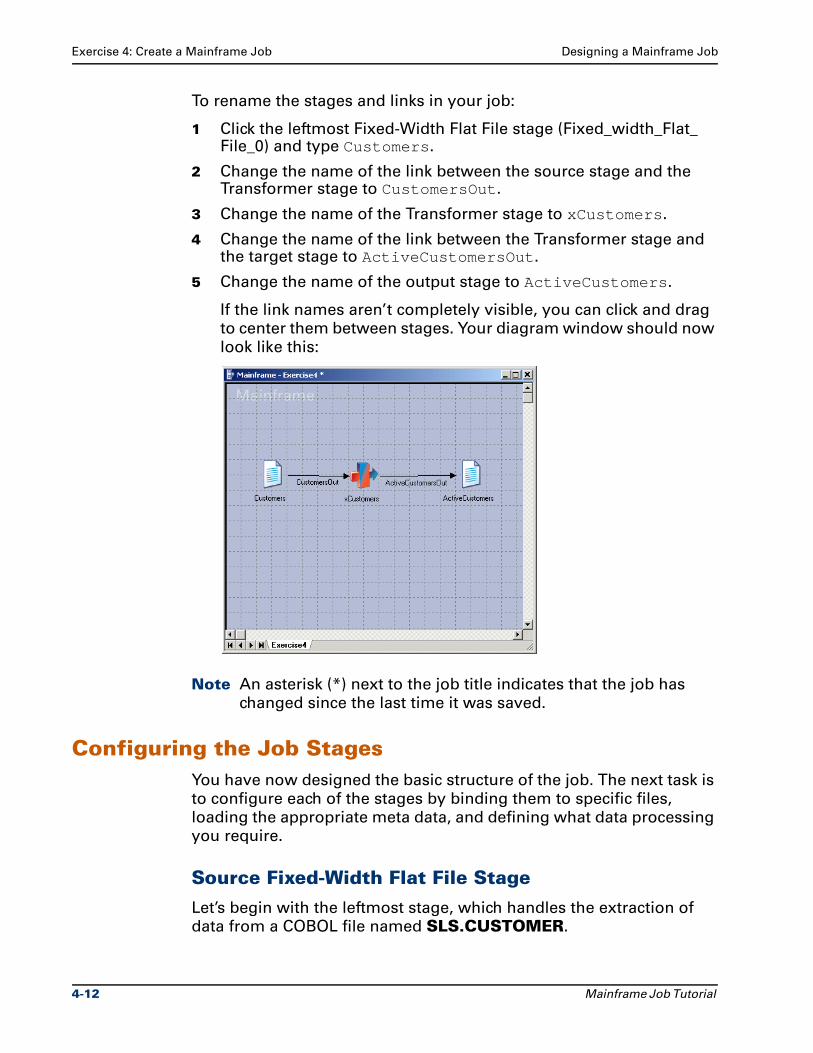
To rename the stages and links in your job:
1 Click the leftmost Fixed-Width Flat File stage (Fixed_width_Flat_File_0) and type Customers.
2 Change the name of the link between the source stage and the Transformer stage to CustomersOut.
3 Change the name of the Transformer stage to xCustomers.
4 Change the name of the link between the Transformer stage and the target stage to ActiveCustomersOut.
5 Change the name of the output stage to ActiveCustomers.
If the link names aren’t completely visible, you can click and drag
to center them between stages. Your diagram window should now
look like this:
Note An asterisk (*) next to the job title indicates that the job has
changed since the last time it was saved.
Configuring the Job StagesYou have now designed the basic structure of the job. The next task is
to configure each of the stages by binding them to specific files,
loading the appropriate meta data, and defining what data processing
you require.
Source Fixed-Width Flat File Stage
Let’s begin with the leftmost stage, which handles the extraction of
data from a COBOL file named SLS.CUSTOMER.
4-12 Mainframe Job Tutorial
Designing a Mainframe Job Exercise 4: Create a Mainframe Job
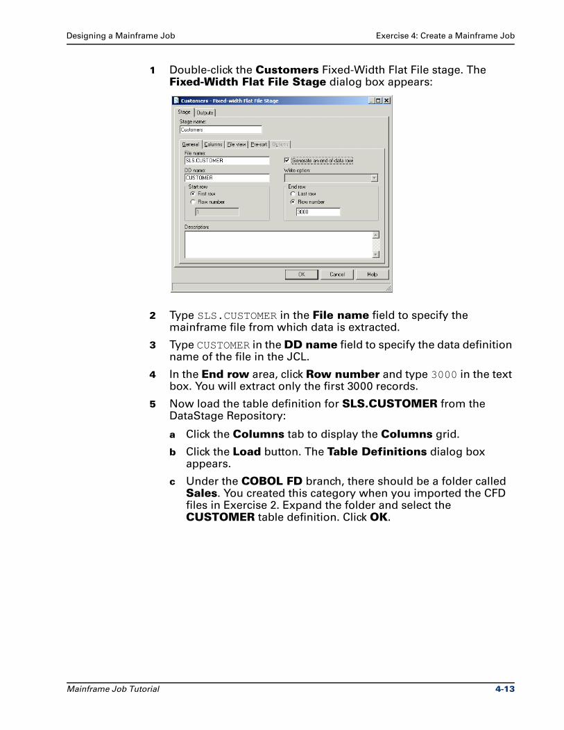
1 Double-click the Customers Fixed-Width Flat File stage. The Fixed-Width Flat File Stage dialog box appears:
2 Type SLS.CUSTOMER in the File name field to specify the mainframe file from which data is extracted.
3 Type CUSTOMER in the DD name field to specify the data definition name of the file in the JCL.
4 In the End row area, click Row number and type 3000 in the text box. You will extract only the first 3000 records.
5 Now load the table definition for SLS.CUSTOMER from the DataStage Repository:
a Click the Columns tab to display the Columns grid.
b Click the Load button. The Table Definitions dialog box appears.
c Under the COBOL FD branch, there should be a folder called Sales. You created this category when you imported the CFD files in Exercise 2. Expand the folder and select the CUSTOMER table definition. Click OK.
Mainframe Job Tutorial 4-13
Exercise 4: Create a Mainframe Job Designing a Mainframe Job
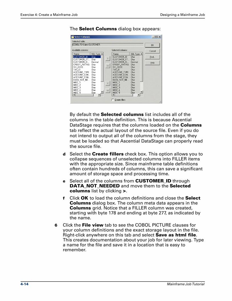
The Select Columns dialog box appears:
By default the Selected columns list includes all of the
columns in the table definition. This is because Ascential
DataStage requires that the columns loaded on the Columns
tab reflect the actual layout of the source file. Even if you do
not intend to output all of the columns from the stage, they
must be loaded so that Ascential DataStage can properly read
the source file.
d Select the Create fillers check box. This option allows you to collapse sequences of unselected columns into FILLER items with the appropriate size. Since mainframe table definitions often contain hundreds of columns, this can save a significant amount of storage space and processing time.
e Select all of the columns from CUSTOMER_ID through DATA_NOT_NEEDED and move them to the Selected columns list by clicking >.
f Click OK to load the column definitions and close the Select Columns dialog box. The column meta data appears in the Columns grid. Notice that a FILLER column was created, starting with byte 178 and ending at byte 277, as indicated by the name.
6 Click the File view tab to see the COBOL PICTURE clauses for your column definitions and the exact storage layout in the file. Right-click anywhere on this tab and select Save as html file. This creates documentation about your job for later viewing. Type a name for the file and save it in a location that is easy to remember.
4-14 Mainframe Job Tutorial
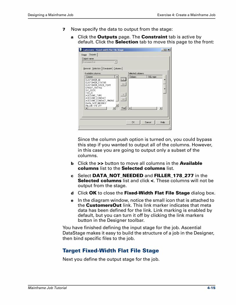
Designing a Mainframe Job Exercise 4: Create a Mainframe Job
7 Now specify the data to output from the stage:
a Click the Outputs page. The Constraint tab is active by default. Click the Selection tab to move this page to the front:
Since the column push option is turned on, you could bypass
this step if you wanted to output all of the columns. However,
in this case you are going to output only a subset of the
columns.
b Click the >> button to move all columns in the Available columns list to the Selected columns list.
c Select DATA_NOT_NEEDED and FILLER_178_277 in the Selected columns list and click <. These columns will not be output from the stage.
d Click OK to close the Fixed-Width Flat File Stage dialog box.
e In the diagram window, notice the small icon that is attached to the CustomersOut link. This link marker indicates that meta data has been defined for the link. Link marking is enabled by default, but you can turn it off by clicking the link markers button in the Designer toolbar.
You have finished defining the input stage for the job. Ascential
DataStage makes it easy to build the structure of a job in the Designer,
then bind specific files to the job.
Target Fixed-Width Flat File Stage
Next you define the output stage for the job.
Mainframe Job Tutorial 4-15
Exercise 4: Create a Mainframe Job Designing a Mainframe Job
1 Double-click the ActiveCustomers Fixed-Width Flat File stage. The Fixed-Width Flat File Stage dialog box appears. Notice that the dialog box for this stage does not show an Outputs page, but an Inputs page instead. Since this is the last stage in the job, it has no outputs to other stages. It only accepts input from the previous stage.
2 Specify the name of the target file and the write option:
a Type SLS.ACTCUST in the File name field.
b Type ACTCUST in the DD name field.
c Select Overwrite existing file from the Write option drop-down list. This indicates that SLS.ACTCUST is an existing file and you will overwrite any existing data in the file.
3 As you did for the input stage, you define the data in ActiveCustomers by loading a table definition from the Repository. Since you are going to perform simple mappings in the Transformer stage without changing field formats, you can load the same column definitions as were used in the input stage:
a Click the Columns tab.
b Click Load, then select CUSTOMER from the COBOL FD\ Sales branch in the Table Definitions dialog box, and click OK.
c Remove the columns DATA_NOT_NEEDED through MISC_10 from the Selected columns list in the Select Columns dialog box, then click OK.
4 Click OK to close the Fixed-Width Flat File Stage dialog box. You have finished creating the output stage for the job. A link marker appears in the diagram window, showing that meta data has been defined for the ActiveCustomersOut link.
Transformer Stage
With the input and output stages of the job defined, the next step is to
define the Transformer stage. This is the stage where you specify
what transformations you want to apply to the data before it is output
to the target file.
4-16 Mainframe Job Tutorial
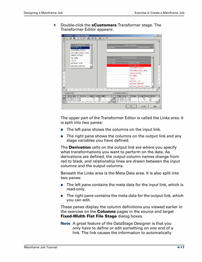
Designing a Mainframe Job Exercise 4: Create a Mainframe Job
1 Double-click the xCustomers Transformer stage. The Transformer Editor appears:
The upper part of the Transformer Editor is called the Links area. It
is split into two panes:
The left pane shows the columns on the input link.
The right pane shows the columns on the output link and any stage variables you have defined.
The Derivation cells on the output link are where you specify
what transformations you want to perform on the data. As
derivations are defined, the output column names change from
red to black, and relationship lines are drawn between the input
columns and the output columns.
Beneath the Links area is the Meta Data area. It is also split into
two panes:
The left pane contains the meta data for the input link, which is read-only.
The right pane contains the meta data for the output link, which you can edit.
These panes display the column definitions you viewed earlier in
the exercise on the Columns pages in the source and target
Fixed-Width Flat File Stage dialog boxes.
Note A great feature of the DataStage Designer is that you
only have to define or edit something on one end of a
link. The link causes the information to automatically
Mainframe Job Tutorial 4-17
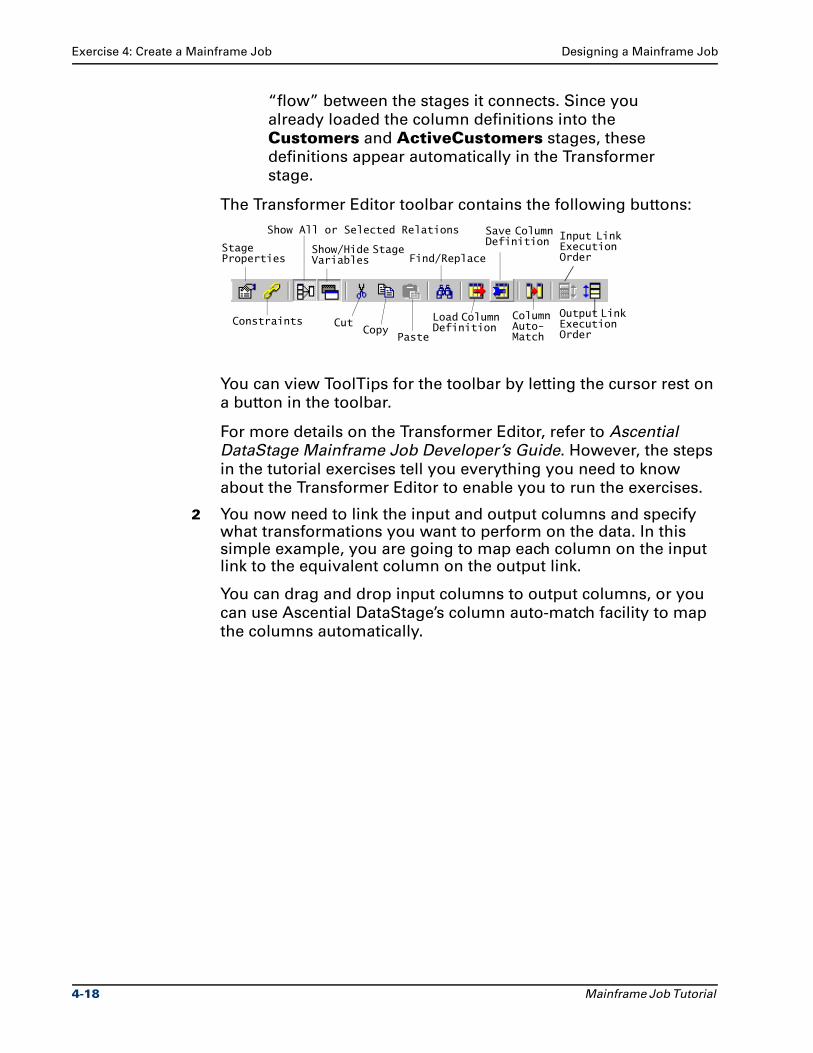
Exercise 4: Create a Mainframe Job Designing a Mainframe Job
“flow” between the stages it connects. Since you
already loaded the column definitions into the
Customers and ActiveCustomers stages, these
definitions appear automatically in the Transformer
stage.
The Transformer Editor toolbar contains the following buttons:
You can view ToolTips for the toolbar by letting the cursor rest on
a button in the toolbar.
For more details on the Transformer Editor, refer to Ascential
DataStage Mainframe Job Developer’s Guide. However, the steps
in the tutorial exercises tell you everything you need to know
about the Transformer Editor to enable you to run the exercises.
2 You now need to link the input and output columns and specify what transformations you want to perform on the data. In this simple example, you are going to map each column on the input link to the equivalent column on the output link.
You can drag and drop input columns to output columns, or you
can use Ascential DataStage’s column auto-match facility to map
the columns automatically.
Show/Hide Stage Variables
Stage Properties
Constraints
Show All or Selected Relations
CutCopy
Paste
Find/Replace
Load Column Definition
Column Auto-Match
Save Column Definition Input Link
Execution Order
Output Link ExecutionOrder
4-18 Mainframe Job Tutorial
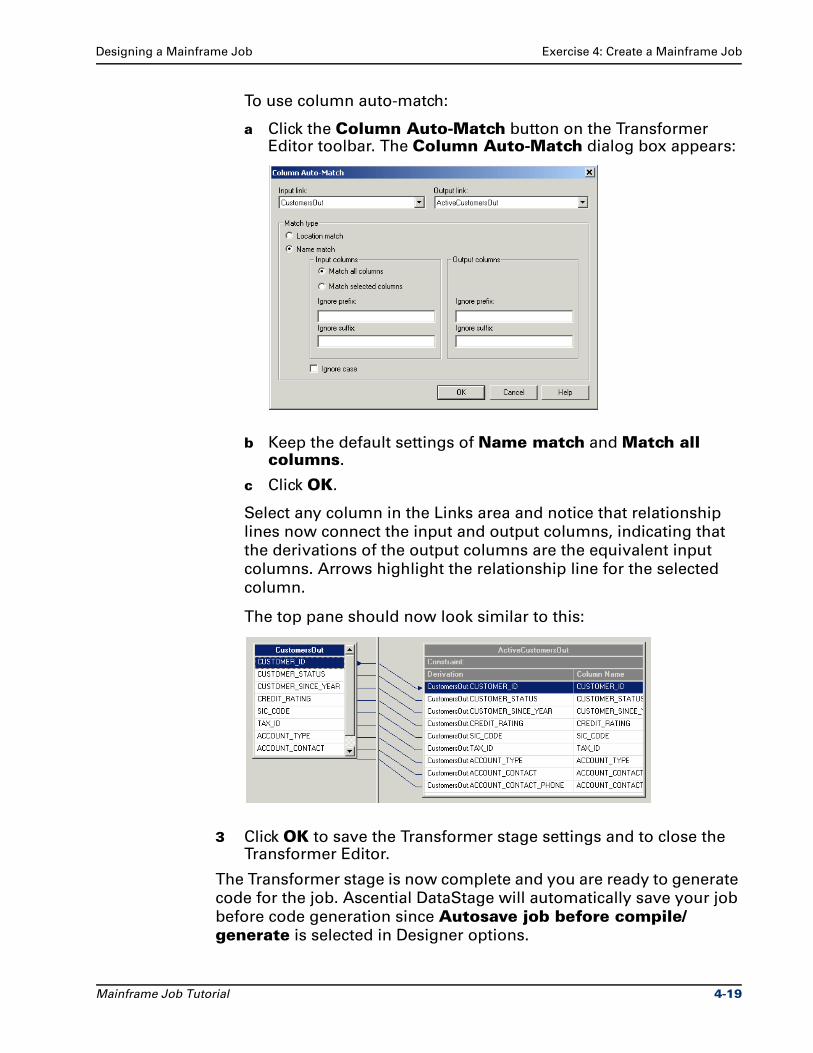
Designing a Mainframe Job Exercise 4: Create a Mainframe Job
To use column auto-match:
a Click the Column Auto-Match button on the Transformer Editor toolbar. The Column Auto-Match dialog box appears:
b Keep the default settings of Name match and Match all columns.
c Click OK.
Select any column in the Links area and notice that relationship
lines now connect the input and output columns, indicating that
the derivations of the output columns are the equivalent input
columns. Arrows highlight the relationship line for the selected
column.
The top pane should now look similar to this:
3 Click OK to save the Transformer stage settings and to close the Transformer Editor.
The Transformer stage is now complete and you are ready to generate
code for the job. Ascential DataStage will automatically save your job
before code generation since Autosave job before compile/generate is selected in Designer options.
Mainframe Job Tutorial 4-19
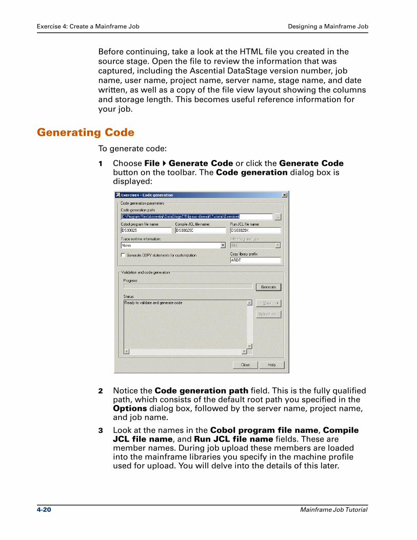
Exercise 4: Create a Mainframe Job Designing a Mainframe Job
Before continuing, take a look at the HTML file you created in the
source stage. Open the file to review the information that was
captured, including the Ascential DataStage version number, job
name, user name, project name, server name, stage name, and date
written, as well as a copy of the file view layout showing the columns
and storage length. This becomes useful reference information for
your job.
Generating CodeTo generate code:
1 Choose File Generate Code or click the Generate Code button on the toolbar. The Code generation dialog box is displayed:
2 Notice the Code generation path field. This is the fully qualified path, which consists of the default root path you specified in the Options dialog box, followed by the server name, project name, and job name.
3 Look at the names in the Cobol program file name, Compile JCL file name, and Run JCL file name fields. These are member names. During job upload these members are loaded into the mainframe libraries you specify in the machine profile used for upload. You will delve into the details of this later.
4-20 Mainframe Job Tutorial
Designing a Mainframe Job Summary
Note Once you generate code for a job, Ascential DataStage
remembers the information you specify in the Code generation parameters area. Even if you modify the
job and rename it, the original path and file names
appear in the Code generation dialog box. Be sure to
change these parameters if you do not want to
overwrite the previously generated files.
4 Click Generate to validate your job design and generate the COBOL program and JCL files. Progress is shown in the Progress bar and status messages appear in the Status window.
5 Click View to look at the generated files. When you are finished, click Close to close the Code generation dialog box.
This exercise has laid the foundation for more complex jobs in the
coming chapters. We have taken you through this exercise fairly
slowly to demonstrate the mechanics of designing a job and
configuring stages.
SummaryIn this chapter, you learned how to design a simple job. You created
source and target Fixed-Width Flat File stages and a Transformer
stage to link input columns to output columns. You used the
DataStage Designer to go through the process of building, saving, and
generating code for a job.
Next, you try some more advanced techniques. You use the
mainframe Expression Editor to build derivation expressions and
constraints. From this point forward, the exercises give shorter
directions for steps you have already performed. It is assumed that
you are now familiar with the Designer and Manager interfaces and
that you understand the basics of designing jobs and editing stages.
Detailed instructions are provided, however, for new tasks.
Mainframe Job Tutorial 4-21
5Defining Constraints and Derivations
This chapter shows you how to use the Expression Editor to define
constraints and column derivations in mainframe jobs. You also learn
how to specify job parameters and stage variables and incorporate
them into constraint and derivation expressions.
In Exercise 5 you define constraints to filter output data. You expand
the job you created in Exercise 4 by adding two more target stages.
You then use the constraints to conditionally direct data down the
different output links, including a reject link. You also define the link
execution order.
In Exercise 6 you specify a stage variable that derives customer
account descriptions. You insert a new column into each of your
output links, then use the stage variable in the output column
derivations. You then finish configuring the two target stages.
In Exercise 7 you define and use a job parameter related to customer
credit ratings. You modify the constraint created in Exercise 5 so that
only customers with a selected credit rating are written to the output
links.
Exercise 5: Define a ConstraintIn this exercise you learn how to define a constraint in a Transformer
stage. Using the Expression Editor, you select items and operators to
build the constraint expression. Constraints are boolean expressions
that return TRUE or FALSE.
Mainframe Job Tutorial 5-1
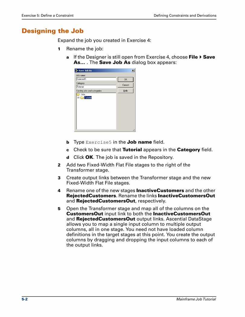
Exercise 5: Define a Constraint Defining Constraints and Derivations
Designing the JobExpand the job you created in Exercise 4:
1 Rename the job:
a If the Designer is still open from Exercise 4, choose File Save As… . The Save Job As dialog box appears:
b Type Exercise5 in the Job name field.
c Check to be sure that Tutorial appears in the Category field.
d Click OK. The job is saved in the Repository.
2 Add two Fixed-Width Flat File stages to the right of the Transformer stage.
3 Create output links between the Transformer stage and the new Fixed-Width Flat File stages.
4 Rename one of the new stages InactiveCustomers and the other RejectedCustomers. Rename the links InactiveCustomersOut and RejectedCustomersOut, respectively.
5 Open the Transformer stage and map all of the columns on the CustomersOut input link to both the InactiveCustomersOut and RejectedCustomersOut output links. Ascential DataStage allows you to map a single input column to multiple output columns, all in one stage. You need not have loaded column definitions in the target stages at this point. You create the output columns by dragging and dropping the input columns to each of the output links.
5-2 Mainframe Job Tutorial
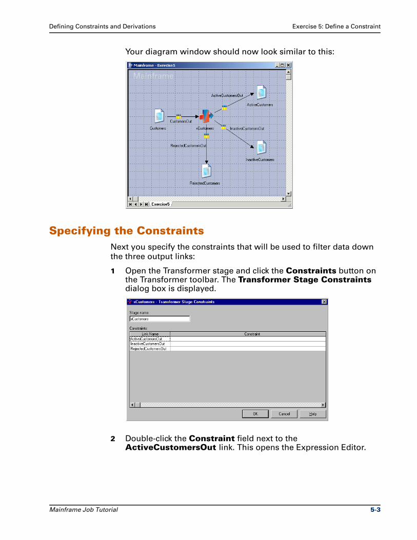
Defining Constraints and Derivations Exercise 5: Define a Constraint
Your diagram window should now look similar to this:
Specifying the ConstraintsNext you specify the constraints that will be used to filter data down
the three output links:
1 Open the Transformer stage and click the Constraints button on the Transformer toolbar. The Transformer Stage Constraints dialog box is displayed.
2 Double-click the Constraint field next to the ActiveCustomersOut link. This opens the Expression Editor.
Mainframe Job Tutorial 5-3
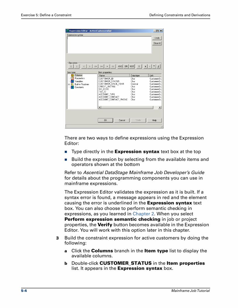
Exercise 5: Define a Constraint Defining Constraints and Derivations
There are two ways to define expressions using the Expression
Editor:
Type directly in the Expression syntax text box at the top
Build the expression by selecting from the available items and operators shown at the bottom
Refer to Ascential DataStage Mainframe Job Developer’s Guide
for details about the programming components you can use in
mainframe expressions.
The Expression Editor validates the expression as it is built. If a
syntax error is found, a message appears in red and the element
causing the error is underlined in the Expression syntax text
box. You can also choose to perform semantic checking in
expressions, as you learned in Chapter 2. When you select
Perform expression semantic checking in job or project
properties, the Verify button becomes available in the Expression
Editor. You will work with this option later in this chapter.
3 Build the constraint expression for active customers by doing the following:
a Click the Columns branch in the Item type list to display the available columns.
b Double-click CUSTOMER_STATUS in the Item properties list. It appears in the Expression syntax box.
5-4 Mainframe Job Tutorial
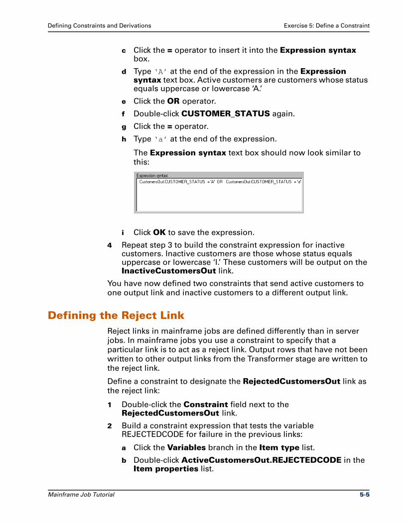
Defining Constraints and Derivations Exercise 5: Define a Constraint
c Click the = operator to insert it into the Expression syntax box.
d Type ‘A’ at the end of the expression in the Expression syntax text box. Active customers are customers whose status equals uppercase or lowercase ‘A.’
e Click the OR operator.
f Double-click CUSTOMER_STATUS again.
g Click the = operator.
h Type ‘a’ at the end of the expression.
The Expression syntax text box should now look similar to
this:
i Click OK to save the expression.
4 Repeat step 3 to build the constraint expression for inactive customers. Inactive customers are those whose status equals uppercase or lowercase ‘I.’ These customers will be output on the InactiveCustomersOut link.
You have now defined two constraints that send active customers to
one output link and inactive customers to a different output link.
Defining the Reject LinkReject links in mainframe jobs are defined differently than in server
jobs. In mainframe jobs you use a constraint to specify that a
particular link is to act as a reject link. Output rows that have not been
written to other output links from the Transformer stage are written to
the reject link.
Define a constraint to designate the RejectedCustomersOut link as
the reject link:
1 Double-click the Constraint field next to the RejectedCustomersOut link.
2 Build a constraint expression that tests the variable REJECTEDCODE for failure in the previous links:
a Click the Variables branch in the Item type list.
b Double-click ActiveCustomersOut.REJECTEDCODE in the Item properties list.
Mainframe Job Tutorial 5-5
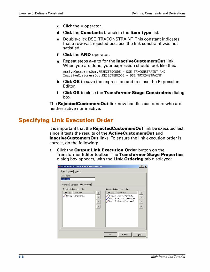
Exercise 5: Define a Constraint Defining Constraints and Derivations
c Click the = operator.
d Click the Constants branch in the Item type list.
e Double-click DSE_TRXCONSTRAINT. This constant indicates that a row was rejected because the link constraint was not satisfied.
f Click the AND operator.
g Repeat steps a–e to for the InactiveCustomersOut link. When you are done, your expression should look like this:
ActiveCustomersOut.REJECTEDCODE = DSE_TRXCONSTRAINT ANDInactiveCustomersOut.REJECTEDCODE = DSE_TRXCONSTRAINT
h Click OK to save the expression and to close the Expression Editor.
i Click OK to close the Transformer Stage Constraints dialog box.
The RejectedCustomersOut link now handles customers who are
neither active nor inactive.
Specifying Link Execution OrderIt is important that the RejectedCustomersOut link be executed last,
since it tests the results of the ActiveCustomersOut and
InactiveCustomersOut links. To ensure the link execution order is
correct, do the following:
1 Click the Output Link Execution Order button on the Transformer Editor toolbar. The Transformer Stage Properties dialog box appears, with the Link Ordering tab displayed:
5-6 Mainframe Job Tutorial
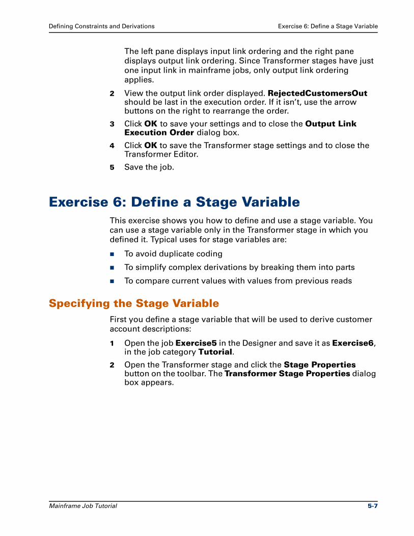
Defining Constraints and Derivations Exercise 6: Define a Stage Variable
The left pane displays input link ordering and the right pane
displays output link ordering. Since Transformer stages have just
one input link in mainframe jobs, only output link ordering
applies.
2 View the output link order displayed. RejectedCustomersOut should be last in the execution order. If it isn’t, use the arrow buttons on the right to rearrange the order.
3 Click OK to save your settings and to close the Output Link Execution Order dialog box.
4 Click OK to save the Transformer stage settings and to close the Transformer Editor.
5 Save the job.
Exercise 6: Define a Stage VariableThis exercise shows you how to define and use a stage variable. You
can use a stage variable only in the Transformer stage in which you
defined it. Typical uses for stage variables are:
To avoid duplicate coding
To simplify complex derivations by breaking them into parts
To compare current values with values from previous reads
Specifying the Stage VariableFirst you define a stage variable that will be used to derive customer
account descriptions:
1 Open the job Exercise5 in the Designer and save it as Exercise6, in the job category Tutorial.
2 Open the Transformer stage and click the Stage Properties button on the toolbar. The Transformer Stage Properties dialog box appears.
Mainframe Job Tutorial 5-7
Exercise 6: Define a Stage Variable Defining Constraints and Derivations
Click the Variables tab to move this page to the front:
3 Define the stage variable properties using the grid:
a Type AcctDescription in the Name column.
b Type ‘Unknown’ in the Initial Value column.
c Select Char from the SQL type drop-down list.
d Type 10 in the Precision column.
e Type 0 in the Scale column.
f Optionally type a description in the Description column.
4 Click OK to save your changes. You have defined the stage variable.
Any stage variables you declare are shown in a table in the right pane
of the Links area. Click the Show/Hide Stage Variables button in the
Transformer toolbar to display this table if it is not visible.
Creating the DerivationNext you create the derivation for AcctDescription:
1 Double-click the AcctDescription Derivation cell to open the Expression Editor.
2 Create the following expression for AcctDescription:
IF CustomersOut.ACCOUNT_TYPE = ‘B’ THEN‘BUSINESS’
ELSEIF CustomersOut.ACCOUNT_TYPE = ‘I’ THEN
‘INDIVIDUAL’ ELSE
5-8 Mainframe Job Tutorial
Defining Constraints and Derivations Exercise 6: Define a Stage Variable
IF CustomersOut.ACCOUNT_TYPE = ‘N’ THEN ‘INTERNAL’
ELSE ‘UNKNOWN’
END END
END
You can type the expression directly in the Expression syntax
box, or you can build it using the IF THEN ELSE function, which is
stored in the Logical folder under Built-in Routines. You’ll need
to nest three IF THEN ELSE statements to specify account
descriptions for all three account types:
a Double-click IF THEN ELSE to insert it into the Expression syntax box.
b Replace <BooleanExpression> with the ACCOUNT_TYPE column.
c Insert the = operator after the column name, then type ‘B’.
d Replace <Expression1> with ‘BUSINESS’.
e Replace <Expression2> with the next IF THEN ELSE function.
f Repeat steps b–e for accounts with type ‘I’ (‘INDIVIDUAL’).
g Repeat steps b–d for accounts with type ‘N’ (‘INTERNAL’), then replace <Expression2> with ‘UNKNOWN’.
3 Click OK to close the Expression Editor. You have finished creating the derivation for the stage variable.
Inserting Columns into Output LinksNow you insert a new column named ACCOUNT_DESCRIPTION
into two of your output links:
1 Right-click the ActiveCustomersOut link in the Links area to display the Transformer Editor shortcut menu. Select Insert New Column from the ActiveCustomersOut shortcut menu.
2 In the Meta Data area of the Transformer Editor, define the column as follows:
a Type ACCOUNT_DESCRIPTION in the Column name field.
b Select Char from the SQL type drop-down list.
c Type 10 in the Length field.
3 In the Links area, drag and drop the AcctDescription stage variable to the Derivation cell for the column.
4 Move the new column in the ActiveCustomersOut table so that it appears just after ACCOUNT_TYPE. Use drag-and-drop by clicking the ACCOUNT_DESCRIPTION Column Name cell and
Mainframe Job Tutorial 5-9
Exercise 7: Define a Job Parameter Defining Constraints and Derivations
dragging the mouse pointer to just under the ACCOUNT_TYPE cell. You will see an insert point that indicates where the column will be moved.
5 Repeat steps 1–4 to define the same column in the InactiveCustomersOut link.
6 Click OK to save your settings and to close the Transformer Editor.
Configuring Target StagesFinally you configure the two new Fixed-Width Flat File target stages:
1 Define the InactiveCustomers target stage:
a Type SLS.IACTCUST in the File name field.
b Type IACTCUST in the DD name field.
c Select Delete and recreate existing file as the write option. This means that if you run the job more than once, Ascential DataStage creates the JCL necessary to delete any existing file that has already been cataloged.
d Verify that the correct column definitions appear in the Columns grid.
2 Define the RejectedCustomers target stage:
a Type SLS.REJCUST in the File name field.
b Type REJCUST in the DD name field.
c Select Delete and recreate existing file as the write option.
d Verify the column definitions in the Columns grid.
3 Save the job.
You have finished defining the stage variable, using it in your output
column derivations, and configuring your target stages.
Exercise 7: Define a Job ParameterThe final exercise in this chapter has you define a job parameter. Job
parameters are processing variables used in constraints and column
derivations. They can save time by allowing you to customize a job
without having to reedit stages and regenerate code. For example,
you can filter the rows used for a job that produces a regional or
quarterly report by using a parameter to specify different territories or
dates. In the following exercise, you use a job parameter to specify
different credit ratings for different runs of the job.
5-10 Mainframe Job Tutorial
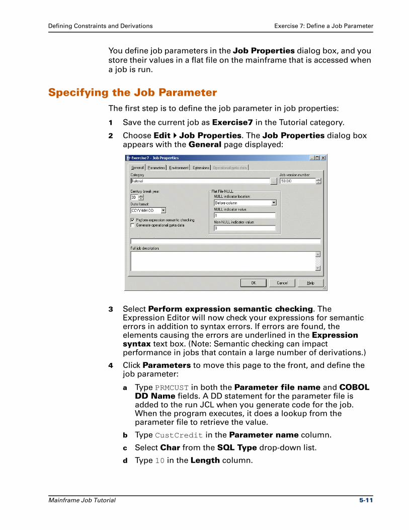
Defining Constraints and Derivations Exercise 7: Define a Job Parameter
You define job parameters in the Job Properties dialog box, and you
store their values in a flat file on the mainframe that is accessed when
a job is run.
Specifying the Job ParameterThe first step is to define the job parameter in job properties:
1 Save the current job as Exercise7 in the Tutorial category.
2 Choose Edit Job Properties. The Job Properties dialog box appears with the General page displayed:
3 Select Perform expression semantic checking. The Expression Editor will now check your expressions for semantic errors in addition to syntax errors. If errors are found, the elements causing the errors are underlined in the Expression syntax text box. (Note: Semantic checking can impact performance in jobs that contain a large number of derivations.)
4 Click Parameters to move this page to the front, and define the job parameter:
a Type PRMCUST in both the Parameter file name and COBOL DD Name fields. A DD statement for the parameter file is added to the run JCL when you generate code for the job. When the program executes, it does a lookup from the parameter file to retrieve the value.
b Type CustCredit in the Parameter name column.
c Select Char from the SQL Type drop-down list.
d Type 10 in the Length column.
Mainframe Job Tutorial 5-11
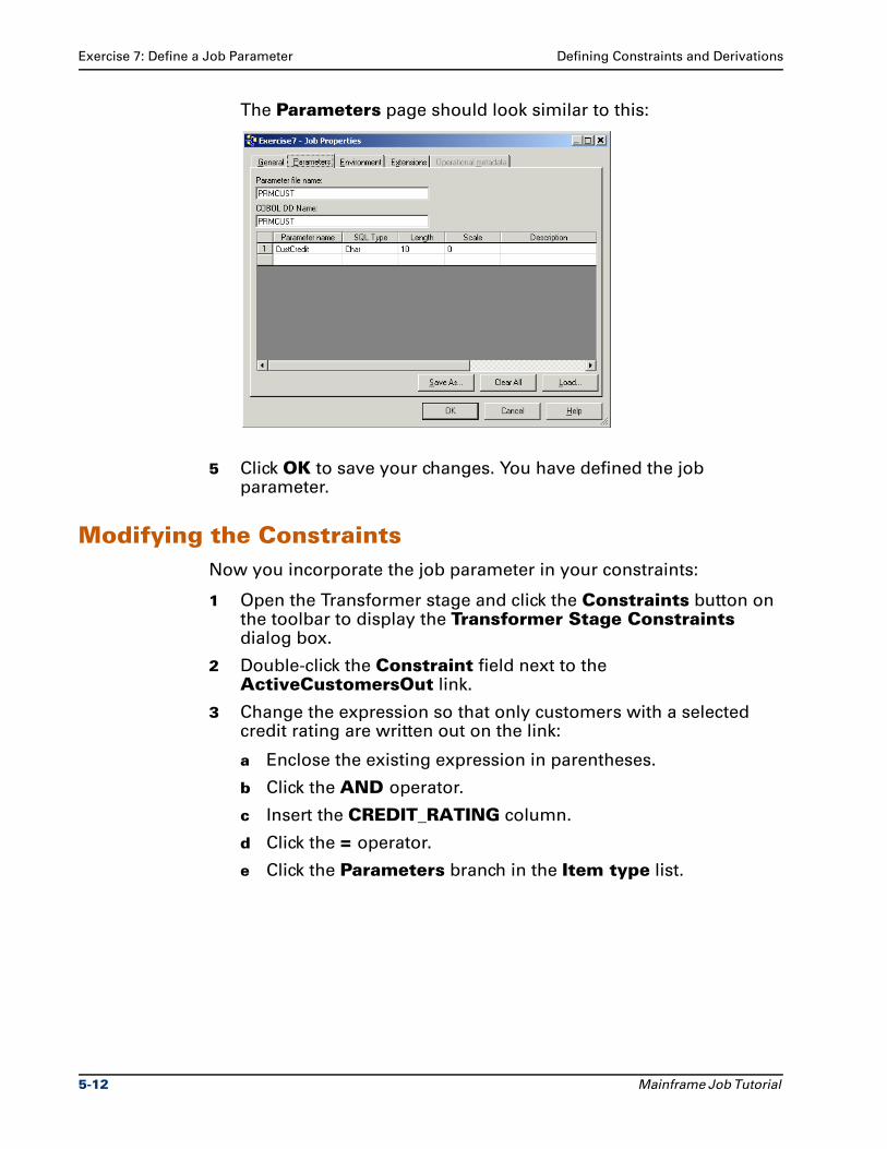
Exercise 7: Define a Job Parameter Defining Constraints and Derivations
The Parameters page should look similar to this:
5 Click OK to save your changes. You have defined the job parameter.
Modifying the ConstraintsNow you incorporate the job parameter in your constraints:
1 Open the Transformer stage and click the Constraints button on the toolbar to display the Transformer Stage Constraints dialog box.
2 Double-click the Constraint field next to the ActiveCustomersOut link.
3 Change the expression so that only customers with a selected credit rating are written out on the link:
a Enclose the existing expression in parentheses.
b Click the AND operator.
c Insert the CREDIT_RATING column.
d Click the = operator.
e Click the Parameters branch in the Item type list.
5-12 Mainframe Job Tutorial
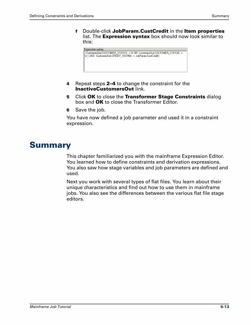
Defining Constraints and Derivations Summary
f Double-click JobParam.CustCredit in the Item properties list. The Expression syntax box should now look similar to this:
4 Repeat steps 2–4 to change the constraint for the InactiveCustomersOut link.
5 Click OK to close the Transformer Stage Constraints dialog box and OK to close the Transformer Editor.
6 Save the job.
You have now defined a job parameter and used it in a constraint
expression.
SummaryThis chapter familiarized you with the mainframe Expression Editor.
You learned how to define constraints and derivation expressions.
You also saw how stage variables and job parameters are defined and
used.
Next you work with several types of flat files. You learn about their
unique characteristics and find out how to use them in mainframe
jobs. You also see the differences between the various flat file stage
editors.
Mainframe Job Tutorial 5-13
6Working with Simple Flat Files
This chapter explores the details of working with simple flat files in
mainframe jobs. You will build on what you learned in the last chapter
by working with more advanced capabilities in Fixed-Width Flat File
stages. You will also become familiar with the unique features of
Delimited Flat File and DB2 Load Ready Flat File stages.
In Exercise 8 you design a job that selects employees who are eligible
to receive an annual bonus and calculates the bonus amount. It reads
data from a delimited flat file, transforms it, and loads it to a fixed-
width flat file. You test what you’ve learned so far by configuring the
three stages, specifying a constraint, and defining an output column
derivation. You also see how easy it is to save column definitions as a
table definition in the Repository.
In Exercise 9 you modify the job to calculate hiring bonuses for new
employees. You add a constraint to the source stage, practice defining
and using a stage variable in a Transformer stage, and learn how to
configure a DB2 Load Ready Flat File target stage. Finally, in Exercise
10 you add an FTP stage to the job design so you can transfer the
target file to another machine.
Simple Flat File Stage TypesMainframe files can have simple or complex data structures. Complex
data structures include GROUP, REDEFINES, OCCURS, and OCCURS
DEPENDING ON clauses. Simple flat files do not contain these
clauses. Ascential DataStage Enterprise MVS Edition provides three
types of simple flat file stage:
Fixed-Width Flat File
Mainframe Job Tutorial 6-1
Simple Flat File Stage Types Working with Simple Flat Files
Delimited Flat File
DB2 Load Ready Flat File
Following is a brief introduction to the characteristics of these three
stages.
Fixed-Width Flat File StagesFixed-Width Flat File stages are used to extract data from or write data
to a simple flat file. They can be used as either a source or a target. As
you saw in Exercise 4, you can limit the rows being read by the stage
by specifying starting and ending rows. You can also add an end-of-
data indicator to the file if you wish to perform special data
manipulation tasks after the last row is processed. What’s more, you
can pre-sort your source file before sending it to the next stage in the
job design. You can write data to multiple output links and can define
constraints to limit the data being output on each link.
Delimited Flat File StagesDelimited Flat File stages also can be used as either sources or
targets. They read data from or write data to a delimited flat file. You
specify the type of column and string delimiters to use when handling
this type of flat file data. When Delimited Flat File stages are used as a
source, you can specify starting and ending rows as well as add an
end-of-data indicator to the file. As a target, Delimited Flat File stages
are typically used to write data to databases on different platforms
(other than DB2 on OS/390 platforms). An FTP stage often follows a
Delimited Flat File target stage in a job design, specifying the
information needed to transfer the delimited flat file to the target
machine.
DB2 Load Ready Flat File StagesDB2 Load Ready Flat File stages are target stages only. They write
data to a fixed-width flat file or a delimited flat file that can be loaded
to DB2 5.1 or later. You specify the parameters needed to run the DB2
bulk loader utility and generate the necessary control file. Ascential
DataStage adds a step to the run JCL to invoke the DB2 bulk loader
facility on the machine where the program is running. An FTP stage
can be used in conjunction with DB2 Load Ready Flat File stages for
file transfer.
6-2 Mainframe Job Tutorial
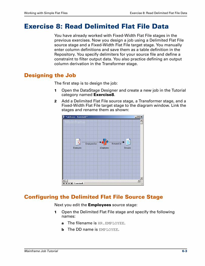
Working with Simple Flat Files Exercise 8: Read Delimited Flat File Data
Exercise 8: Read Delimited Flat File DataYou have already worked with Fixed-Width Flat File stages in the
previous exercises. Now you design a job using a Delimited Flat File
source stage and a Fixed-Width Flat File target stage. You manually
enter column definitions and save them as a table definition in the
Repository. You specify delimiters for your source file and define a
constraint to filter output data. You also practice defining an output
column derivation in the Transformer stage.
Designing the JobThe first step is to design the job:
1 Open the DataStage Designer and create a new job in the Tutorial category named Exercise8.
2 Add a Delimited Flat File source stage, a Transformer stage, and a Fixed-Width Flat File target stage to the diagram window. Link the stages and rename them as shown:
Configuring the Delimited Flat File Source StageNext you edit the Employees source stage:
1 Open the Delimited Flat File stage and specify the following names:
a The filename is HR.EMPLOYEE.
b The DD name is EMPLOYEE.
Mainframe Job Tutorial 6-3
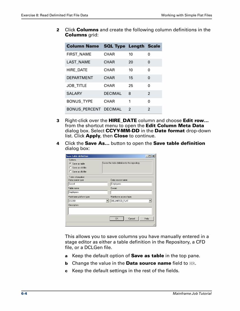
Exercise 8: Read Delimited Flat File Data Working with Simple Flat Files
2 Click Columns and create the following column definitions in the Columns grid:
3 Right-click over the HIRE_DATE column and choose Edit row… from the shortcut menu to open the Edit Column Meta Data dialog box. Select CCYY-MM-DD in the Date format drop-down list. Click Apply, then Close to continue.
4 Click the Save As… button to open the Save table definition dialog box:
This allows you to save columns you have manually entered in a
stage editor as either a table definition in the Repository, a CFD
file, or a DCLGen file.
a Keep the default option of Save as table in the top pane.
b Change the value in the Data source name field to HR.
c Keep the default settings in the rest of the fields.
Column Name SQL Type Length Scale
FIRST_NAME CHAR 10 0
LAST_NAME CHAR 20 0
HIRE_DATE CHAR 10 0
DEPARTMENT CHAR 15 0
JOB_TITLE CHAR 25 0
SALARY DECIMAL 8 2
BONUS_TYPE CHAR 1 0
BONUS_PERCENT DECIMAL 2 2
6-4 Mainframe Job Tutorial
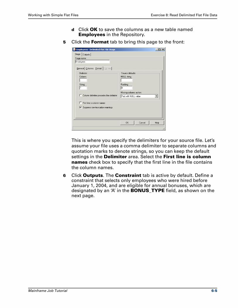
Working with Simple Flat Files Exercise 8: Read Delimited Flat File Data
d Click OK to save the columns as a new table named Employees in the Repository.
5 Click the Format tab to bring this page to the front:
This is where you specify the delimiters for your source file. Let’s
assume your file uses a comma delimiter to separate columns and
quotation marks to denote strings, so you can keep the default
settings in the Delimiter area. Select the First line is column names check box to specify that the first line in the file contains
the column names.
6 Click Outputs. The Constraint tab is active by default. Define a constraint that selects only employees who were hired before January 1, 2004, and are eligible for annual bonuses, which are designated by an ‘A’ in the BONUS_TYPE field, as shown on the next page.
Mainframe Job Tutorial 6-5
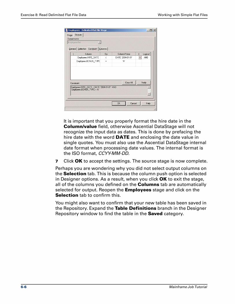
Exercise 8: Read Delimited Flat File Data Working with Simple Flat Files
It is important that you properly format the hire date in the
Column/value field, otherwise Ascential DataStage will not
recognize the input data as dates. This is done by prefacing the
hire date with the word DATE and enclosing the date value in
single quotes. You must also use the Ascential DataStage internal
date format when processing date values. The internal format is
the ISO format, CCYY-MM-DD.
7 Click OK to accept the settings. The source stage is now complete.
Perhaps you are wondering why you did not select output columns on
the Selection tab. This is because the column push option is selected
in Designer options. As a result, when you click OK to exit the stage,
all of the columns you defined on the Columns tab are automatically
selected for output. Reopen the Employees stage and click on the
Selection tab to confirm this.
You might also want to confirm that your new table has been saved in
the Repository. Expand the Table Definitions branch in the Designer
Repository window to find the table in the Saved category.
6-6 Mainframe Job Tutorial
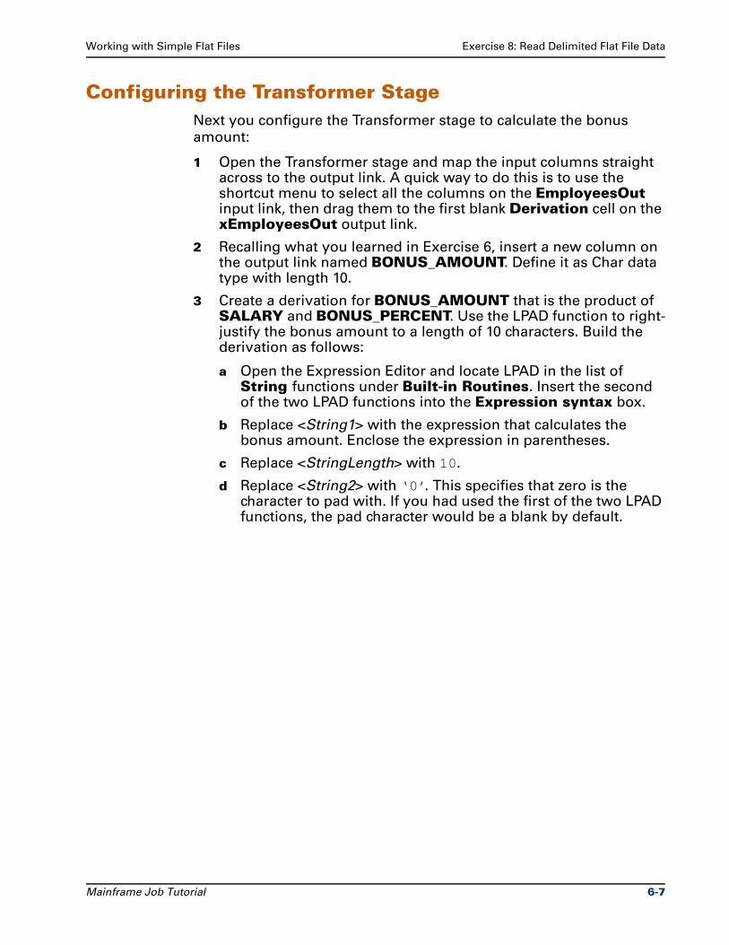
Working with Simple Flat Files Exercise 8: Read Delimited Flat File Data
Configuring the Transformer StageNext you configure the Transformer stage to calculate the bonus
amount:
1 Open the Transformer stage and map the input columns straight across to the output link. A quick way to do this is to use the shortcut menu to select all the columns on the EmployeesOut input link, then drag them to the first blank Derivation cell on the xEmployeesOut output link.
2 Recalling what you learned in Exercise 6, insert a new column on the output link named BONUS_AMOUNT. Define it as Char data type with length 10.
3 Create a derivation for BONUS_AMOUNT that is the product of SALARY and BONUS_PERCENT. Use the LPAD function to right-justify the bonus amount to a length of 10 characters. Build the derivation as follows:
a Open the Expression Editor and locate LPAD in the list of String functions under Built-in Routines. Insert the second of the two LPAD functions into the Expression syntax box.
b Replace <String1> with the expression that calculates the bonus amount. Enclose the expression in parentheses.
c Replace <StringLength> with 10.
d Replace <String2> with ‘0’. This specifies that zero is the character to pad with. If you had used the first of the two LPAD functions, the pad character would be a blank by default.
Mainframe Job Tutorial 6-7
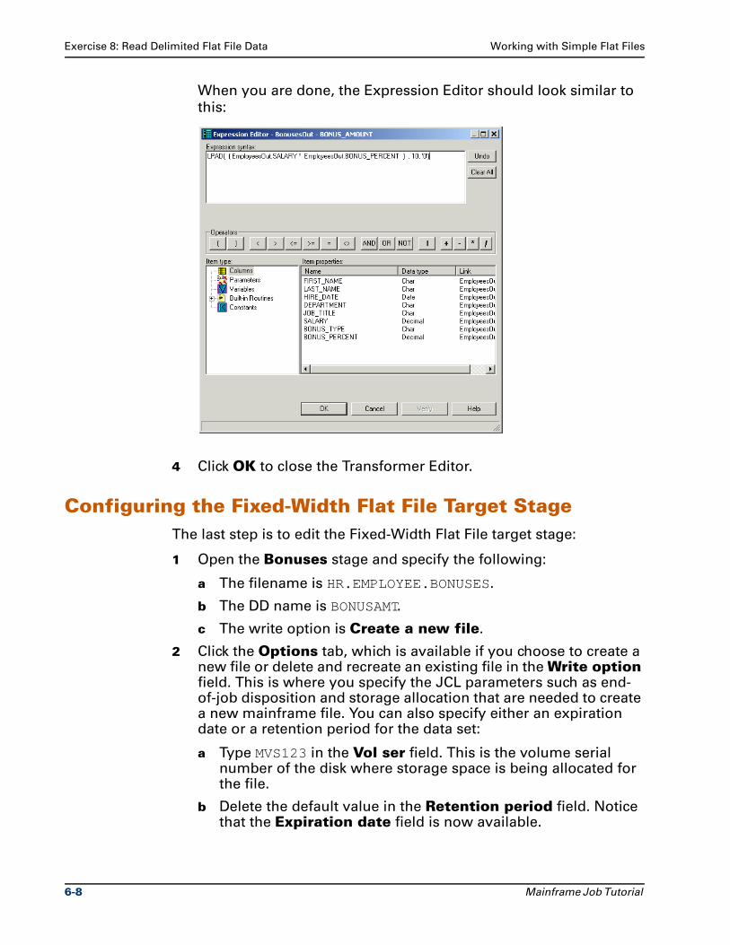
Exercise 8: Read Delimited Flat File Data Working with Simple Flat Files
When you are done, the Expression Editor should look similar to
this:
4 Click OK to close the Transformer Editor.
Configuring the Fixed-Width Flat File Target StageThe last step is to edit the Fixed-Width Flat File target stage:
1 Open the Bonuses stage and specify the following:
a The filename is HR.EMPLOYEE.BONUSES.
b The DD name is BONUSAMT.
c The write option is Create a new file.
2 Click the Options tab, which is available if you choose to create a new file or delete and recreate an existing file in the Write option field. This is where you specify the JCL parameters such as end-of-job disposition and storage allocation that are needed to create a new mainframe file. You can also specify either an expiration date or a retention period for the data set:
a Type MVS123 in the Vol ser field. This is the volume serial number of the disk where storage space is being allocated for the file.
b Delete the default value in the Retention period field. Notice that the Expiration date field is now available.
6-8 Mainframe Job Tutorial
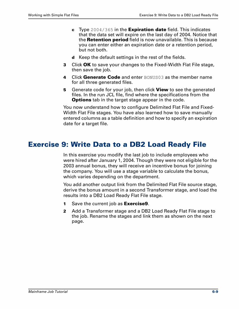
Working with Simple Flat Files Exercise 9: Write Data to a DB2 Load Ready File
c Type 2004/365 in the Expiration date field. This indicates that the data set will expire on the last day of 2004. Notice that the Retention period field is now unavailable. This is because you can enter either an expiration date or a retention period, but not both.
d Keep the default settings in the rest of the fields.
3 Click OK to save your changes to the Fixed-Width Flat File stage, then save the job.
4 Click Generate Code and enter BONUS03 as the member name for all three generated files.
5 Generate code for your job, then click View to see the generated files. In the run JCL file, find where the specifications from the Options tab in the target stage appear in the code.
You now understand how to configure Delimited Flat File and Fixed-
Width Flat File stages. You have also learned how to save manually
entered columns as a table definition and how to specify an expiration
date for a target file.
Exercise 9: Write Data to a DB2 Load Ready FileIn this exercise you modify the last job to include employees who
were hired after January 1, 2004. Though they were not eligible for the
2003 annual bonus, they will receive an incentive bonus for joining
the company. You will use a stage variable to calculate the bonus,
which varies depending on the department.
You add another output link from the Delimited Flat File source stage,
derive the bonus amount in a second Transformer stage, and load the
results into a DB2 Load Ready Flat File stage.
1 Save the current job as Exercise9.
2 Add a Transformer stage and a DB2 Load Ready Flat File stage to the job. Rename the stages and link them as shown on the next page.
Mainframe Job Tutorial 6-9
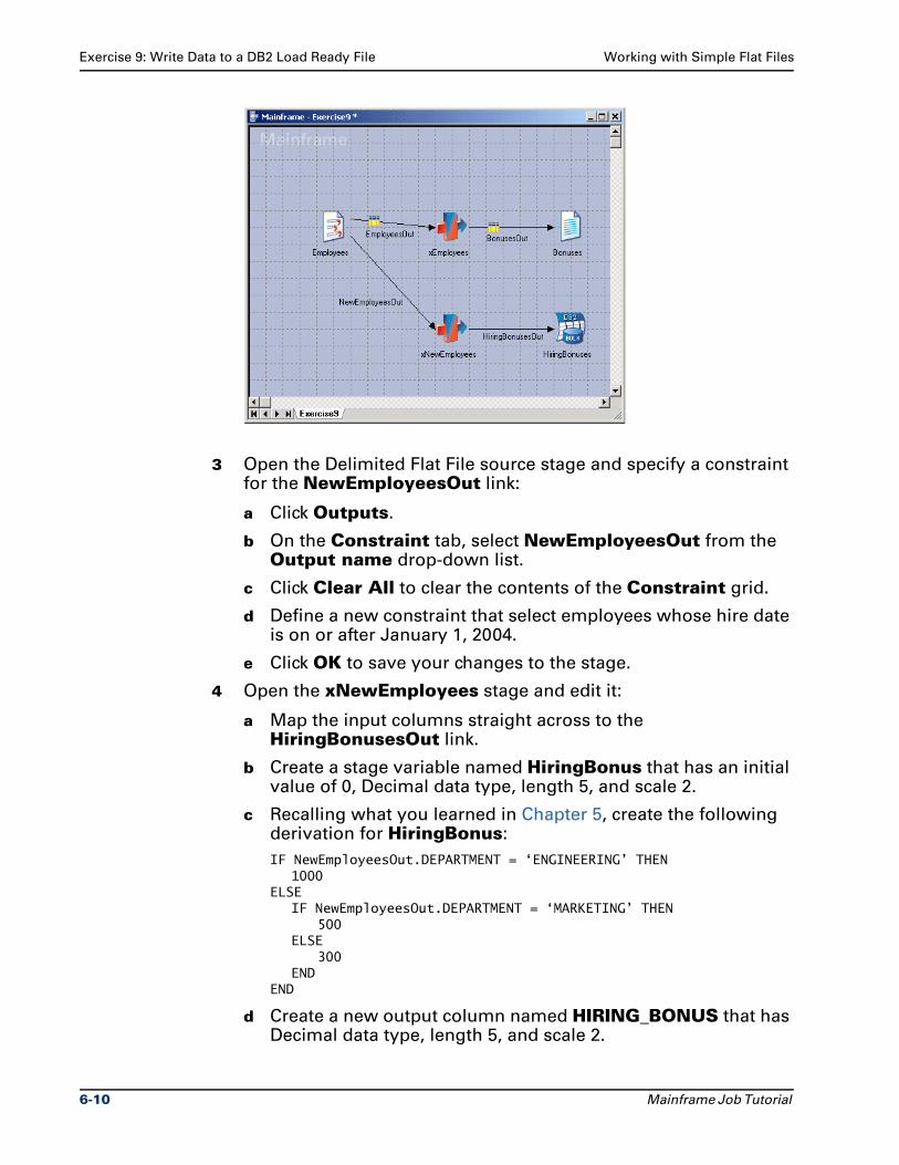
Exercise 9: Write Data to a DB2 Load Ready File Working with Simple Flat Files
3 Open the Delimited Flat File source stage and specify a constraint for the NewEmployeesOut link:
a Click Outputs.
b On the Constraint tab, select NewEmployeesOut from the Output name drop-down list.
c Click Clear All to clear the contents of the Constraint grid.
d Define a new constraint that select employees whose hire date is on or after January 1, 2004.
e Click OK to save your changes to the stage.
4 Open the xNewEmployees stage and edit it:
a Map the input columns straight across to the HiringBonusesOut link.
b Create a stage variable named HiringBonus that has an initial value of 0, Decimal data type, length 5, and scale 2.
c Recalling what you learned in Chapter 5, create the following derivation for HiringBonus:
IF NewEmployeesOut.DEPARTMENT = ‘ENGINEERING’ THEN 1000
ELSE IF NewEmployeesOut.DEPARTMENT = ‘MARKETING’ THEN
500 ELSE
300END
END
d Create a new output column named HIRING_BONUS that has Decimal data type, length 5, and scale 2.
6-10 Mainframe Job Tutorial
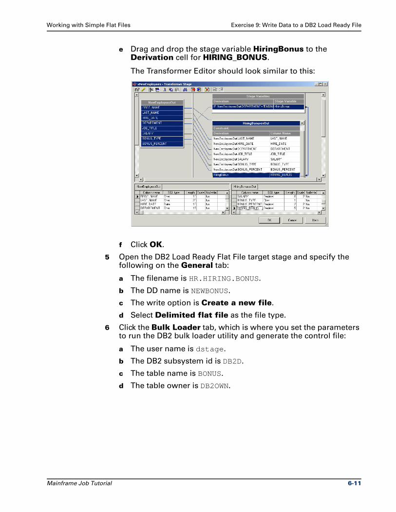
Working with Simple Flat Files Exercise 9: Write Data to a DB2 Load Ready File
e Drag and drop the stage variable HiringBonus to the Derivation cell for HIRING_BONUS.
The Transformer Editor should look similar to this:
f Click OK.
5 Open the DB2 Load Ready Flat File target stage and specify the following on the General tab:
a The filename is HR.HIRING.BONUS.
b The DD name is NEWBONUS.
c The write option is Create a new file.
d Select Delimited flat file as the file type.
6 Click the Bulk Loader tab, which is where you set the parameters to run the DB2 bulk loader utility and generate the control file:
a The user name is dstage.
b The DB2 subsystem id is DB2D.
c The table name is BONUS.
d The table owner is DB2OWN.
Mainframe Job Tutorial 6-11
Exercise 10: Use an FTP Stage Working with Simple Flat Files
7 Click the Format tab to specify delimiter information for the target file:
a Keep the default settings in the Column delimiter, String delimiter, and Decimal point fields.
b Select Always delimit string data to delimit all string fields in the target file. (If this box is not selected, then string fields are delimited only if the data contains the column delimiter character itself).
8 On the Options tab, specify the following:
a The volume serial number is MVS123.
b The database version is 6.1.
c The expiration date is 2004/365.
9 Click OK to save your changes.
10 Click Generate Code and enter BONUS04 as the member name for all three generated files. Generate code for the job and view the Run JCL to see how it differs from that of the last exercise.
Exercise 10: Use an FTP StageThe next step is to add an FTP stage to your job so you can transfer
the DB2 load ready file to another machine. FTP stages collect the
information needed to generate the JCL that is used to transfer the
file. They accept input from Delimited Flat File stages, DB2 Load
Ready Flat File stages, and Fixed-Width Flat File stages. They use
either FTP or Connect:Direct for file transfer.
1 Save the current job as Exercise10.
2 Add an FTP stage to the job and link it to the DB2 Load Ready Flat File stage. Rename the stage and link as shown on the next page.
6-12 Mainframe Job Tutorial
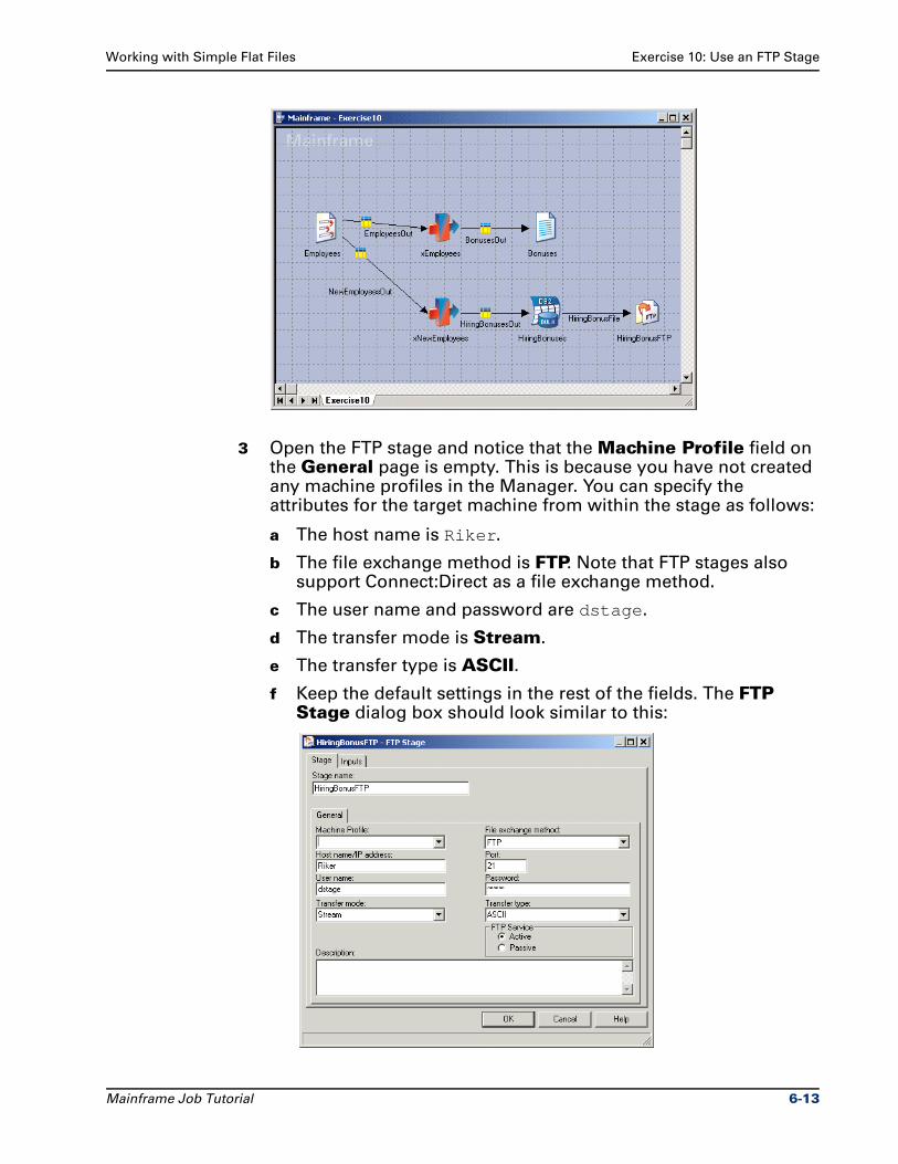
Working with Simple Flat Files Exercise 10: Use an FTP Stage
3 Open the FTP stage and notice that the Machine Profile field on the General page is empty. This is because you have not created any machine profiles in the Manager. You can specify the attributes for the target machine from within the stage as follows:
a The host name is Riker.
b The file exchange method is FTP. Note that FTP stages also support Connect:Direct as a file exchange method.
c The user name and password are dstage.
d The transfer mode is Stream.
e The transfer type is ASCII.
f Keep the default settings in the rest of the fields. The FTP Stage dialog box should look similar to this:
Mainframe Job Tutorial 6-13
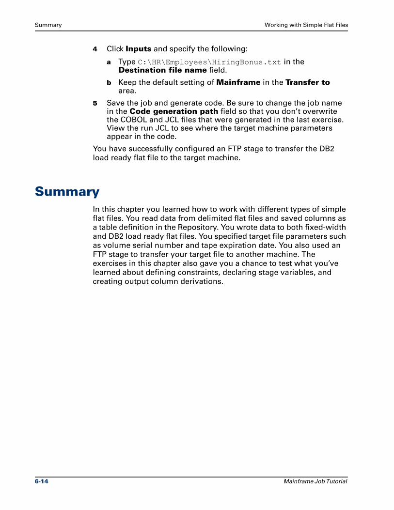
Summary Working with Simple Flat Files
4 Click Inputs and specify the following:
a Type C:\HR\Employees\HiringBonus.txt in the Destination file name field.
b Keep the default setting of Mainframe in the Transfer to area.
5 Save the job and generate code. Be sure to change the job name in the Code generation path field so that you don’t overwrite the COBOL and JCL files that were generated in the last exercise. View the run JCL to see where the target machine parameters appear in the code.
You have successfully configured an FTP stage to transfer the DB2
load ready flat file to the target machine.
SummaryIn this chapter you learned how to work with different types of simple
flat files. You read data from delimited flat files and saved columns as
a table definition in the Repository. You wrote data to both fixed-width
and DB2 load ready flat files. You specified target file parameters such
as volume serial number and tape expiration date. You also used an
FTP stage to transfer your target file to another machine. The
exercises in this chapter also gave you a chance to test what you’ve
learned about defining constraints, declaring stage variables, and
creating output column derivations.
6-14 Mainframe Job Tutorial
7Working with Complex Flat Files
You have worked with simple flat files in mainframe jobs. Now you
see how to read data from complex flat files. Ascential DataStage
Enterprise MVS Edition has two complex flat file stage types: Complex
Flat File and Multi-Format Flat File. The exercises in this chapter show
you how to configure them as sources and manipulate their complex
data structures.
In Exercise 11 you create a job that provides information about several
products in a product line. It extracts data from a complex flat file,
transforms it, and loads it to a delimited flat file. You practice what
you’ve learned so far by configuring the three stages, specifying a job
parameter, and defining a constraint. You also see how easy it is to
convert dates from one format to another.
Exercise 12 takes you a step further with complex flat files by showing
you how to flatten an array. You manipulate the flattened data to
create an output file that lists product colors. At the end of each
exercise you generate code for the job and look at the results.
In Exercise 13 you learn about OCCURS DEPENDING ON clauses. You
design a job that flattens an array containing product discount
information. Your then create an output file that indicates whether a
product discount is in effect as of the current date. As part of this, you
define and use stage variables.
Exercise 14 introduces you to multi-format flat files. You create a job
that reads variable-length records from a purchase order file and
writes them to three DB2 load ready target files. You also practice
importing table definitions in the Manager. In Exercise 15, you see
how to merge multiple record types down a single output link.
Mainframe Job Tutorial 7-1
Complex Flat File Stage Types Working with Complex Flat Files
Complex Flat File Stage TypesComplex flat files contain COBOL clauses such as GROUP,
REDEFINES, OCCURS, or OCCURS DEPENDING ON clauses. They can
have fixed or variable record lengths. You can extract data from
complex flat file data structures using the following stage types:
Complex Flat File
Multi-Format Flat File
Before starting the exercises, it will be helpful to understand the
differences between these stages and how they are used.
Complex Flat File StagesComplex Flat File stages can read the following types of complex flat
file:
QSAM_SEQ_COMPLEX. QSAM file structures.
VSAM_ESDS. VSAM Entry Sequenced Data Set file structures, from which records are read sequentially.
VSAM_KSDS. VSAM Key-Sequenced Data Set file structures, from which records are read using a key.
VSAM_RRDS. VSAM Relative Record Data Set file structures, from which records are read using a relative number.
Complex Flat File stages can be used to read data from files
containing fixed or variable record lengths. When you load a CFD
containing arrays, you can choose to normalize, flatten, or selectively
flatten the arrays. You will work with arrays later in this chapter.
As with Fixed-Width Flat File stages, you can limit the rows being read
by the stage, add an end-of-data indicator, and pre-sort the source file.
You can also define a constraint to limit output data, and you can write
data to multiple output links.
Multi-Format Flat File StagesMulti-Format Flat File stages are typically used to extract data from
files whose record lengths vary based on multiple record types.
However, they can also read data from files containing fixed record
lengths. They read the same four types of file structure as Complex
Flat File stages. The source data may contain one or more GROUP,
REDEFINES, OCCURS, or OCCURS DEPENDING ON clauses per
record type.
7-2 Mainframe Job Tutorial
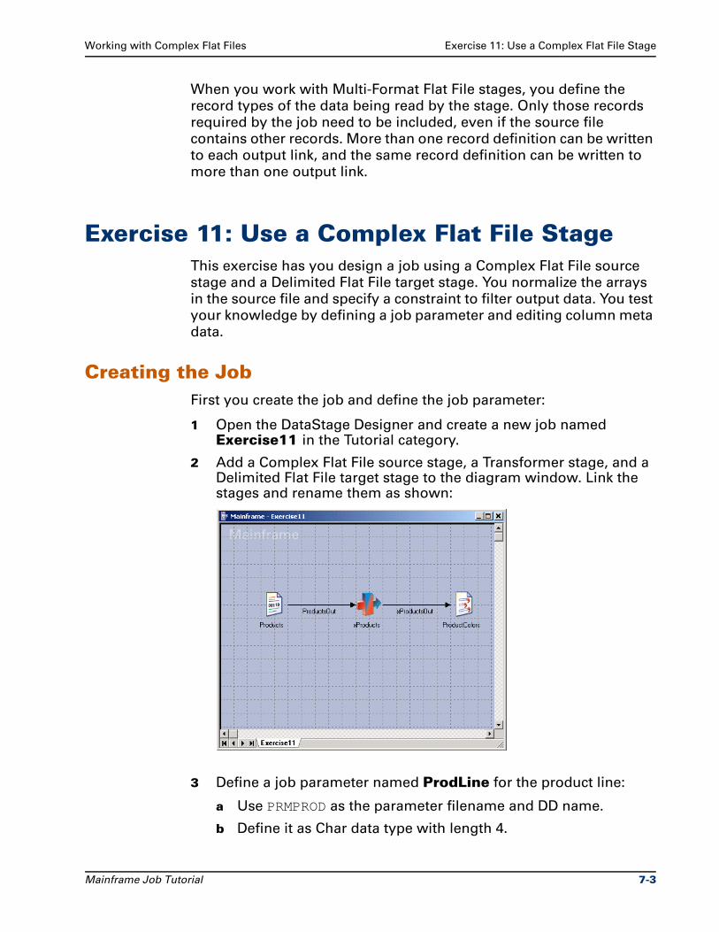
Working with Complex Flat Files Exercise 11: Use a Complex Flat File Stage
When you work with Multi-Format Flat File stages, you define the
record types of the data being read by the stage. Only those records
required by the job need to be included, even if the source file
contains other records. More than one record definition can be written
to each output link, and the same record definition can be written to
more than one output link.
Exercise 11: Use a Complex Flat File StageThis exercise has you design a job using a Complex Flat File source
stage and a Delimited Flat File target stage. You normalize the arrays
in the source file and specify a constraint to filter output data. You test
your knowledge by defining a job parameter and editing column meta
data.
Creating the JobFirst you create the job and define the job parameter:
1 Open the DataStage Designer and create a new job named Exercise11 in the Tutorial category.
2 Add a Complex Flat File source stage, a Transformer stage, and a Delimited Flat File target stage to the diagram window. Link the stages and rename them as shown:
3 Define a job parameter named ProdLine for the product line:
a Use PRMPROD as the parameter filename and DD name.
b Define it as Char data type with length 4.
Mainframe Job Tutorial 7-3
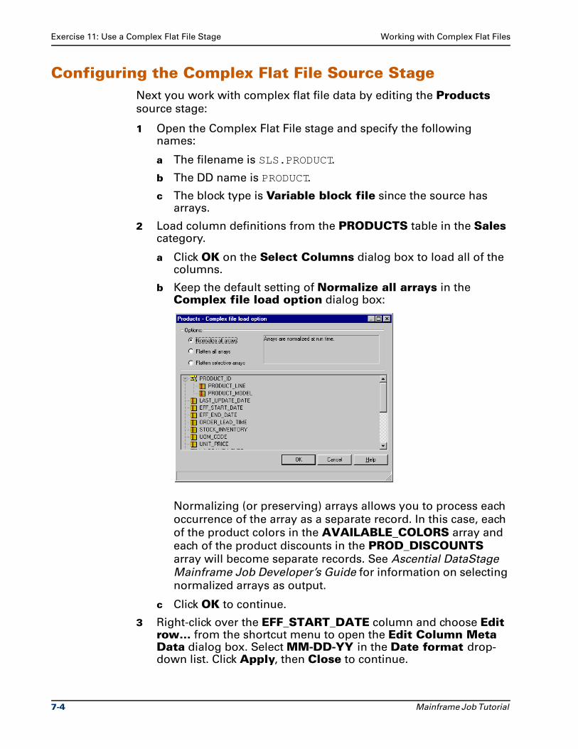
Exercise 11: Use a Complex Flat File Stage Working with Complex Flat Files
Configuring the Complex Flat File Source StageNext you work with complex flat file data by editing the Products
source stage:
1 Open the Complex Flat File stage and specify the following names:
a The filename is SLS.PRODUCT.
b The DD name is PRODUCT.
c The block type is Variable block file since the source has arrays.
2 Load column definitions from the PRODUCTS table in the Sales category.
a Click OK on the Select Columns dialog box to load all of the columns.
b Keep the default setting of Normalize all arrays in the Complex file load option dialog box:
Normalizing (or preserving) arrays allows you to process each
occurrence of the array as a separate record. In this case, each
of the product colors in the AVAILABLE_COLORS array and
each of the product discounts in the PROD_DISCOUNTS
array will become separate records. See Ascential DataStage
Mainframe Job Developer’s Guide for information on selecting
normalized arrays as output.
c Click OK to continue.
3 Right-click over the EFF_START_DATE column and choose Edit row… from the shortcut menu to open the Edit Column Meta Data dialog box. Select MM-DD-YY in the Date format drop-down list. Click Apply, then Close to continue.
7-4 Mainframe Job Tutorial
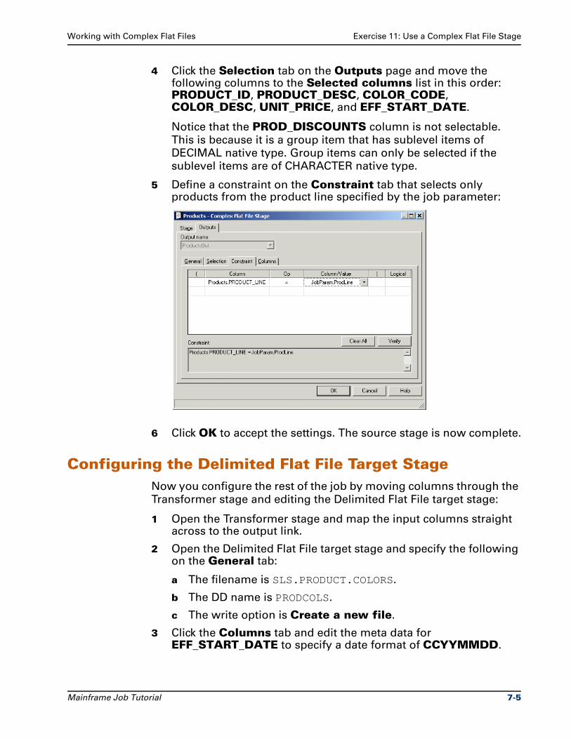
Working with Complex Flat Files Exercise 11: Use a Complex Flat File Stage
4 Click the Selection tab on the Outputs page and move the following columns to the Selected columns list in this order: PRODUCT_ID, PRODUCT_DESC, COLOR_CODE, COLOR_DESC, UNIT_PRICE, and EFF_START_DATE.
Notice that the PROD_DISCOUNTS column is not selectable.
This is because it is a group item that has sublevel items of
DECIMAL native type. Group items can only be selected if the
sublevel items are of CHARACTER native type.
5 Define a constraint on the Constraint tab that selects only products from the product line specified by the job parameter:
6 Click OK to accept the settings. The source stage is now complete.
Configuring the Delimited Flat File Target StageNow you configure the rest of the job by moving columns through the
Transformer stage and editing the Delimited Flat File target stage:
1 Open the Transformer stage and map the input columns straight across to the output link.
2 Open the Delimited Flat File target stage and specify the following on the General tab:
a The filename is SLS.PRODUCT.COLORS.
b The DD name is PRODCOLS.
c The write option is Create a new file.
3 Click the Columns tab and edit the meta data for EFF_START_DATE to specify a date format of CCYYMMDD.
Mainframe Job Tutorial 7-5
Exercise 12: Flatten an Array Working with Complex Flat Files
Ascential DataStage Enterprise MVS Edition makes it easy to
convert dates from one format to another when moving data from
a source to a target. You select the appropriate format in the
source and target stages using the Edit Column Meta Data dialog box. When you generate code, the date is converted to the
new format automatically.
4 Click the Format tab and specify a pipe (|) as the column delimiter.
5 Click the Options tab and specify MVS123 as the volume serial number and 180 as the retention period.
6 Click OK to save your changes to the Delimited Flat File stage, then save the job.
7 Click Generate Code and enter PRODCOL as the member name for all three generated files.
8 Generate code for your job, then click View to see the generated files.
At this point, you are familiar with how to configure Complex Flat File
stages. You understand how to read data from complex file structures
and what happens when you normalize arrays. You have also seen
how to use a Delimited Flat File stage as a target.
Exercise 12: Flatten an ArrayLet’s expand on what you learned in Exercise 11 by flattening an array.
When an array is flattened, each occurrence (as noted by the OCCURS
clause in the input file) becomes a separate column. When a row is
read from the file, all occurrences of the array are flattened into a
single row.
1 Open the job Exercise11 and save it as Exercise12.
2 Open the Complex Flat File stage and modify the stage so that each product is listed only once in the output file along with a list of its colors:
a Clear the column definitions on the Columns tab and reload all of the column definitions from the PRODUCTS table.
b Click Flatten selective arrays on the Complex file load option dialog box, then right-click the AVAILABLE_COLORS array and select Flatten. Notice that the array icon changes. Each occurrence of AVAILABLE_COLORS will now become a separate column. Click OK to continue.
7-6 Mainframe Job Tutorial
Working with Complex Flat Files Exercise 12: Flatten an Array
c Click the Selection tab on the Outputs page and scroll down the Available columns list. Notice that AVAILABLE_ COLORS appears four times, with a suffix showing the occurrence number.
d Modify the Selected columns list on the Selection tab to include the following columns: PRODUCT_ID, PRODUCT_DESC, COLOR_DESC, COLOR_DESC_2, COLOR_DESC_3, COLOR_DESC_4, UNIT_PRICE, and EFF_START_DATE. Use the arrow buttons to the right of the Selected columns list to arrange the columns in this order.
e Do not change the constraint on the Constraint tab.
f Click OK to save your changes to the source stage.
3 Open the Delimited Flat File target stage and change the filename on the General tab to SLS.PRODUCT.COLORS.LIST. Delete the COLOR_CODE column on the Columns tab.
4 Open the Transformer Stage and edit the COLOR_DESC column derivation so that it results in a string of the form:
‘This product comes in colors: <color1>, <color2>, <color3> and <color4>’
To build the expression, use the color description input columns,
the concatenate (||) operator, and the trim function in the
Expression Editor as follows:
a In the Expression syntax box, clear the existing derivation and type:
‘This product comes in colors: ’
b Click the || operator. This joins the initial text string with the next component of the expression.
c Since the length of the color descriptions varies, you want to trim any blank spaces to make the result more readable. Expand the Built-in Routines branch of the Item type list. Click String to display the string functions. Double-click the TRIM function that trims trailing characters from a string.
d In the Expression syntax box, replace <Character> with ‘ ‘ (single quote, space, single quote). This specifies that the spaces are to be trimmed from the color description.
e In the Expression syntax box, highlight <String> and replace it with the COLOR_DESC column. This inserts the first color into the expression.
f Insert the || operator at the end of the expression.
g Type ‘, ’ to insert a comma and space after the first color.
Mainframe Job Tutorial 7-7
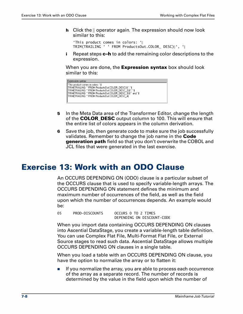
Exercise 13: Work with an ODO Clause Working with Complex Flat Files
h Click the || operator again. The expression should now look similar to this:
‘This product comes in colors: ‘|| TRIM(TRAILING ‘ ‘ FROM ProductsOut.COLOR_ DESC)||‘, ‘||
i Repeat steps c–h to add the remaining color descriptions to the expression.
When you are done, the Expression syntax box should look
similar to this:
5 In the Meta Data area of the Transformer Editor, change the length of the COLOR_DESC output column to 100. This will ensure that the entire list of colors appears in the column derivation.
6 Save the job, then generate code to make sure the job successfully validates. Remember to change the job name in the Code generation path field so that you don’t overwrite the COBOL and JCL files that were generated in the last exercise.
Exercise 13: Work with an ODO ClauseAn OCCURS DEPENDING ON (ODO) clause is a particular subset of
the OCCURS clause that is used to specify variable-length arrays. The
OCCURS DEPENDING ON statement defines the minimum and
maximum number of occurrences of the field, as well as the field
upon which the number of occurrences depends. An example would
be:
05 PROD-DISCOUNTS OCCURS 0 TO 2 TIMESDEPENDING ON DISCOUNT-CODE
When you import data containing OCCURS DEPENDING ON clauses
into Ascential DataStage, you create a variable-length table definition.
You can use Complex Flat File, Multi-Format Flat File, or External
Source stages to read such data. Ascential DataStage allows multiple
OCCURS DEPENDING ON clauses in a single table.
When you load a table with an OCCURS DEPENDING ON clause, you
have the option to normalize the array or to flatten it:
If you normalize the array, you are able to process each occurrence of the array as a separate record. The number of records is determined by the value in the field upon which the number of
7-8 Mainframe Job Tutorial
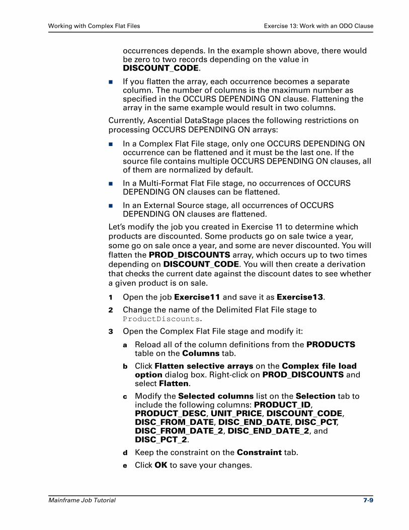
Working with Complex Flat Files Exercise 13: Work with an ODO Clause
occurrences depends. In the example shown above, there would be zero to two records depending on the value in DISCOUNT_CODE.
If you flatten the array, each occurrence becomes a separate column. The number of columns is the maximum number as specified in the OCCURS DEPENDING ON clause. Flattening the array in the same example would result in two columns.
Currently, Ascential DataStage places the following restrictions on
processing OCCURS DEPENDING ON arrays:
In a Complex Flat File stage, only one OCCURS DEPENDING ON occurrence can be flattened and it must be the last one. If the source file contains multiple OCCURS DEPENDING ON clauses, all of them are normalized by default.
In a Multi-Format Flat File stage, no occurrences of OCCURS DEPENDING ON clauses can be flattened.
In an External Source stage, all occurrences of OCCURS DEPENDING ON clauses are flattened.
Let’s modify the job you created in Exercise 11 to determine which
products are discounted. Some products go on sale twice a year,
some go on sale once a year, and some are never discounted. You will
flatten the PROD_DISCOUNTS array, which occurs up to two times
depending on DISCOUNT_CODE. You will then create a derivation
that checks the current date against the discount dates to see whether
a given product is on sale.
1 Open the job Exercise11 and save it as Exercise13.
2 Change the name of the Delimited Flat File stage to ProductDiscounts.
3 Open the Complex Flat File stage and modify it:
a Reload all of the column definitions from the PRODUCTS table on the Columns tab.
b Click Flatten selective arrays on the Complex file load option dialog box. Right-click on PROD_DISCOUNTS and select Flatten.
c Modify the Selected columns list on the Selection tab to include the following columns: PRODUCT_ID, PRODUCT_DESC, UNIT_PRICE, DISCOUNT_CODE, DISC_FROM_DATE, DISC_END_DATE, DISC_PCT, DISC_FROM_DATE_2, DISC_END_DATE_2, and DISC_PCT_2.
d Keep the constraint on the Constraint tab.
e Click OK to save your changes.
Mainframe Job Tutorial 7-9
Exercise 13: Work with an ODO Clause Working with Complex Flat Files
4 Open the Transformer stage and modify it:
a Delete the columns COLOR_CODE, COLOR_DESC, and EFF_START_DATE from the output link.
b Insert a new column named DISCOUNT on the output link. Define it as Decimal data type with length 3 and scale 3.
c Recalling what you learned in Chapter 5, create four stage variables named DiscountStartDate1, DiscountEndDate1, DiscountStartDate2, and DiscountEndDate2. Specify Date SQL type and precision 10 for each variable.
d Create derivations for the stage variables to convert the columns DISC_FROM_DATE, DISC_END_DATE, DISC_FROM_DATE_2, and DISC_END_DATE_2 from Char to Date data type. (This is necessary for comparing dates, as you’ll see later.) To build the expressions, select the appropriate CAST function from the Data type Conversion branch of the Built-in Routines list. When you are done, the Stage Variables table in the Transformer Editor should look similar to this:
e Create a derivation for DISCOUNT that compares today’s date with the discount dates and returns the applicable discount percent, if any. To build the expression, use a series of nested IF THEN ELSE statements. First you must check the value in DISCOUNT_CODE (which can be 0, 1, or 2) to find out how many times a product goes on sale. Remember that the number of occurrences of the PROD_DISCOUNTS array depends on the value in DISCOUNT_CODE. Once you determine the number of times a product goes on sale, you know whether to check today’s date against one or both of the discount periods.
For example, if DISCOUNT_CODE is 0, then the product
never goes on sale and the expression returns a value of 0. If
DISCOUNT_CODE is 1, then the product is discounted during
the first sale. The expression checks to see if today’s date falls
within the sale dates. If so, then the expression returns the
discount percent. If not, it returns a value of 0. Similarly, if
DISCOUNT_CODE is 2, then the product is discounted during
7-10 Mainframe Job Tutorial
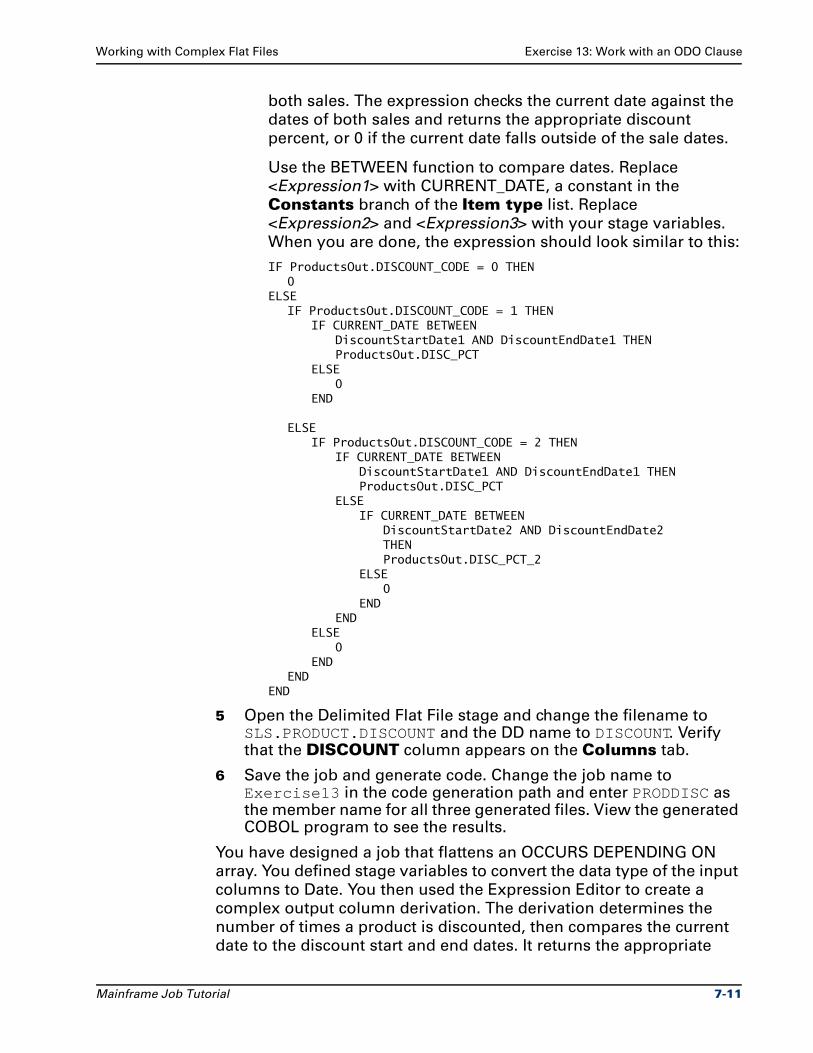
Working with Complex Flat Files Exercise 13: Work with an ODO Clause
both sales. The expression checks the current date against the
dates of both sales and returns the appropriate discount
percent, or 0 if the current date falls outside of the sale dates.
Use the BETWEEN function to compare dates. Replace
<Expression1> with CURRENT_DATE, a constant in the
Constants branch of the Item type list. Replace
<Expression2> and <Expression3> with your stage variables.
When you are done, the expression should look similar to this:
IF ProductsOut.DISCOUNT_CODE = 0 THEN 0
ELSEIF ProductsOut.DISCOUNT_CODE = 1 THEN
IF CURRENT_DATE BETWEEN DiscountStartDate1 AND DiscountEndDate1 THENProductsOut.DISC_PCT
ELSE 0
END
ELSEIF ProductsOut.DISCOUNT_CODE = 2 THEN
IF CURRENT_DATE BETWEEN DiscountStartDate1 AND DiscountEndDate1 THENProductsOut.DISC_PCT
ELSE IF CURRENT_DATE BETWEEN
DiscountStartDate2 AND DiscountEndDate2THEN ProductsOut.DISC_PCT_2
ELSE 0
END END
ELSE0
END END
END
5 Open the Delimited Flat File stage and change the filename to SLS.PRODUCT.DISCOUNT and the DD name to DISCOUNT. Verify that the DISCOUNT column appears on the Columns tab.
6 Save the job and generate code. Change the job name to Exercise13 in the code generation path and enter PRODDISC as the member name for all three generated files. View the generated COBOL program to see the results.
You have designed a job that flattens an OCCURS DEPENDING ON
array. You defined stage variables to convert the data type of the input
columns to Date. You then used the Expression Editor to create a
complex output column derivation. The derivation determines the
number of times a product is discounted, then compares the current
date to the discount start and end dates. It returns the appropriate
Mainframe Job Tutorial 7-11
Exercise 14: Use a Multi-Format Flat File Stage Working with Complex Flat Files
discount percent if a product is on sale or zero if the product is not on
sale.
Exercise 14: Use a Multi-Format Flat File StageThis exercise shows you how to read data from a file containing
multiple record types. You import a CFD file containing different
records used for purchase orders. The three record types include a
customer record, an order record, and an invoice record. You design a
job using a Multi-Format Flat File stage to read the source data and
three DB2 Load Ready stages to bulk load the data to the target DB2
tables.
Import the Record DefinitionsThe first step is to import the multi-format file definition and look at
the record types:
1 Open the Manager and import the MCUST_REC, MINV_REC, and MORD_REC record definitions from the PurchaseOrders.cfd file on the tutorial CD, recalling what you learned in Chapter 3. Save the record definitions in the COBOL FD\Sales category.
2 Open each of the three record definitions and look at the column meta data. The column meta data for records in multi-format files is the same as that of other source file types. However, it is important to know the storage length of the largest record in the file, regardless of whether it will be used in the job. See if you can determine which record is the largest. You will use this information later.
Design the JobNext you design a job using a Multi-Format Flat File source stage with
three output link. Each output link handles data from one of the record
types in the multi-format file. The data on each link is then passed
through a Transformer stage and written to a DB2 Load Ready target
stage.
1 Open the Designer and create a new job in the Tutorial category named Exercise14.
2 Add a Multi-Format Flat File source stage, three Transformer stages, and three DB2 Load Ready target stages to the diagram window. Link the stages and rename them as shown:
7-12 Mainframe Job Tutorial
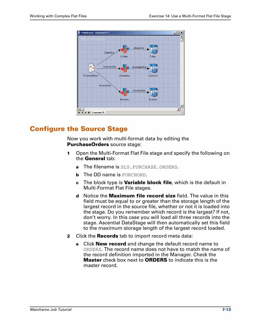
Working with Complex Flat Files Exercise 14: Use a Multi-Format Flat File Stage
Configure the Source StageNow you work with multi-format data by editing the
PurchaseOrders source stage:
1 Open the Multi-Format Flat File stage and specify the following on the General tab:
a The filename is SLS.PURCHASE.ORDERS.
b The DD name is PURCHORD.
c The block type is Variable block file, which is the default in Multi-Format Flat File stages.
d Notice the Maximum file record size field. The value in this field must be equal to or greater than the storage length of the largest record in the source file, whether or not it is loaded into the stage. Do you remember which record is the largest? If not, don’t worry. In this case you will load all three records into the stage. Ascential DataStage will then automatically set this field to the maximum storage length of the largest record loaded.
2 Click the Records tab to import record meta data:
e Click New record and change the default record name to ORDERS. The record name does not have to match the name of the record definition imported in the Manager. Check the Master check box next to ORDERS to indicate this is the master record.
Mainframe Job Tutorial 7-13
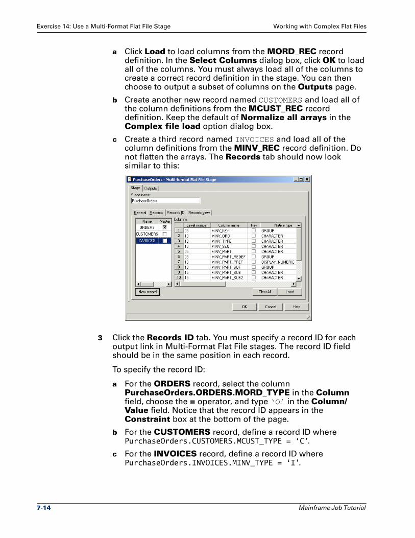
Exercise 14: Use a Multi-Format Flat File Stage Working with Complex Flat Files
a Click Load to load columns from the MORD_REC record definition. In the Select Columns dialog box, click OK to load all of the columns. You must always load all of the columns to create a correct record definition in the stage. You can then choose to output a subset of columns on the Outputs page.
b Create another new record named CUSTOMERS and load all of the column definitions from the MCUST_REC record definition. Keep the default of Normalize all arrays in the Complex file load option dialog box.
c Create a third record named INVOICES and load all of the column definitions from the MINV_REC record definition. Do not flatten the arrays. The Records tab should now look similar to this:
3 Click the Records ID tab. You must specify a record ID for each output link in Multi-Format Flat File stages. The record ID field should be in the same position in each record.
To specify the record ID:
a For the ORDERS record, select the column PurchaseOrders.ORDERS.MORD_TYPE in the Column field, choose the = operator, and type ‘O’ in the Column/Value field. Notice that the record ID appears in the Constraint box at the bottom of the page.
b For the CUSTOMERS record, define a record ID where PurchaseOrders.CUSTOMERS.MCUST_TYPE = ‘C’.
c For the INVOICES record, define a record ID where PurchaseOrders.INVOICES.MINV_TYPE = ‘I’.
7-14 Mainframe Job Tutorial
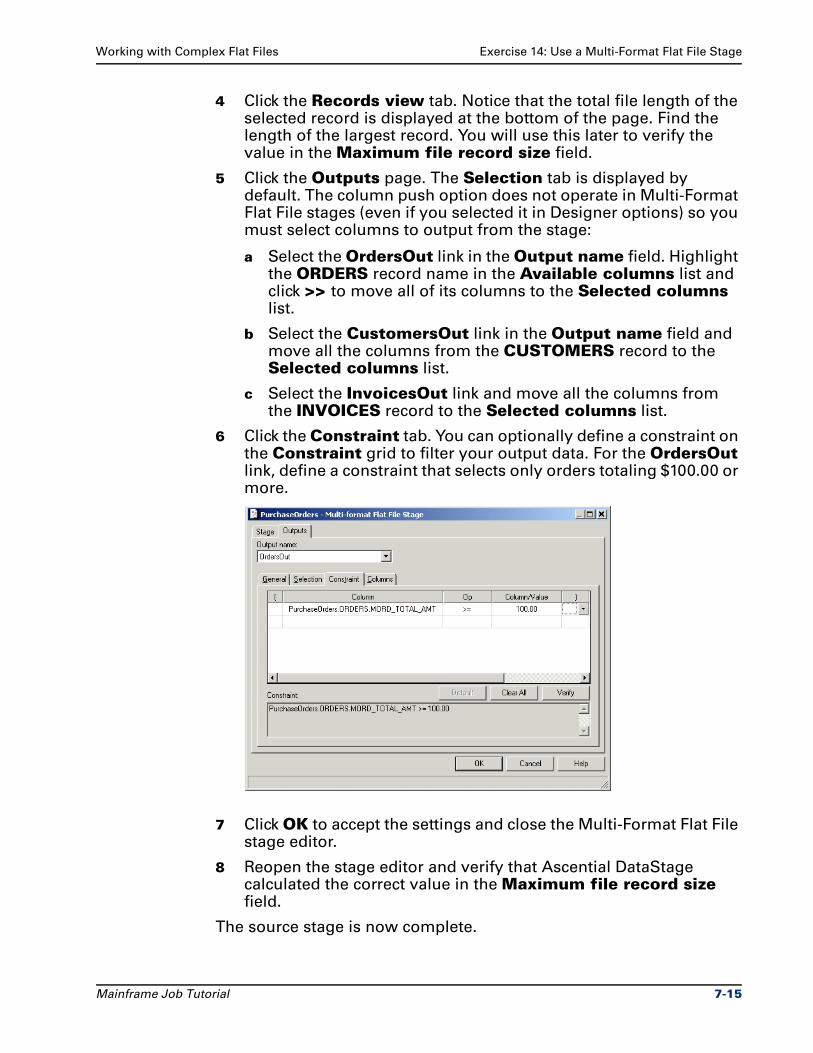
Working with Complex Flat Files Exercise 14: Use a Multi-Format Flat File Stage
4 Click the Records view tab. Notice that the total file length of the selected record is displayed at the bottom of the page. Find the length of the largest record. You will use this later to verify the value in the Maximum file record size field.
5 Click the Outputs page. The Selection tab is displayed by default. The column push option does not operate in Multi-Format Flat File stages (even if you selected it in Designer options) so you must select columns to output from the stage:
a Select the OrdersOut link in the Output name field. Highlight the ORDERS record name in the Available columns list and click >> to move all of its columns to the Selected columns list.
b Select the CustomersOut link in the Output name field and move all the columns from the CUSTOMERS record to the Selected columns list.
c Select the InvoicesOut link and move all the columns from the INVOICES record to the Selected columns list.
6 Click the Constraint tab. You can optionally define a constraint on the Constraint grid to filter your output data. For the OrdersOut link, define a constraint that selects only orders totaling $100.00 or more.
7 Click OK to accept the settings and close the Multi-Format Flat File stage editor.
8 Reopen the stage editor and verify that Ascential DataStage calculated the correct value in the Maximum file record size field.
The source stage is now complete.
Mainframe Job Tutorial 7-15
Exercise 14: Use a Multi-Format Flat File Stage Working with Complex Flat Files
Configure the Transformer and Target StagesNext you configure the rest of the job:
1 For each Transformer stage, map the input columns straight across to the output link. There’s an easy way to do this without even opening the Transformer Editor. Simply right-click over the Transformer stage in the diagram window and select Propagate Columns from the shortcut menu. Then select the input link to the stage and the target output link where the columns will be placed. The columns are automatically propagated from the input link to the output link and the column mappings are defined. A link marker appears on the output link when the action is complete.
2 Open the Orders target stage and specify the following on the General, Bulk Loader, and Options tabs:
a The filename is SLS.ORDERS.
b The DD name is ORDTOTAL.
c The write option is Create a new file.
d The file type is Fixed width flat file.
e The user name is dstage.
f The DB2 subsystem id is DB2D.
g The table name is ORDERS.
h The table owner is DB2OWN.
i The volume serial number MVS123.
j The retention period is 30 days.
3 Click OK to save your changes.
4 Repeat steps 2-5 for the Customers target stage. The filename is SLS.CUSTOMER.INFO and the DD name is CUSTINFO. The table name is CUSTOMERS. The rest of the parameters are the same.
5 Configure the Invoices target stage. The filename is SLS.INVOICES, the DD name is INVOICE, and the table name is INVOICES. The rest of the parameters should match those of the Orders and Customers stages.
6 Save the job and generate code.
You have successfully designed a job that reads records from a multi-
format source file. You learned how to define the records, find the
maximum file record size, and specify record IDs. Next you will see
how to merge data from multiple record types down a single output
link.
7-16 Mainframe Job Tutorial
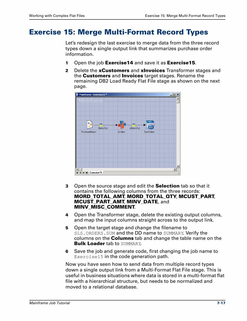
Working with Complex Flat Files Exercise 15: Merge Multi-Format Record Types
Exercise 15: Merge Multi-Format Record TypesLet’s redesign the last exercise to merge data from the three record
types down a single output link that summarizes purchase order
information.
1 Open the job Exercise14 and save it as Exercise15.
2 Delete the xCustomers and xInvoices Transformer stages and the Customers and Invoices target stages. Rename the remaining DB2 Load Ready Flat File stage as shown on the next page.
3 Open the source stage and edit the Selection tab so that it contains the following columns from the three records: MORD_TOTAL_AMT, MORD_TOTAL_QTY, MCUST_PART, MCUST_PART_AMT, MINV_DATE, and MINV_MISC_COMMENT.
4 Open the Transformer stage, delete the existing output columns, and map the input columns straight across to the output link.
5 Open the target stage and change the filename to SLS.ORDERS.SUM and the DD name to SUMMARY. Verify the columns on the Columns tab and change the table name on the Bulk Loader tab to SUMMARY.
6 Save the job and generate code, first changing the job name to Exercise15 in the code generation path.
Now you have seen how to send data from multiple record types
down a single output link from a Multi-Format Flat File stage. This is
useful in business situations where data is stored in a multi-format flat
file with a hierarchical structure, but needs to be normalized and
moved to a relational database.
Mainframe Job Tutorial 7-17
Summary Working with Complex Flat Files
SummaryIn this chapter you created jobs to work with different types of flat file
data. You read data from both complex and multi-format flat files and
learned how to normalize and flatten arrays. You wrote data to
delimited and DB2 load ready flat files and specified the target file
parameters. The exercises in this chapter gave you a chance to test
what you’ve learned about importing meta data, configuring stages,
defining constraints and stage variables, and specifying job
parameters.
7-18 Mainframe Job Tutorial
8Working with IMS Data
This chapter introduces you to the IMS stage in mainframe jobs. IMS
stages are used to read data from databases in IMS version 5 and
above. When you use an IMS stage, you can view the segment
hierarchy of an IMS database and select a path of segments to output
data from. You can choose to perform either partial path or complete
path processing. You can also add an end-of-data indicator, normalize
or flatten arrays, and define a constraint to limit output data.
The exercises in this chapter show you how to import meta data from
IMS definitions and configure the IMS stage as a source in a job. In
Exercise 16 you import meta data from an IMS Data Base Description
(DBD) file and an IMS Program Specification Block (PSB) file. You
become familiar with the structure of the imported meta data by
viewing the details of the data using Ascential DataStage’s IMS DBD
Editor and IMS Viewset Editor.
In Exercise 17 you create a job that provides information about
inventory for an auto dealership. It reads data from an IMS source,
transforms it, and writes it to a flat file target. You see how to select an
IMS segment path and output columns, and you define a constraint to
limit output data.
Exercise 16: Import IMS DefinitionsYou can import IMS definitions into the Repository from DBD files and
PSB files. A DBD defines the structure of an IMS database. A PSB
defines an application’s view of an IMS database. You must import a
DBD before you import its associated PSBs.
Mainframe Job Tutorial 8-1
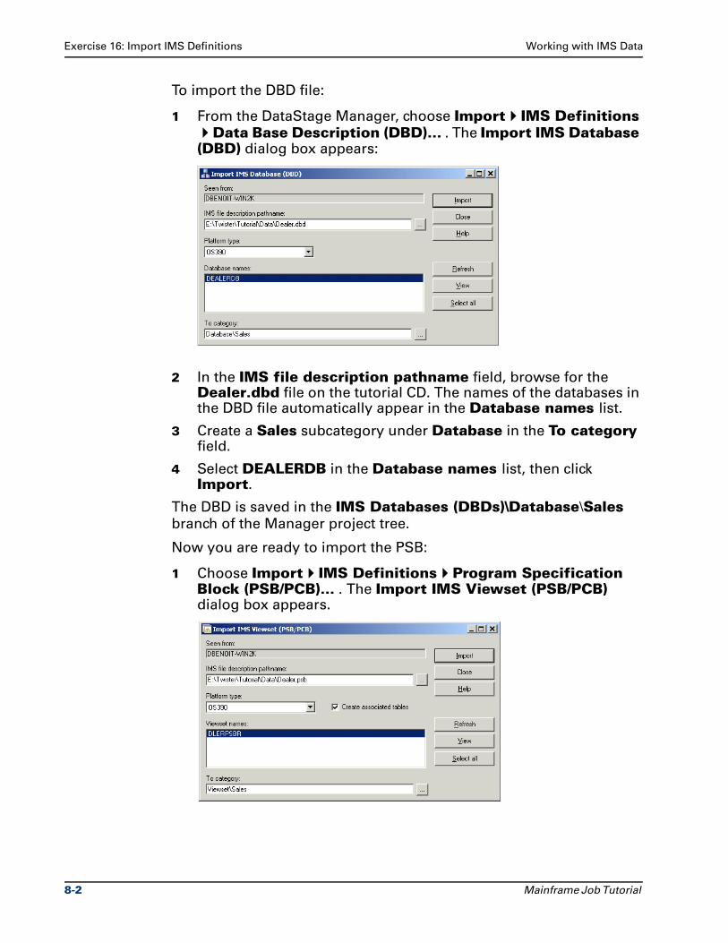
Exercise 16: Import IMS Definitions Working with IMS Data
To import the DBD file:
1 From the DataStage Manager, choose Import IMS Definitions
Data Base Description (DBD)… . The Import IMS Database (DBD) dialog box appears:
2 In the IMS file description pathname field, browse for the Dealer.dbd file on the tutorial CD. The names of the databases in the DBD file automatically appear in the Database names list.
3 Create a Sales subcategory under Database in the To category field.
4 Select DEALERDB in the Database names list, then click Import.
The DBD is saved in the IMS Databases (DBDs)\Database\Sales
branch of the Manager project tree.
Now you are ready to import the PSB:
1 Choose Import IMS Definitions Program Specification Block (PSB/PCB)… . The Import IMS Viewset (PSB/PCB) dialog box appears.
8-2 Mainframe Job Tutorial
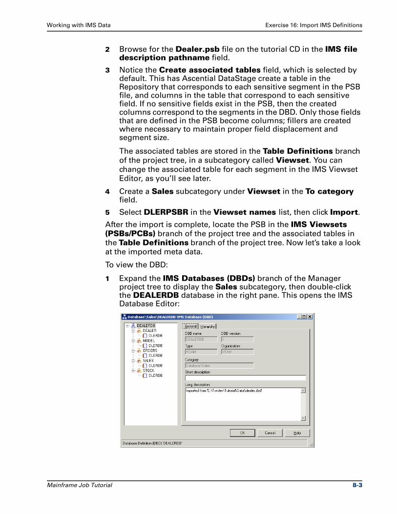
Working with IMS Data Exercise 16: Import IMS Definitions
2 Browse for the Dealer.psb file on the tutorial CD in the IMS file description pathname field.
3 Notice the Create associated tables field, which is selected by default. This has Ascential DataStage create a table in the Repository that corresponds to each sensitive segment in the PSB file, and columns in the table that correspond to each sensitive field. If no sensitive fields exist in the PSB, then the created columns correspond to the segments in the DBD. Only those fields that are defined in the PSB become columns; fillers are created where necessary to maintain proper field displacement and segment size.
The associated tables are stored in the Table Definitions branch
of the project tree, in a subcategory called Viewset. You can
change the associated table for each segment in the IMS Viewset
Editor, as you’ll see later.
4 Create a Sales subcategory under Viewset in the To category field.
5 Select DLERPSBR in the Viewset names list, then click Import.
After the import is complete, locate the PSB in the IMS Viewsets (PSBs/PCBs) branch of the project tree and the associated tables in
the Table Definitions branch of the project tree. Now let’s take a look
at the imported meta data.
To view the DBD:
1 Expand the IMS Databases (DBDs) branch of the Manager project tree to display the Sales subcategory, then double-click the DEALERDB database in the right pane. This opens the IMS Database Editor:
Mainframe Job Tutorial 8-3
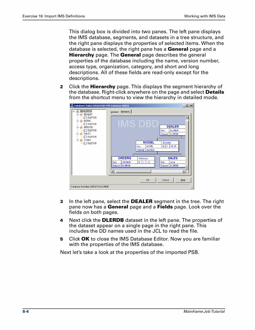
Exercise 16: Import IMS Definitions Working with IMS Data
This dialog box is divided into two panes. The left pane displays
the IMS database, segments, and datasets in a tree structure, and
the right pane displays the properties of selected items. When the
database is selected, the right pane has a General page and a
Hierarchy page. The General page describes the general
properties of the database including the name, version number,
access type, organization, category, and short and long
descriptions. All of these fields are read-only except for the
descriptions.
2 Click the Hierarchy page. This displays the segment hierarchy of the database. Right-click anywhere on the page and select Details from the shortcut menu to view the hierarchy in detailed mode.
3 In the left pane, select the DEALER segment in the tree. The right pane now has a General page and a Fields page. Look over the fields on both pages.
4 Next click the DLERDB dataset in the left pane. The properties of the dataset appear on a single page in the right pane. This includes the DD names used in the JCL to read the file.
5 Click OK to close the IMS Database Editor. Now you are familiar with the properties of the IMS database.
Next let’s take a look at the properties of the imported PSB.
8-4 Mainframe Job Tutorial
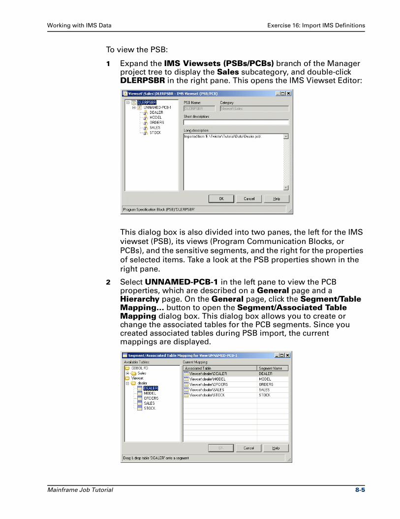
Working with IMS Data Exercise 16: Import IMS Definitions
To view the PSB:
1 Expand the IMS Viewsets (PSBs/PCBs) branch of the Manager project tree to display the Sales subcategory, and double-click DLERPSBR in the right pane. This opens the IMS Viewset Editor:
This dialog box is also divided into two panes, the left for the IMS
viewset (PSB), its views (Program Communication Blocks, or
PCBs), and the sensitive segments, and the right for the properties
of selected items. Take a look at the PSB properties shown in the
right pane.
2 Select UNNAMED-PCB-1 in the left pane to view the PCB properties, which are described on a General page and a Hierarchy page. On the General page, click the Segment/Table Mapping… button to open the Segment/Associated Table Mapping dialog box. This dialog box allows you to create or change the associated tables for the PCB segments. Since you created associated tables during PSB import, the current mappings are displayed.
Mainframe Job Tutorial 8-5
Exercise 17: Read Data from an IMS Source Working with IMS Data
The left pane displays available tables in the Repository which are
of type QSAM_SEQ_COMPLEX. The right pane displays the
segment names and the tables currently associated with them.
You can clear one or all of the current table mappings using the
right mouse button. To change the table association for a
segment, select a table in the left pane and drag it to the segment
in the right pane. When you are finished, click OK. In this case,
keep the current mappings and click Cancel to return to the IMS
Viewset Editor.
3 Click the Hierarchy page and view the PCB segment hierarchy in detailed mode.
4 Select one of the sensitive segments in the left pane, such as DEALER. Its properties are displayed on a General page, a Sen Fields page, and a Columns page. Notice the browse button next to the Associate table field on the General page; clicking this lets you change the table associated with a particular segment if desired.
5 Click OK to close the IMS Viewset Editor.
You have now defined the meta data for your IMS source and viewed
its properties.
Exercise 17: Read Data from an IMS SourceIn this exercise you design a job that reads data from an IMS source
with information about auto dealers. The job determines the available
stock of cars priced under $25,000. You see how to select the PSB and
its associated PCB that define the view of the IMS database. You also
see how to select the segment path to output data from the stage. You
then pass the data through a Transformer stage and write it out to a
flat file target.
To design the job:
1 Create a new mainframe job and save it as Exercise17.
2 From left to right, add an IMS stage, a Transformer stage, and a Fixed-Width Flat File stage. Link the stages together and rename the stages and links as shown on the next page.
8-6 Mainframe Job Tutorial
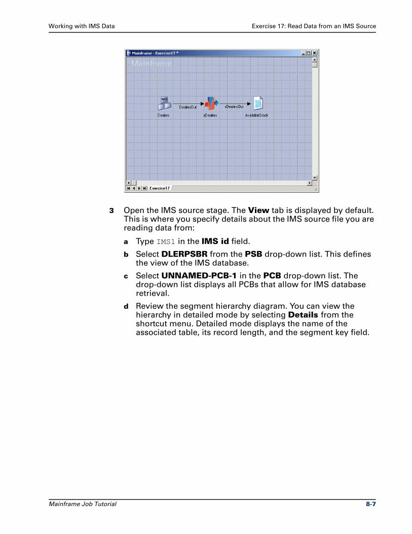
Working with IMS Data Exercise 17: Read Data from an IMS Source
3 Open the IMS source stage. The View tab is displayed by default. This is where you specify details about the IMS source file you are reading data from:
a Type IMS1 in the IMS id field.
b Select DLERPSBR from the PSB drop-down list. This defines the view of the IMS database.
c Select UNNAMED-PCB-1 in the PCB drop-down list. The drop-down list displays all PCBs that allow for IMS database retrieval.
d Review the segment hierarchy diagram. You can view the hierarchy in detailed mode by selecting Details from the shortcut menu. Detailed mode displays the name of the associated table, its record length, and the segment key field.
Mainframe Job Tutorial 8-7
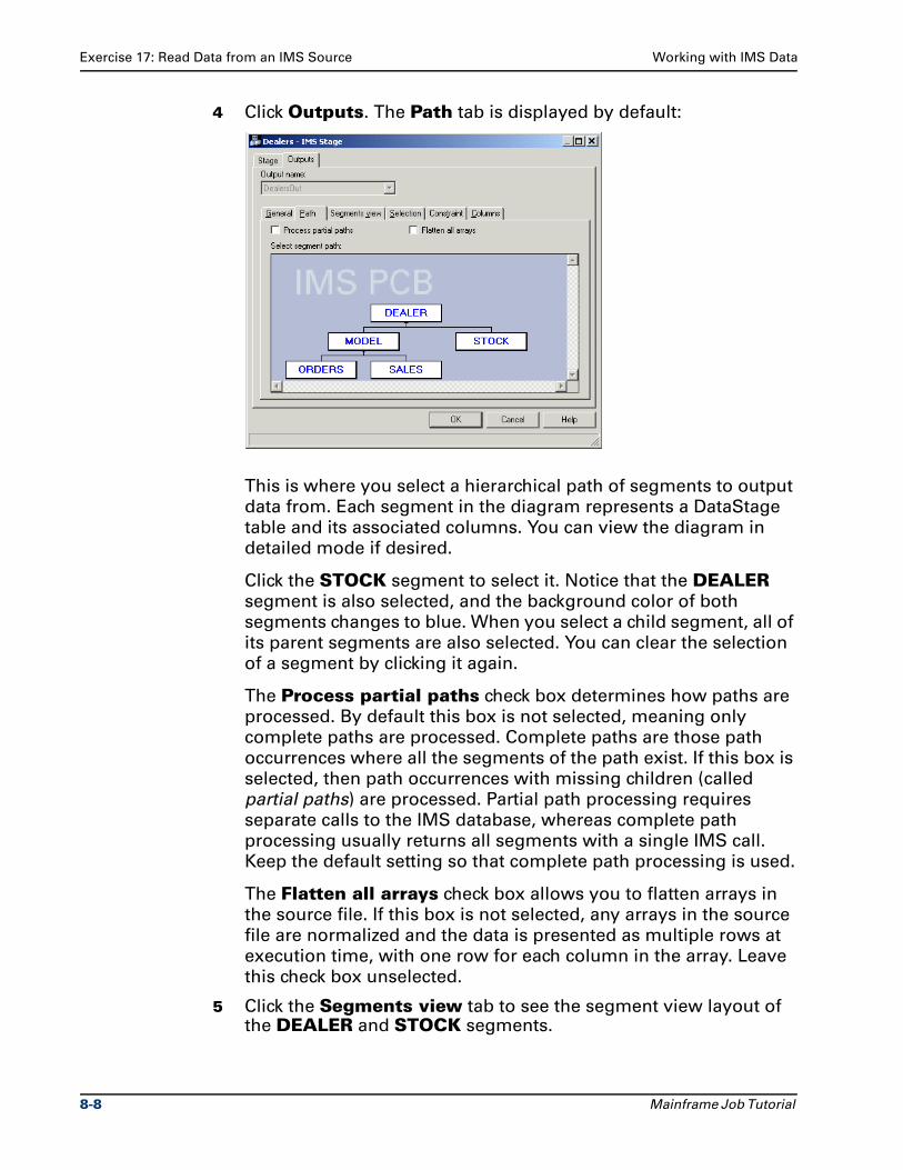
Exercise 17: Read Data from an IMS Source Working with IMS Data
4 Click Outputs. The Path tab is displayed by default:
This is where you select a hierarchical path of segments to output
data from. Each segment in the diagram represents a DataStage
table and its associated columns. You can view the diagram in
detailed mode if desired.
Click the STOCK segment to select it. Notice that the DEALER
segment is also selected, and the background color of both
segments changes to blue. When you select a child segment, all of
its parent segments are also selected. You can clear the selection
of a segment by clicking it again.
The Process partial paths check box determines how paths are
processed. By default this box is not selected, meaning only
complete paths are processed. Complete paths are those path
occurrences where all the segments of the path exist. If this box is
selected, then path occurrences with missing children (called
partial paths) are processed. Partial path processing requires
separate calls to the IMS database, whereas complete path
processing usually returns all segments with a single IMS call.
Keep the default setting so that complete path processing is used.
The Flatten all arrays check box allows you to flatten arrays in
the source file. If this box is not selected, any arrays in the source
file are normalized and the data is presented as multiple rows at
execution time, with one row for each column in the array. Leave
this check box unselected.
5 Click the Segments view tab to see the segment view layout of the DEALER and STOCK segments.
8-8 Mainframe Job Tutorial
Working with IMS Data Summary
6 Click the Selection tab and move everything except the two filler columns to the Selected columns list.
7 On the Constraint tab, define a constraint that selects all vehicles with a price less than $25,000.00.
8 Click OK to accept the settings. The IMS source stage is now complete.
9 Propagate the input columns to the output link in the Transformer stage.
10 Configure the target Fixed-Width Flat File stage to write data to a new file named INSTOCK.
11 Save the job and generate code. In the Code generation dialog box, notice the IMS Program Type field. This specifies the type of IMS program being read by the job. Keep the default setting of DLI.
You have now read data from an IMS source. You specified the
segment path for reading data and selected the columns to be output
from the stage.
SummaryIn this chapter you learned how to import data from IMS sources and
use an IMS stage in a job. You viewed the details of the imported meta
data, including the segment hierarchy, and saw how table
associations for each segment are created in the Manager. You then
configured the IMS stage as a source in a job that determined the
available stock of cars priced under $25,000 from auto dealerships.
You selected the segment path to read data from, and defined a
constraint to limit the output data.
Next you learn how to work with Relational stages.
Mainframe Job Tutorial 8-9
9Working with Relational Data
This chapter introduces you to the Relational stage in mainframe jobs.
Relational stages are used to read data from or write data to DB2
tables on OS/390 platforms.
In Exercise 18 you create a job using a Relational source stage and a
Fixed-Width Flat File target stage. You define a computed column that
is the concatenation of two input columns. Then you build a WHERE
clause to join data from two DB2 tables and specify selection criteria
for writing data to the output link.
In Exercise 19 you create a job that consists of both a Relational
source stage and a Relational target stage. You define the target stage
so that it updates existing records or inserts new records in the table.
Relational StagesRelational stages extract data from and write data to tables in DB2
UDB 5.1 and later. When used as a source, Relational stages have
separate tabs for defining a SQL SELECT statement. You identify the
source table, select columns to be output from the stage, and define
the conditions needed to build WHERE, GROUP BY, HAVING, and
ORDER BY clauses. You can also type your own SQL statement if you
need to perform complex joins or subselects. An integrated parser
validates your syntax against SQL-92 standards.
When used as a target, Relational stages provide a variety of options
for writing data to an existing DB2 table. You can choose to insert new
rows, update existing rows, replace existing rows, or delete rows,
depending on your requirements. You identify the table to write data
to, select the update action and the columns to update, and specify
the update condition.
Mainframe Job Tutorial 9-1
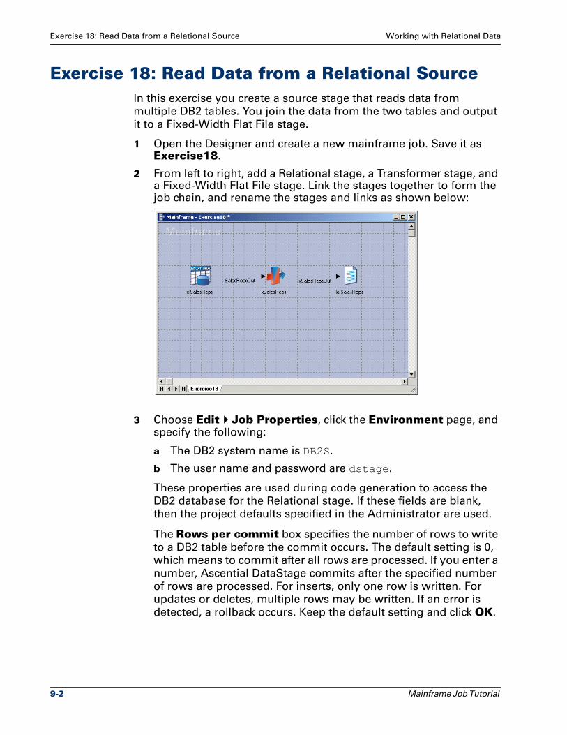
Exercise 18: Read Data from a Relational Source Working with Relational Data
Exercise 18: Read Data from a Relational SourceIn this exercise you create a source stage that reads data from
multiple DB2 tables. You join the data from the two tables and output
it to a Fixed-Width Flat File stage.
1 Open the Designer and create a new mainframe job. Save it as Exercise18.
2 From left to right, add a Relational stage, a Transformer stage, and a Fixed-Width Flat File stage. Link the stages together to form the job chain, and rename the stages and links as shown below:
3 Choose Edit Job Properties, click the Environment page, and specify the following:
a The DB2 system name is DB2S.
b The user name and password are dstage.
These properties are used during code generation to access the
DB2 database for the Relational stage. If these fields are blank,
then the project defaults specified in the Administrator are used.
The Rows per commit box specifies the number of rows to write
to a DB2 table before the commit occurs. The default setting is 0,
which means to commit after all rows are processed. If you enter a
number, Ascential DataStage commits after the specified number
of rows are processed. For inserts, only one row is written. For
updates or deletes, multiple rows may be written. If an error is
detected, a rollback occurs. Keep the default setting and click OK.
9-2 Mainframe Job Tutorial
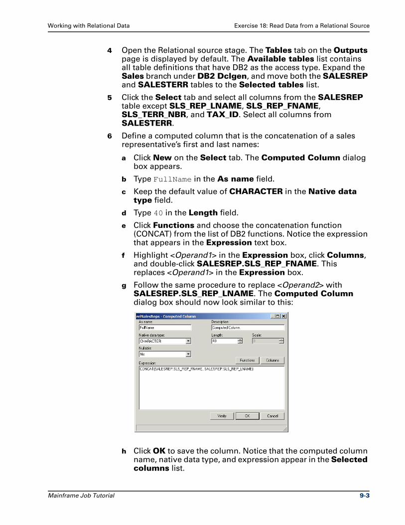
Working with Relational Data Exercise 18: Read Data from a Relational Source
4 Open the Relational source stage. The Tables tab on the Outputs page is displayed by default. The Available tables list contains all table definitions that have DB2 as the access type. Expand the Sales branch under DB2 Dclgen, and move both the SALESREP and SALESTERR tables to the Selected tables list.
5 Click the Select tab and select all columns from the SALESREP table except SLS_REP_LNAME, SLS_REP_FNAME, SLS_TERR_NBR, and TAX_ID. Select all columns from SALESTERR.
6 Define a computed column that is the concatenation of a sales representative’s first and last names:
a Click New on the Select tab. The Computed Column dialog box appears.
b Type FullName in the As name field.
c Keep the default value of CHARACTER in the Native data type field.
d Type 40 in the Length field.
e Click Functions and choose the concatenation function (CONCAT) from the list of DB2 functions. Notice the expression that appears in the Expression text box.
f Highlight <Operand1> in the Expression box, click Columns, and double-click SALESREP.SLS_REP_FNAME. This replaces <Operand1> in the Expression box.
g Follow the same procedure to replace <Operand2> with SALESREP.SLS_REP_LNAME. The Computed Column dialog box should now look similar to this:
h Click OK to save the column. Notice that the computed column name, native data type, and expression appear in the Selected columns list.
Mainframe Job Tutorial 9-3
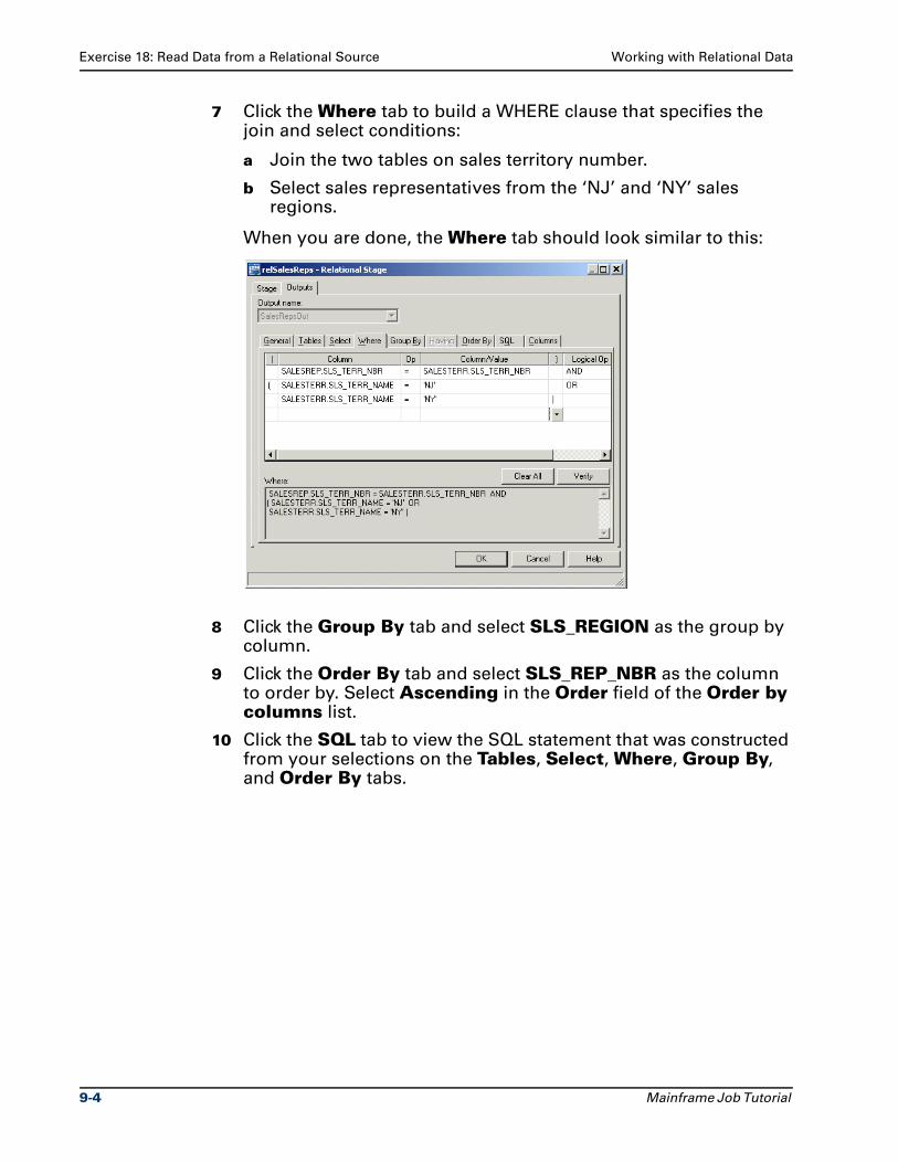
Exercise 18: Read Data from a Relational Source Working with Relational Data
7 Click the Where tab to build a WHERE clause that specifies the join and select conditions:
a Join the two tables on sales territory number.
b Select sales representatives from the ‘NJ’ and ‘NY’ sales regions.
When you are done, the Where tab should look similar to this:
8 Click the Group By tab and select SLS_REGION as the group by column.
9 Click the Order By tab and select SLS_REP_NBR as the column to order by. Select Ascending in the Order field of the Order by columns list.
10 Click the SQL tab to view the SQL statement that was constructed from your selections on the Tables, Select, Where, Group By, and Order By tabs.
9-4 Mainframe Job Tutorial
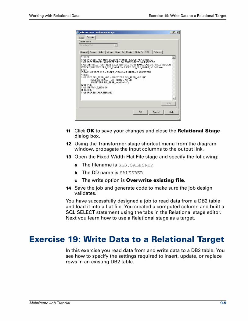
Working with Relational Data Exercise 19: Write Data to a Relational Target
11 Click OK to save your changes and close the Relational Stage dialog box.
12 Using the Transformer stage shortcut menu from the diagram window, propagate the input columns to the output link.
13 Open the Fixed-Width Flat File stage and specify the following:
a The filename is SLS.SALESREP.
b The DD name is SALESREP.
c The write option is Overwrite existing file.
14 Save the job and generate code to make sure the job design validates.
You have successfully designed a job to read data from a DB2 table
and load it into a flat file. You created a computed column and built a
SQL SELECT statement using the tabs in the Relational stage editor.
Next you learn how to use a Relational stage as a target.
Exercise 19: Write Data to a Relational TargetIn this exercise you read data from and write data to a DB2 table. You
see how to specify the settings required to insert, update, or replace
rows in an existing DB2 table.
Mainframe Job Tutorial 9-5
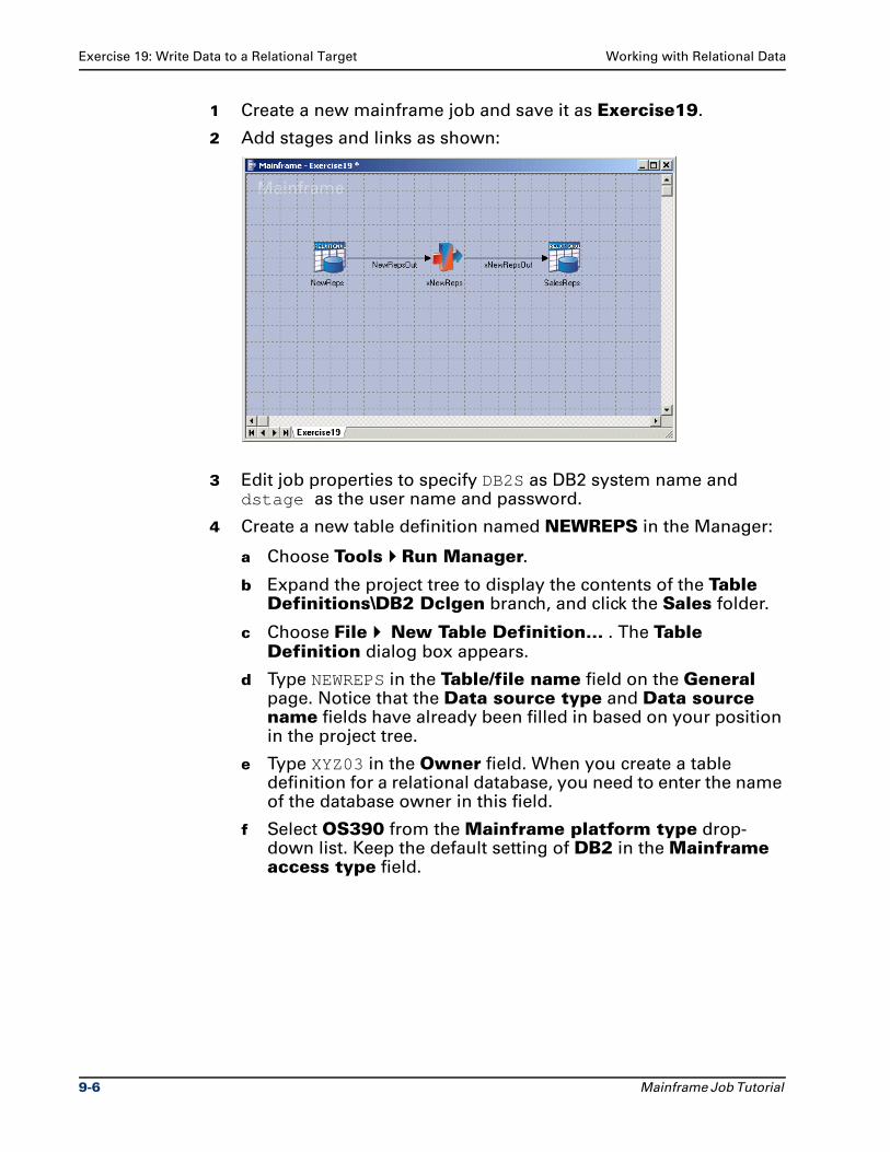
Exercise 19: Write Data to a Relational Target Working with Relational Data
1 Create a new mainframe job and save it as Exercise19.
2 Add stages and links as shown:
3 Edit job properties to specify DB2S as DB2 system name and dstage as the user name and password.
4 Create a new table definition named NEWREPS in the Manager:
a Choose Tools Run Manager.
b Expand the project tree to display the contents of the Table Definitions\DB2 Dclgen branch, and click the Sales folder.
c Choose File New Table Definition… . The Table Definition dialog box appears.
d Type NEWREPS in the Table/file name field on the General page. Notice that the Data source type and Data source name fields have already been filled in based on your position in the project tree.
e Type XYZ03 in the Owner field. When you create a table definition for a relational database, you need to enter the name of the database owner in this field.
f Select OS390 from the Mainframe platform type drop-down list. Keep the default setting of DB2 in the Mainframe access type field.
9-6 Mainframe Job Tutorial
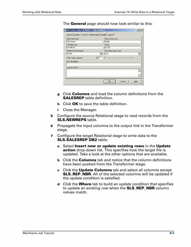
Working with Relational Data Exercise 19: Write Data to a Relational Target
The General page should now look similar to this:
g Click Columns and load the column definitions from the SALESREP table definition.
h Click OK to save the table definition.
i Close the Manager.
5 Configure the source Relational stage to read records from the SLS.NEWREPS table.
6 Propagate the input columns to the output link in the Transformer stage.
7 Configure the target Relational stage to write data to the SLS.SALESREP DB2 table:
a Select Insert new or update existing rows in the Update action drop-down list. This specifies how the target file is updated. Take a look at the other options that are available.
b Click the Columns tab and notice that the column definitions have been pushed from the Transformer stage.
c Click the Update Columns tab and select all columns except SLS_REP_NBR. All of the selected columns will be updated if the update condition is satisfied.
d Click the Where tab to build an update condition that specifies to update an existing row when the SLS_REP_NBR column values match.
Mainframe Job Tutorial 9-7
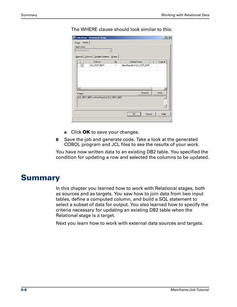
Summary Working with Relational Data
The WHERE clause should look similar to this:
e Click OK to save your changes.
8 Save the job and generate code. Take a look at the generated COBOL program and JCL files to see the results of your work.
You have now written data to an existing DB2 table. You specified the
condition for updating a row and selected the columns to be updated.
SummaryIn this chapter you learned how to work with Relational stages, both
as sources and as targets. You saw how to join data from two input
tables, define a computed column, and build a SQL statement to
select a subset of data for output. You also learned how to specify the
criteria necessary for updating an existing DB2 table when the
Relational stage is a target.
Next you learn how to work with external data sources and targets.
9-8 Mainframe Job Tutorial
10Working with External
Sources and Targets
You have seen how to work with a variety of flat files and relational
databases in DataStage mainframe jobs. This chapter shows you how
to work with external data sources and targets. These are file types
that do not have built-in support within Ascential DataStage
Enterprise MVS Edition.
Before you design a job using an external source or target, you must
first write a program outside of Ascential DataStage that reads data
from the external source or writes data to the external target. You can
write the program in any language that is callable from COBOL.
Ascential DataStage calls your program from its generated COBOL
program. The call interface between the two programs consists of two
parameters:
The address of the control structure
The address of the record definition
For information on defining the call interface, see Ascential DataStage
Mainframe Job Developer’s Guide.
After you write the external program, you create a routine definition in
the DataStage Manager. The routine specifies the attributes of the
external program, including the library path, invocation method and
routine arguments, so that it can be called by Ascential DataStage.
The last step is to design the job, using an External Source stage or an
External Target stage to represent the external program.
In Exercise 20 you learn how to define and call an external source
program in a mainframe job. You create an external source routine in
the Manager and design a job using an External Source stage. You
Mainframe Job Tutorial 10-1
Exercise 20: Read Data From an External Source Working with External Sources and Targets
also practice saving output columns as a table definition in the
Repository.
In Exercise 21 you follow a similar procedure to create an external
target routine in the Manager and design a job using an External
Target stage.
Exercise 20: Read Data From an External SourceLet’s assume you have written a program to retrieve purchase order
data from an external data source. Now you create an external source
routine in the DataStage Manager and design a job that calls it. You
also save the output columns as a table definition in the Repository,
making it available to load into other stages in your job design.
Define External Source Routine Meta DataThe first step is to import the table definition and define routine meta
data for the external source program. These actions can be performed
either in the DataStage Manager or the Repository window of the
DataStage Designer:
1 Right-click the Table Definitions branch of the project tree and choose Import COBOL File Definitions…. Import the EXT_ORDERS table definition from the External.cfd file. Save the table in a new category named COBOL FD\External.
2 Right-click the Routines branch of the project tree and choose New Mainframe Routine… to open the Mainframe Routine dialog box. Specify the basic characteristics of the routine on the General page:
a Type PURCHORD in the Routine name field. Notice that this name also appears in the External subroutine name field. This is because the two names must match if the invocation method is dynamic (the default).
The routine name is the name the routine is known by in
Ascential DataStage, while the external subroutine name is the
actual name of the external routine. If the invocation method is
static, these two names can be different because the names
can be resolved when the program is link edited.
b Select External Source Routine in the Type field.
c Type External\Sales in the Category field.
d Click Static in the Invocation method area.
10-2 Mainframe Job Tutorial
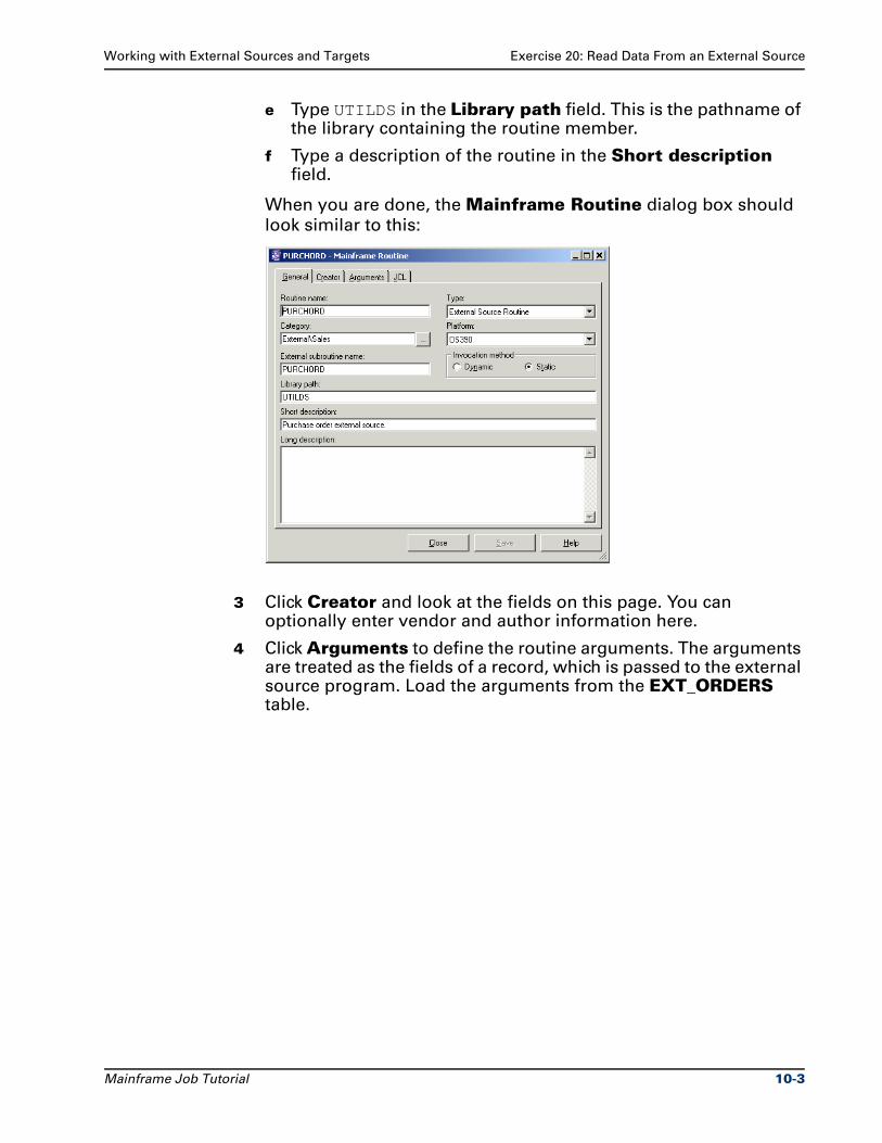
Working with External Sources and Targets Exercise 20: Read Data From an External Source
e Type UTILDS in the Library path field. This is the pathname of the library containing the routine member.
f Type a description of the routine in the Short description field.
When you are done, the Mainframe Routine dialog box should
look similar to this:
3 Click Creator and look at the fields on this page. You can optionally enter vendor and author information here.
4 Click Arguments to define the routine arguments. The arguments are treated as the fields of a record, which is passed to the external source program. Load the arguments from the EXT_ORDERS table.
Mainframe Job Tutorial 10-3
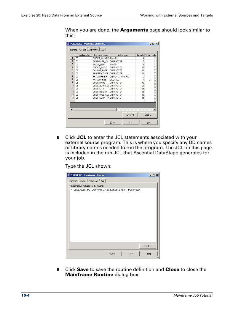
Exercise 20: Read Data From an External Source Working with External Sources and Targets
When you are done, the Arguments page should look similar to
this:
5 Click JCL to enter the JCL statements associated with your external source program. This is where you specify any DD names or library names needed to run the program. The JCL on this page is included in the run JCL that Ascential DataStage generates for your job.
Type the JCL shown:
6 Click Save to save the routine definition and Close to close the Mainframe Routine dialog box.
10-4 Mainframe Job Tutorial
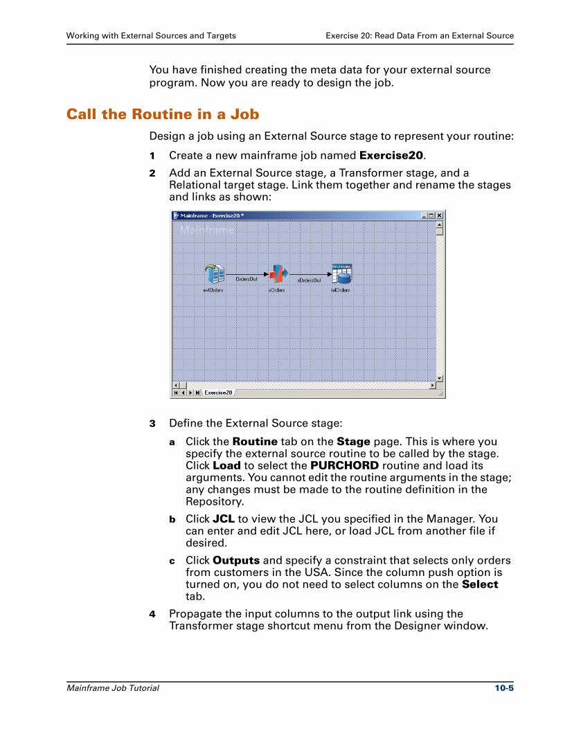
Working with External Sources and Targets Exercise 20: Read Data From an External Source
You have finished creating the meta data for your external source
program. Now you are ready to design the job.
Call the Routine in a JobDesign a job using an External Source stage to represent your routine:
1 Create a new mainframe job named Exercise20.
2 Add an External Source stage, a Transformer stage, and a Relational target stage. Link them together and rename the stages and links as shown:
3 Define the External Source stage:
a Click the Routine tab on the Stage page. This is where you specify the external source routine to be called by the stage. Click Load to select the PURCHORD routine and load its arguments. You cannot edit the routine arguments in the stage; any changes must be made to the routine definition in the Repository.
b Click JCL to view the JCL you specified in the Manager. You can enter and edit JCL here, or load JCL from another file if desired.
c Click Outputs and specify a constraint that selects only orders from customers in the USA. Since the column push option is turned on, you do not need to select columns on the Select tab.
4 Propagate the input columns to the output link using the Transformer stage shortcut menu from the Designer window.
Mainframe Job Tutorial 10-5
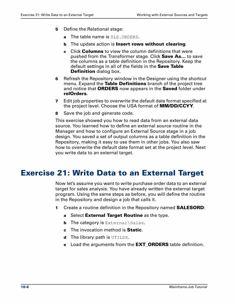
Exercise 21: Write Data to an External Target Working with External Sources and Targets
5 Define the Relational stage:
a The table name is SLS.ORDERS.
b The update action is Insert rows without clearing.
c Click Columns to view the column definitions that were pushed from the Transformer stage. Click Save As… to save the columns as a table definition in the Repository. Keep the default settings in all of the fields in the Save Table Definition dialog box.
6 Refresh the Repository window in the Designer using the shortcut menu. Expand the Table Definitions branch of the project tree and notice that ORDERS now appears in the Saved folder under relOrders.
7 Edit job properties to overwrite the default date format specified at the project level. Choose the USA format of MM/DD/CCYY.
8 Save the job and generate code.
This exercise showed you how to read data from an external data
source. You learned how to define an external source routine in the
Manager and how to configure an External Source stage in a job
design. You saved a set of output columns as a table definition in the
Repository, making it easy to use them in other jobs. You also saw
how to overwrite the default date format set at the project level. Next
you write data to an external target.
Exercise 21: Write Data to an External TargetNow let’s assume you want to write purchase order data to an external
target for sales analysis. You have already written the external target
program. Using the same steps as before, you will define the routine
in the Repository and design a job that calls it.
1 Create a routine definition in the Repository named SALESORD:
a Select External Target Routine as the type.
b The category is External\Sales.
c The invocation method is Static.
d The library path is UTILDS.
e Load the arguments from the EXT_ORDERS table definition.
10-6 Mainframe Job Tutorial
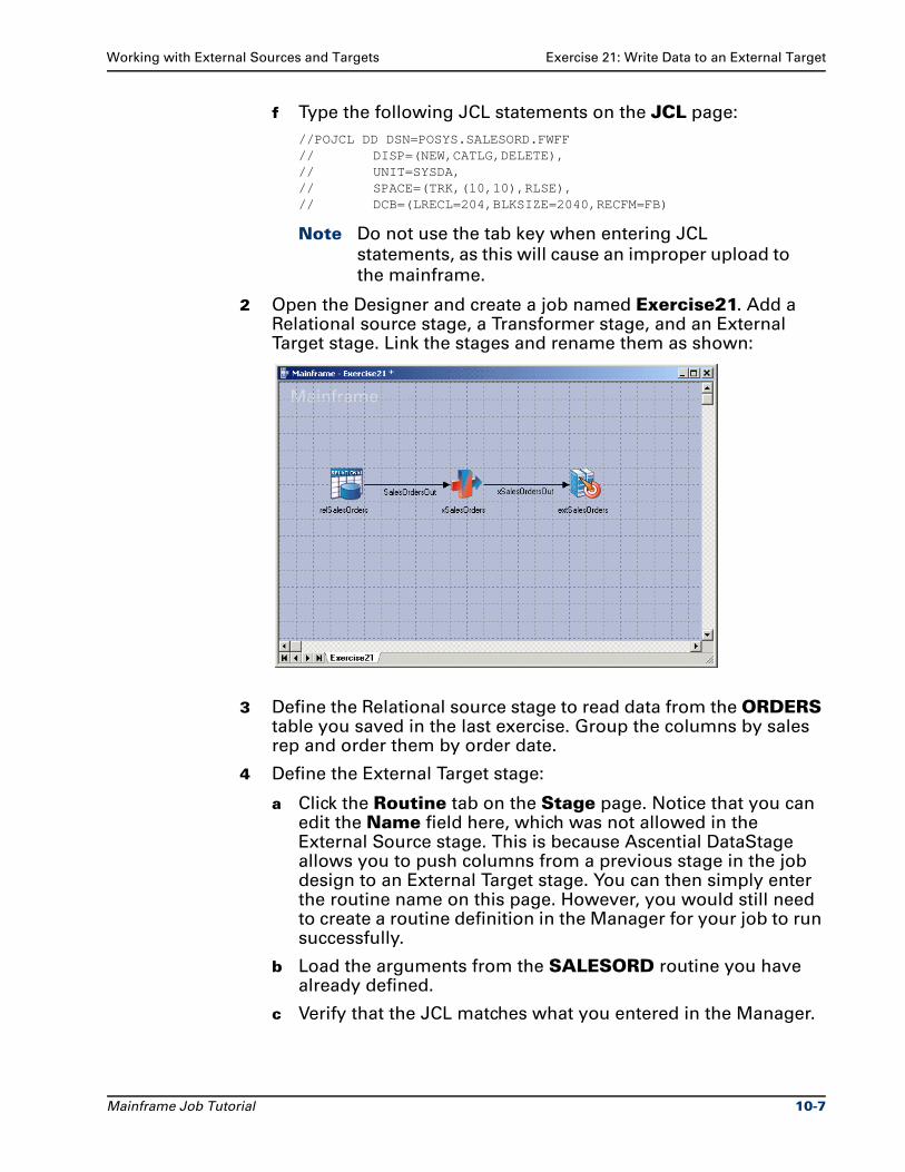
Working with External Sources and Targets Exercise 21: Write Data to an External Target
f Type the following JCL statements on the JCL page:
//POJCL DD DSN=POSYS.SALESORD.FWFF// DISP=(NEW,CATLG,DELETE),// UNIT=SYSDA,// SPACE=(TRK,(10,10),RLSE),// DCB=(LRECL=204,BLKSIZE=2040,RECFM=FB)
Note Do not use the tab key when entering JCL
statements, as this will cause an improper upload to
the mainframe.
2 Open the Designer and create a job named Exercise21. Add a Relational source stage, a Transformer stage, and an External Target stage. Link the stages and rename them as shown:
3 Define the Relational source stage to read data from the ORDERS table you saved in the last exercise. Group the columns by sales rep and order them by order date.
4 Define the External Target stage:
a Click the Routine tab on the Stage page. Notice that you can edit the Name field here, which was not allowed in the External Source stage. This is because Ascential DataStage allows you to push columns from a previous stage in the job design to an External Target stage. You can then simply enter the routine name on this page. However, you would still need to create a routine definition in the Manager for your job to run successfully.
b Load the arguments from the SALESORD routine you have already defined.
c Verify that the JCL matches what you entered in the Manager.
Mainframe Job Tutorial 10-7
Summary Working with External Sources and Targets
5 Open the Transformer stage and use column auto-match to define the column mappings.
6 Save the job and generate code.
You have successfully designed a job that writes data to an external
target. Now your business analysts can review the sales orders placed
by each sales representative, working from their own familiar
platform.
SummaryThis chapter showed you how to work with external sources and
targets in mainframe jobs. You learned how to create a routine
definition for your external source and target programs. You designed
one job that read external purchase order data from an external
source, and another job that wrote sales order information to an
external target for analysis.
You are now familiar with all of the passive stages in mainframe jobs,
including those that provide built-in support for various file types and
those that allow you to work with external sources and targets. Next,
you start working with the active stages. You’ll see the powerful
options Ascential DataStage provides for manipulating data so that it
is efficiently organized in the data warehouse.
10-8 Mainframe Job Tutorial
11Merging Data Using Joins
and Lookups
Now that you understand how to work with data sources and targets
in mainframe jobs, you are ready to use active stages to process the
data being moved into a data warehouse. This chapter introduces you
to Join and Lookup stages.
Join stages are used to join data from two sources. You can use the
Join stage to perform inner joins, outer joins, or full joins:
Inner joins return only the matching rows from both input tables.
Outer joins return all rows from the outer table (you designate one of the inputs as the outer link) even if no matches are found.
Full joins return all rows that match the join condition, plus the unmatched rows from both input tables.
Lookup stages are used to look up reference information. There are
two lookup types:
A singleton lookup returns a single matching row
A cursor lookup returns all matching rows
You can also perform conditional lookups, which are based on a pre-
lookup condition that must be met before the lookup occurs.
In Exercise 22 you join two data sources. You specify the join type and
the join technique, you define the join condition, and then you map
the joined data to your output link.
In Exercise 23 you look up information from a reference table. You
specify the lookup technique and the action to take if the lookup fails.
You then define the lookup condition and the output column
Mainframe Job Tutorial 11-1
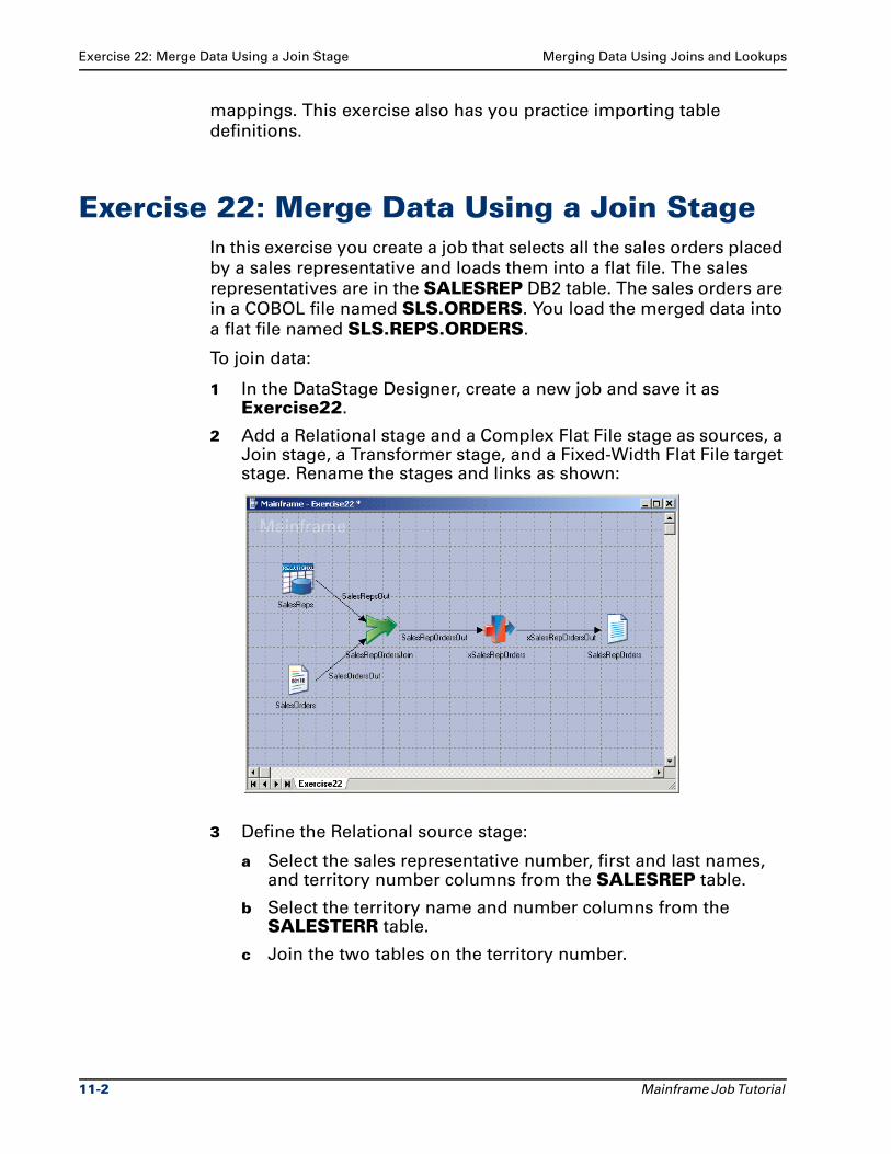
Exercise 22: Merge Data Using a Join Stage Merging Data Using Joins and Lookups
mappings. This exercise also has you practice importing table
definitions.
Exercise 22: Merge Data Using a Join StageIn this exercise you create a job that selects all the sales orders placed
by a sales representative and loads them into a flat file. The sales
representatives are in the SALESREP DB2 table. The sales orders are
in a COBOL file named SLS.ORDERS. You load the merged data into
a flat file named SLS.REPS.ORDERS.
To join data:
1 In the DataStage Designer, create a new job and save it as Exercise22.
2 Add a Relational stage and a Complex Flat File stage as sources, a Join stage, a Transformer stage, and a Fixed-Width Flat File target stage. Rename the stages and links as shown:
3 Define the Relational source stage:
a Select the sales representative number, first and last names, and territory number columns from the SALESREP table.
b Select the territory name and number columns from the SALESTERR table.
c Join the two tables on the territory number.
11-2 Mainframe Job Tutorial
Merging Data Using Joins and Lookups Exercise 22: Merge Data Using a Join Stage
4 Define the Complex Flat File source stage:
a Read data from the SLS.ORDERS file.
b Load the columns from the SALES_ORDERS table definition. There are no arrays in this table, so the Complex file load option dialog box does not appear.
5 Define the Join stage to merge the data coming from the SalesReps and SalesOrders stages:
a Click Inner join in the Join type area.
b Select SalesOrdersOut as the outer link.
c Look at the options in the Join technique drop-down list:
– Auto lets Ascential DataStage choose the best technique based on the information you specify in the stage.
– Hash builds an in-memory hash table on the inner link.
– Nested scans each row of the inner table for matching values.
– Two File Match scans both input tables (which must be presorted on the matching keys) at once to determine if there are matching values.
Accept the default setting of Auto.
d Click the Inputs page and view the column definitions for the two input links. Select each link from the Input name drop-down list. Input column definitions are read-only in all of the active stages.
e Click the Outputs page. The Join Condition tab is displayed by default. This is where you specify the condition for merging data from the two tables. Build an expression that merges the two files based on finding matching sales representative numbers, as shown on the next page.
Mainframe Job Tutorial 11-3
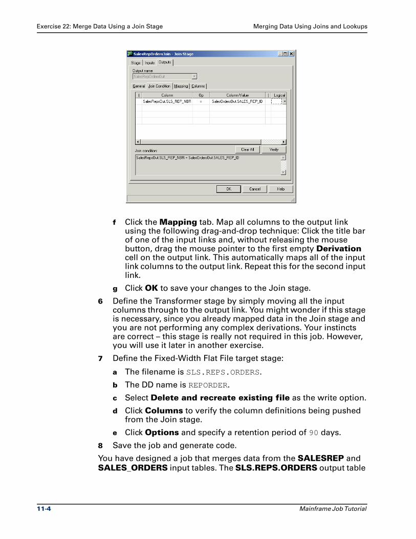
Exercise 22: Merge Data Using a Join Stage Merging Data Using Joins and Lookups
f Click the Mapping tab. Map all columns to the output link using the following drag-and-drop technique: Click the title bar of one of the input links and, without releasing the mouse button, drag the mouse pointer to the first empty Derivation cell on the output link. This automatically maps all of the input link columns to the output link. Repeat this for the second input link.
g Click OK to save your changes to the Join stage.
6 Define the Transformer stage by simply moving all the input columns through to the output link. You might wonder if this stage is necessary, since you already mapped data in the Join stage and you are not performing any complex derivations. Your instincts are correct – this stage is really not required in this job. However, you will use it later in another exercise.
7 Define the Fixed-Width Flat File target stage:
a The filename is SLS.REPS.ORDERS.
b The DD name is REPORDER.
c Select Delete and recreate existing file as the write option.
d Click Columns to verify the column definitions being pushed from the Join stage.
e Click Options and specify a retention period of 90 days.
8 Save the job and generate code.
You have designed a job that merges data from the SALESREP and
SALES_ORDERS input tables. The SLS.REPS.ORDERS output table
11-4 Mainframe Job Tutorial
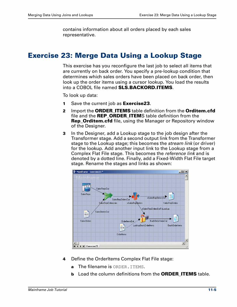
Merging Data Using Joins and Lookups Exercise 23: Merge Data Using a Lookup Stage
contains information about all orders placed by each sales
representative.
Exercise 23: Merge Data Using a Lookup StageThis exercise has you reconfigure the last job to select all items that
are currently on back order. You specify a pre-lookup condition that
determines which sales orders have been placed on back order, then
look up the order items using a cursor lookup. You load the results
into a COBOL file named SLS.BACKORD.ITEMS.
To look up data:
1 Save the current job as Exercise23.
2 Import the ORDER_ITEMS table definition from the Orditem.cfd file and the REP_ORDER_ITEMS table definition from the Rep_Orditem.cfd file, using the Manager or Repository window of the Designer.
3 In the Designer, add a Lookup stage to the job design after the Transformer stage. Add a second output link from the Transformer stage to the Lookup stage; this becomes the stream link (or driver) for the lookup. Add another input link to the Lookup stage from a Complex Flat File stage. This becomes the reference link and is denoted by a dotted line. Finally, add a Fixed-Width Flat File target stage. Rename the stages and links as shown:
4 Define the OrderItems Complex Flat File stage:
a The filename is ORDER.ITEMS.
b Load the column definitions from the ORDER_ITEMS table.
Mainframe Job Tutorial 11-5
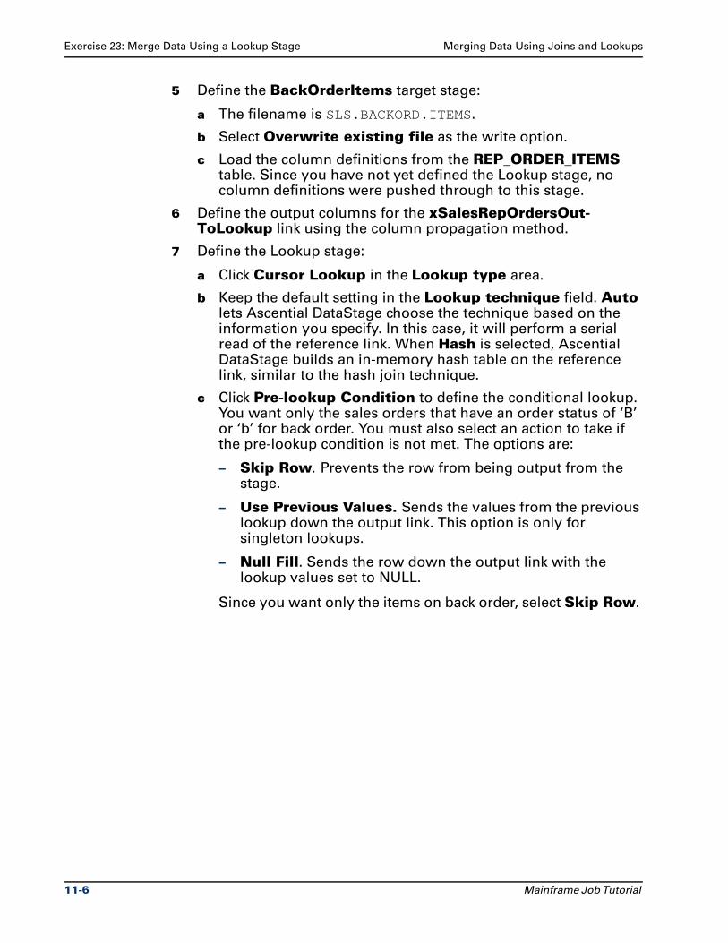
Exercise 23: Merge Data Using a Lookup Stage Merging Data Using Joins and Lookups
5 Define the BackOrderItems target stage:
a The filename is SLS.BACKORD.ITEMS.
b Select Overwrite existing file as the write option.
c Load the column definitions from the REP_ORDER_ITEMS table. Since you have not yet defined the Lookup stage, no column definitions were pushed through to this stage.
6 Define the output columns for the xSalesRepOrdersOut-ToLookup link using the column propagation method.
7 Define the Lookup stage:
a Click Cursor Lookup in the Lookup type area.
b Keep the default setting in the Lookup technique field. Auto lets Ascential DataStage choose the technique based on the information you specify. In this case, it will perform a serial read of the reference link. When Hash is selected, Ascential DataStage builds an in-memory hash table on the reference link, similar to the hash join technique.
c Click Pre-lookup Condition to define the conditional lookup. You want only the sales orders that have an order status of ‘B’ or ‘b’ for back order. You must also select an action to take if the pre-lookup condition is not met. The options are:
– Skip Row. Prevents the row from being output from the stage.
– Use Previous Values. Sends the values from the previous lookup down the output link. This option is only for singleton lookups.
– Null Fill. Sends the row down the output link with the lookup values set to NULL.
Since you want only the items on back order, select Skip Row.
11-6 Mainframe Job Tutorial
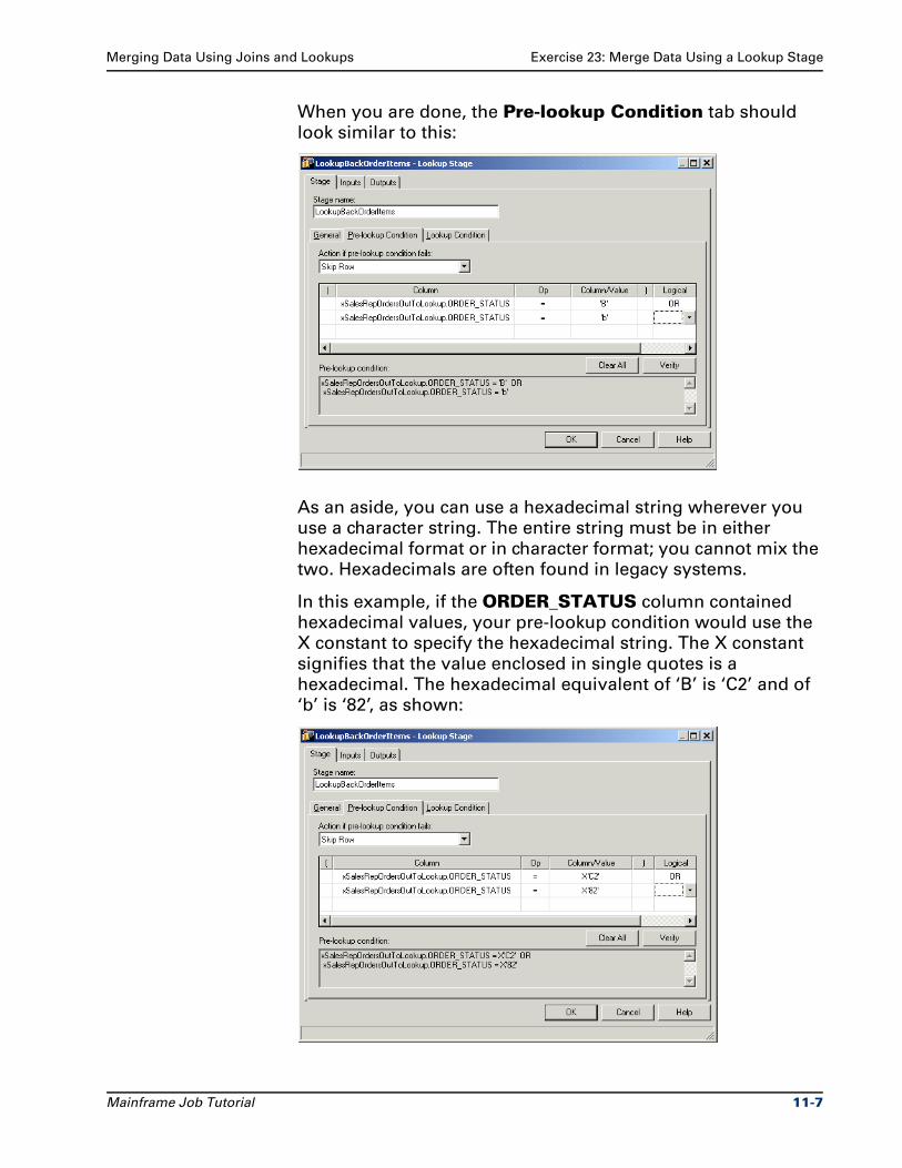
Merging Data Using Joins and Lookups Exercise 23: Merge Data Using a Lookup Stage
When you are done, the Pre-lookup Condition tab should
look similar to this:
As an aside, you can use a hexadecimal string wherever you
use a character string. The entire string must be in either
hexadecimal format or in character format; you cannot mix the
two. Hexadecimals are often found in legacy systems.
In this example, if the ORDER_STATUS column contained
hexadecimal values, your pre-lookup condition would use the
X constant to specify the hexadecimal string. The X constant
signifies that the value enclosed in single quotes is a
hexadecimal. The hexadecimal equivalent of ‘B’ is ‘C2’ and of
‘b’ is ‘82’, as shown:
Mainframe Job Tutorial 11-7
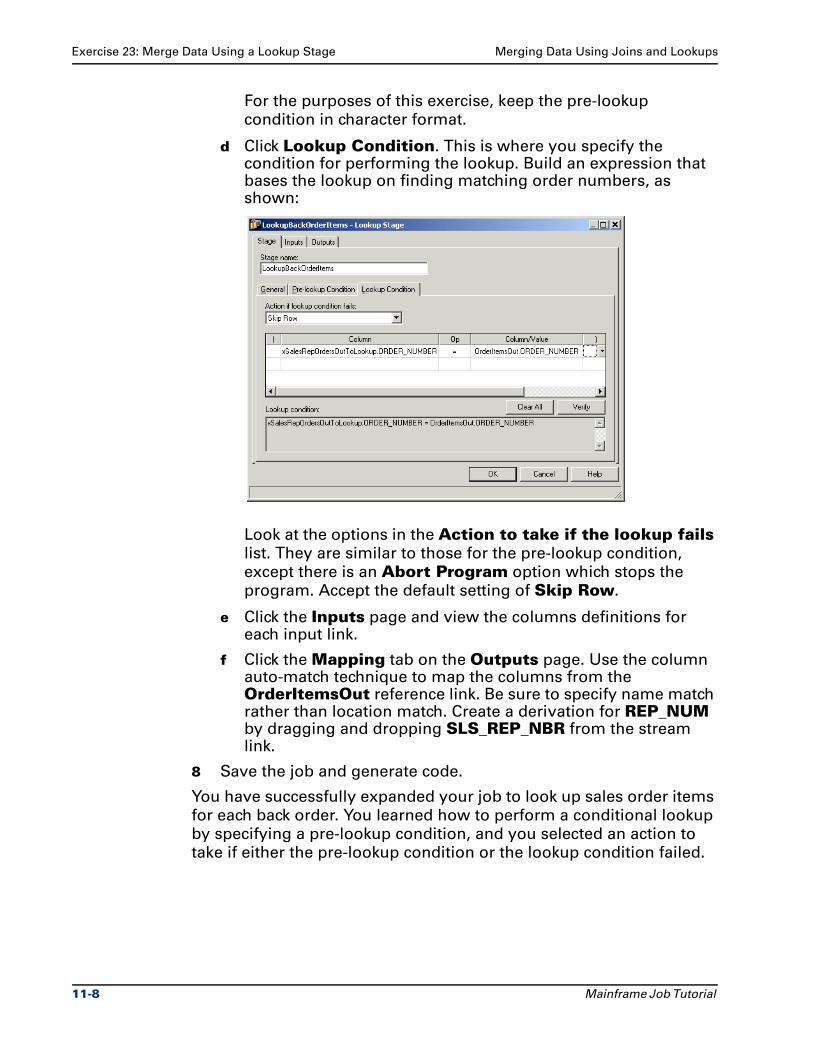
Exercise 23: Merge Data Using a Lookup Stage Merging Data Using Joins and Lookups
For the purposes of this exercise, keep the pre-lookup
condition in character format.
d Click Lookup Condition. This is where you specify the condition for performing the lookup. Build an expression that bases the lookup on finding matching order numbers, as shown:
Look at the options in the Action to take if the lookup fails
list. They are similar to those for the pre-lookup condition,
except there is an Abort Program option which stops the
program. Accept the default setting of Skip Row.
e Click the Inputs page and view the columns definitions for each input link.
f Click the Mapping tab on the Outputs page. Use the column auto-match technique to map the columns from the OrderItemsOut reference link. Be sure to specify name match rather than location match. Create a derivation for REP_NUM by dragging and dropping SLS_REP_NBR from the stream link.
8 Save the job and generate code.
You have successfully expanded your job to look up sales order items
for each back order. You learned how to perform a conditional lookup
by specifying a pre-lookup condition, and you selected an action to
take if either the pre-lookup condition or the lookup condition failed.
11-8 Mainframe Job Tutorial
Merging Data Using Joins and Lookups Summary
SummaryThis chapter took you through the process of merging data using Join
and Lookup stages. You became familiar with the types of joins and
lookups that can be performed, and you learned the differences
between the various join and lookup techniques that Ascential
DataStage provides. You also saw how to build the key expression
that determines the conditions under which a join or a lookup is
performed.
You are beginning to see the powerful capabilities that Ascential
DataStage offers for manipulating data. Next, you look at two more
active stage types that are used for aggregating and sorting data.
Mainframe Job Tutorial 11-9
12Sorting and Aggregating Data
In this chapter you learn two more ways to process data in mainframe
jobs: sorting and aggregating. These techniques are especially useful
for data warehousing because they allow you to group and
summarize data for easier analysis.
Sort stages allow you to sort data from a single input link. You can
select multiple columns to sort by. You then specify whether to sort
them in ascending or descending order.
Aggregator stages allow you to group and summarize data from a
single input link. You can perform a variety of aggregation functions
such as count, sum, average, first, last, min, and max.
Exercise 24 shows you how to sort data using Sort stages. You see
how to select sort columns and specify the sort order.
Exercise 25 introduces you to Aggregator stages. You learn about the
two methods of aggregating data and the different aggregation
functions that can be performed. You also see how to pre-sort your
source data as an alternative to using a Sort stage. When you use the
pre-sort function, Ascential DataStage generates an extra JCL step to
pre-sort the data prior to executing the generated COBOL program.
Exercise 26 demonstrates how to use DataStage’s ENDOFDATA
variable to perform special aggregation. You add an end-of-data row
to your source stage, then use this indicator in a Transformer stage
constraint to determine when the last row of input data has been
processed. A stage variable keeps a running total of revenue for all
products on back order, and sends the result to an output link after the
end-of-data flag is reached.
Mainframe Job Tutorial 12-1
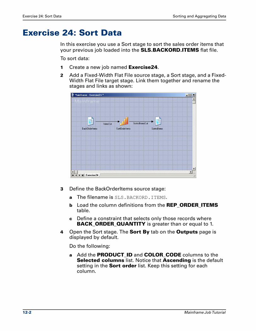
Exercise 24: Sort Data Sorting and Aggregating Data
Exercise 24: Sort DataIn this exercise you use a Sort stage to sort the sales order items that
your previous job loaded into the SLS.BACKORD.ITEMS flat file.
To sort data:
1 Create a new job named Exercise24.
2 Add a Fixed-Width Flat File source stage, a Sort stage, and a Fixed-Width Flat File target stage. Link them together and rename the stages and links as shown:
3 Define the BackOrderItems source stage:
a The filename is SLS.BACKORD.ITEMS.
b Load the column definitions from the REP_ORDER_ITEMS table.
c Define a constraint that selects only those records where BACK_ORDER_QUANTITY is greater than or equal to 1.
4 Open the Sort stage. The Sort By tab on the Outputs page is displayed by default.
Do the following:
a Add the PRODUCT_ID and COLOR_CODE columns to the Selected columns list. Notice that Ascending is the default setting in the Sort order list. Keep this setting for each column.
12-2 Mainframe Job Tutorial
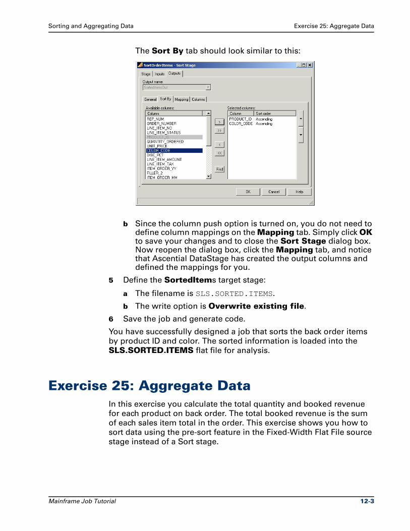
Sorting and Aggregating Data Exercise 25: Aggregate Data
The Sort By tab should look similar to this:
b Since the column push option is turned on, you do not need to define column mappings on the Mapping tab. Simply click OK to save your changes and to close the Sort Stage dialog box. Now reopen the dialog box, click the Mapping tab, and notice that Ascential DataStage has created the output columns and defined the mappings for you.
5 Define the SortedItems target stage:
a The filename is SLS.SORTED.ITEMS.
b The write option is Overwrite existing file.
6 Save the job and generate code.
You have successfully designed a job that sorts the back order items
by product ID and color. The sorted information is loaded into the
SLS.SORTED.ITEMS flat file for analysis.
Exercise 25: Aggregate DataIn this exercise you calculate the total quantity and booked revenue
for each product on back order. The total booked revenue is the sum
of each sales item total in the order. This exercise shows you how to
sort data using the pre-sort feature in the Fixed-Width Flat File source
stage instead of a Sort stage.
Mainframe Job Tutorial 12-3
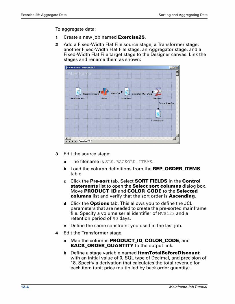
Exercise 25: Aggregate Data Sorting and Aggregating Data
To aggregate data:
1 Create a new job named Exercise25.
2 Add a Fixed-Width Flat File source stage, a Transformer stage, another Fixed-Width Flat File stage, an Aggregator stage, and a Fixed-Width Flat File target stage to the Designer canvas. Link the stages and rename them as shown:
3 Edit the source stage:
a The filename is SLS.BACKORD.ITEMS.
b Load the column definitions from the REP_ORDER_ITEMS table.
c Click the Pre-sort tab. Select SORT FIELDS in the Control statements list to open the Select sort columns dialog box. Move PRODUCT_ID and COLOR_CODE to the Selected columns list and verify that the sort order is Ascending.
d Click the Options tab. This allows you to define the JCL parameters that are needed to create the pre-sorted mainframe file. Specify a volume serial identifier of MVS123 and a retention period of 90 days.
e Define the same constraint you used in the last job.
4 Edit the Transformer stage:
a Map the columns PRODUCT_ID, COLOR_CODE, and BACK_ORDER_QUANTITY to the output link.
b Define a stage variable named ItemTotalBeforeDiscount with an initial value of 0, SQL type of Decimal, and precision of 18. Specify a derivation that calculates the total revenue for each item (unit price multiplied by back order quantity).
12-4 Mainframe Job Tutorial
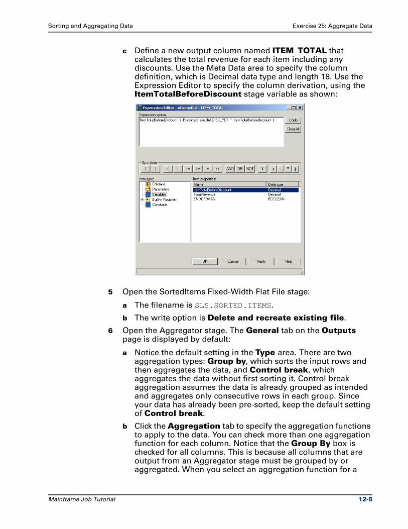
Sorting and Aggregating Data Exercise 25: Aggregate Data
c Define a new output column named ITEM_TOTAL that calculates the total revenue for each item including any discounts. Use the Meta Data area to specify the column definition, which is Decimal data type and length 18. Use the Expression Editor to specify the column derivation, using the ItemTotalBeforeDiscount stage variable as shown:
5 Open the SortedItems Fixed-Width Flat File stage:
a The filename is SLS.SORTED.ITEMS.
b The write option is Delete and recreate existing file.
6 Open the Aggregator stage. The General tab on the Outputs page is displayed by default:
a Notice the default setting in the Type area. There are two aggregation types: Group by, which sorts the input rows and then aggregates the data, and Control break, which aggregates the data without first sorting it. Control break aggregation assumes the data is already grouped as intended and aggregates only consecutive rows in each group. Since your data has already been pre-sorted, keep the default setting of Control break.
b Click the Aggregation tab to specify the aggregation functions to apply to the data. You can check more than one aggregation function for each column. Notice that the Group By box is checked for all columns. This is because all columns that are output from an Aggregator stage must be grouped by or aggregated. When you select an aggregation function for a
Mainframe Job Tutorial 12-5
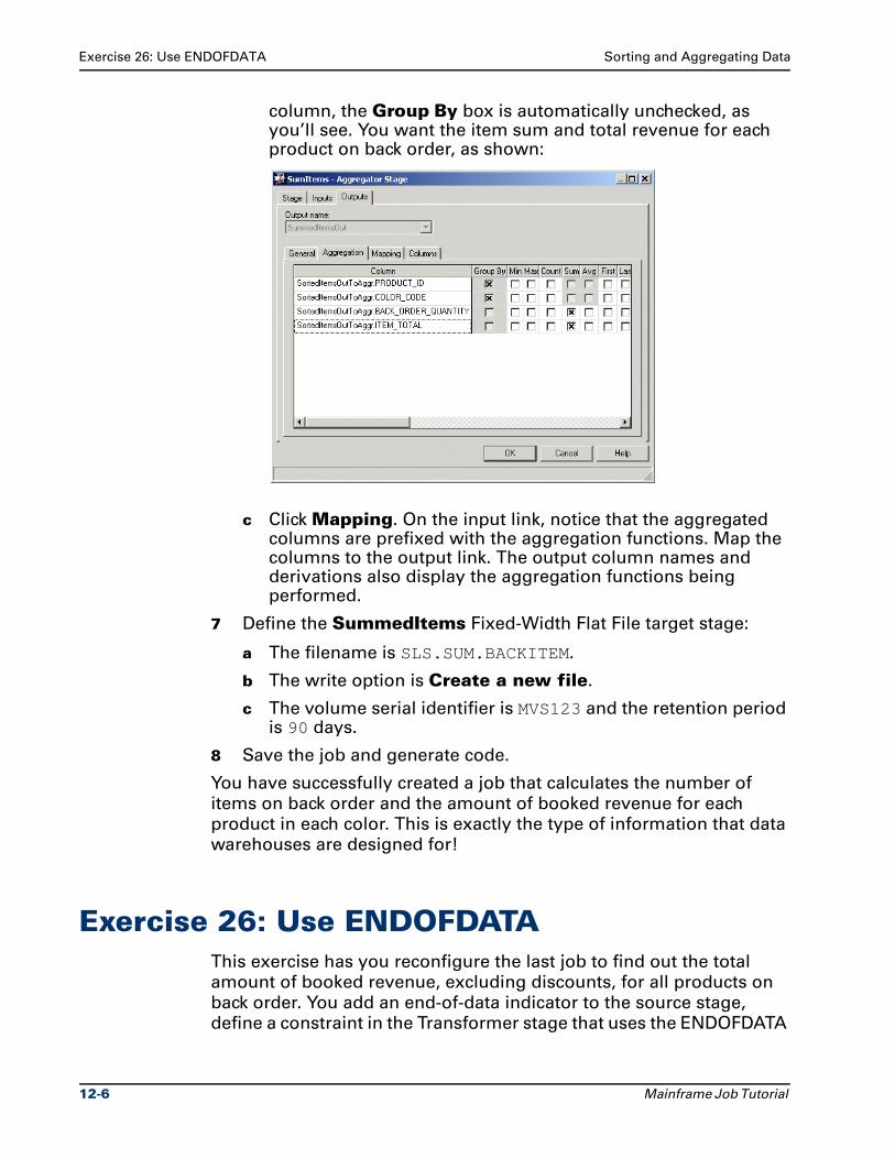
Exercise 26: Use ENDOFDATA Sorting and Aggregating Data
column, the Group By box is automatically unchecked, as you’ll see. You want the item sum and total revenue for each product on back order, as shown:
c Click Mapping. On the input link, notice that the aggregated columns are prefixed with the aggregation functions. Map the columns to the output link. The output column names and derivations also display the aggregation functions being performed.
7 Define the SummedItems Fixed-Width Flat File target stage:
a The filename is SLS.SUM.BACKITEM.
b The write option is Create a new file.
c The volume serial identifier is MVS123 and the retention period is 90 days.
8 Save the job and generate code.
You have successfully created a job that calculates the number of
items on back order and the amount of booked revenue for each
product in each color. This is exactly the type of information that data
warehouses are designed for!
Exercise 26: Use ENDOFDATAThis exercise has you reconfigure the last job to find out the total
amount of booked revenue, excluding discounts, for all products on
back order. You add an end-of-data indicator to the source stage,
define a constraint in the Transformer stage that uses the ENDOFDATA
12-6 Mainframe Job Tutorial
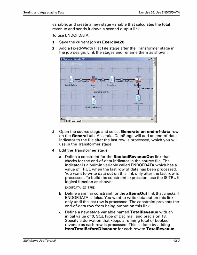
Sorting and Aggregating Data Exercise 26: Use ENDOFDATA
variable, and create a new stage variable that calculates the total
revenue and sends it down a second output link.
To use ENDOFDATA:
1 Save the current job as Exercise26.
2 Add a Fixed-Width Flat File stage after the Transformer stage in the job design. Link the stages and rename them as shown:
3 Open the source stage and select Generate an end-of-data row on the General tab. Ascential DataStage will add an end-of-data indicator to the file after the last row is processed, which you will use in the Transformer stage.
4 Edit the Transformer stage:
a Define a constraint for the BookedRevenueOut link that checks for the end-of-data indicator in the source file. The indicator is a built-in variable called ENDOFDATA which has a value of TRUE when the last row of data has been processed. You want to write data out on this link only after the last row is processed. To build the constraint expression, use the IS TRUE logical function as shown:
ENDOFDATA IS TRUE
b Define a similar constraint for the xItemsOut link that checks if ENDOFDATA is false. You want to write data out on this link only until the last row is processed. The constraint prevents the end-of-data row from being output on this link.
c Define a new stage variable named TotalRevenue with an initial value of 0, SQL type of Decimal, and precision 18. Specify a derivation that keeps a running total of booked revenue as each row is processed. This is done by adding ItemTotalBeforeDiscount for each row to TotalRevenue.
Mainframe Job Tutorial 12-7
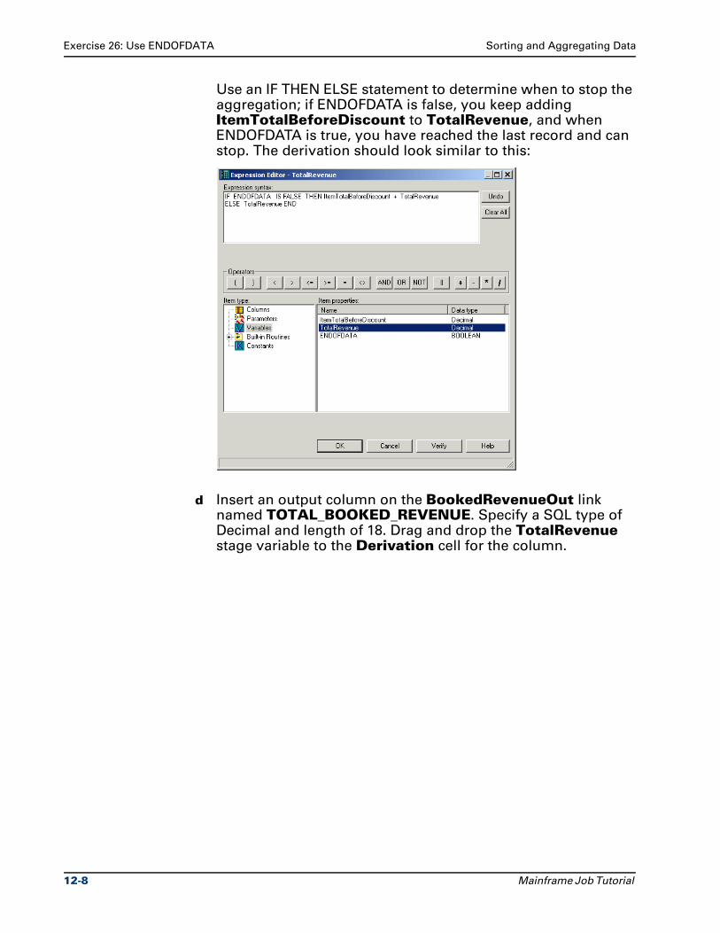
Exercise 26: Use ENDOFDATA Sorting and Aggregating Data
Use an IF THEN ELSE statement to determine when to stop the aggregation; if ENDOFDATA is false, you keep adding ItemTotalBeforeDiscount to TotalRevenue, and when ENDOFDATA is true, you have reached the last record and can stop. The derivation should look similar to this:
d Insert an output column on the BookedRevenueOut link named TOTAL_BOOKED_REVENUE. Specify a SQL type of Decimal and length of 18. Drag and drop the TotalRevenue stage variable to the Derivation cell for the column.
12-8 Mainframe Job Tutorial
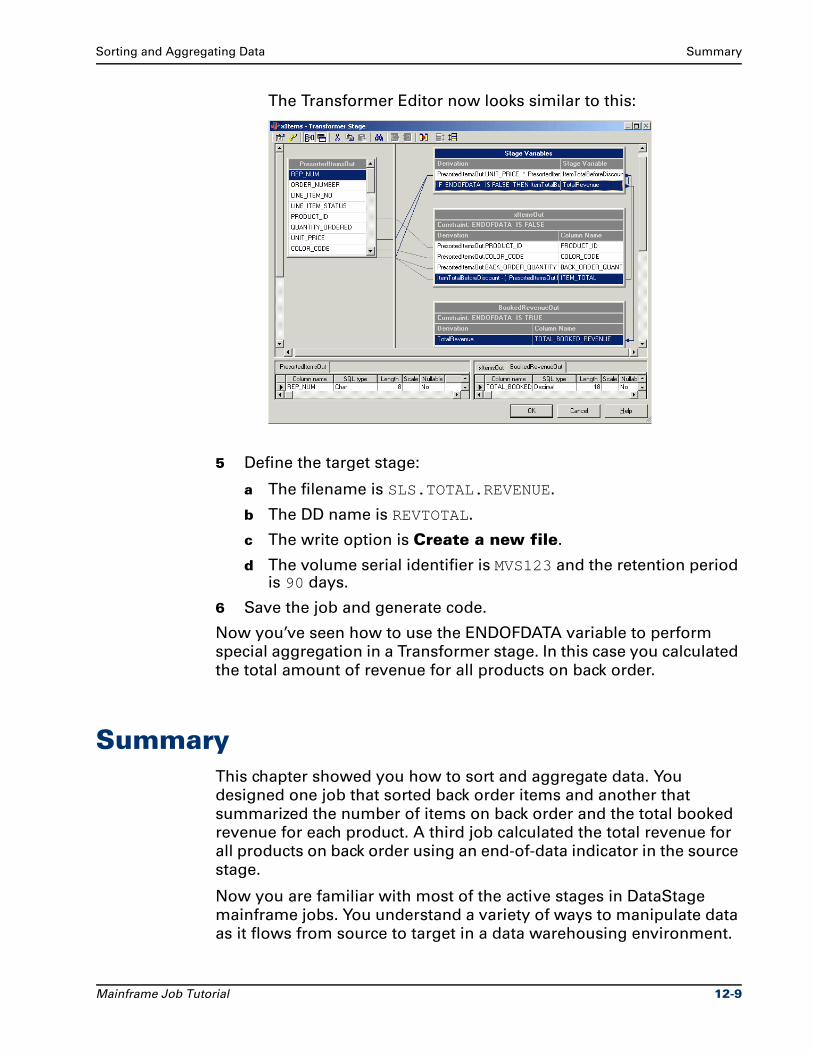
Sorting and Aggregating Data Summary
The Transformer Editor now looks similar to this:
5 Define the target stage:
a The filename is SLS.TOTAL.REVENUE.
b The DD name is REVTOTAL.
c The write option is Create a new file.
d The volume serial identifier is MVS123 and the retention period is 90 days.
6 Save the job and generate code.
Now you’ve seen how to use the ENDOFDATA variable to perform
special aggregation in a Transformer stage. In this case you calculated
the total amount of revenue for all products on back order.
SummaryThis chapter showed you how to sort and aggregate data. You
designed one job that sorted back order items and another that
summarized the number of items on back order and the total booked
revenue for each product. A third job calculated the total revenue for
all products on back order using an end-of-data indicator in the source
stage.
Now you are familiar with most of the active stages in DataStage
mainframe jobs. You understand a variety of ways to manipulate data
as it flows from source to target in a data warehousing environment.
Mainframe Job Tutorial 12-9
Summary Sorting and Aggregating Data
In the next chapter, you learn how to specify more complex data
transformations using SQL business rule logic.
12-10 Mainframe Job Tutorial
13Defining Business Rules
This chapter shows you how to use Business Rule stages to define
complex data transformations in mainframe jobs. Business Rule
stages are similar to Transformer stages in two ways:
They allow you to define stage variables.
They have a built-in editor, similar to the Expression Editor, where you specify SQL business rule logic.
The main difference is that Business Rule stages provide access to the
control-flow features of SQL, such as conditional and looping
statements. This allows you to perform conditional mappings and
looping transformations in your jobs. You can also use SQL’s COMMIT
and ROLLBACK statements, allowing for greater transaction control in
jobs with relational databases.
Exercise 27 demonstrates how to use a Business Rule stage for
transaction control. You redesign a job from Chapter 9 that has a
Relational target stage. You add a Business Rule stage to determine
whether the updates to the target table are made successfully or not.
If so, the changes are committed. If not, the changes are rolled back
and the job is terminated.
Exercise 27: Controlling Relational TransactionsThis exercise has you redesign the job from Exercise 19 to determine
when to commit or roll back changes to the target table. You use a
Business Rule stage to specify the necessary business rule logic.
Mainframe Job Tutorial 13-1
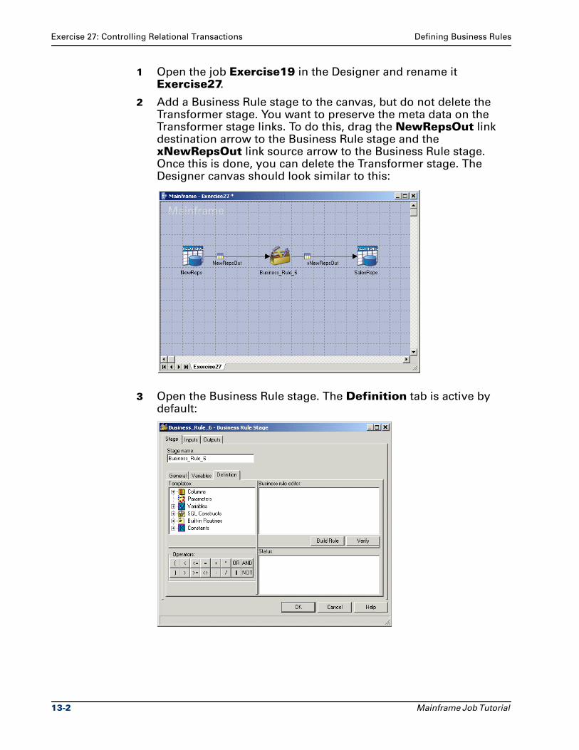
Exercise 27: Controlling Relational Transactions Defining Business Rules
1 Open the job Exercise19 in the Designer and rename it Exercise27.
2 Add a Business Rule stage to the canvas, but do not delete the Transformer stage. You want to preserve the meta data on the Transformer stage links. To do this, drag the NewRepsOut link destination arrow to the Business Rule stage and the xNewRepsOut link source arrow to the Business Rule stage. Once this is done, you can delete the Transformer stage. The Designer canvas should look similar to this:
3 Open the Business Rule stage. The Definition tab is active by default:
13-2 Mainframe Job Tutorial
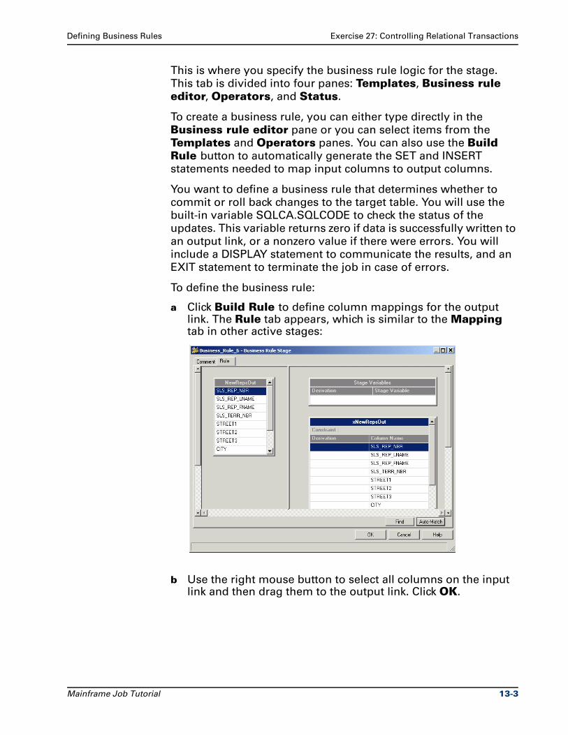
Defining Business Rules Exercise 27: Controlling Relational Transactions
This is where you specify the business rule logic for the stage.
This tab is divided into four panes: Templates, Business rule editor, Operators, and Status.
To create a business rule, you can either type directly in the
Business rule editor pane or you can select items from the
Templates and Operators panes. You can also use the Build Rule button to automatically generate the SET and INSERT
statements needed to map input columns to output columns.
You want to define a business rule that determines whether to
commit or roll back changes to the target table. You will use the
built-in variable SQLCA.SQLCODE to check the status of the
updates. This variable returns zero if data is successfully written to
an output link, or a nonzero value if there were errors. You will
include a DISPLAY statement to communicate the results, and an
EXIT statement to terminate the job in case of errors.
To define the business rule:
a Click Build Rule to define column mappings for the output link. The Rule tab appears, which is similar to the Mapping tab in other active stages:
b Use the right mouse button to select all columns on the input link and then drag them to the output link. Click OK.
Mainframe Job Tutorial 13-3
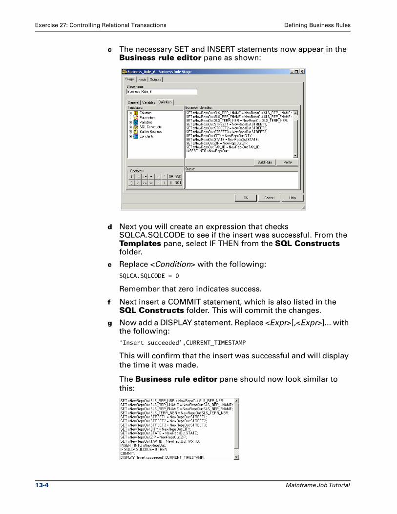
Exercise 27: Controlling Relational Transactions Defining Business Rules
c The necessary SET and INSERT statements now appear in the Business rule editor pane as shown:
d Next you will create an expression that checks SQLCA.SQLCODE to see if the insert was successful. From the Templates pane, select IF THEN from the SQL Constructs folder.
e Replace <Condition> with the following:
SQLCA.SQLCODE = 0
Remember that zero indicates success.
f Next insert a COMMIT statement, which is also listed in the SQL Constructs folder. This will commit the changes.
g Now add a DISPLAY statement. Replace <Expr>[,<Expr>]... with the following:
‘Insert succeeded’,CURRENT_TIMESTAMP
This will confirm that the insert was successful and will display
the time it was made.
The Business rule editor pane should now look similar to
this:
13-4 Mainframe Job Tutorial
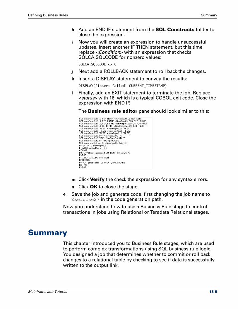
Defining Business Rules Summary
h Add an END IF statement from the SQL Constructs folder to close the expression.
i Now you will create an expression to handle unsuccessful updates. Insert another IF THEN statement, but this time replace <Condition> with an expression that checks SQLCA.SQLCODE for nonzero values:
SQLCA.SQLCODE <> 0
j Next add a ROLLBACK statement to roll back the changes.
k Insert a DISPLAY statement to convey the results:
DISPLAY(‘Insert failed’,CURRENT_TIMESTAMP)
l Finally, add an EXIT statement to terminate the job. Replace <status> with 16, which is a typical COBOL exit code. Close the expression with END IF.
The Business rule editor pane should look similar to this:
m Click Verify the check the expression for any syntax errors.
n Click OK to close the stage.
4 Save the job and generate code, first changing the job name to Exercise27 in the code generation path.
Now you understand how to use a Business Rule stage to control
transactions in jobs using Relational or Teradata Relational stages.
SummaryThis chapter introduced you to Business Rule stages, which are used
to perform complex transformations using SQL business rule logic.
You designed a job that determines whether to commit or roll back
changes to a relational table by checking to see if data is successfully
written to the output link.
Mainframe Job Tutorial 13-5
Summary Defining Business Rules
Next you explore one more active stage that provides the means for
incorporating more advanced programming into your mainframe
jobs.
13-6 Mainframe Job Tutorial
14Calling External Routines
One of the most powerful features of Ascential DataStage Enterprise
MVS Edition is the ability to call external COBOL subroutines in your
jobs. This allows you to incorporate complex processing or
functionality specific to your environment in the DataStage-generated
programs. The external routine can be written in any language that
can be called by a COBOL program, such as COBOL, Assembler, or C.
This chapter shows you how to define and call external routines in
mainframe jobs. You first define the routine meta data in the
DataStage Manager, recalling what you learned in Chapter 10. Then
you use an External Routine stage to call the routine and map its input
and output arguments.
Exercise 28: Define Routine Meta DataIn this exercise you create a routine definition in the DataStage
Manager, similar to those you created for external source and external
target programs. The routine definition includes the name, library
path, invocation method, and input and output arguments for an
external routine named DATEDIF, which calculates the number of
days between two dates. The routine definition is then stored in the
DataStage Repository and can be used in any mainframe job.
To define the routine meta data:
1 Open the Mainframe Routine dialog box in the Manager and specify the following on the General page:
a The routine name is DATEDIF.
b The routine type is External Routine.
Mainframe Job Tutorial 14-1
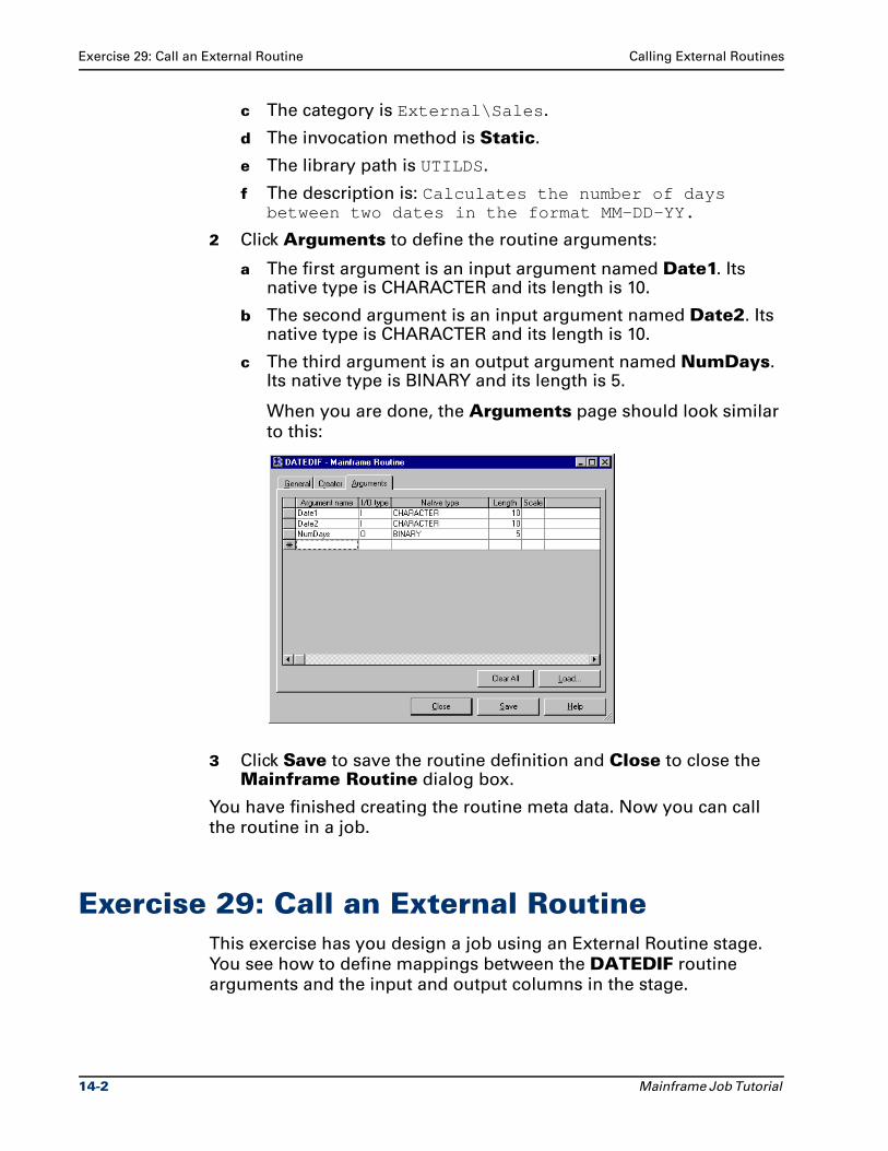
Exercise 29: Call an External Routine Calling External Routines
c The category is External\Sales.
d The invocation method is Static.
e The library path is UTILDS.
f The description is: Calculates the number of days between two dates in the format MM-DD-YY.
2 Click Arguments to define the routine arguments:
a The first argument is an input argument named Date1. Its native type is CHARACTER and its length is 10.
b The second argument is an input argument named Date2. Its native type is CHARACTER and its length is 10.
c The third argument is an output argument named NumDays. Its native type is BINARY and its length is 5.
When you are done, the Arguments page should look similar
to this:
3 Click Save to save the routine definition and Close to close the Mainframe Routine dialog box.
You have finished creating the routine meta data. Now you can call
the routine in a job.
Exercise 29: Call an External RoutineThis exercise has you design a job using an External Routine stage.
You see how to define mappings between the DATEDIF routine
arguments and the input and output columns in the stage.
14-2 Mainframe Job Tutorial
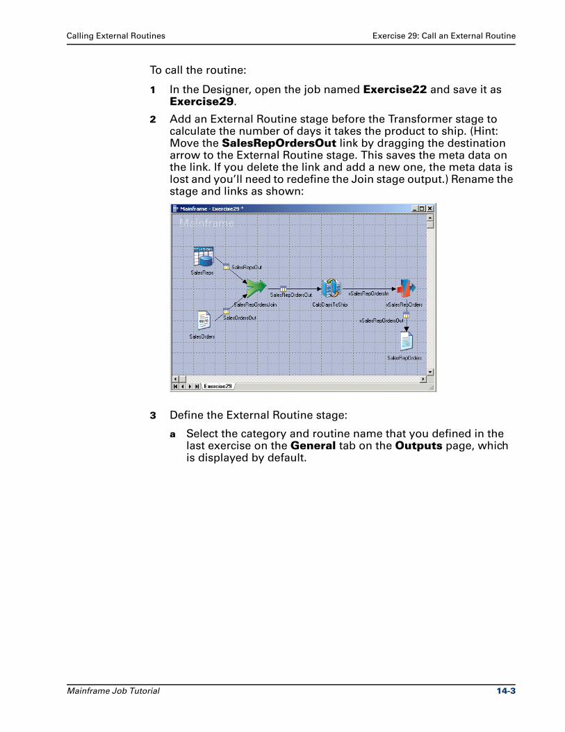
Calling External Routines Exercise 29: Call an External Routine
To call the routine:
1 In the Designer, open the job named Exercise22 and save it as Exercise29.
2 Add an External Routine stage before the Transformer stage to calculate the number of days it takes the product to ship. (Hint: Move the SalesRepOrdersOut link by dragging the destination arrow to the External Routine stage. This saves the meta data on the link. If you delete the link and add a new one, the meta data is lost and you’ll need to redefine the Join stage output.) Rename the stage and links as shown:
3 Define the External Routine stage:
a Select the category and routine name that you defined in the last exercise on the General tab on the Outputs page, which is displayed by default.
Mainframe Job Tutorial 14-3
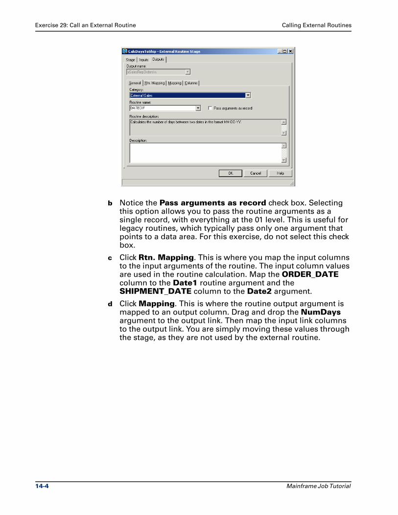
Exercise 29: Call an External Routine Calling External Routines
b Notice the Pass arguments as record check box. Selecting this option allows you to pass the routine arguments as a single record, with everything at the 01 level. This is useful for legacy routines, which typically pass only one argument that points to a data area. For this exercise, do not select this check box.
c Click Rtn. Mapping. This is where you map the input columns to the input arguments of the routine. The input column values are used in the routine calculation. Map the ORDER_DATE column to the Date1 routine argument and the SHIPMENT_DATE column to the Date2 argument.
d Click Mapping. This is where the routine output argument is mapped to an output column. Drag and drop the NumDays argument to the output link. Then map the input link columns to the output link. You are simply moving these values through the stage, as they are not used by the external routine.
14-4 Mainframe Job Tutorial
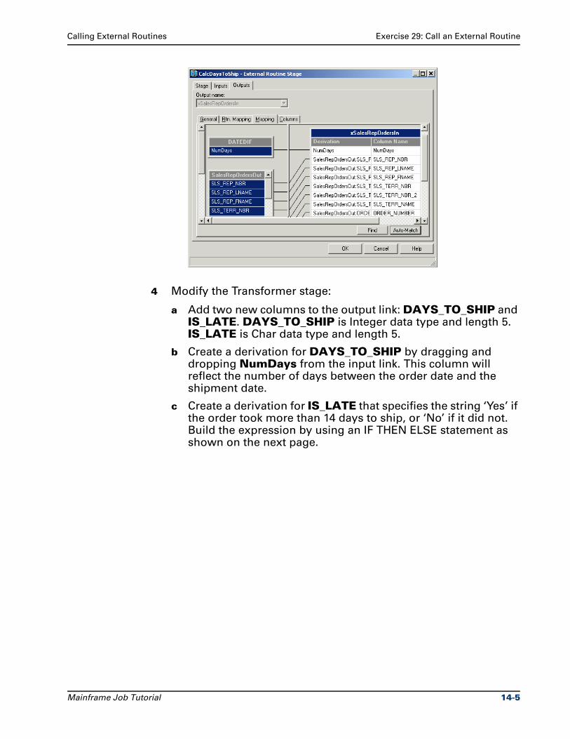
Calling External Routines Exercise 29: Call an External Routine
4 Modify the Transformer stage:
a Add two new columns to the output link: DAYS_TO_SHIP and IS_LATE. DAYS_TO_SHIP is Integer data type and length 5. IS_LATE is Char data type and length 5.
b Create a derivation for DAYS_TO_SHIP by dragging and dropping NumDays from the input link. This column will reflect the number of days between the order date and the shipment date.
c Create a derivation for IS_LATE that specifies the string ‘Yes’ if the order took more than 14 days to ship, or ‘No’ if it did not. Build the expression by using an IF THEN ELSE statement as shown on the next page.
Mainframe Job Tutorial 14-5
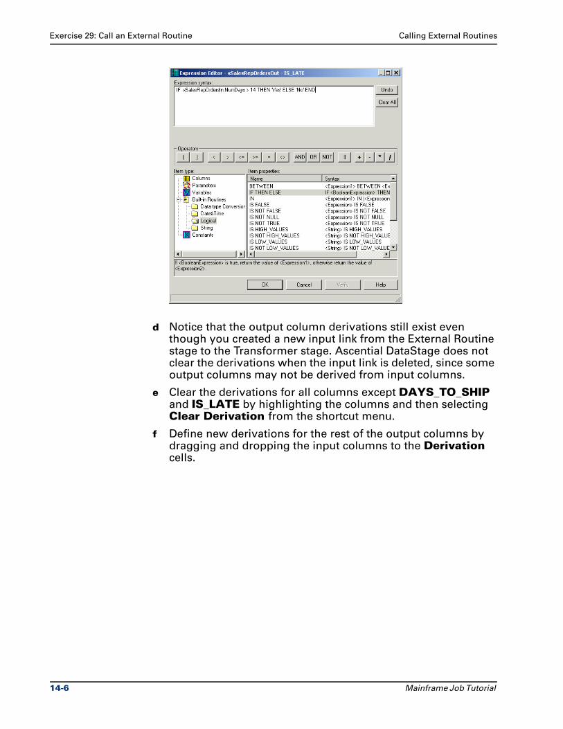
Exercise 29: Call an External Routine Calling External Routines
d Notice that the output column derivations still exist even though you created a new input link from the External Routine stage to the Transformer stage. Ascential DataStage does not clear the derivations when the input link is deleted, since some output columns may not be derived from input columns.
e Clear the derivations for all columns except DAYS_TO_SHIP and IS_LATE by highlighting the columns and then selecting Clear Derivation from the shortcut menu.
f Define new derivations for the rest of the output columns by dragging and dropping the input columns to the Derivation cells.
14-6 Mainframe Job Tutorial
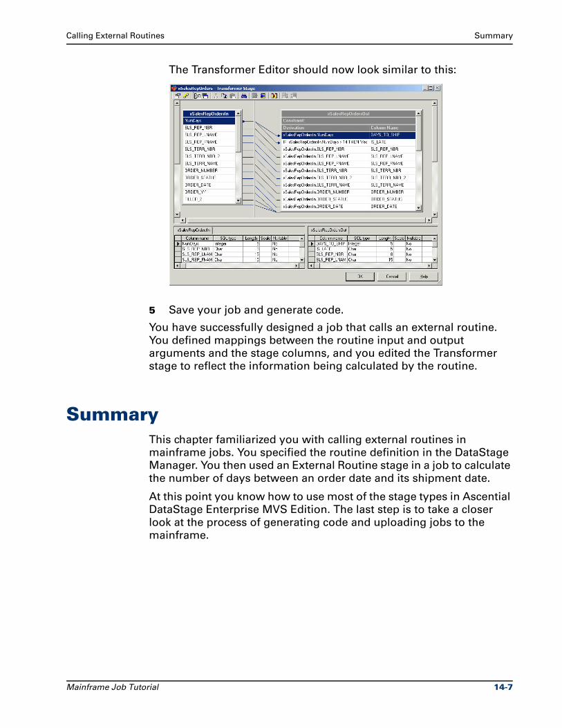
Calling External Routines Summary
The Transformer Editor should now look similar to this:
5 Save your job and generate code.
You have successfully designed a job that calls an external routine.
You defined mappings between the routine input and output
arguments and the stage columns, and you edited the Transformer
stage to reflect the information being calculated by the routine.
SummaryThis chapter familiarized you with calling external routines in
mainframe jobs. You specified the routine definition in the DataStage
Manager. You then used an External Routine stage in a job to calculate
the number of days between an order date and its shipment date.
At this point you know how to use most of the stage types in Ascential
DataStage Enterprise MVS Edition. The last step is to take a closer
look at the process of generating code and uploading jobs to the
mainframe.
Mainframe Job Tutorial 14-7
15Generating Code
When you finish designing a mainframe job in Ascential DataStage
Enterprise MVS Edition, you generate code. Three files are created:
COBOL source, compile JCL, and run JCL. These files are stored in a
directory on the DataStage client machine. You then upload the files to
the mainframe, where they are compiled and run.
The compile JCL invokes the COBOL compiler and link-editor on the
mainframe, and the run JCL executes the COBOL program. The
COBOL program extracts the source data, transforms it, and loads it to
the target data files or DB2 tables as specified in your job.
This chapter focuses on the process of generating code and uploading
jobs to the mainframe. In Exercise 30 you learn how to modify
DataStage’s JCL templates. Exercise 31 has you validate a job and
generate code. In Exercise 32 you define a machine profile in the
DataStage Manager. Finally, Exercise 33 walks you through a
simulated job upload.
Exercise 30: Modify JCL TemplatesJob Control Language (JCL) provides a set of instructions to the
mainframe on how to execute a job. It divides a job into one or more
steps that identify:
The program to be executed
The libraries containing the program
The files required by the program and their attributes
Any inline input required by the program
Conditions for performing a step
Mainframe Job Tutorial 15-1
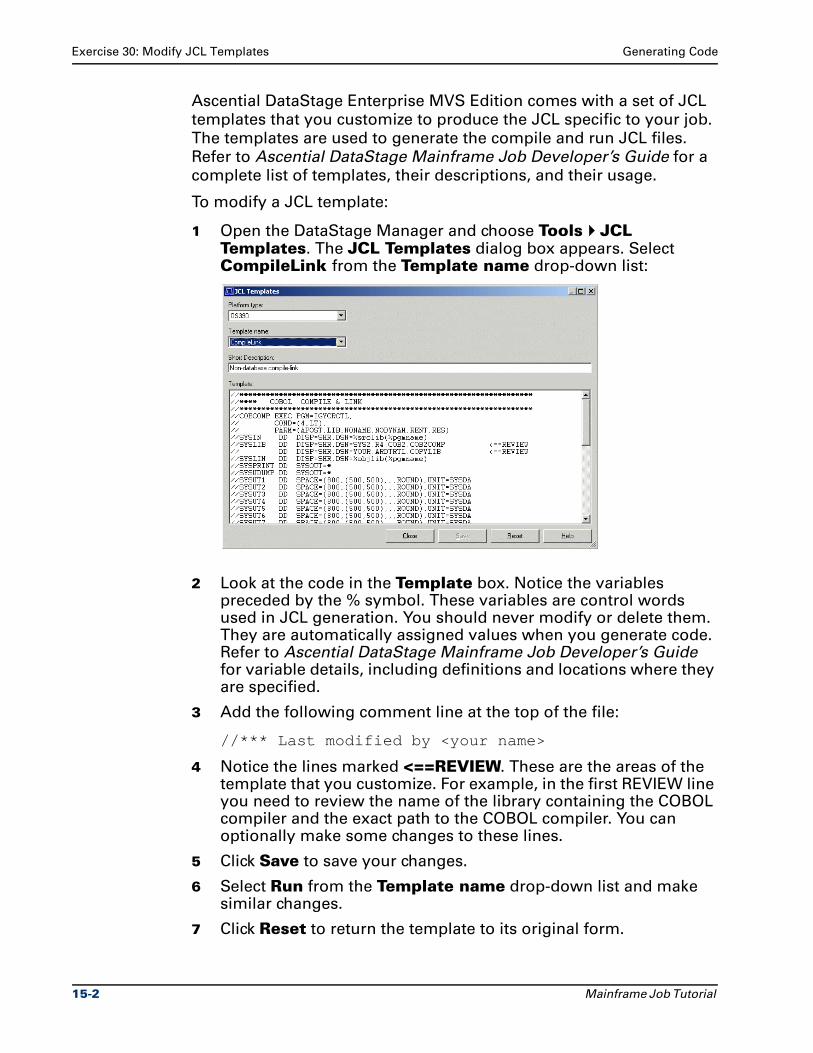
Exercise 30: Modify JCL Templates Generating Code
Ascential DataStage Enterprise MVS Edition comes with a set of JCL
templates that you customize to produce the JCL specific to your job.
The templates are used to generate the compile and run JCL files.
Refer to Ascential DataStage Mainframe Job Developer’s Guide for a
complete list of templates, their descriptions, and their usage.
To modify a JCL template:
1 Open the DataStage Manager and choose Tools JCL Templates. The JCL Templates dialog box appears. Select CompileLink from the Template name drop-down list:
2 Look at the code in the Template box. Notice the variables preceded by the % symbol. These variables are control words used in JCL generation. You should never modify or delete them. They are automatically assigned values when you generate code. Refer to Ascential DataStage Mainframe Job Developer’s Guide for variable details, including definitions and locations where they are specified.
3 Add the following comment line at the top of the file:
//*** Last modified by <your name>
4 Notice the lines marked <==REVIEW. These are the areas of the template that you customize. For example, in the first REVIEW line you need to review the name of the library containing the COBOL compiler and the exact path to the COBOL compiler. You can optionally make some changes to these lines.
5 Click Save to save your changes.
6 Select Run from the Template name drop-down list and make similar changes.
7 Click Reset to return the template to its original form.
15-2 Mainframe Job Tutorial
Generating Code Exercise 31: Validate a Job and Generate Code
8 Open the OldFile template and find the JCL variables.
9 Click Close.
You have seen how easy it is to customize a JCL template.
Exercise 31: Validate a Job and Generate CodeThough you have already seen how to generate code for your jobs,
this exercise has you take a closer look at the job validation and code
generation process.
When you generate code for a job, Ascential DataStage first validates
your job design. Validation of a mainframe job design involves:
Checking that all stages in the job are connected in one continuous flow and that each stage has the required number of input and output links
Checking the expressions used in each stage for syntax and semantic correctness
Checking the column mappings to ensure they are data-type compatible
The validation rules for mainframe jobs include the following:
Only one chain of stages is allowed in a job.
Every job must have at least one active stage.
Passive stages cannot be linked to passive stages.
Every stage must have at least one link.
Active stages must have at least one input link and one output link.
DD names must be unique within a job.
Output files created in a job must be unique.
For details about the links allowed between mainframe stage types
and the number of input and output links permitted in each stage,
refer to Ascential DataStage Mainframe Job Developer’s Guide.
To validate a job and generate code:
1 Open the job Exercise4 in the Designer.
2 Open the source stage and make a note of the filename and DD name.
3 Open the target stage and make a note of the filename and DD name.
Mainframe Job Tutorial 15-3
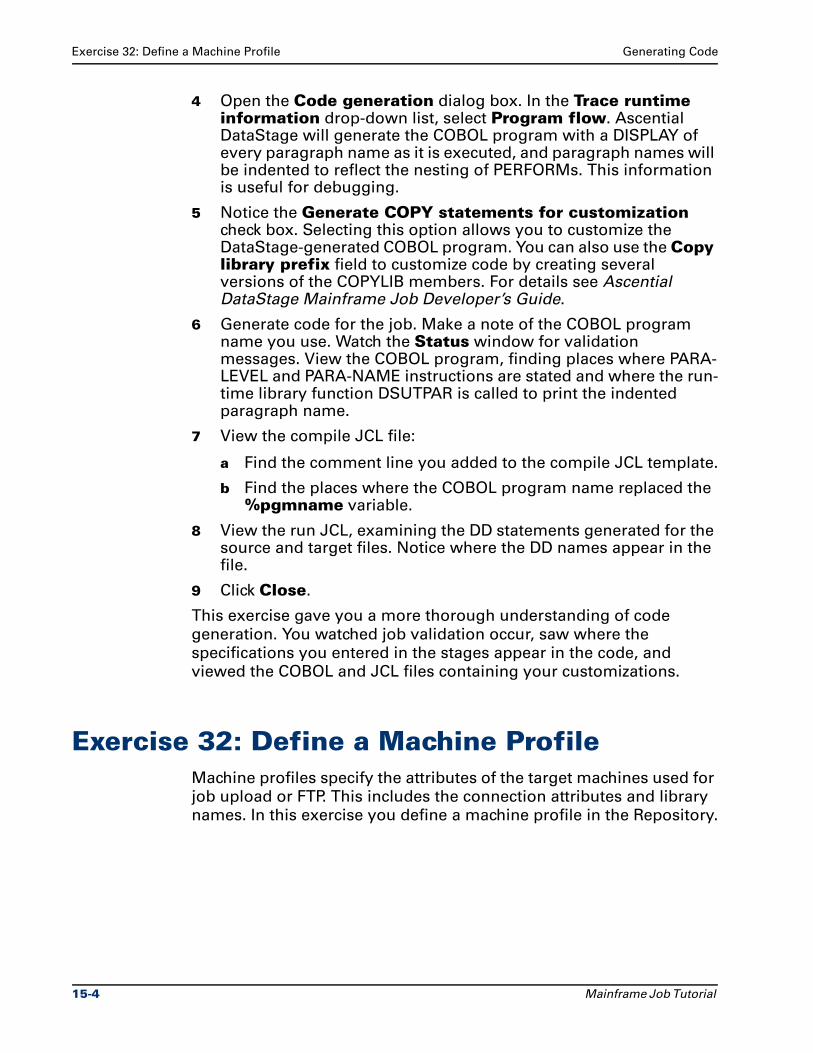
Exercise 32: Define a Machine Profile Generating Code
4 Open the Code generation dialog box. In the Trace runtime information drop-down list, select Program flow. Ascential DataStage will generate the COBOL program with a DISPLAY of every paragraph name as it is executed, and paragraph names will be indented to reflect the nesting of PERFORMs. This information is useful for debugging.
5 Notice the Generate COPY statements for customization check box. Selecting this option allows you to customize the DataStage-generated COBOL program. You can also use the Copy library prefix field to customize code by creating several versions of the COPYLIB members. For details see Ascential DataStage Mainframe Job Developer’s Guide.
6 Generate code for the job. Make a note of the COBOL program name you use. Watch the Status window for validation messages. View the COBOL program, finding places where PARA-LEVEL and PARA-NAME instructions are stated and where the run-time library function DSUTPAR is called to print the indented paragraph name.
7 View the compile JCL file:
a Find the comment line you added to the compile JCL template.
b Find the places where the COBOL program name replaced the %pgmname variable.
8 View the run JCL, examining the DD statements generated for the source and target files. Notice where the DD names appear in the file.
9 Click Close.
This exercise gave you a more thorough understanding of code
generation. You watched job validation occur, saw where the
specifications you entered in the stages appear in the code, and
viewed the COBOL and JCL files containing your customizations.
Exercise 32: Define a Machine ProfileMachine profiles specify the attributes of the target machines used for
job upload or FTP. This includes the connection attributes and library
names. In this exercise you define a machine profile in the Repository.
15-4 Mainframe Job Tutorial
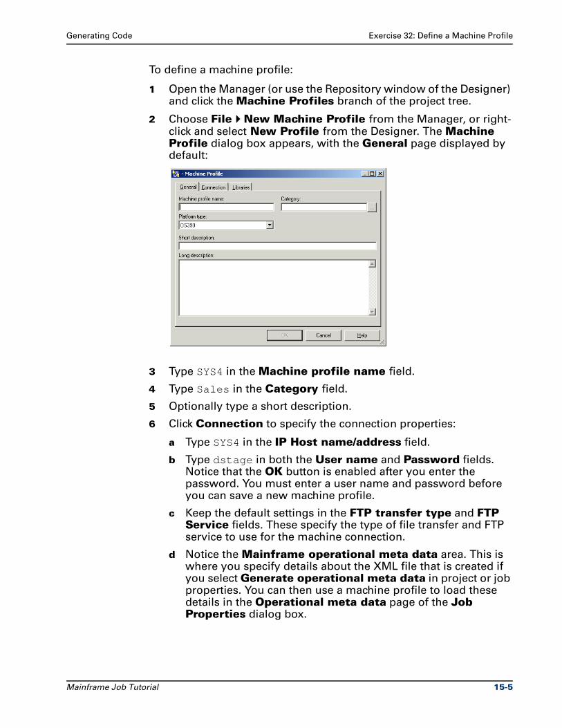
Generating Code Exercise 32: Define a Machine Profile
To define a machine profile:
1 Open the Manager (or use the Repository window of the Designer) and click the Machine Profiles branch of the project tree.
2 Choose File New Machine Profile from the Manager, or right-click and select New Profile from the Designer. The Machine Profile dialog box appears, with the General page displayed by default:
3 Type SYS4 in the Machine profile name field.
4 Type Sales in the Category field.
5 Optionally type a short description.
6 Click Connection to specify the connection properties:
a Type SYS4 in the IP Host name/address field.
b Type dstage in both the User name and Password fields. Notice that the OK button is enabled after you enter the password. You must enter a user name and password before you can save a new machine profile.
c Keep the default settings in the FTP transfer type and FTP Service fields. These specify the type of file transfer and FTP service to use for the machine connection.
d Notice the Mainframe operational meta data area. This is where you specify details about the XML file that is created if you select Generate operational meta data in project or job properties. You can then use a machine profile to load these details in the Operational meta data page of the Job Properties dialog box.
Mainframe Job Tutorial 15-5
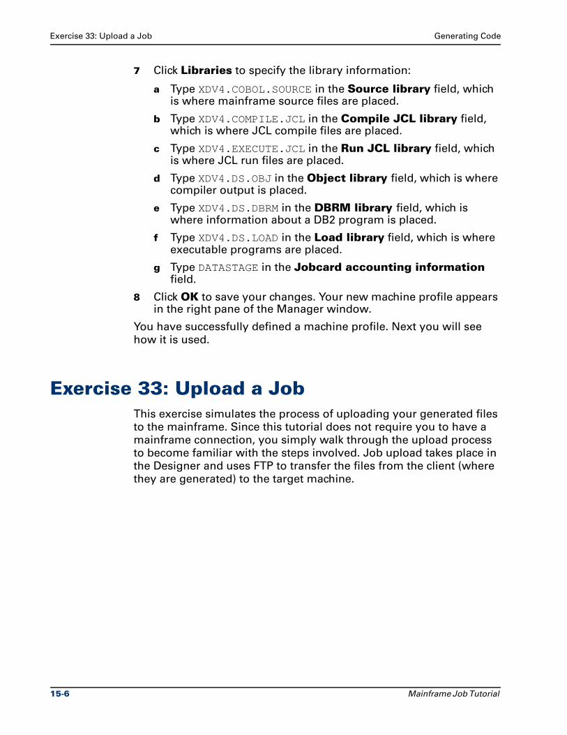
Exercise 33: Upload a Job Generating Code
7 Click Libraries to specify the library information:
a Type XDV4.COBOL.SOURCE in the Source library field, which is where mainframe source files are placed.
b Type XDV4.COMPILE.JCL in the Compile JCL library field, which is where JCL compile files are placed.
c Type XDV4.EXECUTE.JCL in the Run JCL library field, which is where JCL run files are placed.
d Type XDV4.DS.OBJ in the Object library field, which is where compiler output is placed.
e Type XDV4.DS.DBRM in the DBRM library field, which is where information about a DB2 program is placed.
f Type XDV4.DS.LOAD in the Load library field, which is where executable programs are placed.
g Type DATASTAGE in the Jobcard accounting information field.
8 Click OK to save your changes. Your new machine profile appears in the right pane of the Manager window.
You have successfully defined a machine profile. Next you will see
how it is used.
Exercise 33: Upload a JobThis exercise simulates the process of uploading your generated files
to the mainframe. Since this tutorial does not require you to have a
mainframe connection, you simply walk through the upload process
to become familiar with the steps involved. Job upload takes place in
the Designer and uses FTP to transfer the files from the client (where
they are generated) to the target machine.
15-6 Mainframe Job Tutorial
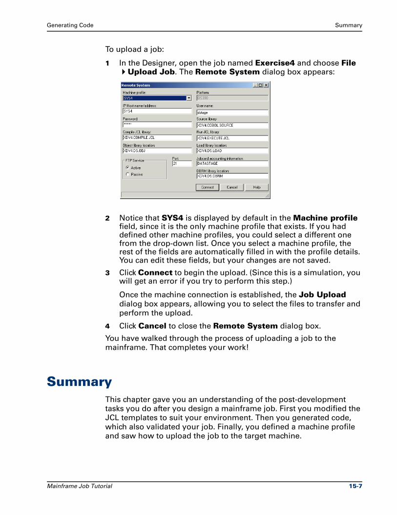
Generating Code Summary
To upload a job:
1 In the Designer, open the job named Exercise4 and choose File Upload Job. The Remote System dialog box appears:
2 Notice that SYS4 is displayed by default in the Machine profile field, since it is the only machine profile that exists. If you had defined other machine profiles, you could select a different one from the drop-down list. Once you select a machine profile, the rest of the fields are automatically filled in with the profile details. You can edit these fields, but your changes are not saved.
3 Click Connect to begin the upload. (Since this is a simulation, you will get an error if you try to perform this step.)
Once the machine connection is established, the Job Upload
dialog box appears, allowing you to select the files to transfer and
perform the upload.
4 Click Cancel to close the Remote System dialog box.
You have walked through the process of uploading a job to the
mainframe. That completes your work!
SummaryThis chapter gave you an understanding of the post-development
tasks you do after you design a mainframe job. First you modified the
JCL templates to suit your environment. Then you generated code,
which also validated your job. Finally, you defined a machine profile
and saw how to upload the job to the target machine.
Mainframe Job Tutorial 15-7
16Summary
This chapter summarizes the main features of Ascential DataStage
Enterprise MVS Edition and recaps what you learned in this tutorial.
Main Features in Ascential DataStage Enterprise MVS Edition
Ascential DataStage Enterprise MVS Edition has the following
features to help you design and build a data warehouse in a
mainframe environment:
Imports meta data from a variety of sources, including COBOL FDs, DB2 DCLGen files, and IMS files. You can view and modify the table definitions at any point during the design of your application. You can also create new table definitions manually.
Reads data from mainframe flat files, including files containing complex data structures and multiple record types. You can set start row and end row parameters, generate an end-of-data row, and pre-sort your source data. You can also choose to normalize or flatten arrays. Constraints allow you to filter data before it is sent to an active stage for processing.
Reads data from IMS databases. You can view the IMS segment hierarchy, define a segment path to read data from, and specify whether to process partial paths or to flatten arrays.
Reads data from mainframe DB2 tables. You can define SQL SELECT statements to extract relational data, including WHERE, GROUP BY, ORDER BY, and HAVING clauses.
Mainframe Job Tutorial 16-1
Recap of the Exercises Summary
Transforms data. A built-in Expression Editor helps you define correct derivation expressions for output columns. A selection of programming components, such as variables, constants, and functions, is available for building expressions. You can also define complex transformations using SQL business rule logic.
Merges data from different sources using joins and lookups. Performs inner, outer, and full joins, as well as singleton and cursor lookups, with a choice of techniques. Also supports conditional lookups, which can improve job performance by skipping a lookup when the data is not needed or is already available.
Aggregates and sorts data.
Combines data from multiple input links into a single output link.
Calls external routines. You can create and save routine definitions for any routine that can be called by a COBOL program, and then incorporate the routines into the generated COBOL programs.
Writes data to flat files and DB2 tables in mainframe environments. An FTP stage allows you to transfer files to another machine.
Reads data from and writes data to external sources and targets. You can write external source and target program in any language callable by COBOL, and create routine definitions that can be called in any mainframe job.
Generates COBOL source, compile JCL, and run JCL files. A set of customizable JCL templates allows you to produce the JCL specific to your job. The COBOL program can also be customized to meet your shop standards.
Traces run-time information about the program and data flow, which is useful for debugging.
Optionally generates an operational meta XML file describing the processing steps of a job, which you can use in MetaStage for process analysis, impact analysis, and data lineage.
Uploads the generated files to the mainframe, where they are compiled and run to build the data warehouse.
Recap of the ExercisesYou learned how to use the Ascential DataStage Enterprise MVS
Edition tool set through a series of exercises involving job design,
meta data management, and project administration.
16-2 Mainframe Job Tutorial
Summary Recap of the Exercises
Although Ascential DataStage Enterprise MVS Edition can support
much more advanced scenarios than appeared in this tutorial, you
gained an understanding of its essential features and capabilities.
The following list describes the functions covered in the exercises:
1 Specifying project defaults and global settings for mainframe jobs.
2 Importing table definitions from mainframe sources.
3 Specifying Designer options applicable to mainframe jobs.
4 Creating, editing, and saving mainframe jobs.
5 Validating jobs and generating code.
6 Creating and editing Transformer stages.
7 Using the Expression Editor:
Defining constraints, stage variables, and job parameters
Creating output column derivation expressions
8 Creating and editing Fixed-Width Flat File source and target stages.
9 Creating and editing Delimited Flat File source and target stages.
10 Creating and editing DB2 Load Ready Flat File stages.
11 Creating and editing FTP stages.
12 Creating and editing Complex Flat File stages.
13 Flattening and normalizing arrays.
14 Working with OCCURS DEPENDING ON clauses.
15 Creating and editing Multi-Format Flat File stages.
16 Importing meta data from IMS sources.
17 Creating and editing IMS stages.
18 Creating and editing Relational source and target stages.
19 Reading data from external sources:
Creating external source routine definitions in the Repository
Creating and editing External Source stages
20 Writing data to external targets:
Creating external target routine definitions in the Repository
Creating and editing External Target stages
21 Merging data using Join stages.
22 Merging data using Lookup stages.
23 Sorting data using Sort stages.
Mainframe Job Tutorial 16-3
Contacting Ascential Software Corporation Summary
24 Sorting data using the source stage pre-sort capability.
25 Aggregating data using Aggregator stages.
26 Aggregating data using the ENDOFDATA variable.
27 Defining SQL business rule logic using Business Rule stages.
28 Calling external routines:
Defining routine meta data in the Repository
Creating and editing External Routine stages
29 Customizing JCL templates.
30 Defining machine profiles in the Repository.
31 Uploading jobs to the mainframe.
During the tutorial you also learned how to navigate the DataStage
user interface in:
The DataStage Manager and Repository
The DataStage Designer
The DataStage Administrator
You worked on some fairly complex examples, but saw how easy it
can be to manipulate data with the right tools.
Contacting Ascential Software CorporationIf you have any questions about Ascential DataStage Enterprise MVS
Edition, or want to speak with someone from Ascential regarding your
particular situation and needs, visit our Web site at http://
www.ascentialsoftware.com or call us at (508) 366-3888.
We will be happy to answer any questions you may have.
We hope you enjoyed working with Ascential DataStage Enterprise
MVS Edition and that this tutorial demonstrated the powerful
capabilities our product provides to help you achieve your data
warehousing goals.
16-4 Mainframe Job Tutorial
ASample Data Definitions
This appendix contains table and column definitions for the data used
in the exercises.
The following tables contain the complete table and column
definitions for the sample data. They illustrate how the properties for
each table should appear when viewed in the Repository.
The COBOL file definitions are listed first, in alphabetical order,
followed by the DB2 DCLGen file definitions and the IMS definitions.
Mainframe Job Tutorial A-1
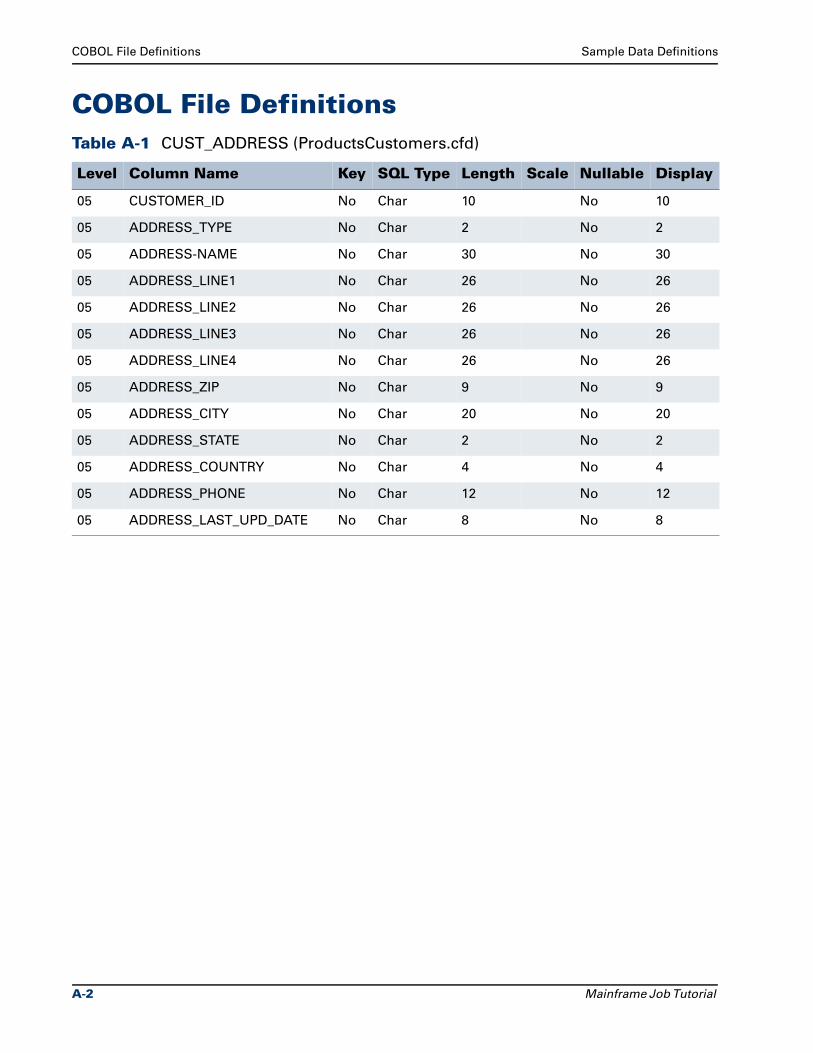
COBOL File Definitions Sample Data Definitions
COBOL File DefinitionsTable A-1 CUST_ADDRESS (ProductsCustomers.cfd)
Level Column Name Key SQL Type Length Scale Nullable Display
05 CUSTOMER_ID No Char 10 No 10
05 ADDRESS_TYPE No Char 2 No 2
05 ADDRESS-NAME No Char 30 No 30
05 ADDRESS_LINE1 No Char 26 No 26
05 ADDRESS_LINE2 No Char 26 No 26
05 ADDRESS_LINE3 No Char 26 No 26
05 ADDRESS_LINE4 No Char 26 No 26
05 ADDRESS_ZIP No Char 9 No 9
05 ADDRESS_CITY No Char 20 No 20
05 ADDRESS_STATE No Char 2 No 2
05 ADDRESS_COUNTRY No Char 4 No 4
05 ADDRESS_PHONE No Char 12 No 12
05 ADDRESS_LAST_UPD_DATE No Char 8 No 8
A-2 Mainframe Job Tutorial
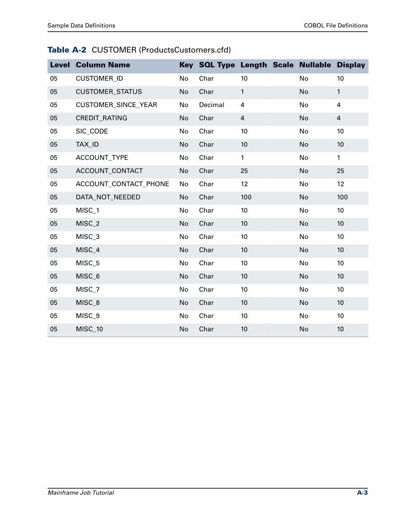
Sample Data Definitions COBOL File Definitions
Table A-2 CUSTOMER (ProductsCustomers.cfd)
Level Column Name Key SQL Type Length Scale Nullable Display
05 CUSTOMER_ID No Char 10 No 10
05 CUSTOMER_STATUS No Char 1 No 1
05 CUSTOMER_SINCE_YEAR No Decimal 4 No 4
05 CREDIT_RATING No Char 4 No 4
05 SIC_CODE No Char 10 No 10
05 TAX_ID No Char 10 No 10
05 ACCOUNT_TYPE No Char 1 No 1
05 ACCOUNT_CONTACT No Char 25 No 25
05 ACCOUNT_CONTACT_PHONE No Char 12 No 12
05 DATA_NOT_NEEDED No Char 100 No 100
05 MISC_1 No Char 10 No 10
05 MISC_2 No Char 10 No 10
05 MISC_3 No Char 10 No 10
05 MISC_4 No Char 10 No 10
05 MISC_5 No Char 10 No 10
05 MISC_6 No Char 10 No 10
05 MISC_7 No Char 10 No 10
05 MISC_8 No Char 10 No 10
05 MISC_9 No Char 10 No 10
05 MISC_10 No Char 10 No 10
Mainframe Job Tutorial A-3
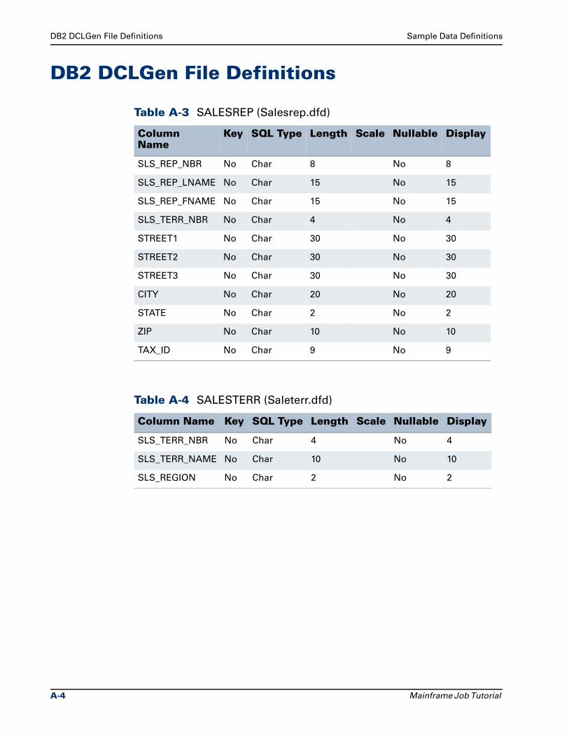
DB2 DCLGen File Definitions Sample Data Definitions
DB2 DCLGen File Definitions
Table A-3 SALESREP (Salesrep.dfd)
ColumnName
Key SQL Type Length Scale Nullable Display
SLS_REP_NBR No Char 8 No 8
SLS_REP_LNAME No Char 15 No 15
SLS_REP_FNAME No Char 15 No 15
SLS_TERR_NBR No Char 4 No 4
STREET1 No Char 30 No 30
STREET2 No Char 30 No 30
STREET3 No Char 30 No 30
CITY No Char 20 No 20
STATE No Char 2 No 2
ZIP No Char 10 No 10
TAX_ID No Char 9 No 9
Table A-4 SALESTERR (Saleterr.dfd)
Column Name Key SQL Type Length Scale Nullable Display
SLS_TERR_NBR No Char 4 No 4
SLS_TERR_NAME No Char 10 No 10
SLS_REGION No Char 2 No 2
A-4 Mainframe Job Tutorial
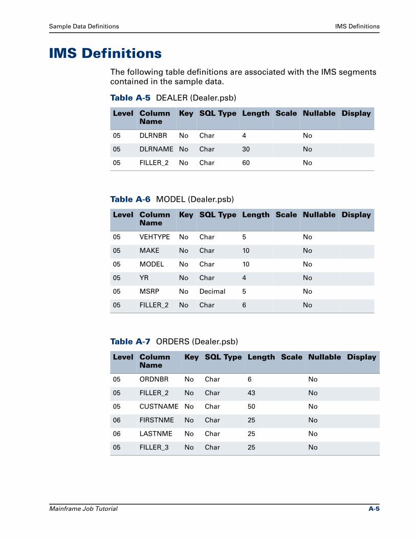
Sample Data Definitions IMS Definitions
IMS DefinitionsThe following table definitions are associated with the IMS segments
contained in the sample data.
Table A-5 DEALER (Dealer.psb)
Level Column Name
Key SQL Type Length Scale Nullable Display
05 DLRNBR No Char 4 No
05 DLRNAME No Char 30 No
05 FILLER_2 No Char 60 No
Table A-6 MODEL (Dealer.psb)
Level ColumnName
Key SQL Type Length Scale Nullable Display
05 VEHTYPE No Char 5 No
05 MAKE No Char 10 No
05 MODEL No Char 10 No
05 YR No Char 4 No
05 MSRP No Decimal 5 No
05 FILLER_2 No Char 6 No
Table A-7 ORDERS (Dealer.psb)
Level ColumnName
Key SQL Type Length Scale Nullable Display
05 ORDNBR No Char 6 No
05 FILLER_2 No Char 43 No
05 CUSTNAME No Char 50 No
06 FIRSTNME No Char 25 No
06 LASTNME No Char 25 No
05 FILLER_3 No Char 25 No
Mainframe Job Tutorial A-5
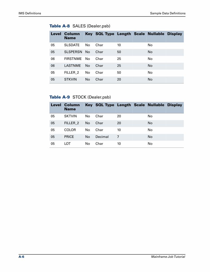
IMS Definitions Sample Data Definitions
Table A-8 SALES (Dealer.psb)
Level ColumnName
Key SQL Type Length Scale Nullable Display
05 SLSDATE No Char 10 No
05 SLSPERSN No Char 50 No
06 FIRSTNME No Char 25 No
06 LASTNME No Char 25 No
05 FILLER_2 No Char 50 No
05 STKVIN No Char 20 No
Table A-9 STOCK (Dealer.psb)
Level ColumnName
Key SQL Type Length Scale Nullable Display
05 SKTVIN No Char 20 No
05 FILLER_2 No Char 20 No
05 COLOR No Char 10 No
05 PRICE No Decimal 7 No
05 LOT No Char 10 No
A-6 Mainframe Job Tutorial
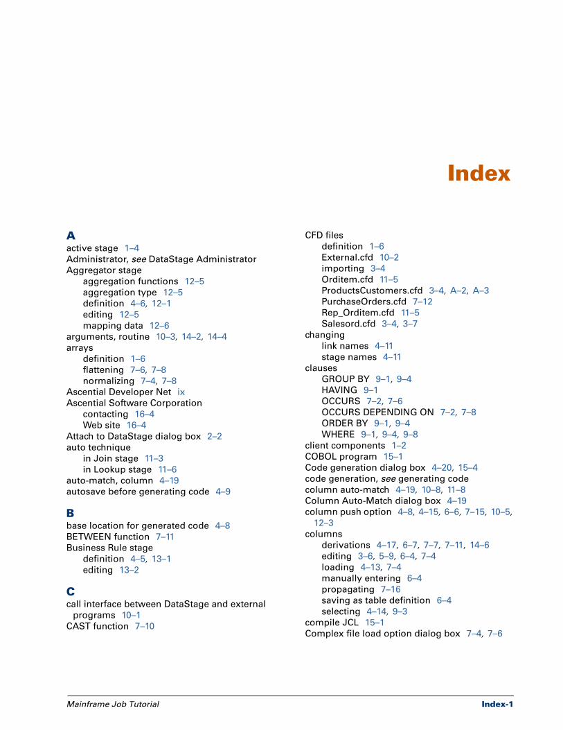
Index
Aactive stage 1–4
Administrator, see DataStage Administrator
Aggregator stage
aggregation functions 12–5
aggregation type 12–5
definition 4–6, 12–1
editing 12–5
mapping data 12–6
arguments, routine 10–3, 14–2, 14–4
arrays
definition 1–6
flattening 7–6, 7–8
normalizing 7–4, 7–8
Ascential Developer Net ix
Ascential Software Corporation
contacting 16–4
Web site 16–4
Attach to DataStage dialog box 2–2
auto technique
in Join stage 11–3
in Lookup stage 11–6
auto-match, column 4–19
autosave before generating code 4–9
Bbase location for generated code 4–8
BETWEEN function 7–11
Business Rule stage
definition 4–5, 13–1
editing 13–2
Ccall interface between DataStage and external
programs 10–1
CAST function 7–10
Mainframe Job Tutorial
CFD files
definition 1–6
External.cfd 10–2
importing 3–4
Orditem.cfd 11–5
ProductsCustomers.cfd 3–4, A–2, A–3
PurchaseOrders.cfd 7–12
Rep_Orditem.cfd 11–5
Salesord.cfd 3–4, 3–7
changing
link names 4–11
stage names 4–11
clauses
GROUP BY 9–1, 9–4
HAVING 9–1
OCCURS 7–2, 7–6
OCCURS DEPENDING ON 7–2, 7–8
ORDER BY 9–1, 9–4
WHERE 9–1, 9–4, 9–8
client components 1–2
COBOL program 15–1
Code generation dialog box 4–20, 15–4
code generation, see generating code
column auto-match 4–19, 10–8, 11–8
Column Auto-Match dialog box 4–19
column push option 4–8, 4–15, 6–6, 7–15, 10–5, 12–3
columns
derivations 4–17, 6–7, 7–7, 7–11, 14–6
editing 3–6, 5–9, 6–4, 7–4
loading 4–13, 7–4
manually entering 6–4
propagating 7–16
saving as table definition 6–4
selecting 4–14, 9–3
compile JCL 15–1
Complex file load option dialog box 7–4, 7–6
Index-1
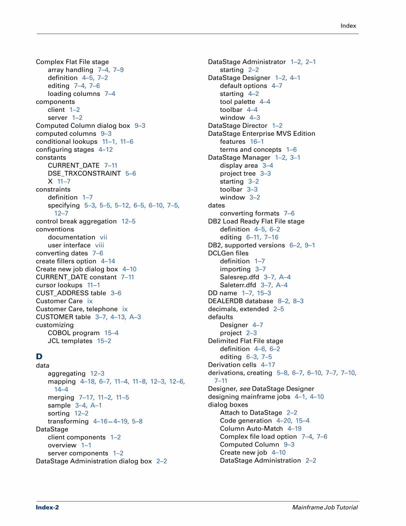
Index
Complex Flat File stage
array handling 7–4, 7–9
definition 4–5, 7–2
editing 7–4, 7–6
loading columns 7–4
components
client 1–2
server 1–2
Computed Column dialog box 9–3
computed columns 9–3
conditional lookups 11–1, 11–6
configuring stages 4–12
constants
CURRENT_DATE 7–11
DSE_TRXCONSTRAINT 5–6
X 11–7
constraints
definition 1–7
specifying 5–3, 5–5, 5–12, 6–5, 6–10, 7–5, 12–7
control break aggregation 12–5
conventions
documentation vii
user interface viii
converting dates 7–6
create fillers option 4–14
Create new job dialog box 4–10
CURRENT_DATE constant 7–11
cursor lookups 11–1
CUST_ADDRESS table 3–6
Customer Care ix
Customer Care, telephone ix
CUSTOMER table 3–7, 4–13, A–3
customizing
COBOL program 15–4
JCL templates 15–2
Ddata
aggregating 12–3
mapping 4–18, 6–7, 11–4, 11–8, 12–3, 12–6, 14–4
merging 7–17, 11–2, 11–5
sample 3–4, A–1
sorting 12–2
transforming 4–16—4–19, 5–8
DataStage
client components 1–2
overview 1–1
server components 1–2
DataStage Administration dialog box 2–2
Index-2
DataStage Administrator 1–2, 2–1
starting 2–2
DataStage Designer 1–2, 4–1
default options 4–7
starting 4–2
tool palette 4–4
toolbar 4–4
window 4–3
DataStage Director 1–2
DataStage Enterprise MVS Edition
features 16–1
terms and concepts 1–6
DataStage Manager 1–2, 3–1
display area 3–4
project tree 3–3
starting 3–2
toolbar 3–3
window 3–2
dates
converting formats 7–6
DB2 Load Ready Flat File stage
definition 4–5, 6–2
editing 6–11, 7–16
DB2, supported versions 6–2, 9–1
DCLGen files
definition 1–7
importing 3–7
Salesrep.dfd 3–7, A–4
Saleterr.dfd 3–7, A–4
DD name 1–7, 15–3
DEALERDB database 8–2, 8–3
decimals, extended 2–5
defaults
Designer 4–7
project 2–3
Delimited Flat File stage
definition 4–6, 6–2
editing 6–3, 7–5
Derivation cells 4–17
derivations, creating 5–8, 6–7, 6–10, 7–7, 7–10, 7–11
Designer, see DataStage Designer
designing mainframe jobs 4–1, 4–10
dialog boxes
Attach to DataStage 2–2
Code generation 4–20, 15–4
Column Auto-Match 4–19
Complex file load option 7–4, 7–6
Computed Column 9–3
Create new job 4–10
DataStage Administration 2–2
Mainframe Job Tutorial
Index
Edit Column Meta Data 3–6
Fixed-Width Flat File Stage 4–13
FTP stage 6–13
Import Meta Data (CFD) 3–5
Import Meta Data (DCLGen) 3–8
JCL Templates 15–2
Job Properties 5–11
Machine Profile 15–5
Mainframe Routine 10–3
Options 4–7
Project Properties 2–4
Remote System 15–7
Save Job As 5–2
Save table definition 6–4
Select Columns 4–14
Table Definition 9–7
Transformer Stage Constraints 5–3
Transformer Stage Properties 5–6, 5–8
DLERPSBR viewset 8–3, 8–5
documentation
conventions vii
DSE_TRXCONSTRAINT constant 5–6
EEdit Column Meta Data dialog box 3–6
editing
Aggregator stage 12–5
Business Rule stage 13–2
columns 3–6, 5–9, 6–4, 7–4
Complex Flat File stage 7–4, 7–6
DB2 Load Ready Flat File stage 6–11, 7–16
Delimited Flat File stage 6–3, 7–5
External Routine stage 14–3
External Source stage 10–5
External Target stage 10–7
Fixed-Width Flat File stage 4–12, 4–15, 5–10, 6–8
FTP stage 6–12
IMS stage 8–6
job properties 5–11, 9–2
Join stage 11–3
Lookup stage 11–6
Multi-Format Flat File stage 7–13
Relational stage 9–3, 9–5
Sort stage 12–2
Transformer stage 4–16, 5–2, 6–7, 7–10, 12–7, 14–5
end-of-data row 6–2, 7–2, 12–1, 12–7
ENDOFDATA variable 12–1, 12–6
exercises
aggregating data 12–3
Mainframe Job Tutorial
calling an external routine 10–5, 10–7, 14–2
controlling relational transactions 13–1
creating a mainframe job 4–9
defining a business rule 13–1
defining a constraint 5–1
defining a job parameter 5–10
defining a machine profile 15–4
defining a stage variable 5–7
defining routine meta data 10–2, 10–6, 14–1
flattening an array 7–6
generating code 4–20, 15–3
importing IMS definitions 8–1
importing table definitions 3–4
CFD files 3–4
DCLGen files 3–7
merging data from multiple record
types 7–17
merging data using a Join stage 11–2
merging data using a Lookup stage 11–5
modifying JCL templates 15–1
overview 1–5
reading data
from a complex flat file 7–3
from a delimited flat file 6–3
from a fixed-width flat file 4–12
from a relational source 9–2
from an external source 10–2
from an IMS file 8–6
recap 16–2
setting project defaults 2–1
sorting data 12–2
specifying Designer options 4–7
uploading a job 15–6
using a Complex Flat File stage 7–3
using a Multi-Format Flat File stage 7–12
using an FTP stage 6–12
using ENDOFDATA 12–6
validating a job 15–3
working with an OCCURS DEPENDING ON
clause 7–8
writing data
to a DB2 load ready flat file 6–9
to a delimited flat file 7–5
to a fixed-width flat file 4–15
to a relational target 9–5
to an external target 10–6
expiration date, for a new data set 6–9
Expression Editor 1–8, 5–3, 5–4, 5–8, 6–7, 7–7, 12–5, 14–6
expressions
constraints 5–3, 5–5, 5–12
Index-3
Index
definition 1–8
derivations 5–8, 6–7, 6–10, 7–7, 7–10, 7–11
entering 5–4
semantic checking 2–5, 5–4, 5–11
syntax checking 5–4
EXT_ORDERS table 10–2, 10–3, 10–6
extended decimals 2–5
External Routine stage
definition 4–6
editing 14–3
mapping data 14–4
mapping routines 14–4
external routines, see routines
External Source stage
array handling 7–9
definition 4–7
editing 10–5
External Target stage
definition 4–6
editing 10–7
FFILLER items 4–14
Fixed-Width Flat File stage
definition 4–6, 6–2
editing 4–12, 4–15, 5–10, 6–8
end-of-data row 12–7
loading columns 4–13
pre-sorting source data 12–4
Fixed-Width Flat File Stage dialog box 4–13
flat file
definition 1–8
stage types 6–1, 7–2
flat file NULL indicators 2–5
flattening arrays 7–6, 7–8
FTP stage
definition 4–6
editing 6–12
FTP Stage dialog box 6–13
full joins 11–1
functions
BETWEEN 7–11
CAST 7–10
IF THEN ELSE 5–9, 6–10, 7–11, 12–8, 14–5
LPAD 6–7
TRIM 7–7
Ggenerating code 4–20, 15–1, 15–3
autosave before 4–9
base location 4–8
Index-4
COBOL program 15–1
compile JCL 15–1
run JCL 15–1
source viewer 4–8
tracing runtime information 15–4
group by aggregation 12–5
GROUP BY clause 9–1, 9–4
Hhash table 1–8
hash technique
in Join stage 11–3
in Lookup stage 11–6
HAVING clause 9–1
hexadecimals 11–7
HTML file, saving as 4–14, 4–20
IIF THEN ELSE function 5–9, 6–10, 7–11, 12–8,
14–5
Import IMS Database (DBD) dialog box 8–2
Import IMS Viewset (PSB/PCB) dialog box 8–3
Import Meta Data (CFD) dialog box 3–5
Import Meta Data (DCLGen) dialog box 3–8
importing
CFD files 3–4
DCLGen files 3–7
IMS files 8–1
IMS Database Editor 8–4
IMS files
Dealer.dbd 8–2
Dealer.psb 8–3, A–5, A–6
IMS stage
definition 4–6
editing 8–6
IMS Viewset Editor 8–5
inner joins 11–1
JJCL
compile 15–1
definition 15–1
for external routines 10–4, 10–5, 10–7
run 15–1
templates 15–1
JCL Templates dialog box 15–2
job control language, see JCL
job parameters
definition 1–9, 5–10
specifying 5–11, 7–3
Mainframe Job Tutorial
Index
Job Properties dialog box 5–11
job properties, editing 5–11, 9–2
jobs, see also mainframe jobs
definition 1–3, 1–9
mainframe 1–4
parallel 1–3
server 1–3
Join stage
definition 4–7, 11–1
editing 11–3
join condition 11–3
join technique 11–3
mapping data 11–4
outer table 11–1
joins
full 11–1
inner 11–1
outer 11–1
Llibraries 15–6
Link Collector stage
definition 4–7
links
area, in Transformer stage 4–17
changing names 4–11
execution order, specifying 5–6
inserting columns into 5–9
marking 4–15
moving 14–3
reference, in Lookup stage 11–5
reject, in Transformer stage 5–5
stream, in Lookup stage 11–5
loading columns
in Complex Flat File stage 7–4
in Fixed-Width Flat File stage 4–13
in Multi-Format Flat File stage 7–13
logon settings 2–2
Lookup stage
definition 4–6, 11–1
editing 11–6
lookup condition 11–8
lookup technique 11–6
pre-lookup condition 11–6
reference link 11–5
stream link 11–5
lookups
conditional 11–1, 11–6
cursor 11–1
singleton 11–1
LPAD function 6–7
Mainframe Job Tutorial
MMachine Profile dialog box 15–5
machine profiles 6–13, 15–4
mainframe jobs
changing link names 4–11
changing stage names 4–11
configuring stages 4–12
definition 1–4
designing 4–1, 4–10
generating code 4–20, 15–3
post-processing stage 1–5
processing stages 1–5
source stages 1–4
target stages 1–4
uploading 15–6
validating 15–3
Mainframe Routine dialog box 10–3
Manager, see DataStage Manager
mapping data
from Aggregator stage 12–6
from External Routine stage 14–4
from Join stage 11–4
from Lookup stage 11–8
from Sort stage 12–3
from Transformer stage 4–18, 5–2, 6–7
markers, link 4–15
MCUST_REC record 7–12, 7–14
merging data
using Join stage 11–2
using Lookup stage 11–5
using Multi-Format Flat File stage 7–17
meta data
area, in Transformer stage 4–17
definition 1–9
editing column 3–6, 5–9, 6–4, 7–4
importing 3–1
routine 10–2, 10–6, 14–1
meta data, operational 2–5, 15–5
MINV_REC record 7–12, 7–14
modifying JCL templates 15–2
MORD_REC record 7–12, 7–14
moving links 14–3
Multi-Format Flat File stage
array handling 7–9
definition 4–6, 7–2
editing 7–13
loading records 7–13
specifying record ID 7–14
Index-5
Index
Nnested technique, in Join stage 11–3
NEWREPS table 9–6, 9–7
normalizing arrays 7–4, 7–8
NULL indicators, flat file 2–5
OOCCURS clause 7–2, 7–6
OCCURS DEPENDING ON clause 7–2, 7–8
operational meta data 2–5, 15–5
Options dialog box 4–7
options, Designer 4–7
ORDER BY clause 9–1, 9–4
ORDER_ITEMS table 11–5
ORDERS table 10–7
OS/390 1–9
outer joins 11–1
outer table, in Join stage 11–1
overview
of Ascential DataStage 1–1
of exercises 1–5
of tutorial iii
Pparallel jobs 1–3
parameters, job 5–11
passive stage 1–4
post-processing stage 1–5
prerequisites, tutorial iv
pre-sorting source data 6–2, 7–2, 12–1, 12–4
processing stages 1–5
PRODUCTS table 3–7, 7–4, 7–6, 7–9
project defaults 2–3
Project Properties dialog box 2–4
project tree 3–3
projects 1–2
propagating columns 7–16
QQSAM 1–10, 7–2
Rrecord ID 7–14
records
loading 7–13
MCUST_REC 7–12, 7–14
MINV_REC 7–12, 7–14
MORD_REC 7–12, 7–14
reference link, in Lookup stage 11–5
reject link, defining 5–5
Index-6
REJECTEDCODE variable 5–5
Relational stage
as source 9–1, 9–2
as target 9–1, 9–5
defining computed columns 9–3
definition 4–6
editing 9–3, 9–5
GROUP BY clause 9–1, 9–4
HAVING clause 9–1
ORDER BY clause 9–1, 9–4
SQL SELECT statement 9–1, 9–4
WHERE clause 9–1, 9–4, 9–8
Remote System dialog box 15–7
REP_ORDER_ITEMS table 11–5, 11–6, 12–2, 12–4
Repository 1–10, 3–1
retention period, for a new data set 6–8
routines
arguments 10–3, 14–2
calling 10–1, 10–5, 14–2
defining the call interface 10–1
definition 1–8
external 14–1
external source 10–2
external target 10–6
mapping arguments 14–4
meta data 10–2, 10–6, 14–1
rows per commit 9–2
RTL, see run-time library
run JCL 15–1
runtime information, tracing 15–4
run-time library 1–10
SSALES_ORDERS table 3–7, 11–3
SALESREP table 3–8, 9–3, 11–2, A–4
SALESTERR table 3–8, 9–3, 11–2
sample data 3–4, A–1
save as HTML file 4–14, 4–20
Save Job As dialog box 5–2
Save table definition dialog box 6–4
Select Columns dialog box 4–14
semantic checking 2–5, 5–4, 5–11
server components 1–2
server jobs 1–3
singleton lookups 11–1
Sort stage
definition 4–7, 12–1
editing 12–2
mapping data 12–3
source stages 1–4
Mainframe Job Tutorial
Index
source viewer 4–8
SQL SELECT statement 9–1, 9–4
SQLCA.SQLCODE variable 13–3
stage variables
derivations 5–8, 6–10, 7–10
specifying 5–7
typical uses 5–7
stages
active 1–4
Aggregator 12–1, 12–5
Business Rule 13–1
changing names 4–11
Complex Flat File 7–2, 7–4
configuring 4–12
DB2 Load Ready Flat File 6–2, 6–11, 7–16
definitions 4–7
Delimited Flat File 6–2, 6–3, 7–5
External Routine 14–3
External Source 10–5
External Target 10–7
Fixed-Width Flat File 4–12, 4–15, 5–10, 6–2, 6–8
FTP 6–12
IMS 8–6
Join 11–1, 11–3
Lookup 11–1, 11–6
Multi-Format Flat File 7–2, 7–12
passive 1–4
post-processing 1–5
processing 1–5
Relational 9–1, 9–3, 9–5
Sort 12–1, 12–2
source 1–4
target 1–4
Transformer 4–16, 5–2, 6–7, 7–10, 12–7, 14–5
STOCK table A–6
stream link, in Lookup stage 11–5
syntax checking 5–4
TTable Definition dialog box 9–7
table definitions
definition 1–10
importing 3–1
loading 4–13, 7–4
manually entering 6–4
saving columns as 6–4
tables
CUST_ADDRESS 3–6
CUSTOMER 3–7, 4–13, A–3
Mainframe Job Tutorial
EXT_ORDERS 10–2, 10–3, 10–6
NEWREPS 9–6, 9–7
ORDER_ITEMS 11–5
ORDERS 10–7
PRODUCTS 3–7, 7–4, 7–6, 7–9
REP_ORDER_ITEMS 11–5, 11–6, 12–2, 12–4
SALES_ORDERS 3–7, 11–3
SALESREP 3–8, 9–3, 11–2, A–4
SALESTERR 3–8, 9–3, 11–2
STOCK A–6
target stages 1–4
technique
join 11–3
lookup 11–6
templates, JCL 15–1
Teradata Export stage 1–10, 4–6
Teradata Load stage 1–10, 4–7
Teradata Relational stage 1–10, 4–7
terms and concepts 1–6
tool palette, Designer 4–4
toolbars
Designer 4–4
Manager 3–3
Transformer Editor 4–18
ToolTips
Designer 4–4
Manager 3–3
Transformer Editor 4–18
tracing runtime information 15–4
transaction control 13–1
Transformer Editor 4–17
column auto-match 4–19
Links area 4–17
Meta Data area 4–17
toolbar 4–18
Transformer stage
definition 4–7
editing 4–16, 5–2, 6–7, 7–10, 12–7, 14–5
link execution order 5–6
mapping data 4–18, 5–2, 6–7
propagating columns 7–16
reject link 5–5
specifying constraints 5–3, 5–12, 12–7
specifying derivations 6–7, 7–7, 7–11
specifying stage variables 5–7, 7–10
Transformer Stage Constraints dialog box 5–3
Transformer Stage Properties dialog box 5–6, 5–8
transforming data 4–16—4–19, 5–8
TRIM function 7–7
Index-7
Index
tutorial
getting started 1–5
overview iii
prerequisites iv
recap 16–2
sample data 3–4
two file match technique, in Join stage 11–3
Uuploading jobs 15–6
user interface conventions viii
Vvalidating jobs 15–3
variables
ENDOFDATA 12–1, 12–6
REJECTEDCODE 5–5
SQLCA.SQLCODE 13–3
VSAM 1–11, 7–2
WWHERE clause 9–1, 9–4, 9–8
windows
DataStage Designer 4–3
DataStage Manager 3–2
XX constant 11–7
Index-8
Mainframe Job Tutorial