ANALYSIS OF MULTI-COLUMN PIER OF UNSKEWED BRIDGE USING STAAD.Pro UNDER

STATIC AND DYNAMIC LOAD

Othman, N.S.U

Researcher, Faculty of Civil Engineering, Universiti Teknologi MARA, 40450 Shah Alam, Selangor D.E

ABSTRACT

Bridges in Malaysia are usually design under static loading. Some major cities in Malaysia had experienced earthquake excitation or ground motion upon devastating Tsunami and Earthquake event held in Acheh back in 2004. Performing simple harmonic motion analysis for the single degree of freedom (SDOF) bridge structure under free vibration without damping using STAAD Pro was a new adaptive study. The model of the bridge had been modified in specifications (from existing bridge in Jeli, Kelantan) suitably for dynamic analysis assignment. Commenced with the validation of the static loading for the modified prototype bridge pier structure using mathematical calculation, the comparison shown between analytical and theoretical was almost 0%. Thus in dynamic analysis, two parameters were verified and validated using theories and calculation, which are maximum lateral displacement and Rayleigh frequency under 6 various percentage of drift. Numerical results indicate excellent accuracy when the percentage difference between analytical and numerical for maximum lateral displacement and Rayleigh frequency was only 4.705% and 2.18%, respectively. It designates a good accuracy and acceptable to be used and compared in laboratory experiment of the same specimen for continuity of the study. Both static and dynamic analysis were successfully verified and validated. In supplementary, the free vibration without damping system analysis produces more information and relevant data’s that merely could be used in researching the performance of the bridge structure under dynamic responses.

Keywords: multi-column pier bridge, unskewed bridge, STAAD Pro dynamic analysis, bridge analysis, concrete bridge, dynamic loading, time history analysis, simple harmonic motion, free vibration without damp.

1.0 INTRODUCTION

The huge earthquake excitation from neighboring, such as Banda Acheh, Sumatera could feel in Malaysia due to long distant earthquakes can cause damage to buildings and bridges. Second Penang Bridge which connecting Batu Kawan in mainland and Batu Maung in the Island with span about 24km across the sea is the longest seismic design bridge in the world (Time, 2012). Most of the mega project of bridges in Malaysia has induced the seismic loading into their design calculation, but what about the bridge that was constructed earlier in accordance to British Standard (BS8110). Modeling of the prototype building is the best approach to be conducted using the existing bridge or even to every new design of bridges in a future. The main focus of this study is to look into the bridge bents and allowable displacements. How it moves and displaced during earthquake event should be investigated. The ability of design and use structural software to model the sub-assemblage of bridge pier under earthquake loading is important examine the seismic performance. Though seismic analyses can be done using modeling method for bridges are not much compared to buildings, the end results obtained showed that bridges behave in an interesting way that illustrates the mode of shape and damages of the bridge undergone some deformation.

This study is taking a wise step in conducting modeling analysis using STAAD.Pro to a modified prototype of multi-column pier of unskewed bridge under static and dynamic load. The modification was made to the length, width, type of beam and number of columns at pier from the original bridge. An analysis of undamped free-vibration was applied to the model as the model was constructed and defined as single degree of freedom (SDOF). The intended objective needed to be achieved are (i) to model the modified bridge pier using STAAD Pro, (ii) to perform static and dynamic analysis using STAAD Pro and (iii) to validate each analysis between mathematical modeling and numerical calculation. The dimension of the modified prototype of bridge pier in cross sectional view is as shown in Figure 1.1 and the model properties are as shown in Table 1.1. It is to deliver a performance result of the pier, such as the lateral displacements of the bridge deck. The validation value of static and dynamic (seismic analysis) between analytical modeling and theoretically were obtained and discussed.

Figure 1.1: Cross sectional view of the bridge model

Table 1.1: Modified bridge prototype material properties

ItemDimension

Unit Weight (kN/m3)Thickness

(mm)Length (mm)

Cross Section Area (m2)

Premix 60 - - 23.5

In-situ Slab 160 - - 25

I18 Precast Beam

- 18800 0.598475 25

Parapet - 18800 0.185 25

Capping Beam

1600 9500 2.4 25

Diaphragm 300 - 1.237 25

In-situ Column

1000 5750 0.785 25

2.0 Previous Researchers Work

THA has been used widely to study the performance and the behavior of a structure under earthquake loading. In this study, the Time History Analysis was done by defining the acceleration with time function. 6 pre-determined bridge drift were calculated in order to obtain the amplitude, (A) of the function. Different software might have different interface in data input, moreover the concept remain similar. In most of the THA done to structures, especially bridges, SAP2000 frequently used software, instead of STAAD.Pro. In this study, STAAD.pro was used in conducting Free Vibration of undamped structure for multi-column pier of unskewed bridge. Though, previous researchers had done several works on bridge analysis under dynamic loading with various types of software and approach and also the purposes.

2.1 Dynamic Analysis on Skew Bridge

The direction of the bridge with the underneath traffic flow or river flow or even railway path is divided into two, whether it is skew (not perpendicular to the underneath flow) or unskewed (perpendicular or parallel to the underneath direction. Several studies had been performed for skew bridge under dynamic impact or loads. The bridge over the Yarriambiack Creek at Warracknabeal Victoria in Australia was tested under dynamic loading both in computer modeling and experimentally with 30 of skew angle (Haritos, 1995). The shaker (the actuator) for creating dynamic motion was positioned at two salient points on the bridge model (point A and point B) as shown in Figure 2.1.

Figure 2.1: The plan view of Yarriambiack Creek Bridge test span depicting accelerometer grid (Haritos, 1995).

The model is tested using sweptSine Wave (SSW) displacement/forcing function with range of frequency between 0.5 to 50Hz with maximum double amplitude of 80kN excitation. The comparison between experiementally and numerically were made for the natural frquencies of the model for both position A and B. It was came out acceptable between numerical and experimental results as closed as 5% in the percentage difference. Hence, results from experiment depicted that the optimal model fitting was done between the range of 10Hz to 30Hz as it was already classified as outside of the range. Unlimited from numerical results shows that all 6 modes of the model’s natural frequencies can be printed out.

It is rare to find a great condition of bridge construction in avoiding skew of the bridge. The skew angle could leads to financial support to the whole bridge project. Most of the time, to get unskewed bridge is almost possible. But, the skew angle can actually lessen down the moment of the bridge pier and also the moments and displacement at the center span section (He, 2012). The multi-span box girder bridge was analyzed under static loading with varies of skew angle being assigned to the bridge model. The mode shapes for three type of bearing which are orthogonal double bearing (ODB),

skewed bearing (SB) and orthogonal single bearing (OSB) are shown in Figure 2.2. it shows that different skews and support conditins gives minimal effect on the first mode shape of the model bridge. Increasing skew apparently increasing the first modal frequency. Increasing skew was observed to increase the modal frequencies but no obvious trend for higher modes. It is appears that with increasing of skew angle it increases the apparent stiffness relative to mass.

Figure 2.2: Calculated mode shapes comparison of orthogonal double bearing (ODB), skewed bearing (SB) and orthogonal single bearing (OSB) (He, 2012).

2.2 Dynamic Analysis on shape of the bridge deck

The shape of the bridge deck reacts differently when assigned to dynamic loading. Three different span of multi-span concrete bridge was tested using finite element method (FEM). The selected spans were 16-32-16 (64m), 20-32-20 (72m) and 20-40-20 (80m) (Munirudrappa, 2004). The cross section of the studied bridge were Tee section, I section and Box section with the option under skew angle of 0 and 30. In order to obtain the frequencies at different nodes positions, considered speed is in the range of 30kmph, 45kmph, 60kmph, 90kmph to 120kmph. A Laplace transform solution was performed for dynamic load factor (DLF). The observation is discussed and obviously, with the increase of speed and span, the DLF also increase, while respond to the various section of the bridge, they were no appreciable changes. The DLF values also has no significant effect with the skew angle of the bridge (0 and 30, respectively). From the free vibration of the bridge in fundamental mode, the largest dynamic load factor (DLF) occurred at center of the mid span as shown in Figure 2.3.

Figure 2.3: Free Vibration of the bridge in fundamental mode (Munirudrappa, 2004).

Another test was done using finite element method (FEM) in 2 and 3-dimensional of multi-span segmental bridge, Sultan Azlan Shah Bridge in Perak (Azlan et al, 2008). SAP2000 was utilized in modelling and analysing the seismic response to the bridge. Figure 2.4 and Figure 2.5 respectively shows the two dimensional of the bridge simulation and the mode shape of the bridge in longitudinal view. Figure 2.6 and Figure 2.7 respectively shows the three-dimensional of the bridge simulation and the mode shape. Both two and three-dimensional simulation were analysed under Time History Analysis.

Figure 2.4: 2D Computer simulation of the bridge (Azlan et al, 2008).

Figure 2.5: Mode shape 1 of the bridge (Azlan et al, 2008).

Figure 2.6: 3D Computer simulation of the bridge (Azlan et al, 2008).

Figure 2.7: Mode shape in 3D (Azlan et al, 2008).

According to the final comparison, the bridge deck and pier either in 2D or 3D, shows less than the capacity under Time History Analysis. However, the pier of the bridge under 3D response spectrum analyses showed that the value of maximum axial force and maximum bending moment was higher than the capcity when it was subjected to Peak Surface Acceleration (PSA) of 0.161g. The bridge was tested untill it cracks at 0.25g and collapse at 0.32g.

2.3 Free Vibration without damping

The earthquake excitation and bridge responses is subjected to earthquake ground motion in the form of ground acceleration or Peak Ground Acceleration, (PGA), denoted as Üg(t) is best explained as Single Degree of Freedom (SDOF) model of a bridge structure. Figure 2.8 shows part of the longitudinal section of unskewed bridge. A simplified SDOF model of a single column bent bridge under transverse earthquake ground acceleration input can provide similarity or approximation to the true seismic response of the bridge prototype as long as the bridge is unskewed and having constant span and equal heights of piers (Priestly,2009). Figure 2.9 shows the cross sectional of the bridge and

the hatching area show the simplified model that will be analyzed as single degree of freedom (SDOF).

Figure 2.8: Longitudinal section of unskewed bridge (Priestley, 1996)

Figure 2.9: Sub-assemblage of unskewed bridge is modeled as single degree of freedom (SDOF) (Priestley, 1996)

The first mode of vibration characteristics can easily be found as shown in Figure 2.9, where the lumped mass and the stiffness of the column can be selected based on the cross section. From Newton’s Second Law, the undamped-free vibration bridge model can be expressed as

m u( t )+c u ( t )+ku( t )=0 Equation 2.1

m u( t )+ku( t )=0 Equation 2.2

where;

mü = Inertial Forces

cuI = Damping forces

ku = Elastic forces

The displacement u (t) with time is assumed to follow a harmonic motion as shown in Figure 2.10, giving the form

u( t )=A sin(ϖt ) Equation 2.3

(a) Full scale of unskewed bridge (b) Single degree of freedom (SDOF)

As the derivation can be continued to determine the velocity, û(t) with time and acceleration, ü(t), respectively,

u( t )=ϖA cos( ϖt ) Equation 2.4

u( t )=−ϖ2 A sin( ϖt ) Equation 2.5

And for SDOF (single-degree-of-freedom) of bridges consisting undamped natural angular frequency (), the cyclic natural frequency (f) and natural period of vibration (T) can best be defined as

frequency , f = ω2 π Equation 2.6

period ,T=1f=2π

ω Equation 2.7

Figure 2.10: Free vibration for undamped harmonic response of SDOF system.

3.0 MATERIAL AND METHODOLOGY

3.1 Static modeling and analysis

In static modeling and analysis using STAAD Pro, the material properties of the modified prototype bridge are as shown in Table 1.1. The concrete compressive strength is 40N/mm2 and Young’s Modulus of 35000 N/mm2. The dead loads for the analysis were from the selfweight of the beams, diaphragms, parapets, premixes and concrete slab. The general dimension of the bridge model is 18m (length) x9.5m (width) x6.5m (height to the center of the capping beam). In STAAD Pro, the modified prototype bridge is modeled as skeletal statically determinate structure, comprises 3 member elements and 4 nodes. Node 2 and 3 was assigned as a support and design loads were assigned along the member element with appropriate distance (according to the I18 beam position on capping beam) as shown in Figure 3.1. The analytical result was then validated to mathematical calculation.

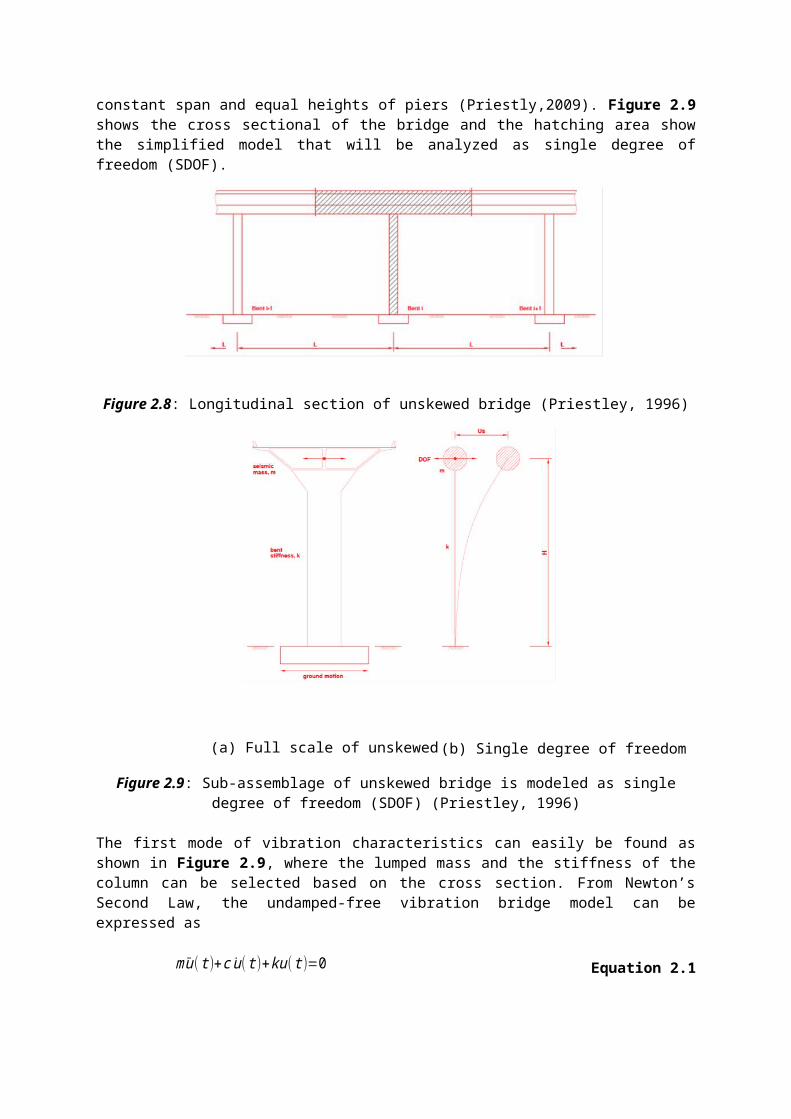
Figure 3.1: Node numbers, member numbers, supports and loading distribution.

3.2 Dynamic modeling and analysis

Simple harmonic motion (SHM) of single degree of freedom (SDOF) of the modified prototype bridge was also modeled using STAAD Pro. The modeling construction was done as skeletal structure (framing structure) with 6 nodes and 5 member elements. Node 5 and node 6 were assigned as fixed support at the column, member 4 and member 5 were assigned as the pier column (1000mm diameter, 6.5m high) and member 1,2 and 3 were assigned as the capping beam (1.5m high x 1.6m depth x 9.5m length). The concentrated lumped mass was position on top of the model (automatically centralized by STAAD Pro system) and expressed as SELFWEIGHT (in both direction, x and y-axis) of the bridge pier. In order to fulfill the simple harmonic motion (SHM) motion of equation, the stiffness

(k )of the column was required. A pre-determined drifts value in percentage varies from 0.01%, 0.1%, 0.25%, 0.5%, and 0.75% to 1% applied to the time-displacement and time-acceleration sine function.

A simple harmonic motion is introduced to the model analysis which intended to obtain the time-displacement function of the model. The maximum displacements of the top column of the model under the time history load case are also obtained. The second derivation of displacement vs. time

following the harmonic motion,u( t )=−ϖ2 A( sin ϖt ) the acceleration amplitude is calculated according to the 6 conditions of drifts. The displacement amplitude (A) is pre-calculated according to the 6 conditions of drifts. The acceleration vs. time function is plotted for each and every drift’s value and tabulated for 6 conditions of period (T) and frequency (f). The angular frequency, () is determined by the stiffness of the columns, (k) and the total mass of the skeletal structure (m).

3.2.1 Acceleration versus Time Function in STAAD Pro

Translational acceleration load are used to simulate the ground motion of the time history analysis acceleration record in STAAD Pro. STAAD Pro software assumes complete fixity to all supports (since the modified prototype bridge pier model are constructed as monolithic structure). Then STAAD Pro automatically computed the acceleration loads at each nodes and structural model. During analysis, acceleration couples with mass and STAAD Pro has distributed the mass of the model to all joints. For this model, Node 1, 2, 3 and 4 are having similar distributed mass and they will be no mass distribution for joints or nodes that has been assigned as supports.

Each and every set of the single degree of freedom (SDOF) analysis, acceleration vs. time function is

plotted using the function ofu( t )=−ϖ2 A( sin ϖt ) . The tabulated data of time (s) and acceleration amplitude (mm/sec2) is plotted using Microsoft Excel and a sine wave curve is drawn. The drawn curve from Microsoft Excel is considered as a theoretical results and the tabulated data is then used as an input data of STAAD Pro Time History – Acceleration Function command.

3.2.2 Displacement versus Time Function in STAAD Pro

Time-Displacement function which resulted to the maximum displacement of the modified prototype bridge pier model is obtained upon the STAAD Pro time history-acceleration loads analysis for single degree of freedom (SDOF) system. The result retrieved from STAAD Pro postprocessing mode was as graphic mode (the displacement vs. time curve).

3.2.3 Supplementary Results from Dynamic Analysis

Apart from the validation of the lateral displacement of the model, verification and validation of the Rayleigh frequency of the model were calculated as well. The equation for calculating Rayleigh frequency is depending on the lateral displacement of the model, the magnitude of the horizontal force (by means the weight of the skeletal structure applied in horizontal direction, which is the SELFWEIGHT in x-direction) and the mass of the skeletal model. Rayleigh frequency (which units in cycle per second, cps) produced from STAAD Pro were then validated by the mathematical calculation of equation as follow

Rayleigh Frequency, Equation 3.1

where;W = Weight of the skeletal structure (kN)M = Mass of the skeletal structure (kg)

4.0 RESULTS AND DISCUSSION

Both static and dynamic analysis results were validated and verified using mathematical solution. The difference percentages were calculated and the difference value has been set limited to below 5% and concluded as verified and acceptable.

4.1 Static analysis result and discussion

For static analysis, the result of bending moment, BM (kN-m), shear force, V (kN) and reaction at supports, R (kN) were summarized, compared between analytical (STAAD pro) and mathematical. The difference percentage for bending moment, BM and shear force, V and support at reactions, R, are as shown in Table 4.1 and Table 4.2, respectively.

Table 4.1: Percentage difference between analytical and theoretical results for bending moment and shear force

Beam

Analytical (STAAD

Pro)

Theoretical (Manual

Calc.)

Bending Moment

Percentage Difference

(%)

Node

Analytical (STAAD

Pro)

Theoretical (Manual

Calc.)

Shear Force

Percentage Difference

(%)Moment (kN-m)

Moment (kN-m)

Shear Force(kN)

Shear Force(kN)

3 504.56 504.56 0 3 630.142 630.1415 0

2 504.56 504.56 0 2 577.598 577.598 0

2 -349.676 -349.677 0.003

3 0 0 0 4 0 0 0

1 0 0 0 1 0 0 0

1 -504.56 -504.56 0 2 630.142 630.1415 0

2

1

22

1

x

x

M

W

2 -504.56 -504.56 0 3 577.598 577.598 0

Table 4.2: Percentage difference between analytical and theoretical results for support reaction

Node

Analytical (STAAD Pro)

Theoretical (Manual Calc.) Percentage

Difference (%)Reaction

(kN)Reaction

(kN)3 1207.74 1207.74 0

2 1207.74 1207.74 0

1 1207.74 1207.74 0

2 1207.74 1207.74 0

The comparison between analytical (STAAD Pro) and theoretical verification were done for the static analysis. The validation was made for STAAD pro with the manual calculation. Theoretically, the value obtained for manual calculation did not show a huge different than the value STAAD Pro had produced. Discussing Table 4.1 and Table 4.2 summarized that values for bending moment, shear force and reaction at supports exhibit almost no differences between analytical and theoretical calculation. Therefore, the manual calculation procedure is correctly performed.

Hereafter, the static analysis of the modified prototype of bridge pier was announced validated theoretically and the results are acceptable. Then, STAAD Pro is satisfied to be used to prolong the study of the dynamic analysis.

4.2 Dynamic analysis result and discussion

4.1 Time-displacement and Rayleigh Frequencies

For simple harmonic motion (SHM) to be done in STAAD Pro, acceleration amplitude was needed in time history fundamental command. The main parameters obtained are the maximum lateral displacement and the time-displacement curve of the modified prototype bridge pier model (a skeletal structure). Nonetheless, STAAD Pro has produced other interesting results which can be discussed further in this chapter. The additional results are the mode shapes of the model, modal frequency, mass participation Rayleigh frequency, maximum base shear at times and peak ground acceleration (PGA) extruded from time-acceleration relationships. The modified prototype bridge pier model, validation and verification is made for the maximum lateral displacement and the Rayleigh frequency of the model. The best presentation of the validation comparison can be shown through Table 4.1 and summarized into the percentage differences between the analytical and theoretical dynamic results.

Both analyses shows that with the increment of drift percentage value, the maximum lateral displacement of the model is also increase. The increment of the lateral displacement is supported by the increment of the time (starting from 60s to 210s) for the model to be analyzed. Initially at the drift of only 0.01%, the maximum lateral displacement produced by STAAD Pro is only 0.6195mm and Microsoft Excel with 0.65mm. When the drift percentage is at 1%, the maximum lateral displacement from STAAD Pro is 61.9531mm lesser 3.0469mm from Microsoft Excel output at 65.00mm. The huge increment in lateral displacement occurred from 0.01% to 1% of drift, which is 61.3336mm for STAAD Pro and 64.35mm for Microsoft Excel. Hence, the average percentage differences between STAAD Pro and Microsoft Excel shown in Table 4.1 are only 4.705%. Therefore, time-displacement relationships produced by Microsoft Excel are considered acceptable since the average percentage difference is less than 5%. The differences occurred in such a way due to both medium capability in processing dynamic data’s into graphical output and result for dynamic analysis.

Additional validations output from STAAD Pro, which was Rayleigh frequency for each and every maximum lateral displacement obtained. The Rayleigh frequencies obtained from STAAD Pro were not constantly increasing in value with the increment of time. Rayleigh frequency is depending much in the lateral displacement value as the weight (W) and mass (m) of the structure are constants. The result shows that at the lowest maximum lateral displacement of the model which denoted by drift 0.01%, the Rayleigh frequency is the highest among others, which are 19.98345Hz from STAAD Pro and 19.54939Hz from theoretical calculation. The Rayleigh frequency values keep fluctuated between drift 0.1% to 0.75% and ended up with the lowest Rayleigh frequency value at drift 1% for 1.99835Hz from STAAD Pro and 1.954939Hz from theoretical calculation. The drop of Rayleigh frequency from drift 0.01% to 1% is almost 10%. Percentage difference between analytical (STAAD Pro) and theoretical results were also presented. The difference made was much lesser than the comparison done to maximum lateral displacement of the model. For Rayleigh frequency average percentage difference is only 2.18%, which is far lesser than the set limit of 5% to make the results acceptable. The theoretical formula used can be said as verified and validated.

Table 4.1: Result comparison and percentage differences between analytical and theoretical analysis of the model

Drift

(%)Description

STAAD Pro

Output

Manual

Calculation

Total Time,

T

(s)

Percentage

Differences

(%)

0.01

Max

imu

m L

ater

al

Dis

pla

cem

ent

(mm

)

0.6195 0.6560 4.69

0.106.1953 6.5

90 4.69

0.2515.4852 16.25

120 4.71

0.5030.964 32.5

150 4.73

0.7546.450 48.75

180 4.72

1.0061.9531 65

210 4.69

0.01

Ray

leig

h F

req

uen

cy

(cyc

le p

er s

econ

d, c

ps)

19.9834519.54939

60 2.17

0.10 6.319326.182061

90 2.17

0.25 3.997093.909878

120 2.18

0.50 2.826662.764702

150 2.19

0.75 2.307932.257369

180 2.19

1.00 1.998351.954939

210 2.17

The time-displacement relationships verified by Microsoft Excel as the requirement of this study for mathematical comparison are shown in Figure 4.1.

Figure 4.1: Time-Displacement Curve for all 6 Drifts of the Modified Prototype Bridge pier model (from Microsoft Excel (Spreadsheet))

4.2 Maximum base shear, Mode shape and modal frequencies of the model

Table 4.2: Maximum base shear, mode shape and modal frequencies for dynamic analysis produced by STAAD Pro

Drift

(%)

Maximum

Base Shear

(kN)

Maximum Base

Shear Time

(s)

Mode 1 Frequency

(Hz)

Mode 2 Frequency

(Hz)

Mass Participation at

Node 1, Mode 1

(%)

0.01 82.59 7.033 6.891 149.444 100

0.10 825.92 7.0336.891 149.444

100

(a) Max. Displacement 0.65mm (b) Max. Displacement 6.5mm

(c) Max. Displacement 6.25mm (d) Max. Displacement 32.50mm

(e) Max. Displacement 48.75mm (f) Max. Displacement 65mm

0.25 2064.40 81.0336.891 149.444

100

0.50 4127.94 81.0296.891 149.444

100

0.75 6192.05 22.0296.891 149.444

100

1.00 8259.24 7.0336.891 149.444

100

The increment of drift percentage and time, the maximum base shears are also increase. Though the time recorded for the maximum base shear (the maximum capacity of the model to withstand the dynamic motion in particular times based on peak ground acceleration (PGA)) is varies. The first two drifts percentage which is 0.01% and 0.1%, the maximum base shear value are ten times higher but the time recorded the same, which is 82.59kN (at 7.033s) and 825.92kN (at 7.033s), respectively. But starting from the third drift percentage of 0.25% to 1%, the maximum base shear is keep increasing from 2064.399kN (at 81.029s) to 8259.241kN (at 7.033s).

STAAD Pro mode shape results produces two types of mode shape, which are mode shape 1 (normal mode shape) and mode shape 2 (torsional mode shape). Figure 4.2 shows the normal mode shape which the shape reflecting the usual lateral displacement of a model. Figure 4.3 shows the torsional mode shape which the movement of the model of the bridge pier is like in twisting motion (torsion) due to the torsional ground motion effect.

5.0 CONCLUSION AND RECOMMENDATION

It has been demonstrated and performed that both static and analysis of the multi-column pier of unskewed bridge using STAAD Pro were verified and satisfactory validated by concept of theories. The maximum lateral displacements and Rayleigh frequency of the modified prototype bridge pier model was studied on various percentages of drift and analytical result was validated by manual calculation. Model analyzed under free vibration without damping system shows that with the increasing of drift percentage, the maximum lateral displacement is also increase. On the other hand with the increment of drift percentage (corresponding to increasing of maximum lateral displacement), the Rayleigh frequency is dropped. The increasing of maximum lateral displacement and decreasing of Rayleigh frequency were due to the collective time assigned to the model. Overall, the results and comparisons obtained were acceptable and utilization of STAAD Pro is appropriate.

This study was only done in 2D analysis using STAAD Pro (as STAAD Pro is infamous finite element analysis software (FEM) compared to ANSYS, CIS, RUAMOKO, SAP2000 and more), yet has the great potential to prolong the study by performing 3D analysis using similar software and setting up laboratory experiment. Therefore, result from this study can be made as a comparison and

Mode Shape 1Load 1 : X

Y

Z

Figure 4.2: Mode shape 1, Frequency 6.891Hz (Normal Mode Shape)

Mode Shape 2Load 1 : X

Y

Z

Figure 4.3: Mode shape 2, Frequency 149.444Hz (Torsional Mode Shape)

input data to the laboratory works and search for the best performance of the bridge model under dynamic loading.

References

Bridge Structural Elements Diagram. (2001). Retrieved Dec Friday, 2013, from Department of Transportation MDOT: www.michigan.gov/mdot

Clarke, R. (2003). STAAD Basics, Notes on the Effective Use of STAAD Pro Rel. 3.1.

Gizem Sevgili and Alp Caner, P. (2009). Improved Seismic Response of Multisimple Span Skewed Bridges Retrofitted with Link Slabs. Journal of Bridge Engineering ASCE, 452-459.

N.Haritos, H. a. (1995). Modal Testing of a Skew Reinforced Concrete Bridge. Department of Civil and Environmental Engineering, The University of Melbourne, Australia, 703-708.

N.Munirudrappa, N. K. (2004). Response of Slant Legged Skew Bridge Under Dynamic Loading. 13th World Conference on Earthquake Engineering, (p. Paper No:3151). Vancouver, B.C, Canada.

Priestley, M. (1996). Seismic Design and Retrofit of Bridges. California, San Diego, USA: John Wiley & Sons, Inc.

Wikipedia. (2013, December 16). Peak Ground Acceleration.

X.H.He, X. A. (2012). Skewed Concrete Box Girder static and dynamic testing and analysis . Elsevier.