Embed Size (px)
Citation preview

MAGNETOUR: Surfing Planetary Systems on Electromagnetic and Multi-Body Gravity Fields
NIAC Phase 1 Final Report July 2013
Gregory Lantoine1, Rodney L. Anderson1, Henry B. Garrett1, Ira Katz1, Damon Landau1, Ryan P. Russell2, Nathan J. Strange1
1 Jet Propulsion Laboratory – California Institute of Technology, Pasadena, CA 91109 2 University of Texas at Austin, Austin, TX 78759
FINAL REPORT NASA INNOVATIVE ADVANCED CONCEPTS (NIAC) PHASE ONE MAGNETOUR: SURFING PLANETARY SYSTEMS ON ELECTROMAGNETIC AND MULTI-BODY GRAVITY FIELDS
MAGNETOUR: Surfing Planetary Systems on Electromagnetic and Multi-Body Gravity Fields
NIAC Phase 1 Final Report July 2013
Principal Investigator: Gregory Lantoine JPL Mission Design & Navigation Section (392) (Point of Contact: [email protected] / 818.354.6640)
Co-Investigators: Rodney L. Anderson JPL Mission Design & Navigation Section (392)
Henry B. Garrett JPL Reliability Engineering & Mission Environmental Assurance Section (513)
Ira Katz JPL Electric Propulsion Group Supervisor (353B)
Damon Landau JPL Mission Design & Navigation Section (392)
Ryan P. Russell The University of Texas at Austin, Assistant Professor
Nathan J. Strange JPL Mission Systems Concepts Section (312)
Consultant: Daniel Grebow JPL Mission Design & Navigation Section (392)

FINAL REPORT NASA INNOVATIVE ADVANCED CONCEPTS (NIAC) PHASE ONE MAGNETOUR: SURFING PLANETARY SYSTEMS ON ELECTROMAGNETIC AND MULTI-BODY GRAVITY FIELDS
Acknowledgements
Part of the research was carried out at the Jet Propulsion Laboratory, California Institute of Technology, under a contract with the National Aeronautics and Space Administration.
We would like to thank Raul Polit Casillas for his involvement in the design of the spacecraft configuration. We would also like to thank Marco Quadrelli for interesting discussions about tether dynamics.
© Copyright 2013. All rights reserved.
ii
FINAL REPORT NASA INNOVATIVE ADVANCED CONCEPTS (NIAC) PHASE ONE MAGNETOUR: SURFING PLANETARY SYSTEMS ON ELECTROMAGNETIC AND MULTI-BODY GRAVITY FIELDS
Contents 1 INTRODUCTION....................................................................................................................5
2 MAGNETOUR CONCEPT .....................................................................................................7
3 PHASE ONE METHODOLOGY & MAIN FINDINGS.........................................................9 3.1 Study Approach ..........................................................................................................9
3.2 Phase One Key Points...............................................................................................10
3.3 Assessment against Phase One Work Plan ...............................................................13
4 OUTER PLANET ENVIRONMENTS..................................................................................14 4.1 Overview...................................................................................................................14
4.2 Radiation Belts..........................................................................................................17
4.2.1 Jupiter radiation belts ...................................................................................17
4.2.2 Saturn radiation belts....................................................................................18
4.2.3 Uranus radiation belts...................................................................................19
4.3 Planetary Plasmaspheres / Ionospheres ....................................................................20
4.4 Planetary Satellites and Dust Rings ..........................................................................22
5 ANALYSIS OF BASIC TECHNICAL PRINCIPLES ..........................................................24 5.1 Selecting and Modeling Electromagnetic Systems...................................................24
5.1.1 Electrodynamic tether ..................................................................................24
5.1.2 Electrostatic tether........................................................................................29
5.1.3 Limitations of other electromagnetic systems..............................................30
5.2 Exploiting Multi-Body Dynamics.............................................................................30
5.2.1 Weakly captured orbits.................................................................................30
5.2.2 Heteroclinic connections ..............................................................................31
5.2.3 InterMoon Superhighway .............................................................................35
5.2.4 Tether-assisted trajectory optimization ........................................................36
5.3 Coupling Magnetic and Gravitational Dynamics .....................................................37
5.3.1 Problem definition........................................................................................37
5.3.2 Equilibrium points........................................................................................39
5.3.3 Tether-perturbed periodic orbits...................................................................44
5.3.4 Station Keeping ............................................................................................54
5.3.5 Future work .................................................................................................60
6 SPACECRAFT CONFIGURATION.....................................................................................61
7 JOVIAN MISSION DESIGN ................................................................................................64 7.1 Mission Overview.....................................................................................................64
7.2 Interplanetary ............................................................................................................65
7.3 Capture and Apojove pump-down ............................................................................65
7.3.1 Capture without flybys .................................................................................67
7.3.2 Capture with flybys ......................................................................................72
iii

FINAL REPORT NASA INNOVATIVE ADVANCED CONCEPTS (NIAC) PHASE ONE MAGNETOUR: SURFING PLANETARY SYSTEMS ON ELECTROMAGNETIC AND MULTI-BODY GRAVITY FIELDS
7.4 Perijove pump-up ......................................................................................................81
7.4.1 Ballistic Gravity Assisted Flyby-Only Tours...............................................82
7.4.2 Tether Control Law ......................................................................................84
7.5 Low-Energy Tour......................................................................................................87
7.6 Radiation dose...........................................................................................................91
7.7 Propulsion mass budget comparison.........................................................................94
7.8 Risks / Challenges.....................................................................................................94
8 FUTURE WORK & TECHNOLOGY INVESTMENT RECOMMENDATIONS...............96
9 CONCLUSIONS ....................................................................................................................98
10 REFERENCES AND CITATIONS .......................................................................................99
iv
FINAL REPORT NASA INNOVATIVE ADVANCED CONCEPTS (NIAC) PHASE ONE MAGNETOUR: SURFING PLANETARY SYSTEMS ON ELECTROMAGNETIC AND MULTI-BODY GRAVITY FIELDS
1 Introduction A full study of the giant, complex outer planet systems is a central goal in space science. Exploring these systems can help us understand better our solar system as a whole. According to the Decadal Survey [1], a full exploration of planetary moon systems of Jupiter, Saturn and Uranus are top priorities for the next flagship class tour and orbiting mission. In particular, a comprehensive visit of the four large moons of Jupiter, known as the "Galilean moons", is important to search for liquid water and extraterrestrial life.
However, all outer planet missions must face tough engineering challenges. Propulsion needs have been particularly a critical issue. The Galileo and Cassini missions have been successful but “handcuffed” missions. The large propellant required by traditional chemical propulsion for capture and tour maneuvers constrained their science return by limiting scientific payload. In addition, intrinsic fuel limitations have hampered long-term, more detailed scientific study of the moons. Orbiting multiple moons would be especially too prohibitive with traditional propulsion. Outer planet exploration is also handicapped by scarcity of power. The low solar luminosity makes the use of solar arrays difficult (for instance, the solar intensity at Jupiter is only one twenty-fifth of its value at Earth), and radioisotope power systems (RPS) provide generally low levels of power per unit and require large masses, which (as with chemical propellant mass) can limit the mission scientific payload. Moreover RPS units are currently produced at a low annual rate and are relatively expensive. Space nuclear power is another option. The Jovian Icy Moons Orbiter (JIMO) concept would have used a nuclear reactor system for both power and powering high specific-impulse electrical thrusters, but the mission was canceled when the estimated cost became prohibitive.
In an uncertain NASA budget climate, there is therefore an urgent need for new ideas that could overcome these issues under a reasonable cost. The development of revolutionary space technologies is critical to explore outer planets more effectively. The NASA OCT's NIAC program, which has sponsored this research effort, is a good opportunity to study an innovative solution.
In this NIAC Phase One study, we propose a new mission concept, named Magnetour, to facilitate the exploration of outer planet systems and address both power and propulsion challenges. Our approach would enable a single spacecraft to orbit and travel between multiple moons of an outer planet, with no propellant required. Our approach would enable a single spacecraft to orbit and travel between multiple moons of an outer planet, with no propellant nor onboard power source required. To achieve this free-lunch ‘Grand Tour’, we exploit the unexplored combination of magnetic and multi-body gravitational fields of planetary systems, with a unique focus on using a bare tether for power and propulsion.
The main objective of the study is to develop this conceptually novel mission architecture, explore its design space, and investigate its feasibility and applicability to enhance the exploration of planetary systems within a 10-year timeframe. Propellantless propulsion technology offers enormous potential to transform the way NASA conducts outer planet missions. We hope to demonstrate that our free-lunch tour concept can replace heavy, costly, traditional chemical-based missions and can open up a new variety of trajectories around outer planets. Leveraging the powerful magnetic and multi-body gravity fields of planetary systems to
5 Copyright 2013. All rights reserved.
FINAL REPORT NASA INNOVATIVE ADVANCED CONCEPTS (NIAC) PHASE ONE MAGNETOUR: SURFING PLANETARY SYSTEMS ON ELECTROMAGNETIC AND MULTI-BODY GRAVITY FIELDS
travel freely among planetary moons would allow for long-term missions and provide unique scientific capabilities and flagship-class science for a fraction of the mass and cost of traditional concepts. New mission design techniques are needed to fully exploit the potential of this new concept.
This final report contains the results and findings of the Phase One study, and is organized as follows. First, an overview of the Magnetour mission concept is presented. Then, the research methodology adopted for this Phase One study is described, followed by a brief outline of the main findings and their correspondence with the original Phase One task plan. Next, an overview of the environment of outer planets is provided, including magnetosphere, radiation belt and planetary moons. Then performance of electrodynamic tethers is assessed, as well as other electromagnetic systems. A method to exploit multi-body dynamics is given next. These analyses allow us to carry out a Jovian mission design to gain insight in the benefits of Magnetour. In addition, a spacecraft configuration is presented that fully incorporates the tether in the design. Finally technology roadmap considerations are discussed.
6 Copyright 2013. All rights reserved.
FINAL REPORT NASA INNOVATIVE ADVANCED CONCEPTS (NIAC) PHASE ONE MAGNETOUR: SURFING PLANETARY SYSTEMS ON ELECTROMAGNETIC AND MULTI-BODY GRAVITY FIELDS
2 Magnetour Concept
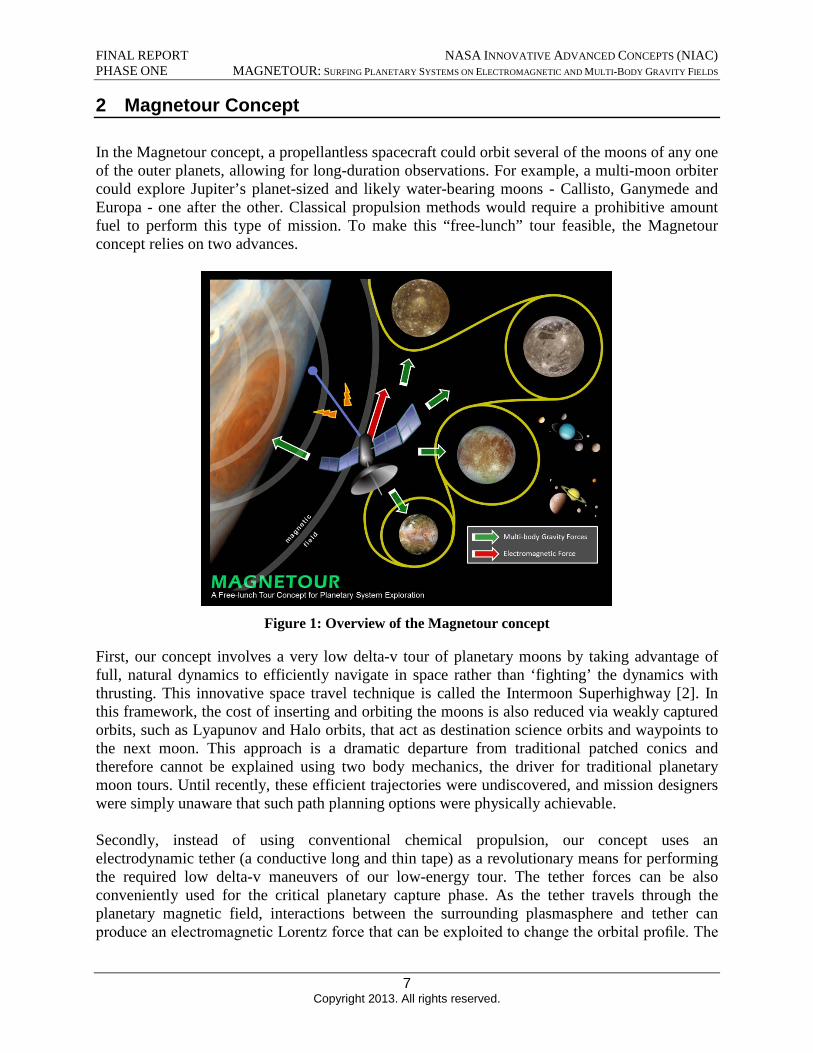
In the Magnetour concept, a propellantless spacecraft could orbit several of the moons of any one of the outer planets, allowing for long-duration observations. For example, a multi-moon orbiter could explore Jupiter’s planet-sized and likely water-bearing moons - Callisto, Ganymede and Europa - one after the other. Classical propulsion methods would require a prohibitive amount fuel to perform this type of mission. To make this “free-lunch” tour feasible, the Magnetour concept relies on two advances.
Figure 1: Overview of the Magnetour concept
First, our concept involves a very low delta-v tour of planetary moons by taking advantage of full, natural dynamics to efficiently navigate in space rather than ‘fighting’ the dynamics with thrusting. This innovative space travel technique is called the Intermoon Superhighway [2]. In this framework, the cost of inserting and orbiting the moons is also reduced via weakly captured orbits, such as Lyapunov and Halo orbits, that act as destination science orbits and waypoints to the next moon. This approach is a dramatic departure from traditional patched conics and therefore cannot be explained using two body mechanics, the driver for traditional planetary moon tours. Until recently, these efficient trajectories were undiscovered, and mission designers were simply unaware that such path planning options were physically achievable.
Secondly, instead of using conventional chemical propulsion, our concept uses an electrodynamic tether (a conductive long and thin tape) as a revolutionary means for performing the required low delta-v maneuvers of our low-energy tour. The tether forces can be also conveniently used for the critical planetary capture phase. As the tether travels through the planetary magnetic field, interactions between the surrounding plasmasphere and tether can produce an electromagnetic Lorentz force that can be exploited to change the orbital profile. The
7 Copyright 2013. All rights reserved.
FINAL REPORT NASA INNOVATIVE ADVANCED CONCEPTS (NIAC) PHASE ONE MAGNETOUR: SURFING PLANETARY SYSTEMS ON ELECTROMAGNETIC AND MULTI-BODY GRAVITY FIELDS
electromagnetic system could also serve as its own power source by plugging in an electric load where convenient; in particular a large energy could be tapped from the big power developed during capture, with negligible effect on the dynamics. By switching on and off the electromagnetic system in specifically designed sequences, the orbit could be made to evolve without recourse to propellant and on-board power sources. A low-energy planetary tour, involving navigation through the moon system and gravitational capture, would therefore offer a perfect opportunity to exploit this idea. While this application is particularly promising in the Jovian system where the magnetic field is rotating fast and is exceptionally strong, the proposed concept could benefit future missions to any of the gas giant moon systems.
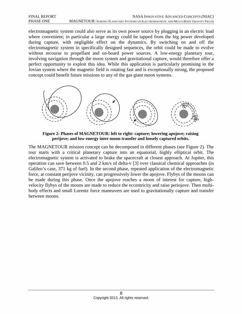
Figure 2: Phases of MAGNETOUR: left to right: capture; lowering apojove; raising perijove; and low-energy inter-moon transfer and loosely captured orbits.
The MAGNETOUR mission concept can be decomposed in different phases (see Figure 2). The tour starts with a critical planetary capture into an equatorial, highly elliptical orbit. The electromagnetic system is activated to brake the spacecraft at closest approach. At Jupiter, this operation can save between 0.5 and 2 km/s of delta-v [3] over classical chemical approaches (in Galileo’s case, 371 kg of fuel). In the second phase, repeated application of the electromagnetic force, at constant perijove vicinity, can progressively lower the apojove. Flybys of the moons can be made during this phase. Once the apojove reaches a moon of interest for capture, high-velocity flybys of the moons are made to reduce the eccentricity and raise periojove. Then multi-body effects and small Lorentz force maneuvers are used to gravitationally capture and transfer between moons.
8 Copyright 2013. All rights reserved.
FINAL REPORT NASA INNOVATIVE ADVANCED CONCEPTS (NIAC) PHASE ONE MAGNETOUR: SURFING PLANETARY SYSTEMS ON ELECTROMAGNETIC AND MULTI-BODY GRAVITY FIELDS
3 Phase One Methodology & Main Findings
The main goals of our Phase 1 study were to characterize the outer planet environments, assess the performance of electrodynamic tethers, explore the coupled behavior of magnetic and gravitational dynamics, confirm feasibility of the concept by designing a propellantless trajectory baseline capable of orbiting multiple moons at Jupiter, and identify science and engineering applications enabled by Magnetour. In this section, the Phase 1 methodology driven by these objectives and the associated key results are summarized. The full details of the larger project tasks can be found in the next sections.
3.1 Study Approach
Conduct literature review & encourage expert interactions
A lot of research has been previously done on electrodynamic tethers. Therefore, a student at University of Texas canvased the various relevant research publications to improve our background on the physics and applications of electrodynamic tethers. His in-depth literature review summarized more than 40 publications, conference presentation and independent reports.
In addition, another way to gain knowledge on the subjects associated to Magnetour was to take advantage of worldclass expertise of JPL in mission design, with many individuals involved in challenging interplanetary missions. In order to take advantage of this knowledge, in the early stages of the Phase 1 study, we gave two presentations, at the Numerical Algorithms for Space Flight (NASF) seminar of the JPL Mission Design & Navigation section. We received a lot of useful feedbacks that helped us improve our research plans. Other sources of knowledge included oneon-one interactions and interviews with experts in space tethers at JPL, such as Marco Quadrelli. Moreover, besides the NIAC symposia, part of our Phase 1 research will be presented at the 2013 Astrodynamics Specialist Conference (Hilton Head, South Carolina, August 2013) [4], which will be an excellent opportunity to disseminate our ideas and interact with industry, government and academia experts.
Formulate simplified models of technical principles
Simplified models for the electrodynamic and multi-body gravitational forces were formulated. These models can be used to provide theoretical estimates of the concept expected performance.
Assess technical & programmatic feasibility by doing a preliminary Jovian mission design
Based on the models of the dynamics, we started assessing the technical and programmatic feasibility of Magnetour on a reference mission. Since the application is particulary promising at Jupiter (see section 4.1), we selected a Jovian multi-moon mission. The following three key questions were answered in that context: 1) Is the proposed approach fundamentally feasible ? ; 2) Are there key quantitative advantages compared to conventional approaches ? ; and 3) What are the scenarios of the representative Jovian mission ?
9 Copyright 2013. All rights reserved.
FINAL REPORT NASA INNOVATIVE ADVANCED CONCEPTS (NIAC) PHASE ONE MAGNETOUR: SURFING PLANETARY SYSTEMS ON ELECTROMAGNETIC AND MULTI-BODY GRAVITY FIELDS
Suggest key technology areas & future work activities
We suggest key technology areas that are required to make the Magnetour concept a reality in the future. Future work activities were proposed to further advance the concept.
3.2 Phase One Key Points
First, the environments of the outer planets were described. The four outer planets in the solar system have been observed to have strong magnetic fields, substantial plasma environments, and trapped radiation belts. These characteristics make them suitable for Magnetour, in particular Jupiter which exhibits the strongest fields. While the magnetic field and plasmas around a planet play a key role in generating forces on a tether, the radiation belts around a planet can greatly limit the lifetime of electronic systems of the spacecraft and damage its structural materials. In turn the magnetic field, plasma, and radiations belts interact with each other in a complex fashion. Thus a Phase 1 recommendation is that each of these features needs to be carefully considered and computed in our concept. The Phase 2 study will therefore consider higher-fidelity models for the outer planet environments, in particular at Jupiter.
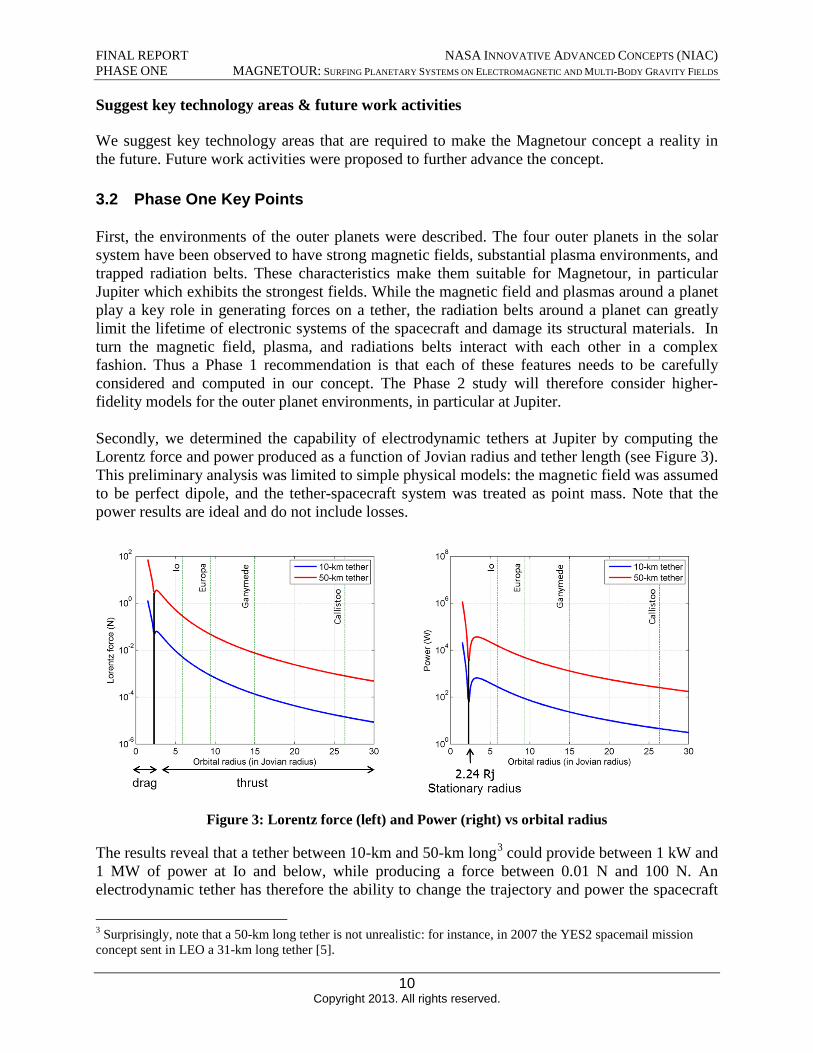
Secondly, we determined the capability of electrodynamic tethers at Jupiter by computing the Lorentz force and power produced as a function of Jovian radius and tether length (see Figure 3). This preliminary analysis was limited to simple physical models: the magnetic field was assumed to be perfect dipole, and the tether-spacecraft system was treated as point mass. Note that the power results are ideal and do not include losses.
Figure 3: Lorentz force (left) and Power (right) vs orbital radius
The results reveal that a tether between 10-km and 50-km long3 could provide between 1 kW and 1 MW of power at Io and below, while producing a force between 0.01 N and 100 N. An electrodynamic tether has therefore the ability to change the trajectory and power the spacecraft
3 Surprisingly, note that a 50-km long tether is not unrealistic: for instance, in 2007 the YES2 spacemail mission concept sent in LEO a 31-km long tether [5].
10 Copyright 2013. All rights reserved.
FINAL REPORT NASA INNOVATIVE ADVANCED CONCEPTS (NIAC) PHASE ONE MAGNETOUR: SURFING PLANETARY SYSTEMS ON ELECTROMAGNETIC AND MULTI-BODY GRAVITY FIELDS
at Io and the other Jovian moonlets. However, farther from Jupiter, in the Ganymede and Callisto regions, the magnetic field is much weaker and therefore the resulting thrust and power suffer a significant drop. Without additional propulsion and power options, in these farther regions, the spacecraft therefore needs to be operated under low power conditions and can perform only small maneuvers. To improve performance of Magnetour, our recommendation for Phase 2 is to investigate the feasibility of combining both electromagnetic and electrostatic tether propulsion techniques using the same bare wire tether hardware, so that significant thrust can be produced in regions of small ambient magnetic field but large ion flux, and vice versa (see section 5.1.2 for more details).
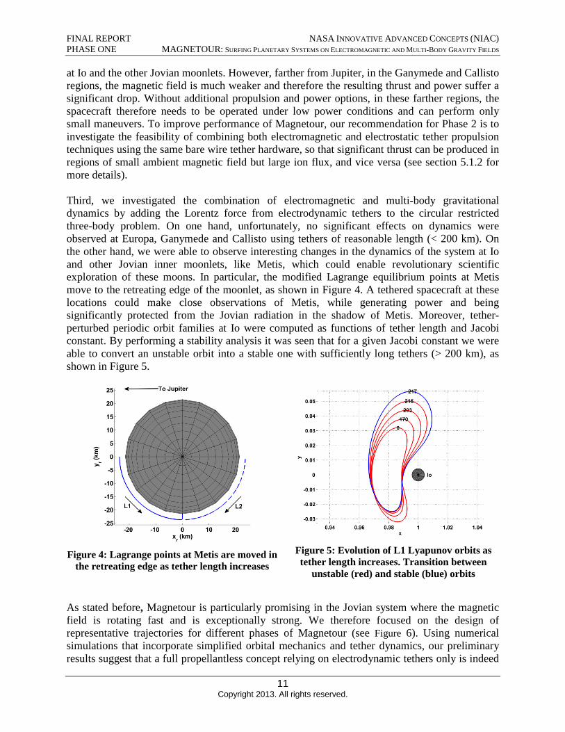
Third, we investigated the combination of electromagnetic and multi-body gravitational dynamics by adding the Lorentz force from electrodynamic tethers to the circular restricted three-body problem. On one hand, unfortunately, no significant effects on dynamics were observed at Europa, Ganymede and Callisto using tethers of reasonable length (< 200 km). On the other hand, we were able to observe interesting changes in the dynamics of the system at Io and other Jovian inner moonlets, like Metis, which could enable revolutionary scientific exploration of these moons. In particular, the modified Lagrange equilibrium points at Metis move to the retreating edge of the moonlet, as shown in Figure 4. A tethered spacecraft at these locations could make close observations of Metis, while generating power and being significantly protected from the Jovian radiation in the shadow of Metis. Moreover, tether-perturbed periodic orbit families at Io were computed as functions of tether length and Jacobi constant. By performing a stability analysis it was seen that for a given Jacobi constant we were able to convert an unstable orbit into a stable one with sufficiently long tethers (> 200 km), as shown in Figure 5.
Figure 4: Lagrange points at Metis are moved in the retreating edge as tether length increases
Figure 5: Evolution of L1 Lyapunov orbits as tether length increases. Transition between
unstable (red) and stable (blue) orbits
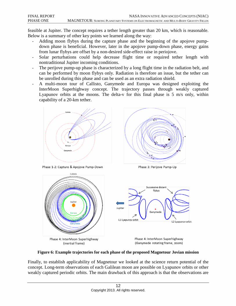
As stated before, Magnetour is particularly promising in the Jovian system where the magnetic field is rotating fast and is exceptionally strong. We therefore focused on the design of representative trajectories for different phases of Magnetour (see Figure 6). Using numerical simulations that incorporate simplified orbital mechanics and tether dynamics, our preliminary results suggest that a full propellantless concept relying on electrodynamic tethers only is indeed
11 Copyright 2013. All rights reserved.
FINAL REPORT NASA INNOVATIVE ADVANCED CONCEPTS (NIAC) PHASE ONE MAGNETOUR: SURFING PLANETARY SYSTEMS ON ELECTROMAGNETIC AND MULTI-BODY GRAVITY FIELDS
feasible at Jupiter. The concept requires a tether length greater than 20 km, which is reasonable. Below is a summary of other key points we learned along the way:
- Adding moon flybys during the capture phase and the beginning of the apojove pump-down phase is beneficial. However, later in the apojove pump-down phase, energy gains from lunar flybys are offset by a non-desired side-effect raise in periojove.
- Solar perturbations could help decrease flight time or required tether length with nontraditional Jupiter incoming conditions.
- The perijove pump-up phase is characterized by a long flight time in the radiation belt, and can be performed by moon flybys only. Radiation is therefore an issue, but the tether can be unrolled during this phase and can be used as an extra radiation shield.
- A multi-moon tour of Callisto, Ganymede and Europa was designed exploiting the InterMoon Superhighway concept. The trajectory passes through weakly captured Lyapunov orbits at the moons. The delta-v for this final phase is 5 m/s only, within capability of a 20-km tether.
Figure 6: Example trajectories for each phase of the proposed Magnetour Jovian mission
Finally, to establish applicability of Magnetour we looked at the science return potential of the concept. Long-term observations of each Galilean moon are possible on Lyapunov orbits or other weakly captured periodic orbits. The main drawback of this approach is that the observations are
12 Copyright 2013. All rights reserved.

FINAL REPORT NASA INNOVATIVE ADVANCED CONCEPTS (NIAC) PHASE ONE MAGNETOUR: SURFING PLANETARY SYSTEMS ON ELECTROMAGNETIC AND MULTI-BODY GRAVITY FIELDS
fairly distant (~ 10,000 km). However, we noted that quasi-ballistic heteroclinic connections between Lyapunov orbits are possible with low-altitude close approaches. Other unique science opportunities of Magnetour are convenient, close observations of the Jovian moonlets and the possibility to use the tether itself as an accurate magnetic sensor.
3.3 Assessment against Phase One Work Plan
The Phase I effort successfully performed all the main four tasks listed in the Phase One proposal work plan. A brief account of the accomplishments for each task and the corresponding sections in the report are given below.
Task 1 – Modeling of electromagnetic system and radiation environment This task was achieved through the simplified modeling of electrodynamic tethers (see section 5.1.1). In addition, a literature review of tether propulsion systems was performed and it was found that electrostatic tethers could be an alternative of interest (see section 5.1.2). Finally, the environment of outer planets was described, with a particular focus on the radiation belts (see section 4).
Task 2 – Explore coupled behavior of magnetic and gravitational dynamics This task was completed by modeling the corresponding perturbed three-body problem, deriving the main properties (perturbed Jacobi constant and Lagrange points) and by computing perturbed Lyapunov periodic orbit families (see section 5.3).
Task 3 – Optimize magneto-assisted trajectories This task was completed by building and analyzing a preliminary Jovian mission point design (see section 7) using electrodynamic tethers. Prototype codes for magneto-assisted capture, apojove pump-down, perijove pump-up and intermoon transfers were developed.
Task 4 – Science definitions and notional cost trades This task was completed by suggesting unique science opportunities offered by Magnetour. In addition, we made approximated mass (~ cost) and radiation comparisons between Magnetour and standard Jovian missions (see sections 7.6 and 7.7).
13 Copyright 2013. All rights reserved.
FINAL REPORT NASA INNOVATIVE ADVANCED CONCEPTS (NIAC) PHASE ONE MAGNETOUR: SURFING PLANETARY SYSTEMS ON ELECTROMAGNETIC AND MULTI-BODY GRAVITY FIELDS
4 Outer Planet Environments
4.1 Overview
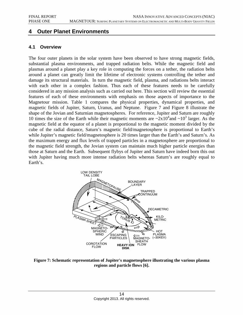
The four outer planets in the solar system have been observed to have strong magnetic fields, substantial plasma environments, and trapped radiation belts. While the magnetic field and plasmas around a planet play a key role in computing the forces on a tether, the radiation belts around a planet can greatly limit the lifetime of electronic systems controlling the tether and damage its structural materials. In turn the magnetic field, plasma, and radiations belts interact with each other in a complex fashion. Thus each of these features needs to be carefully considered in any mission analysis such as carried out here. This section will review the essential features of each of these environments with emphasis on those aspects of importance to the Magnetour mission. Table 1 compares the physical properties, dynamical properties, and magnetic fields of Jupiter, Saturn, Uranus, and Neptune. Figure 7 and Figure 8 illustrate the shape of the Jovian and Saturnian magnetospheres. For reference, Jupiter and Saturn are roughly 10 times the size of the Earth while their magnetic moments are ~2x10⁴and ~103 larger. As the magnetic field at the equator of a planet is proportional to the magnetic moment divided by the cube of the radial distance, Saturn’s magnetic field/magnetosphere is proportional to Earth’s while Jupiter’s magnetic field/magnetosphere is 20 times larger than the Earth’s and Saturn’s. As the maximum energy and flux levels of trapped particles in a magnetosphere are proportional to the magnetic field strength, the Jovian system can maintain much higher particle energies than those at Saturn and the Earth. Subsequent flybys of Jupiter and Saturn have indeed born this out with Jupiter having much more intense radiation belts whereas Saturn’s are roughly equal to Earth’s.
Figure 7: Schematic representation of Jupiter's magnetosphere illustrating the various plasma regions and particle flows [6].
14 Copyright 2013. All rights reserved.
MAGNETO-SPHERIC
WIND ESCAPINGPARTICLES MAGNETO-
SHEATHFLOWCOROTATION
FLOW HEAVY IONDISK
TORUS IO
HOTPLASMA(~30KEV)
KILO-METRIC
DECAMETRIC
MAGNETOPAUSE
BOUNDARYLAYER
PLASMA SHEET
LOW DENSITYTAIL LOBE
TRAPPEDCONTINUUM
FINAL REPORT NASA INNOVATIVE ADVANCED CONCEPTS (NIAC) PHASE ONE MAGNETOUR: SURFING PLANETARY SYSTEMS ON ELECTROMAGNETIC AND MULTI-BODY GRAVITY FIELDS
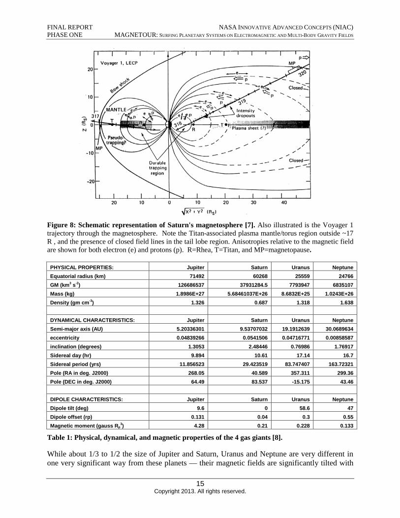
Figure 8: Schematic representation of Saturn's magnetosphere [7]. Also illustrated is the Voyager 1 trajectory through the magnetosphere. Note the Titan-associated plasma mantle/torus region outside ~17 R , and the presence of closed field lines in the tail lobe region. Anisotropies relative to the magnetic field are shown for both electron (e) and protons (p). R=Rhea, T=Titan, and MP=magnetopause.
PHYSICAL PROPERTIES: Jupiter Saturn Uranus Neptune Equatorial radius (km) 71492 60268 25559 24766
-2)GM (km3 s 126686537 37931284.5 7793947 6835107 Mass (kg) 1.8986E+27 5.68461037E+26 8.6832E+25 1.0243E+26 Density (gm cm-3) 1.326 0.687 1.318 1.638
DYNAMICAL CHARACTERISTICS: Jupiter Saturn Uranus Neptune Semi-major axis (AU) 5.20336301 9.53707032 19.1912639 30.0689634 eccentricity 0.04839266 0.0541506 0.04716771 0.00858587 inclination (degrees) 1.3053 2.48446 0.76986 1.76917 Sidereal day (hr) 9.894 10.61 17.14 16.7 Sidereal period (yrs) 11.856523 29.423519 83.747407 163.72321 Pole (RA in deg. J2000) 268.05 40.589 357.311 299.36 Pole (DEC in deg. J2000) 64.49 83.537 -15.175 43.46
DIPOLE CHARACTERISTICS: Jupiter Saturn Uranus Neptune Dipole tilt (deg) 9.6 0 58.6 47 Dipole offset (rp) 0.131 0.04 0.3 0.55 Magnetic moment (gauss Rp
3) 4.28 0.21 0.228 0.133
Table 1: Physical, dynamical, and magnetic properties of the 4 gas giants [8].
While about 1/3 to 1/2 the size of Jupiter and Saturn, Uranus and Neptune are very different in one very significant way from these planets — their magnetic fields are significantly tilted with
15 Copyright 2013. All rights reserved.
FINAL REPORT NASA INNOVATIVE ADVANCED CONCEPTS (NIAC) PHASE ONE MAGNETOUR: SURFING PLANETARY SYSTEMS ON ELECTROMAGNETIC AND MULTI-BODY GRAVITY FIELDS
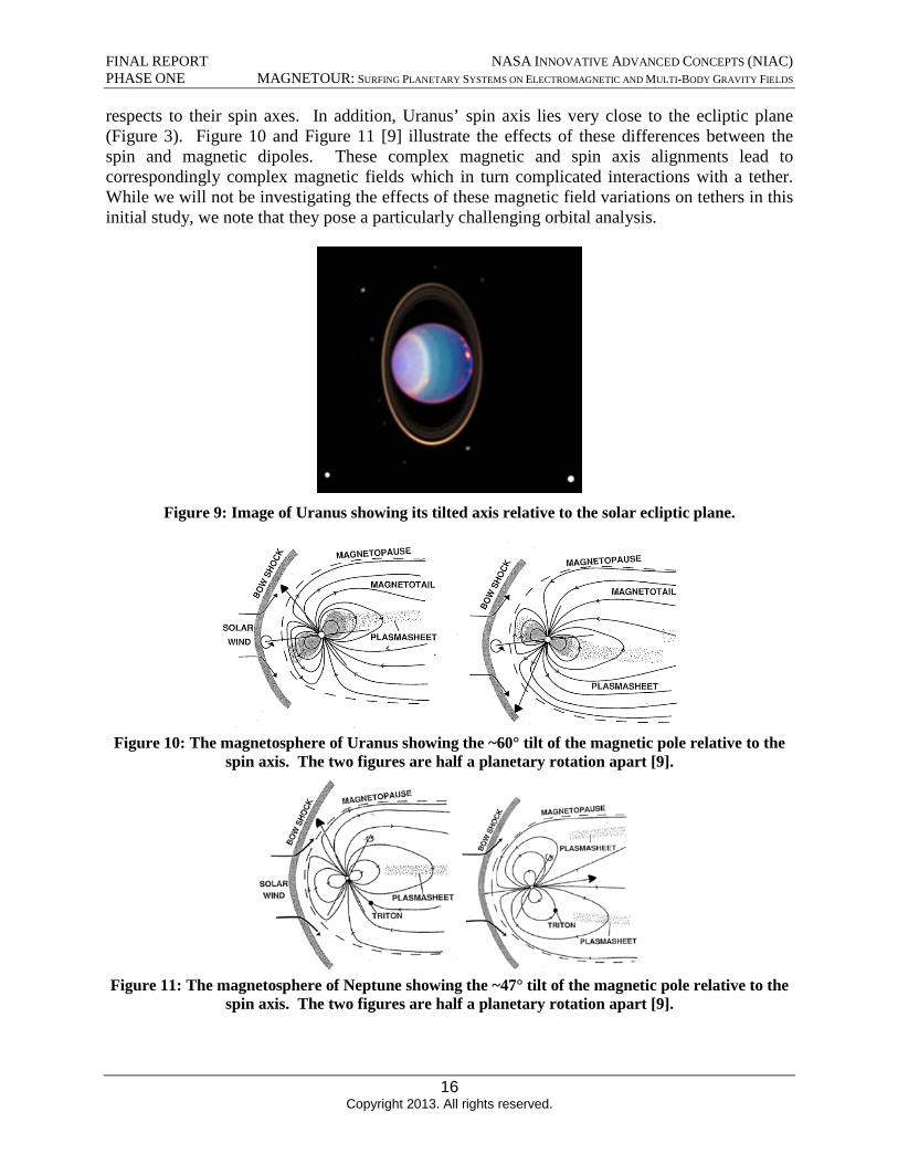
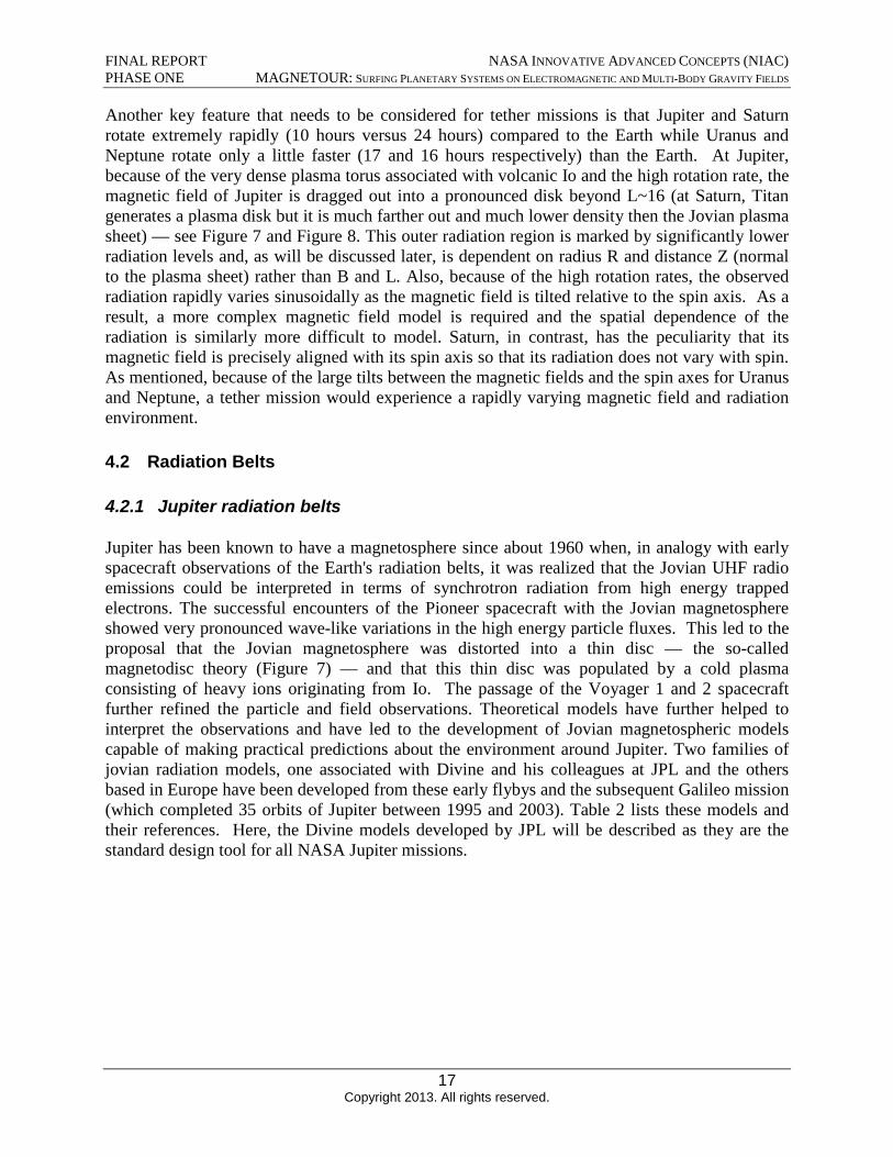
respects to their spin axes. In addition, Uranus’ spin axis lies very close to the ecliptic plane (Figure 3). Figure 10 and Figure 11 [9] illustrate the effects of these differences between the spin and magnetic dipoles. These complex magnetic and spin axis alignments lead to correspondingly complex magnetic fields which in turn complicated interactions with a tether. While we will not be investigating the effects of these magnetic field variations on tethers in this initial study, we note that they pose a particularly challenging orbital analysis.
Figure 9: Image of Uranus showing its tilted axis relative to the solar ecliptic plane.
Figure 10: The magnetosphere of Uranus showing the ~60° tilt of the magnetic pole relative to the spin axis. The two figures are half a planetary rotation apart [9].
Figure 11: The magnetosphere of Neptune showing the ~47° tilt of the magnetic pole relative to the spin axis. The two figures are half a planetary rotation apart [9].
16 Copyright 2013. All rights reserved.
FINAL REPORT NASA INNOVATIVE ADVANCED CONCEPTS (NIAC) PHASE ONE MAGNETOUR: SURFING PLANETARY SYSTEMS ON ELECTROMAGNETIC AND MULTI-BODY GRAVITY FIELDS
Another key feature that needs to be considered for tether missions is that Jupiter and Saturn rotate extremely rapidly (10 hours versus 24 hours) compared to the Earth while Uranus and Neptune rotate only a little faster (17 and 16 hours respectively) than the Earth. At Jupiter, because of the very dense plasma torus associated with volcanic Io and the high rotation rate, the magnetic field of Jupiter is dragged out into a pronounced disk beyond L~16 (at Saturn, Titan generates a plasma disk but it is much farther out and much lower density then the Jovian plasma sheet) — see Figure 7 and Figure 8. This outer radiation region is marked by significantly lower radiation levels and, as will be discussed later, is dependent on radius R and distance Z (normal to the plasma sheet) rather than B and L. Also, because of the high rotation rates, the observed radiation rapidly varies sinusoidally as the magnetic field is tilted relative to the spin axis. As a result, a more complex magnetic field model is required and the spatial dependence of the radiation is similarly more difficult to model. Saturn, in contrast, has the peculiarity that its magnetic field is precisely aligned with its spin axis so that its radiation does not vary with spin. As mentioned, because of the large tilts between the magnetic fields and the spin axes for Uranus and Neptune, a tether mission would experience a rapidly varying magnetic field and radiation environment.
4.2 Radiation Belts
4.2.1 Jupiter radiation belts
Jupiter has been known to have a magnetosphere since about 1960 when, in analogy with early spacecraft observations of the Earth's radiation belts, it was realized that the Jovian UHF radio emissions could be interpreted in terms of synchrotron radiation from high energy trapped electrons. The successful encounters of the Pioneer spacecraft with the Jovian magnetosphere showed very pronounced wave-like variations in the high energy particle fluxes. This led to the proposal that the Jovian magnetosphere was distorted into a thin disc — the so-called magnetodisc theory (Figure 7) — and that this thin disc was populated by a cold plasma consisting of heavy ions originating from Io. The passage of the Voyager 1 and 2 spacecraft further refined the particle and field observations. Theoretical models have further helped to interpret the observations and have led to the development of Jovian magnetospheric models capable of making practical predictions about the environment around Jupiter. Two families of jovian radiation models, one associated with Divine and his colleagues at JPL and the others based in Europe have been developed from these early flybys and the subsequent Galileo mission (which completed 35 orbits of Jupiter between 1995 and 2003). Table 2 lists these models and their references. Here, the Divine models developed by JPL will be described as they are the standard design tool for all NASA Jupiter missions.
17 Copyright 2013. All rights reserved.
FINAL REPORT NASA INNOVATIVE ADVANCED CONCEPTS (NIAC) PHASE ONE MAGNETOUR: SURFING PLANETARY SYSTEMS ON ELECTROMAGNETIC AND MULTI-BODY GRAVITY FIELDS
Table 2: Current Jovian radiation belt models and references
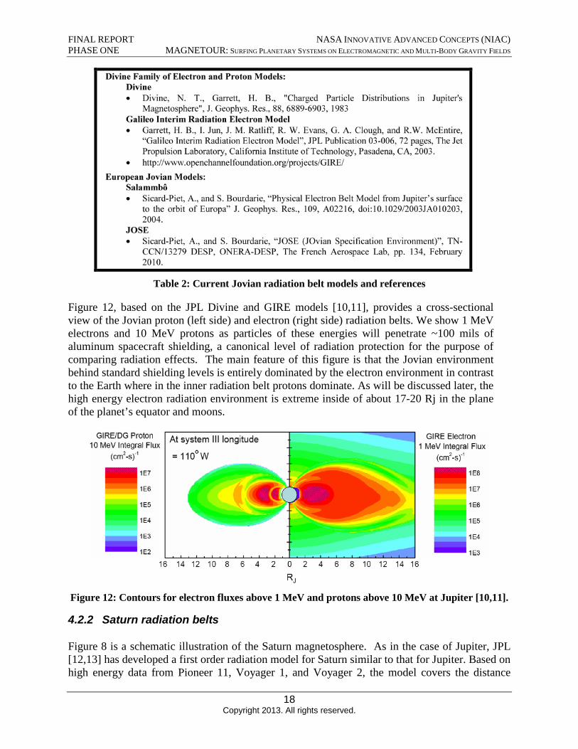
Figure 12, based on the JPL Divine and GIRE models [10,11], provides a cross-sectional view of the Jovian proton (left side) and electron (right side) radiation belts. We show 1 MeV electrons and 10 MeV protons as particles of these energies will penetrate ~100 mils of aluminum spacecraft shielding, a canonical level of radiation protection for the purpose of comparing radiation effects. The main feature of this figure is that the Jovian environment behind standard shielding levels is entirely dominated by the electron environment in contrast to the Earth where in the inner radiation belt protons dominate. As will be discussed later, the high energy electron radiation environment is extreme inside of about 17-20 Rj in the plane of the planet’s equator and moons.
Figure 12: Contours for electron fluxes above 1 MeV and protons above 10 MeV at Jupiter [10,11].
4.2.2 Saturn radiation belts
Figure 8 is a schematic illustration of the Saturn magnetosphere. As in the case of Jupiter, JPL [12,13] has developed a first order radiation model for Saturn similar to that for Jupiter. Based on high energy data from Pioneer 11, Voyager 1, and Voyager 2, the model covers the distance
18 Copyright 2013. All rights reserved.
FINAL REPORT NASA INNOVATIVE ADVANCED CONCEPTS (NIAC) PHASE ONE MAGNETOUR: SURFING PLANETARY SYSTEMS ON ELECTROMAGNETIC AND MULTI-BODY GRAVITY FIELDS
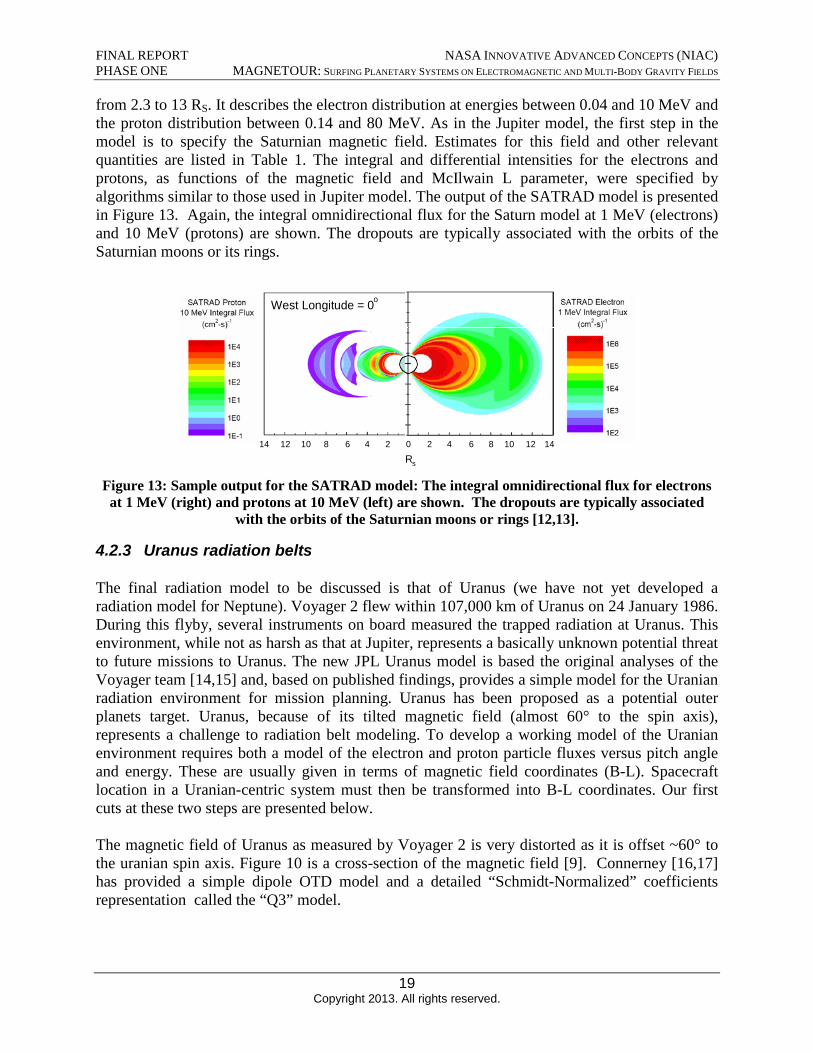
from 2.3 to 13 RS. It describes the electron distribution at energies between 0.04 and 10 MeV and the proton distribution between 0.14 and 80 MeV. As in the Jupiter model, the first step in the model is to specify the Saturnian magnetic field. Estimates for this field and other relevant quantities are listed in Table 1. The integral and differential intensities for the electrons and protons, as functions of the magnetic field and McIlwain L parameter, were specified by algorithms similar to those used in Jupiter model. The output of the SATRAD model is presented in Figure 13. Again, the integral omnidirectional flux for the Saturn model at 1 MeV (electrons) and 10 MeV (protons) are shown. The dropouts are typically associated with the orbits of the Saturnian moons or its rings.
West Longitude = 0o
14 12 10 8 6 4 2 0 2 4 6 8 10 12 14
Rs
Figure 13: Sample output for the SATRAD model: The integral omnidirectional flux for electrons at 1 MeV (right) and protons at 10 MeV (left) are shown. The dropouts are typically associated
with the orbits of the Saturnian moons or rings [12,13].
4.2.3 Uranus radiation belts
The final radiation model to be discussed is that of Uranus (we have not yet developed a radiation model for Neptune). Voyager 2 flew within 107,000 km of Uranus on 24 January 1986. During this flyby, several instruments on board measured the trapped radiation at Uranus. This environment, while not as harsh as that at Jupiter, represents a basically unknown potential threat to future missions to Uranus. The new JPL Uranus model is based the original analyses of the Voyager team [14,15] and, based on published findings, provides a simple model for the Uranian radiation environment for mission planning. Uranus has been proposed as a potential outer planets target. Uranus, because of its tilted magnetic field (almost 60° to the spin axis), represents a challenge to radiation belt modeling. To develop a working model of the Uranian environment requires both a model of the electron and proton particle fluxes versus pitch angle and energy. These are usually given in terms of magnetic field coordinates (B-L). Spacecraft location in a Uranian-centric system must then be transformed into B-L coordinates. Our first cuts at these two steps are presented below.
The magnetic field of Uranus as measured by Voyager 2 is very distorted as it is offset ~60° to the uranian spin axis. Figure 10 is a cross-section of the magnetic field [9]. Connerney [16,17] has provided a simple dipole OTD model and a detailed “Schmidt-Normalized” coefficients representation called the “Q3” model.
19 Copyright 2013. All rights reserved.
FINAL REPORT NASA INNOVATIVE ADVANCED CONCEPTS (NIAC) PHASE ONE MAGNETOUR: SURFING PLANETARY SYSTEMS ON ELECTROMAGNETIC AND MULTI-BODY GRAVITY FIELDS
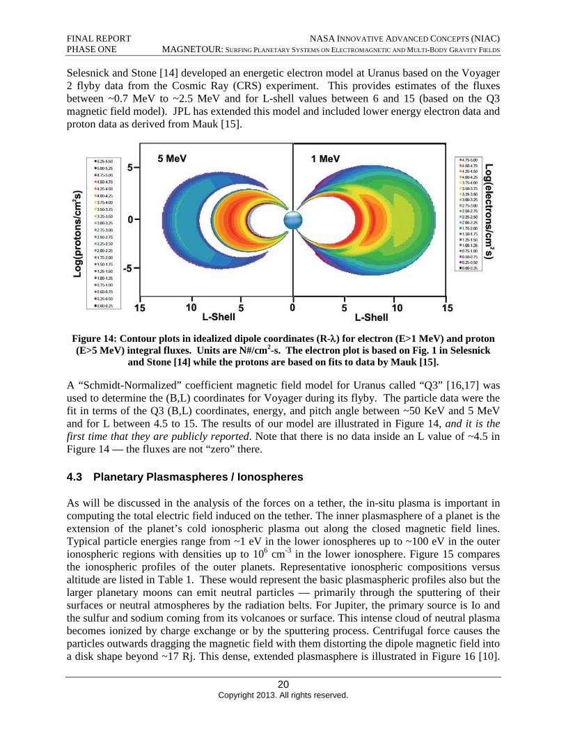
Selesnick and Stone [14] developed an energetic electron model at Uranus based on the Voyager 2 flyby data from the Cosmic Ray (CRS) experiment. This provides estimates of the fluxes between ~0.7 MeV to ~2.5 MeV and for L-shell values between 6 and 15 (based on the Q3 magnetic field model). JPL has extended this model and included lower energy electron data and proton data as derived from Mauk [15].
Figure 14: Contour plots in idealized dipole coordinates (R-λ) for electron (E>1 MeV) and proton (E>5 MeV) integral fluxes. Units are N#/cm2-s. The electron plot is based on Fig. 1 in Selesnick
and Stone [14] while the protons are based on fits to data by Mauk [15].
A “Schmidt-Normalized” coefficient magnetic field model for Uranus called “Q3” [16,17] was used to determine the (B,L) coordinates for Voyager during its flyby. The particle data were the fit in terms of the Q3 (B,L) coordinates, energy, and pitch angle between ~50 KeV and 5 MeV and for L between 4.5 to 15. The results of our model are illustrated in Figure 14, and it is the first time that they are publicly reported. Note that there is no data inside an L value of ~4.5 in Figure 14 — the fluxes are not “zero” there.
4.3 Planetary Plasmaspheres / Ionospheres
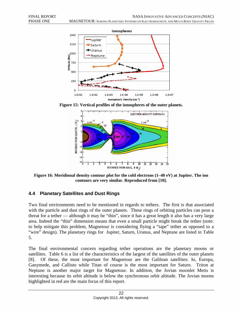
As will be discussed in the analysis of the forces on a tether, the in-situ plasma is important in computing the total electric field induced on the tether. The inner plasmasphere of a planet is the extension of the planet’s cold ionospheric plasma out along the closed magnetic field lines. Typical particle energies range from ~1 eV in the lower ionospheres up to ~100 eV in the outer ionospheric regions with densities up to 106 cm-3 in the lower ionosphere. Figure 15 compares the ionospheric profiles of the outer planets. Representative ionospheric compositions versus altitude are listed in Table 1. These would represent the basic plasmaspheric profiles also but the larger planetary moons can emit neutral particles — primarily through the sputtering of their surfaces or neutral atmospheres by the radiation belts. For Jupiter, the primary source is Io and the sulfur and sodium coming from its volcanoes or surface. This intense cloud of neutral plasma becomes ionized by charge exchange or by the sputtering process. Centrifugal force causes the particles outwards dragging the magnetic field with them distorting the dipole magnetic field into a disk shape beyond ~17 Rj. This dense, extended plasmasphere is illustrated in Figure 16 [10].
20 Copyright 2013. All rights reserved.
Planet
Jupiter Saturn Uranus Neptune
Species + C2H5+ C2H5
+ C2H9 + C2H9
Range(Km) <200
<1000
<400 <250
Species H+
+ H3 H+ H+
+ CH5 H+
Range(Km) >200
1000-6000 >6000
>400 200-300
>300
FINAL REPORT NASA INNOVATIVE ADVANCED CONCEPTS (NIAC) PHASE ONE MAGNETOUR: SURFING PLANETARY SYSTEMS ON ELECTROMAGNETIC AND MULTI-BODY GRAVITY FIELDS
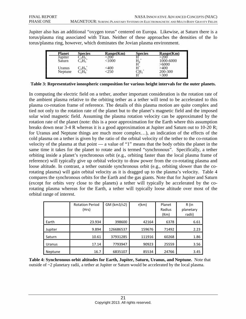
Jupiter also has an additional “oxygen torus” centered on Europa. Likewise, at Saturn there is a torus/plasma ring associated with Titan. Neither of these approaches the densities of the Io torus/plasma ring, however, which dominates the Jovian plasma environment.
Table 3: Representative ionospheric composition for various height intervals for the outer planets.
In computing the electric field on a tether, another important consideration is the rotation rate of the ambient plasma relative to the orbiting tether as a tether will tend to be accelerated to this plasma co-rotation frame of reference. The details of this plasma motion are quite complex and tied not only to the rotation rate of the planet but to the planet’s magnetic field and the imposed solar wind magnetic field. Assuming the plasma rotation velocity can be approximated by the rotation rate of the planet (note: this is a poor approximation for the Earth where this assumption breaks down near 3-4 R whereas it is a good approximation at Jupiter and Saturn out to 10-20 R; for Uranus and Neptune things are much more complex…), an indication of the effects of the cold plasma on a tether is given by the ratio of the orbital velocity of the tether to the co-rotation velocity of the plasma at that point — a value of “1” means that the body orbits the planet in the same time it takes for the planet to rotate and is termed “synchronous”. Specifically, a tether orbiting inside a planet’s synchronous orbit (e.g., orbiting faster than the local plasma frame of reference) will typically give up orbital velocity to draw power from the co-rotating plasma and loose altitude. In contrast, a tether outside synchronous orbit (e.g., orbiting slower than the co-rotating plasma) will gain orbital velocity as it is dragged up to the plasma’s velocity. Table 4 compares the synchronous orbits for the Earth and the gas giants. Note that for Jupiter and Saturn (except for orbits very close to the planets) a tether will typically be accelerated by the co-rotating plasma whereas for the Earth, a tether will typically loose altitude over most of the orbital range of interest.
Rotation Period (Hrs)
GM (km3/s2) r(km) Planet Radius (Km)
R (in planetary
radii)
Earth 23.934 398600 42164 6378 6.61
Jupiter 9.894 126686537 159676 71492 2.23
Saturn 10.61 37931285 111916 60268 1.86
Uranus 17.14 7793947 90923 25559 3.56
Neptune 16.7 6835107 85534 24766 3.45
Table 4: Synchronous orbit altitudes for Earth, Jupiter, Saturn, Uranus, and Neptune. Note that outside of ~2 planetary radii, a tether at Jupiter or Saturn would be accelerated by the local plasma.
21 Copyright 2013. All rights reserved.
FINAL REPORT NASA INNOVATIVE ADVANCED CONCEPTS (NIAC) PHASE ONE MAGNETOUR: SURFING PLANETARY SYSTEMS ON ELECTROMAGNETIC AND MULTI-BODY GRAVITY FIELDS
Figure 15: Vertical profiles of the ionospheres of the outer planets.
Figure 16: Meridional density contour plot for the cold electrons (1–40 eV) at Jupiter. The ion contours are very similar. Reproduced from [10].
4.4 Planetary Satellites and Dust Rings
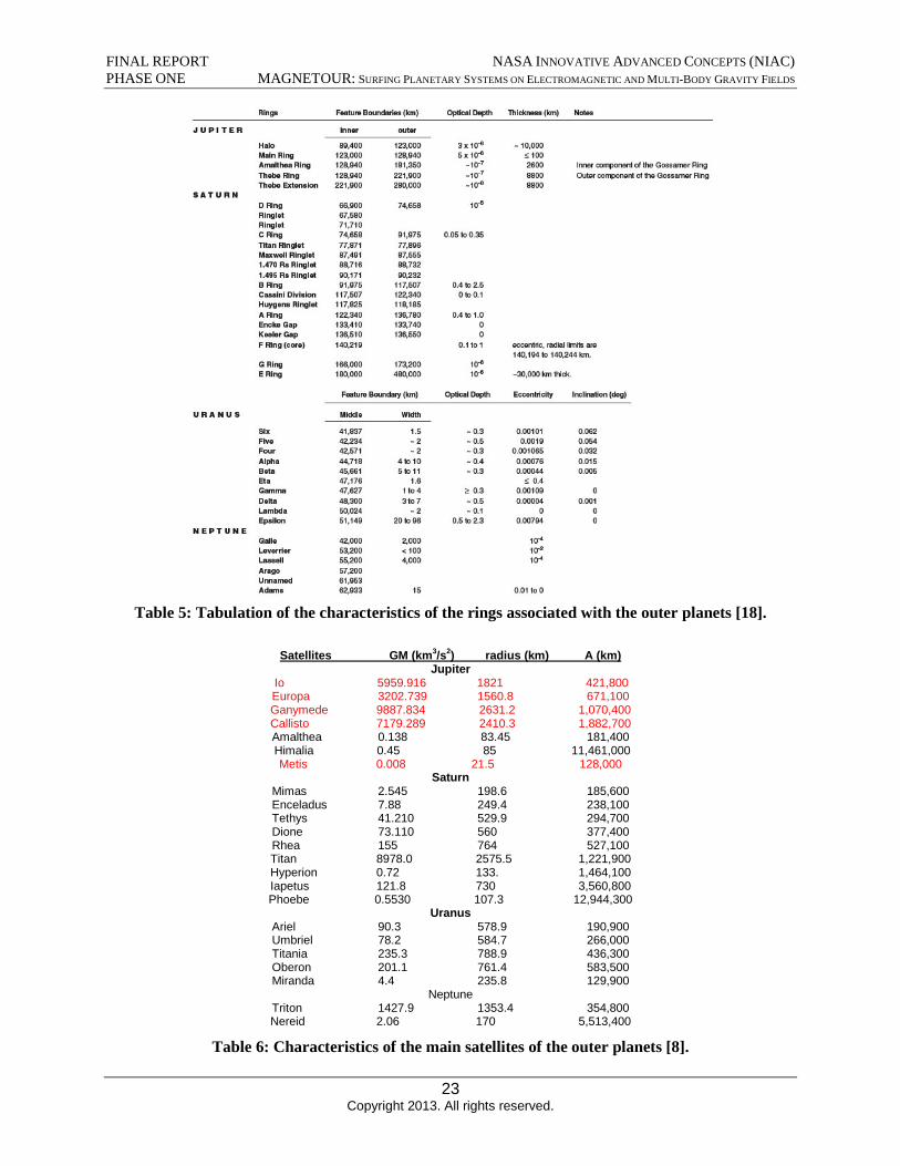
Two final environments need to be mentioned in regards to tethers. The first is that associated with the particle and dust rings of the outer planets. These rings of orbiting particles can pose a threat for a tether — although it may be “thin”, since it has a great length it also has a very large area. Indeed the “thin” dimension means that even a small particle might break the tether (note: to help mitigate this problem, Magnetour is considering flying a “tape” tether as opposed to a “wire” design). The planetary rings for Jupiter, Saturn, Uranus, and Neptune are listed in Table 5.
The final environmental concern regarding tether operations are the planetary moons or satellites. Table 6 is a list of the characteristics of the largest of the satellites of the outer planets [8]. Of these, the most important for Magnetour are the Galilean satellites: Io, Europa, Ganymede, and Callisto while Titan of course is the most important for Saturn. Triton at Neptune is another major target for Magnetour. In addition, the Jovian moonlet Metis is interesting because its orbit altitude is below the synchronous orbit altitude. The Jovian moons highlighted in red are the main focus of this report.
22 Copyright 2013. All rights reserved.
Io 5959.916 1821 421,800
Europa 3202.739 1560.8 671,100 Ganymede 9887.834 2631.2 1,070,400
Callisto 7179.289 2410.3 1,882,700 Amalthea 0.138 83.45 181,400
Himalia 0.45 85 11,461,000 Metis 0.008 21.5 128,000
Mimas 2.545 198.6 185,600
Enceladus 7.88 249.4 238,100 Tethys 41.210 529.9 294,700
Dione 73.110 560 377,400 Rhea 155 764 527,100
Titan 8978.0 2575.5 1,221,900 Hyperion 0.72 133. 1,464,100
Iapetus 121.8 730 3,560,800 Phoebe 0.5530 107.3 12,944,300
Ariel 90.3 578.9 190,900
Umbriel 78.2 584.7 266,000 Titania 235.3 788.9 436,300 Oberon 201.1 761.4 583,500
Miranda 4.4 235.8 129,900
Triton 1427.9 1353.4 354,800 Nereid 2.06 170 5,513,400
FINAL REPORT NASA INNOVATIVE ADVANCED CONCEPTS (NIAC) PHASE ONE MAGNETOUR: SURFING PLANETARY SYSTEMS ON ELECTROMAGNETIC AND MULTI-BODY GRAVITY FIELDS
Table 5: Tabulation of the characteristics of the rings associated with the outer planets [18].
Satellites GM (km3/s2) radius (km) A (km)Jupiter
Saturn
Uranus
Neptune
Table 6: Characteristics of the main satellites of the outer planets [8].
23 Copyright 2013. All rights reserved.
me is the mass of an electron, Em
FINAL REPORT NASA INNOVATIVE ADVANCED CONCEPTS (NIAC) PHASE ONE MAGNETOUR: SURFING PLANETARY SYSTEMS ON ELECTROMAGNETIC AND MULTI-BODY GRAVITY FIELDS
5 Analysis of Basic Technical Principles
5.1 Selecting and Modeling Electromagnetic Systems
We report on our trade studies to select and assess appropriate electromagnetic systems for Magnetour. First we conducted an analysis of the performance of electrodynamic tether systems. Then we suggest investigating further electrostatic tether systems. Finally, we explain why other electromagnetic systems would not be efficient.
5.1.1 Electrodynamic tether
Electrodynamic tethers (EDTs) are bare (uninsulated), conducting wire or tape tethers terminated at one end by a plasma contactor. These tethers could provide both power and propulsion, with just tether hardware accounting for tether subsystem mass. In this subsection, we evaluate the propulsion and power performance of an EDT as a function of tether length.
5.1.1.1 Lorentz force & power
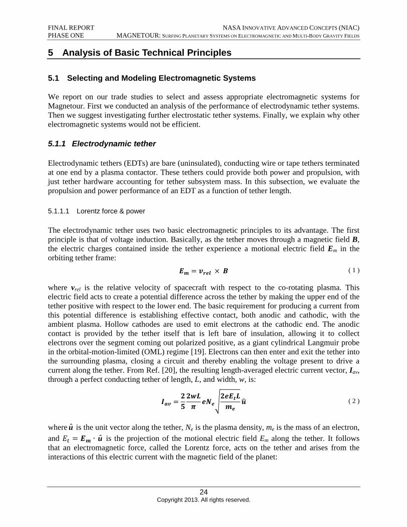
The electrodynamic tether uses two basic electromagnetic principles to its advantage. The first principle is that of voltage induction. Basically, as the tether moves through a magnetic field B, the electric charges contained inside the tether experience a motional electric field Em in the orbiting tether frame:
( 1 ) Em = vrel × B
where vrel is the relative velocity of spacecraft with respect to the co-rotating plasma. This electric field acts to create a potential difference across the tether by making the upper end of the tether positive with respect to the lower end. The basic requirement for producing a current from this potential difference is establishing effective contact, both anodic and cathodic, with the ambient plasma. Hollow cathodes are used to emit electrons at the cathodic end. The anodic contact is provided by the tether itself that is left bare of insulation, allowing it to collect electrons over the segment coming out polarized positive, as a giant cylindrical Langmuir probe in the orbital-motion-limited (OML) regime [19]. Electrons can then enter and exit the tether into the surrounding plasma, closing a circuit and thereby enabling the voltage present to drive a current along the tether. From Ref. [20], the resulting length-averaged electric current vector, Iav, through a perfect conducting tether of length, L, and width, w, is:
2 2wL eNe√
2eEtLIav = u ( 2 ) 5 π me
where u is the unit vector along the tether, Ne is the plasma density, and Et = Em ∙ u is the projection of the motional electric field along the tether. It follows that an electromagnetic force, called the Lorentz force, acts on the tether and arises from the interactions of this electric current with the magnetic field of the planet:
24 Copyright 2013. All rights reserved.
FINAL REPORT PHASE ONE
NASA INNOVATIVE ADVANCED CONCEPTS (NIAC) MAGNETOUR: SURFING PLANETARY SYSTEMS ON ELECTROMAGNETIC AND MULTI-BODY GRAVITY FIELDS
FL = LIav × B
FL = LIav B
( 3 )
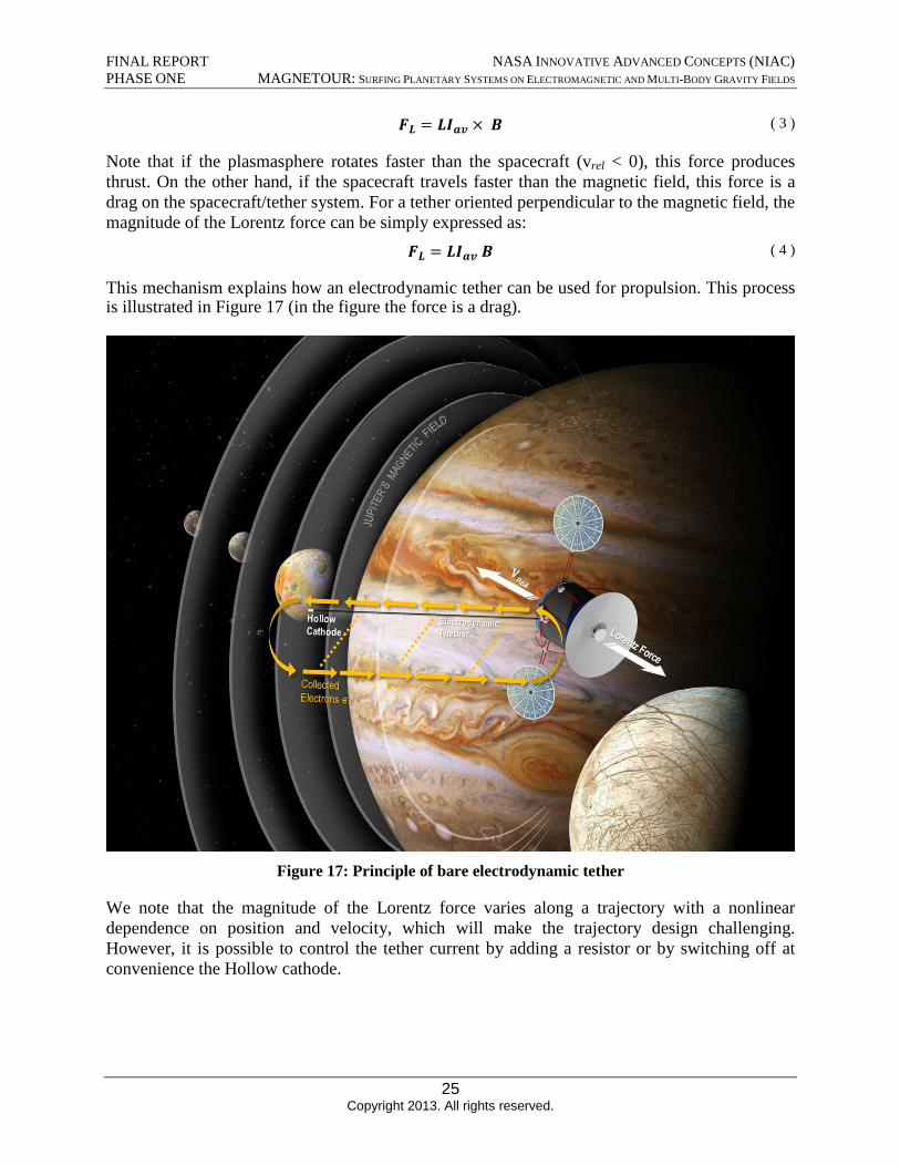
Note that if the plasmasphere rotates faster than the spacecraft (vrel < 0), this force produces thrust. On the other hand, if the spacecraft travels faster than the magnetic field, this force is a drag on the spacecraft/tether system. For a tether oriented perpendicular to the magnetic field, the magnitude of the Lorentz force can be simply expressed as:
( 4 )
This mechanism explains how an electrodynamic tether can be used for propulsion. This processis illustrated in Figure 17 (in the figure the force is a drag).
Figure 17: Principle of bare electrodynamic tether
We note that the magnitude of the Lorentz force varies along a trajectory with a nonlinear dependence on position and velocity, which will make the trajectory design challenging. However, it is possible to control the tether current by adding a resistor or by switching off at convenience the Hollow cathode.
25 Copyright 2013. All rights reserved.
FINAL REPORT NASA INNOVATIVE ADVANCED CONCEPTS (NIAC) PHASE ONE MAGNETOUR: SURFING PLANETARY SYSTEMS ON ELECTROMAGNETIC AND MULTI-BODY GRAVITY FIELDS
In addition to propulsion, the tether can also serve as power source whenever an electric load is plugged in its circuit. The magnitude of the generated power can be expressed in terms of the electromotive force as:
PL = EtLIav ( 5 )
The deployment and Lorentz effects of long electrodynamic tethers were demonstrated by several demo flight missions [21,22]. The SEDS-I and SEDS-II missions successfully deployed 20-km and 7-km non-conductive tethers in 1993 and 1994. Also in 1993, the plasma motorgenerator (PMG) experiment demonstrated the electron collection and current flowing by atethered system. Later, in 1996, the TSS-1R mission, despite ending prematurely by an electricalarc that severed the tether, experienced a 0.4 N electrodynamic drag.
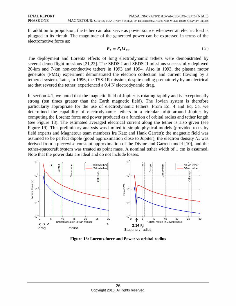
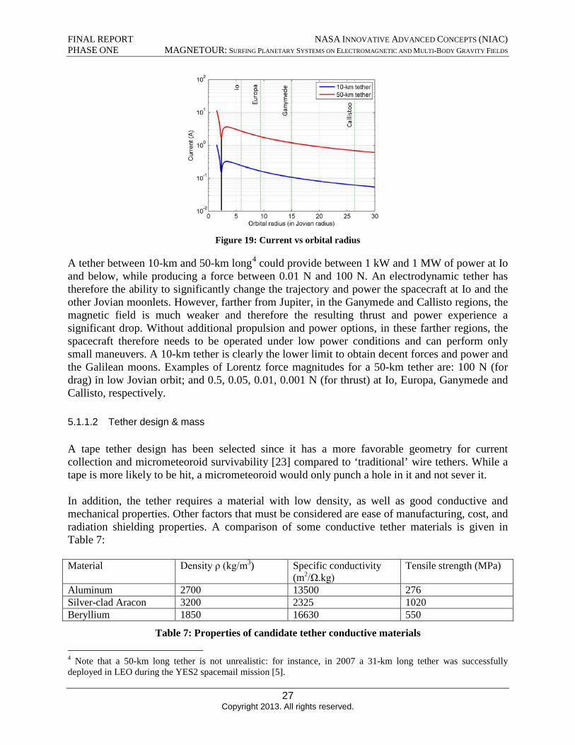
In section 4.1, we noted that the magnetic field of Jupiter is rotating rapidly and is exceptionally strong (ten times greater than the Earth magnetic field). The Jovian system is therefore particularly appropriate for the use of electrodynamic tethers. From Eq. 4 and Eq. 55, we determined the capability of electrodynamic tethers in a circular orbit around Jupiter by computing the Lorentz force and power produced as a function of orbital radius and tether length (see Figure 18). The estimated averaged electrical current along the tether is also given (see Figure 19). This preliminary analysis was limited to simple physical models (provided to us by field experts and Magnetour team members Ira Katz and Hank Garrett): the magnetic field was assumed to be perfect dipole (good approximation close to Jupiter), the electron density Ne was derived from a piecewise constant approximation of the Divine and Garrett model [10], and the tether-spacecraft system was treated as point mass. A nominal tether width of 1 cm is assumed. Note that the power data are ideal and do not include losses.
Figure 18: Lorentz force and Power vs orbital radius
26 Copyright 2013. All rights reserved.
FINAL REPORT NASA INNOVATIVE ADVANCED CONCEPTS (NIAC) PHASE ONE MAGNETOUR: SURFING PLANETARY SYSTEMS ON ELECTROMAGNETIC AND MULTI-BODY GRAVITY FIELDS
Figure 19: Current vs orbital radius
A tether between 10-km and 50-km long4 could provide between 1 kW and 1 MW of power at Io and below, while producing a force between 0.01 N and 100 N. An electrodynamic tether has therefore the ability to significantly change the trajectory and power the spacecraft at Io and the other Jovian moonlets. However, farther from Jupiter, in the Ganymede and Callisto regions, the magnetic field is much weaker and therefore the resulting thrust and power experience a significant drop. Without additional propulsion and power options, in these farther regions, the spacecraft therefore needs to be operated under low power conditions and can perform only small maneuvers. A 10-km tether is clearly the lower limit to obtain decent forces and power and the Galilean moons. Examples of Lorentz force magnitudes for a 50-km tether are: 100 N (for drag) in low Jovian orbit; and 0.5, 0.05, 0.01, 0.001 N (for thrust) at Io, Europa, Ganymede and Callisto, respectively.
5.1.1.2 Tether design & mass
A tape tether design has been selected since it has a more favorable geometry for current collection and micrometeoroid survivability [23] compared to ‘traditional’ wire tethers. While a tape is more likely to be hit, a micrometeoroid would only punch a hole in it and not sever it.
In addition, the tether requires a material with low density, as well as good conductive and mechanical properties. Other factors that must be considered are ease of manufacturing, cost, and radiation shielding properties. A comparison of some conductive tether materials is given in Table 7:
Material Density ρ (kg/m3) Specific conductivity (m2/Ω.kg)
Tensile strength (MPa)
Aluminum 2700 13500 276 Silver-clad Aracon 3200 2325 1020 Beryllium 1850 16630 550
Table 7: Properties of candidate tether conductive materials
4 Note that a 50-km long tether is not unrealistic: for instance, in 2007 a 31-km long tether was successfully deployed in LEO during the YES2 spacemail mission [5].
27 Copyright 2013. All rights reserved.
FINAL REPORT NASA INNOVATIVE ADVANCED CONCEPTS (NIAC) PHASE ONE MAGNETOUR: SURFING PLANETARY SYSTEMS ON ELECTROMAGNETIC AND MULTI-BODY GRAVITY FIELDS
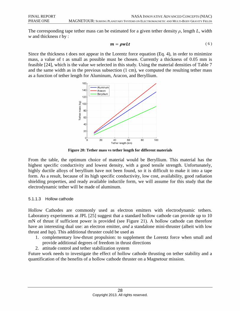
The corresponding tape tether mass can be estimated for a given tether density ρ, length L, width w and thickness t by :
m = ρwLt ( 6 )
Since the thickness t does not appear in the Lorentz force equation (Eq. 4), in order to minimize mass, a value of t as small as possible must be chosen. Currently a thickness of 0.05 mm is feasible [24], which is the value we selected in this study. Using the material densities of Table 7 and the same width as in the previous subsection (1 cm), we computed the resulting tether mass as a function of tether length for Aluminum, Aracon, and Beryllium.
Figure 20: Tether mass vs tether length for different materials
From the table, the optimum choice of material would be Beryllium. This material has the highest specific conductivity and lowest density, with a good tensile strength. Unfortunately, highly ductile alloys of beryllium have not been found, so it is difficult to make it into a tape form. As a result, because of its high specific conductivity, low cost, availability, good radiation shielding properties, and ready available inductile form, we will assume for this study that the electrodynamic tether will be made of aluminum.
5.1.1.3 Hollow cathode
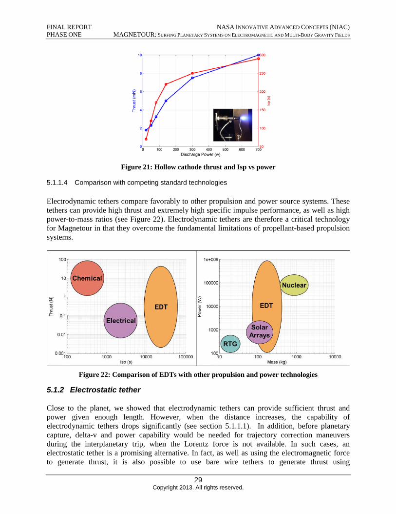
Hollow Cathodes are commonly used as electron emitters with electrodynamic tethers. Laboratory experiments at JPL [25] suggest that a standard hollow cathode can provide up to 10 mN of thrust if sufficient power is provided (see Figure 21). A hollow cathode can therefore have an interesting dual use: an electron emitter, and a standalone mini-thruster (albeit with low thrust and Isp). This additional thruster could be used as
1. complementary low-thrust propulsion: to supplement the Lorentz force when small andprovide additional degrees of freedom in thrust directions
2. attitude control and tether stabilization systemFuture work needs to investigate the effect of hollow cathode thrusting on tether stability and a quantification of the benefits of a hollow cathode thruster on a Magnetour mission.
28 Copyright 2013. All rights reserved.
FINAL REPORT NASA INNOVATIVE ADVANCED CONCEPTS (NIAC) PHASE ONE MAGNETOUR: SURFING PLANETARY SYSTEMS ON ELECTROMAGNETIC AND MULTI-BODY GRAVITY FIELDS
Figure 21: Hollow cathode thrust and Isp vs power
5.1.1.4 Comparison with competing standard technologies
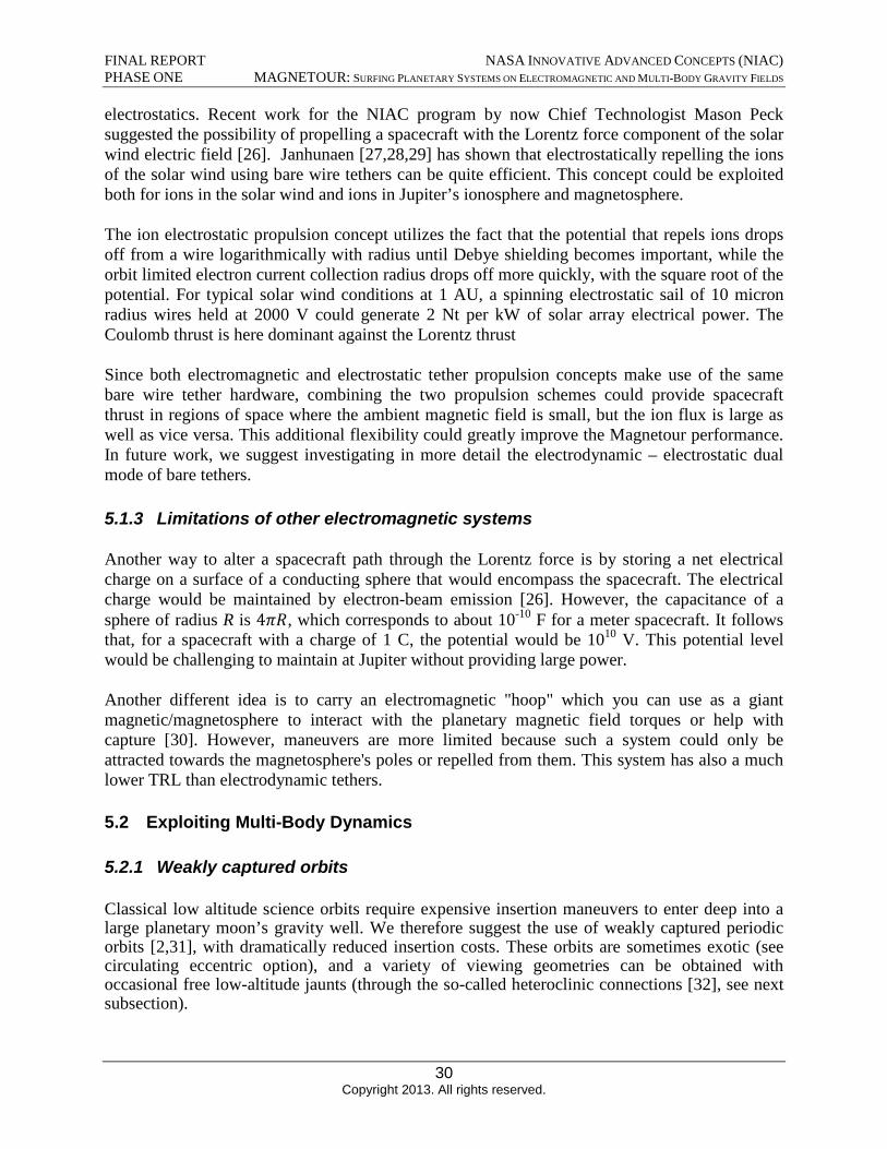
Electrodynamic tethers compare favorably to other propulsion and power source systems. These tethers can provide high thrust and extremely high specific impulse performance, as well as high power-to-mass ratios (see Figure 22). Electrodynamic tethers are therefore a critical technology for Magnetour in that they overcome the fundamental limitations of propellant-based propulsion systems.
Figure 22: Comparison of EDTs with other propulsion and power technologies
5.1.2 Electrostatic tether
Close to the planet, we showed that electrodynamic tethers can provide sufficient thrust and power given enough length. However, when the distance increases, the capability of electrodynamic tethers drops significantly (see section 5.1.1.1). In addition, before planetary capture, delta-v and power capability would be needed for trajectory correction maneuvers during the interplanetary trip, when the Lorentz force is not available. In such cases, an electrostatic tether is a promising alternative. In fact, as well as using the electromagnetic force to generate thrust, it is also possible to use bare wire tethers to generate thrust using
29 Copyright 2013. All rights reserved.
FINAL REPORT NASA INNOVATIVE ADVANCED CONCEPTS (NIAC) PHASE ONE MAGNETOUR: SURFING PLANETARY SYSTEMS ON ELECTROMAGNETIC AND MULTI-BODY GRAVITY FIELDS
electrostatics. Recent work for the NIAC program by now Chief Technologist Mason Peck suggested the possibility of propelling a spacecraft with the Lorentz force component of the solar wind electric field [26]. Janhunaen [27,28,29] has shown that electrostatically repelling the ions of the solar wind using bare wire tethers can be quite efficient. This concept could be exploited both for ions in the solar wind and ions in Jupiter’s ionosphere and magnetosphere.
The ion electrostatic propulsion concept utilizes the fact that the potential that repels ions drops off from a wire logarithmically with radius until Debye shielding becomes important, while the orbit limited electron current collection radius drops off more quickly, with the square root of the potential. For typical solar wind conditions at 1 AU, a spinning electrostatic sail of 10 micron radius wires held at 2000 V could generate 2 Nt per kW of solar array electrical power. The Coulomb thrust is here dominant against the Lorentz thrust
Since both electromagnetic and electrostatic tether propulsion concepts make use of the same bare wire tether hardware, combining the two propulsion schemes could provide spacecraft thrust in regions of space where the ambient magnetic field is small, but the ion flux is large as well as vice versa. This additional flexibility could greatly improve the Magnetour performance. In future work, we suggest investigating in more detail the electrodynamic – electrostatic dual mode of bare tethers.
5.1.3 Limitations of other electromagnetic systems
Another way to alter a spacecraft path through the Lorentz force is by storing a net electrical charge on a surface of a conducting sphere that would encompass the spacecraft. The electrical charge would be maintained by electron-beam emission [26]. However, the capacitance of a sphere of radius R is 4πR, which corresponds to about 10-10 F for a meter spacecraft. It follows that, for a spacecraft with a charge of 1 C, the potential would be 1010 V. This potential level would be challenging to maintain at Jupiter without providing large power.
Another different idea is to carry an electromagnetic "hoop" which you can use as a giant magnetic/magnetosphere to interact with the planetary magnetic field torques or help with capture [30]. However, maneuvers are more limited because such a system could only be attracted towards the magnetosphere's poles or repelled from them. This system has also a much lower TRL than electrodynamic tethers.
5.2 Exploiting Multi-Body Dynamics
5.2.1 Weakly captured orbits
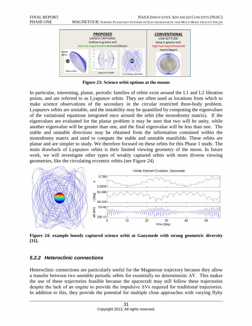
Classical low altitude science orbits require expensive insertion maneuvers to enter deep into alarge planetary moon’s gravity well. We therefore suggest the use of weakly captured periodicorbits [2,31], with dramatically reduced insertion costs. These orbits are sometimes exotic (see circulating eccentric option), and a variety of viewing geometries can be obtained with occasional free low-altitude jaunts (through the so-called heteroclinic connections [32], see nextsubsection).
30 Copyright 2013. All rights reserved.
FINAL REPORT NASA INNOVATIVE ADVANCED CONCEPTS (NIAC) PHASE ONE MAGNETOUR: SURFING PLANETARY SYSTEMS ON ELECTROMAGNETIC AND MULTI-BODY GRAVITY FIELDS
Figure 23: Science orbit options at the moons
In particular, interesting, planar, periodic families of orbits exist around the L1 and L2 libration points, and are referred to as Lyapunov orbits. They are often used as locations from which to make science observations of the secondary in the circular restricted three-body problem. Lyapunov orbits are unstable, and the instability may be quantified by computing the eigenvalues of the variational equations integrated once around the orbit (the monodromy matrix). If the eigenvalues are evaluated for the planar problem it may be seen that two will be unity, while another eigenvalue will be greater than one, and the final eigenvalue will be less than one. The stable and unstable directions may be obtained from the information contained within the monodromy matrix and used to compute the stable and unstable manifolds. These orbits are planar and are simpler to study. We therefore focused on these orbits for this Phase 1 study. The main drawback of Lyapunov orbits is their limited viewing geometry of the moon. In future work, we will investigate other types of weakly captured orbits with more diverse viewing geometries, like the circulating eccentric orbits (see Figure 24)
Figure 24: example loosely captured science orbit at Ganymede with strong geometric diversity [31].
5.2.2 Heteroclinic connections
Heteroclinic connections are particularly useful for the Magnetour trajectory because they allow a transfer between two unstable periodic orbits for essentially no deterministic ΔV. This makes the use of these trajectories feasible because the spacecraft may still follow these trajectories despite the lack of an engine to provide the impulsive ΔVs required for traditional trajectories. In addition to this, they provide the potential for multiple close approaches with varying flyby
31 Copyright 2013. All rights reserved.
FINAL REPORT NASA INNOVATIVE ADVANCED CONCEPTS (NIAC) PHASE ONE MAGNETOUR: SURFING PLANETARY SYSTEMS ON ELECTROMAGNETIC AND MULTI-BODY GRAVITY FIELDS
conditions that would be useful for science observations while providing wide coverage of the surface.
Heteroclinic connections are typically computed by searching for the intersection of the stable and unstable manifolds of these periodic orbits in a surface of section. Simply speaking, the stable manifold Ws of an unstable periodic orbit is composed of those trajectories that approach the orbit as time goes to infinity. The unstable manifold Wu of a periodic orbit is composed of those trajectories that approach that orbit as time goes to negative infinity. Mathematically these intersections are represented as:
u s . ( 7 ) WL1 ∩ WL2
Invariant manifolds have been used to connect libration orbits before [33,34] and heteroclinic connections have also been used with resonant orbits for tour and endgame design [32,35,36,37,38]. Additional specific uses have been found for transfers between orbits in the Sun-Earth and Earth-Moon systems [39,40], and for cases in the elliptic-restricted problem with maneuvers [41,42,43,44,45]. They have also been further used to optimize transfers including maneuvers, and it has been found that they can speed to the design of transfers between trajectories [46].
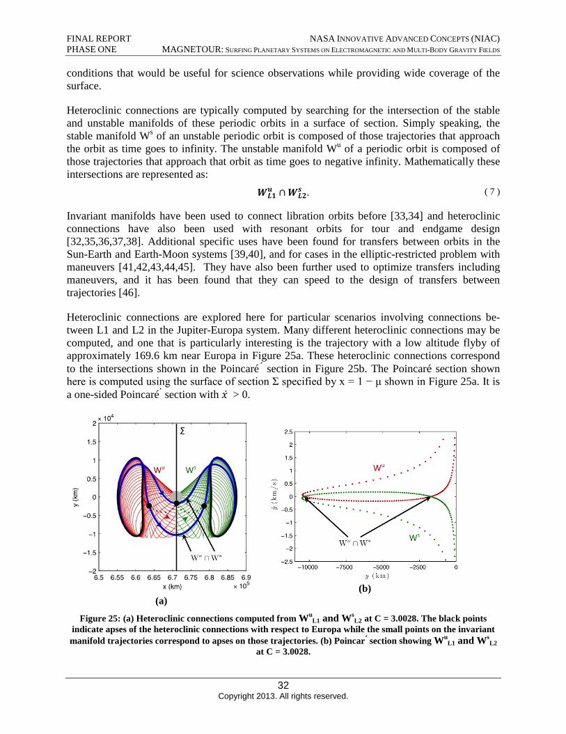
Heteroclinic connections are explored here for particular scenarios involving connections between L1 and L2 in the Jupiter-Europa system. Many different heteroclinic connections may be computed, and one that is particularly interesting is the trajectory with a low altitude flyby of approximately 169.6 km near Europa in Figure 25a. These heteroclinic connections correspond to the intersections shown in the Poincaré section in Figure 25b. The Poincaré section shown here is computed using the surface of section Σ specified by x = 1 − μ shown in Figure 25a. It is a one-sided Poincaré section with x > 0.
(a) (b)
Figure 25: (a) Heteroclinic connections computed from WuL1 and Ws
L2 at C = 3.0028. The black points indicate apses of the heteroclinic connections with respect to Europa while the small points on the invariant manifold trajectories correspond to apses on those trajectories. (b) Poincar section showing Wu
L1 and WsL2
at C = 3.0028.
32 Copyright 2013. All rights reserved.
FINAL REPORT NASA INNOVATIVE ADVANCED CONCEPTS (NIAC) PHASE ONE MAGNETOUR: SURFING PLANETARY SYSTEMS ON ELECTROMAGNETIC AND MULTI-BODY GRAVITY FIELDS
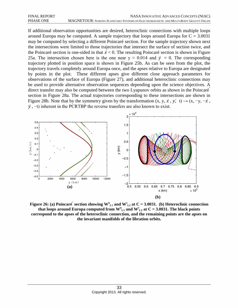
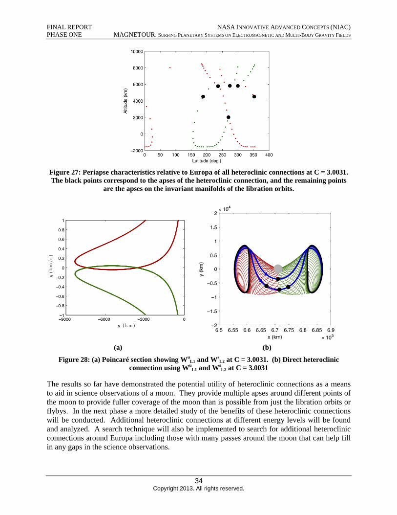
If additional observation opportunities are desired, heteroclinic connections with multiple loops around Europa may be computed. A sample trajectory that loops around Europa for C = 3.0031 may be computed by selecting a different Poincaré section. For the sample trajectory shown next the intersections were limited to those trajectories that intersect the surface of section twice, and the Poincaré section is one-sided in that x < 0. The resulting Poincaré section is shown in Figure 25a. The intersection chosen here is the one near y ≈ 0.014 and y = 0. The corresponding trajectory plotted in position space is shown in Figure 25b. As can be seen from the plot, the trajectory travels completely around Europa once, and the apses relative to Europa are designated by points in the plot. These different apses give different close approach parameters for observations of the surface of Europa (Figure 27), and additional heteroclinic connections may be used to provide alternative observation sequences depending upon the science objectives. A direct transfer may also be computed between the two Lyapunov orbits as shown in the Poincaré section in Figure 28a. The actual trajectories corresponding to these intersections are shown in Figure 28b. Note that by the symmetry given by the transformation (x, y, x , y, t) → (x, −y, −x ,y , −t) inherent in the PCRTBP the reverse transfers are also known to exist.
(a)
(b)
Figure 26: (a) Poincaré section showing WuL1 and Ws
L2 at C = 3.0031. (b) Heteroclinic connection that loops around Europa computed from Wu
L1 and WsL2 at C = 3.0031. The black points
correspond to the apses of the heteroclinic connection, and the remaining points are the apses on the invariant manifolds of the libration orbits.
33 Copyright 2013. All rights reserved.
FINAL REPORT NASA INNOVATIVE ADVANCED CONCEPTS (NIAC) PHASE ONE MAGNETOUR: SURFING PLANETARY SYSTEMS ON ELECTROMAGNETIC AND MULTI-BODY GRAVITY FIELDS
Figure 27: Periapse characteristics relative to Europa of all heteroclinic connections at C = 3.0031. The black points correspond to the apses of the heteroclinic connection, and the remaining points
are the apses on the invariant manifolds of the libration orbits.
(a) (b)
Figure 28: (a) Poincaré section showing WuL1 and Ws
L2 at C = 3.0031. (b) Direct heteroclinic connection using Wu
L1 and WsL2 at C = 3.0031
The results so far have demonstrated the potential utility of heteroclinic connections as a means to aid in science observations of a moon. They provide multiple apses around different points of the moon to provide fuller coverage of the moon than is possible from just the libration orbits or flybys. In the next phase a more detailed study of the benefits of these heteroclinic connections will be conducted. Additional heteroclinic connections at different energy levels will be found and analyzed. A search technique will also be implemented to search for additional heteroclinic connections around Europa including those with many passes around the moon that can help fill in any gaps in the science observations.
34 Copyright 2013. All rights reserved.
FINAL REPORT NASA INNOVATIVE ADVANCED CONCEPTS (NIAC) PHASE ONE MAGNETOUR: SURFING PLANETARY SYSTEMS ON ELECTROMAGNETIC AND MULTI-BODY GRAVITY FIELDS
5.2.3 InterMoon Superhighway
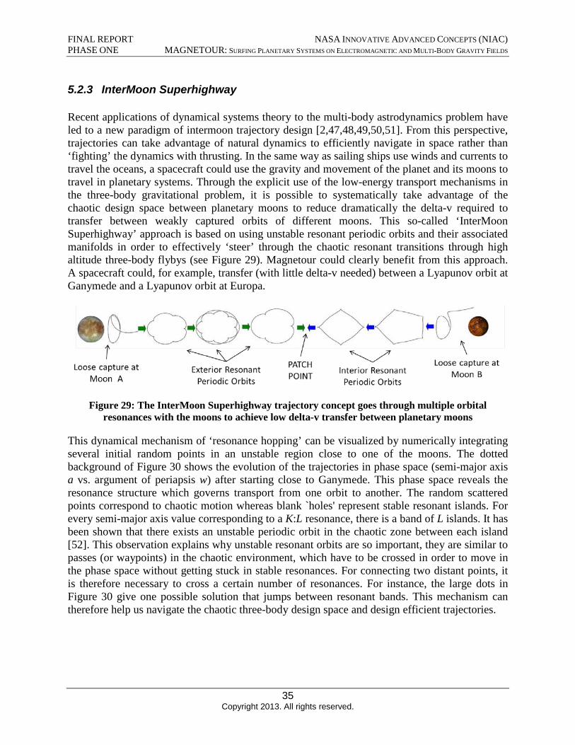
Recent applications of dynamical systems theory to the multi-body astrodynamics problem have led to a new paradigm of intermoon trajectory design [2,47,48,49,50,51]. From this perspective, trajectories can take advantage of natural dynamics to efficiently navigate in space rather than ‘fighting’ the dynamics with thrusting. In the same way as sailing ships use winds and currents to travel the oceans, a spacecraft could use the gravity and movement of the planet and its moons to travel in planetary systems. Through the explicit use of the low-energy transport mechanisms in the three-body gravitational problem, it is possible to systematically take advantage of the chaotic design space between planetary moons to reduce dramatically the delta-v required to transfer between weakly captured orbits of different moons. This so-called ‘InterMoon Superhighway’ approach is based on using unstable resonant periodic orbits and their associated manifolds in order to effectively ‘steer’ through the chaotic resonant transitions through high altitude three-body flybys (see Figure 29). Magnetour could clearly benefit from this approach. A spacecraft could, for example, transfer (with little delta-v needed) between a Lyapunov orbit at Ganymede and a Lyapunov orbit at Europa.
Figure 29: The InterMoon Superhighway trajectory concept goes through multiple orbital resonances with the moons to achieve low delta-v transfer between planetary moons
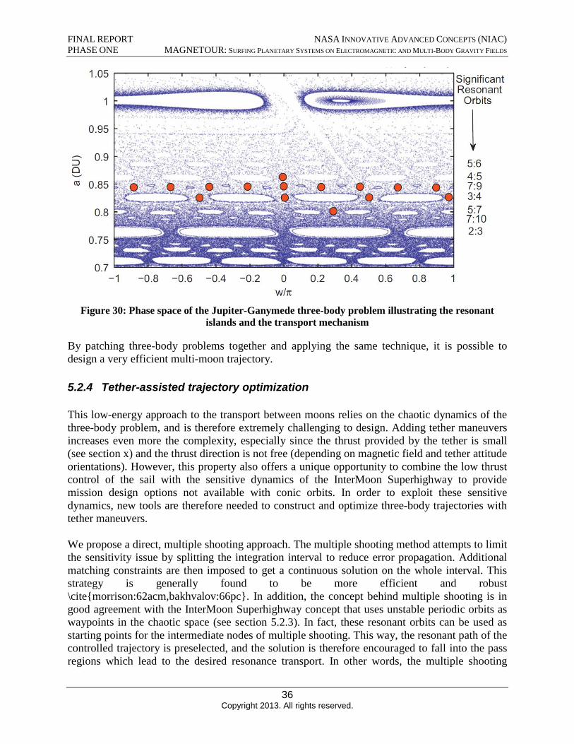
This dynamical mechanism of ‘resonance hopping’ can be visualized by numerically integrating several initial random points in an unstable region close to one of the moons. The dotted background of Figure 30 shows the evolution of the trajectories in phase space (semi-major axis a vs. argument of periapsis w) after starting close to Ganymede. This phase space reveals the resonance structure which governs transport from one orbit to another. The random scattered points correspond to chaotic motion whereas blank `holes' represent stable resonant islands. For every semi-major axis value corresponding to a K:L resonance, there is a band of L islands. It has been shown that there exists an unstable periodic orbit in the chaotic zone between each island [52]. This observation explains why unstable resonant orbits are so important, they are similar to passes (or waypoints) in the chaotic environment, which have to be crossed in order to move in the phase space without getting stuck in stable resonances. For connecting two distant points, it is therefore necessary to cross a certain number of resonances. For instance, the large dots in Figure 30 give one possible solution that jumps between resonant bands. This mechanism can therefore help us navigate the chaotic three-body design space and design efficient trajectories.
35 Copyright 2013. All rights reserved.
FINAL REPORT NASA INNOVATIVE ADVANCED CONCEPTS (NIAC) PHASE ONE MAGNETOUR: SURFING PLANETARY SYSTEMS ON ELECTROMAGNETIC AND MULTI-BODY GRAVITY FIELDS
Figure 30: Phase space of the Jupiter-Ganymede three-body problem illustrating the resonant islands and the transport mechanism
By patching three-body problems together and applying the same technique, it is possible to design a very efficient multi-moon trajectory.
5.2.4 Tether-assisted trajectory optimization
This low-energy approach to the transport between moons relies on the chaotic dynamics of the three-body problem, and is therefore extremely challenging to design. Adding tether maneuvers increases even more the complexity, especially since the thrust provided by the tether is small (see section x) and the thrust direction is not free (depending on magnetic field and tether attitude orientations). However, this property also offers a unique opportunity to combine the low thrust control of the sail with the sensitive dynamics of the InterMoon Superhighway to provide mission design options not available with conic orbits. In order to exploit these sensitive dynamics, new tools are therefore needed to construct and optimize three-body trajectories with tether maneuvers.
We propose a direct, multiple shooting approach. The multiple shooting method attempts to limit the sensitivity issue by splitting the integration interval to reduce error propagation. Additional matching constraints are then imposed to get a continuous solution on the whole interval. This strategy is generally found to be more efficient and robust \cite{morrison:62acm,bakhvalov:66pc}. In addition, the concept behind multiple shooting is in good agreement with the InterMoon Superhighway concept that uses unstable periodic orbits as waypoints in the chaotic space (see section 5.2.3). In fact, these resonant orbits can be used as starting points for the intermediate nodes of multiple shooting. This way, the resonant path of the controlled trajectory is preselected, and the solution is therefore encouraged to fall into the pass regions which lead to the desired resonance transport. In other words, the multiple shooting
36 Copyright 2013. All rights reserved.
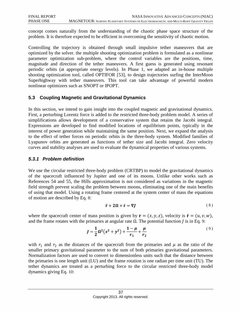
FINAL REPORT NASA INNOVATIVE ADVANCED CONCEPTS (NIAC) PHASE ONE MAGNETOUR: SURFING PLANETARY SYSTEMS ON ELECTROMAGNETIC AND MULTI-BODY GRAVITY FIELDS
concept comes naturally from the understanding of the chaotic phase space structure of the problem. It is therefore expected to be efficient in overcoming the sensitivity of chaotic motion.
Controlling the trajectory is obtained through small impulsive tether maneuvers that are optimized by the solver. the multiple shooting optimization problem is formulated as a nonlinear parameter optimization sub-problem, where the control variables are the positions, time, magnitude and direction of the tether maneuvers. A first guess is generated using resonant periodic orbits (at appropriate energy levels). In Phase 1, we adapted an in-house multiple shooting optimization tool, called OPTIFOR [53], to design trajectories surfing the InterMoon Superhighway with tether maneuvers. This tool can take advantage of powerful modern nonlinear optimizers such as SNOPT or IPOPT.
5.3 Coupling Magnetic and Gravitational Dynamics
In this section, we intend to gain insight into the coupled magnetic and gravitational dynamics. First, a perturbing Lorentz force is added to the restricted three-body problem model. A series of simplifications allows development of a conservative system that retains the Jacobi integral. Expressions are developed to find modified locations of equilibrium points, typically in the interest of power generation while maintaining the same position. Next, we expand the analysis to the effect of tether forces on periodic orbits in the three-body system. Modified families of Lyapunov orbits are generated as functions of tether size and Jacobi integral. Zero velocity curves and stability analyses are used to evaluate the dynamical properties of various systems.
5.3.1 Problem definition
We use the circular restricted three-body problem (CRTBP) to model the gravitational dynamics of the spacecraft influenced by Jupiter and one of its moons. Unlike other works such as References 54 and 55, the Hills approximation is not considered as variations in the magnetic field strength prevent scaling the problem between moons, eliminating one of the main benefits of using that model. Using a rotating frame centered at the system center of mass the equations of motion are described by Eq. 8:
r + 2Ω × r = ∇J ( 8 )
where the spacecraft center of mass position is given by r = (x, y, z), velocity is r = (u, v, w), and the frame rotates with the primaries at angular rate Ω. The potential function J is in Eq. 9:
1 1 − μ μ ( 9 ) J =
2 Ω2(x2 + y2) + +
r1 r2
with r1 and r2 as the distances of the spacecraft from the primaries and μ as the ratio of the smaller primary gravitational parameter to the sum of both primaries gravitational parameters. Normalization factors are used to convert to dimensionless units such that the distance between the primaries is one length unit (LU) and the frame rotation is one radian per time unit (TU). The tether dynamics are treated as a perturbing force to the circular restricted three-body model dynamics giving Eq. 10:
37 Copyright 2013. All rights reserved.
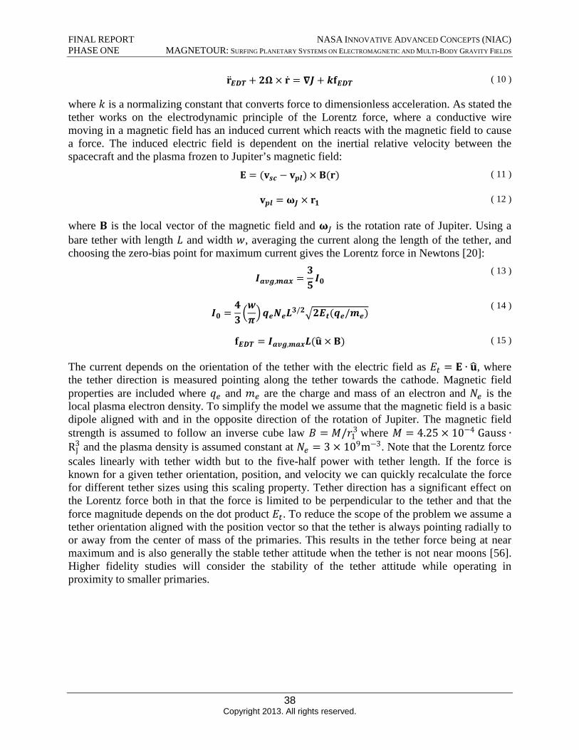
FINAL REPORT NASA INNOVATIVE ADVANCED CONCEPTS (NIAC) PHASE ONE MAGNETOUR: SURFING PLANETARY SYSTEMS ON ELECTROMAGNETIC AND MULTI-BODY GRAVITY FIELDS
r ( 10 ) EDT + 2Ω × r = ∇J + kfEDT
where k is a normalizing constant that converts force to dimensionless acceleration. As stated the tether works on the electrodynamic principle of the Lorentz force, where a conductive wire moving in a magnetic field has an induced current which reacts with the magnetic field to cause a force. The induced electric field is dependent on the inertial relative velocity between the spacecraft and the plasma frozen to Jupiter’s magnetic field:
E = (vsc − vpl) × B(r) ( 11 )
( 12 ) vpl = ωJ × r1
where B is the local vector of the magnetic field and ωJ is the rotation rate of Jupiter. Using a bare tether with length L and width w, averaging the current along the length of the tether, and choosing the zero-bias point for maximum current gives the Lorentz force in Newtons [20]:
3 ( 13 ) =Iavg,max 5
I0
4 ( 14 ) I0 =
3 (wπ)qeNeL3/2√2Et(qe/me)
fEDT = Iavg,maxL(u × B) ( 15 )
The current depends on the orientation of the tether with the electric field as Et = E ∙ u, where the tether direction is measured pointing along the tether towards the cathode. Magnetic field properties are included where qe and me are the charge and mass of an electron and Ne is the local plasma electron density. To simplify the model we assume that the magnetic field is a basic dipole aligned with and in the opposite direction of the rotation of Jupiter. The magnetic field strength is assumed to follow an inverse cube law B = M/r3
1 where M = 4.25 × 10⁻⁴ Gauss ∙R3
J and the plasma density is assumed constant at Ne = 3 × 10⁹m−3. Note that the Lorentz force scales linearly with tether width but to the five-half power with tether length. If the force is known for a given tether orientation, position, and velocity we can quickly recalculate the force for different tether sizes using this scaling property. Tether direction has a significant effect on the Lorentz force both in that the force is limited to be perpendicular to the tether and that the force magnitude depends on the dot product Et . To reduce the scope of the problem we assume a tether orientation aligned with the position vector so that the tether is always pointing radially to or away from the center of mass of the primaries. This results in the tether force being at near maximum and is also generally the stable tether attitude when the tether is not near moons [56]. Higher fidelity studies will consider the stability of the tether attitude while operating in proximity to smaller primaries.
38 Copyright 2013. All rights reserved.
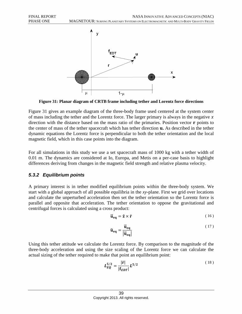
FINAL REPORT NASA INNOVATIVE ADVANCED CONCEPTS (NIAC) PHASE ONE MAGNETOUR: SURFING PLANETARY SYSTEMS ON ELECTROMAGNETIC AND MULTI-BODY GRAVITY FIELDS
Figure 31: Planar diagram of CRTB frame including tether and Lorentz force directions
Figure 31 gives an example diagram of the three-body frame used centered at the system center of mass including the tether and the Lorentz force. The larger primary is always in the negative x direction with the distance based on the mass ratio of the primaries. Position vector r points to the center of mass of the tether spacecraft which has tether direction u. As described in the tether dynamic equations the Lorentz force is perpendicular to both the tether orientation and the local magnetic field, which in this case points into the diagram.
For all simulations in this study we use a set spacecraft mass of 1000 kg with a tether width of 0.01 m. The dynamics are considered at Io, Europa, and Metis on a per-case basis to highlight differences deriving from changes in the magnetic field strength and relative plasma velocity.
5.3.2 Equilibrium points
A primary interest is in tether modified equilibrium points within the three-body system. We start with a global approach of all possible equilibria in the xy-plane. First we grid over locations and calculate the unperturbed acceleration then set the tether orientation so the Lorentz force is parallel and opposite that acceleration. The tether orientation to oppose the gravitational and centrifugal forces is calculated using a cross product:
u-- eq = z × r ( 16 )
u-- ( 17 ) equ =^eq |u-- eq|
Using this tether attitude we calculate the Lorentz force. By comparison to the magnitude of the three-body acceleration and using the size scaling of the Lorentz force we can calculate the actual sizing of the tether required to make that point an equilibrium point:
5⁄2 |r| ( 18 ) =LEQ |fEDT|
L5⁄2
39 Copyright 2013. All rights reserved.
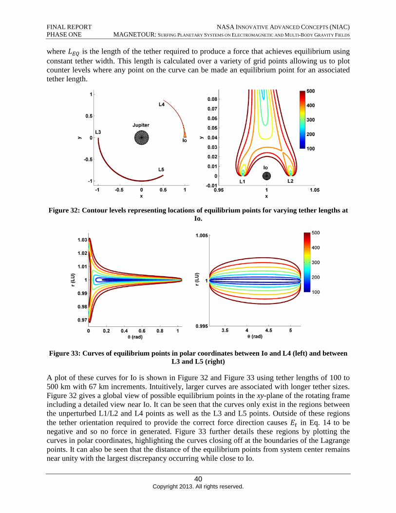
FINAL REPORT NASA INNOVATIVE ADVANCED CONCEPTS (NIAC) PHASE ONE MAGNETOUR: SURFING PLANETARY SYSTEMS ON ELECTROMAGNETIC AND MULTI-BODY GRAVITY FIELDS
where LEQ is the length of the tether required to produce a force that achieves equilibrium using constant tether width. This length is calculated over a variety of grid points allowing us to plot counter levels where any point on the curve can be made an equilibrium point for an associated tether length.
Figure 32: Contour levels representing locations of equilibrium points for varying tether lengths at Io.
Figure 33: Curves of equilibrium points in polar coordinates between Io and L4 (left) and between L3 and L5 (right)
A plot of these curves for Io is shown in Figure 32 and Figure 33 using tether lengths of 100 to 500 km with 67 km increments. Intuitively, larger curves are associated with longer tether sizes. Figure 32 gives a global view of possible equilibrium points in the xy-plane of the rotating frame including a detailed view near Io. It can be seen that the curves only exist in the regions between the unperturbed L1/L2 and L4 points as well as the L3 and L5 points. Outside of these regions the tether orientation required to provide the correct force direction causes Et in Eq. 14 to be negative and so no force in generated. Figure 33 further details these regions by plotting the curves in polar coordinates, highlighting the curves closing off at the boundaries of the Lagrange points. It can also be seen that the distance of the equilibrium points from system center remains near unity with the largest discrepancy occurring while close to Io.
40 Copyright 2013. All rights reserved.
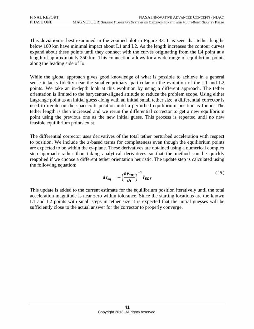
−1
= − (∂rEDT dreq rEDT ∂r
)
FINAL REPORT NASA INNOVATIVE ADVANCED CONCEPTS (NIAC) PHASE ONE MAGNETOUR: SURFING PLANETARY SYSTEMS ON ELECTROMAGNETIC AND MULTI-BODY GRAVITY FIELDS
This deviation is best examined in the zoomed plot in Figure 33. It is seen that tether lengths below 100 km have minimal impact about L1 and L2. As the length increases the contour curves expand about these points until they connect with the curves originating from the L4 point at a length of approximately 350 km. This connection allows for a wide range of equilibrium points along the leading side of Io.
While the global approach gives good knowledge of what is possible to achieve in a general sense it lacks fidelity near the smaller primary, particular on the evolution of the L1 and L2 points. We take an in-depth look at this evolution by using a different approach. The tether orientation is limited to the barycenter-aligned attitude to reduce the problem scope. Using either Lagrange point as an initial guess along with an initial small tether size, a differential corrector is used to iterate on the spacecraft position until a perturbed equilibrium position is found. The tether length is then increased and we rerun the differential corrector to get a new equilibrium point using the previous one as the new initial guess. This process is repeated until no new feasible equilibrium points exist.
The differential corrector uses derivatives of the total tether perturbed acceleration with respect to position. We include the z-based terms for completeness even though the equilibrium points are expected to be within the xy-plane. These derivatives are obtained using a numerical complex step approach rather than taking analytical derivatives so that the method can be quickly reapplied if we choose a different tether orientation heuristic. The update step is calculated using the following equation:
( 19 )
This update is added to the current estimate for the equilibrium position iteratively until the total acceleration magnitude is near zero within tolerance. Since the starting locations are the known L1 and L2 points with small steps in tether size it is expected that the initial guesses will be sufficiently close to the actual answer for the corrector to properly converge.
41 Copyright 2013. All rights reserved.
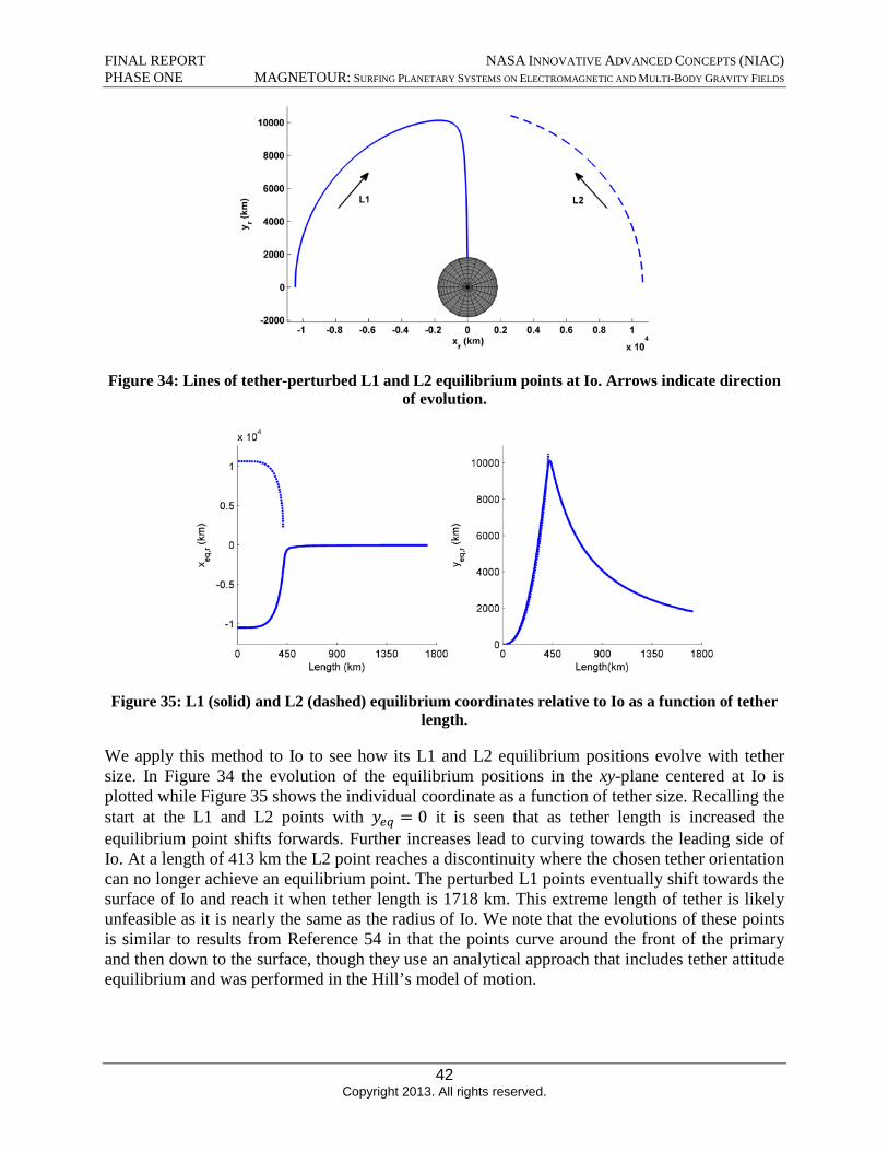
FINAL REPORT NASA INNOVATIVE ADVANCED CONCEPTS (NIAC) PHASE ONE MAGNETOUR: SURFING PLANETARY SYSTEMS ON ELECTROMAGNETIC AND MULTI-BODY GRAVITY FIELDS
Figure 34: Lines of tether-perturbed L1 and L2 equilibrium points at Io. Arrows indicate direction of evolution.
Figure 35: L1 (solid) and L2 (dashed) equilibrium coordinates relative to Io as a function of tether length.
We apply this method to Io to see how its L1 and L2 equilibrium positions evolve with tether size. In Figure 34 the evolution of the equilibrium positions in the xy-plane centered at Io is plotted while Figure 35 shows the individual coordinate as a function of tether size. Recalling the start at the L1 and L2 points with yeq = 0 it is seen that as tether length is increased the equilibrium point shifts forwards. Further increases lead to curving towards the leading side of Io. At a length of 413 km the L2 point reaches a discontinuity where the chosen tether orientation can no longer achieve an equilibrium point. The perturbed L1 points eventually shift towards the surface of Io and reach it when tether length is 1718 km. This extreme length of tether is likely unfeasible as it is nearly the same as the radius of Io. We note that the evolutions of these points is similar to results from Reference 54 in that the points curve around the front of the primary and then down to the surface, though they use an analytical approach that includes tether attitude equilibrium and was performed in the Hill’s model of motion.
42 Copyright 2013. All rights reserved.
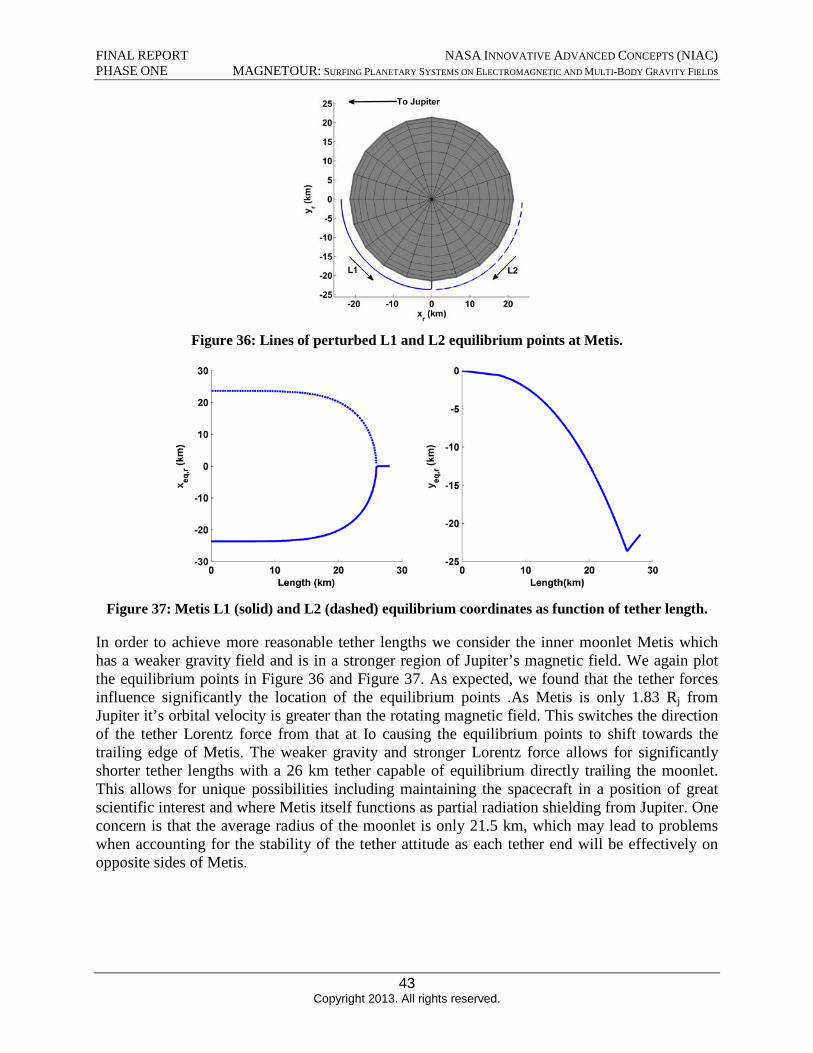
FINAL REPORT NASA INNOVATIVE ADVANCED CONCEPTS (NIAC) PHASE ONE MAGNETOUR: SURFING PLANETARY SYSTEMS ON ELECTROMAGNETIC AND MULTI-BODY GRAVITY FIELDS
Figure 36: Lines of perturbed L1 and L2 equilibrium points at Metis.
Figure 37: Metis L1 (solid) and L2 (dashed) equilibrium coordinates as function of tether length.
In order to achieve more reasonable tether lengths we consider the inner moonlet Metis which has a weaker gravity field and is in a stronger region of Jupiter’s magnetic field. We again plot the equilibrium points in Figure 36 and Figure 37. As expected, we found that the tether forces influence significantly the location of the equilibrium points .As Metis is only 1.83 Rj from Jupiter it’s orbital velocity is greater than the rotating magnetic field. This switches the direction of the tether Lorentz force from that at Io causing the equilibrium points to shift towards the trailing edge of Metis. The weaker gravity and stronger Lorentz force allows for significantly shorter tether lengths with a 26 km tether capable of equilibrium directly trailing the moonlet. This allows for unique possibilities including maintaining the spacecraft in a position of great scientific interest and where Metis itself functions as partial radiation shielding from Jupiter. One concern is that the average radius of the moonlet is only 21.5 km, which may lead to problems when accounting for the stability of the tether attitude as each tether end will be effectively on opposite sides of Metis.
43 Copyright 2013. All rights reserved.
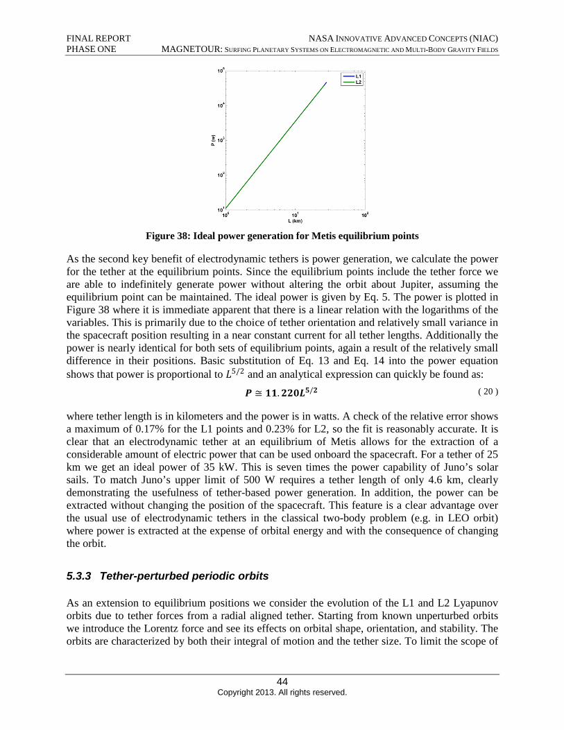
FINAL REPORT NASA INNOVATIVE ADVANCED CONCEPTS (NIAC) PHASE ONE MAGNETOUR: SURFING PLANETARY SYSTEMS ON ELECTROMAGNETIC AND MULTI-BODY GRAVITY FIELDS
Figure 38: Ideal power generation for Metis equilibrium points
As the second key benefit of electrodynamic tethers is power generation, we calculate the power for the tether at the equilibrium points. Since the equilibrium points include the tether force we are able to indefinitely generate power without altering the orbit about Jupiter, assuming the equilibrium point can be maintained. The ideal power is given by Eq. 5. The power is plotted in Figure 38 where it is immediate apparent that there is a linear relation with the logarithms of the variables. This is primarily due to the choice of tether orientation and relatively small variance in the spacecraft position resulting in a near constant current for all tether lengths. Additionally the power is nearly identical for both sets of equilibrium points, again a result of the relatively small difference in their positions. Basic substitution of Eq. 13 and Eq. 14 into the power equation shows that power is proportional to L5/2 and an analytical expression can quickly be found as:
P ≅ 11. 220L5/2 ( 20 )
where tether length is in kilometers and the power is in watts. A check of the relative error shows a maximum of 0.17% for the L1 points and 0.23% for L2, so the fit is reasonably accurate. It is clear that an electrodynamic tether at an equilibrium of Metis allows for the extraction of a considerable amount of electric power that can be used onboard the spacecraft. For a tether of 25 km we get an ideal power of 35 kW. This is seven times the power capability of Juno’s solar sails. To match Juno’s upper limit of 500 W requires a tether length of only 4.6 km, clearly demonstrating the usefulness of tether-based power generation. In addition, the power can be extracted without changing the position of the spacecraft. This feature is a clear advantage over the usual use of electrodynamic tethers in the classical two-body problem (e.g. in LEO orbit) where power is extracted at the expense of orbital energy and with the consequence of changing the orbit.
5.3.3 Tether-perturbed periodic orbits
As an extension to equilibrium positions we consider the evolution of the L1 and L2 Lyapunov orbits due to tether forces from a radial aligned tether. Starting from known unperturbed orbits we introduce the Lorentz force and see its effects on orbital shape, orientation, and stability. The orbits are characterized by both their integral of motion and the tether size. To limit the scope of
44 Copyright 2013. All rights reserved.
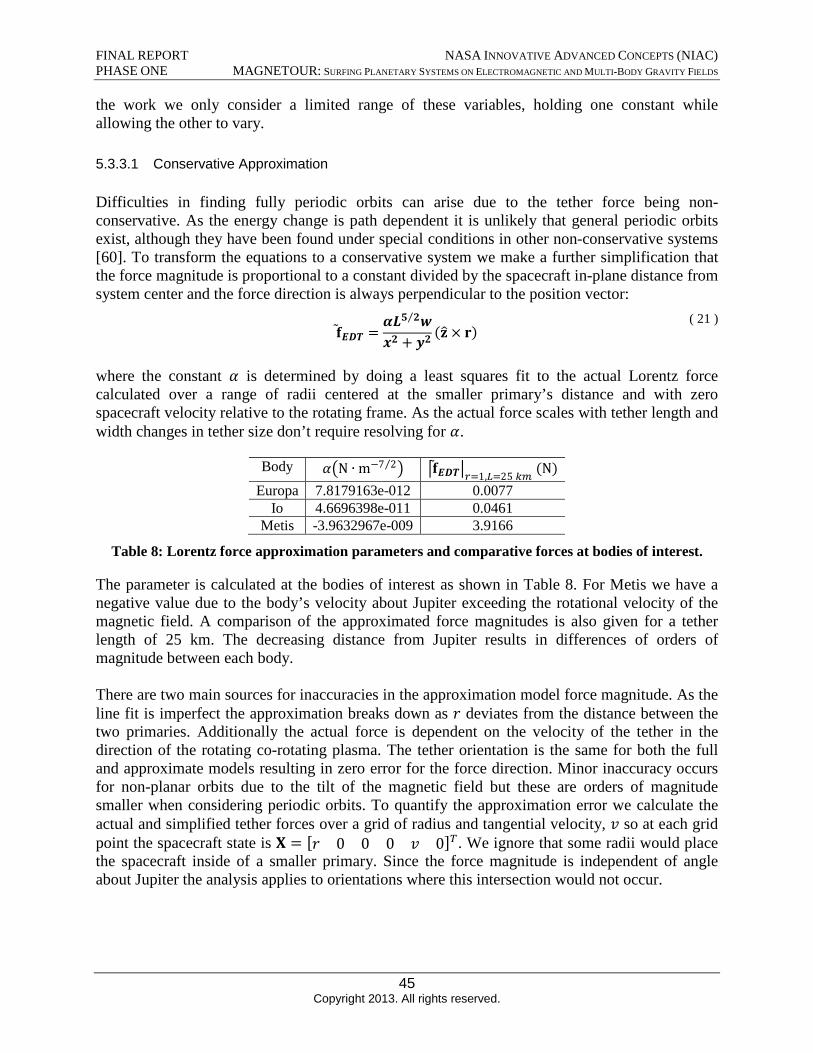
FINAL REPORT NASA INNOVATIVE ADVANCED CONCEPTS (NIAC) PHASE ONE MAGNETOUR: SURFING PLANETARY SYSTEMS ON ELECTROMAGNETIC AND MULTI-BODY GRAVITY FIELDS
the work we only consider a limited range of these variables, holding one constant while allowing the other to vary.
5.3.3.1 Conservative Approximation
Difficulties in finding fully periodic orbits can arise due to the tether force being nonconservative. As the energy change is path dependent it is unlikely that general periodic orbits exist, although they have been found under special conditions in other non-conservative systems [60]. To transform the equations to a conservative system we make a further simplification that the force magnitude is proportional to a constant divided by the spacecraft in-plane distance from system center and the force direction is always perpendicular to the position vector:
αL5⁄2w ( 21 ) =fEDT x2 + y2
(z × r)
where the constant α is determined by doing a least squares fit to the actual Lorentz force calculated over a range of radii centered at the smaller primary’s distance and with zero spacecraft velocity relative to the rotating frame. As the actual force scales with tether length and width changes in tether size don’t require resolving for α.
Body m−7⁄2)α(N ∙ |fEDT|r=1,L=25 km (N)
Europa 7.8179163e-012 0.0077 Io 4.6696398e-011 0.0461
Metis -3.9632967e-009 3.9166
Table 8: Lorentz force approximation parameters and comparative forces at bodies of interest.
The parameter is calculated at the bodies of interest as shown in Table 8. For Metis we have a negative value due to the body’s velocity about Jupiter exceeding the rotational velocity of the magnetic field. A comparison of the approximated force magnitudes is also given for a tether length of 25 km. The decreasing distance from Jupiter results in differences of orders of magnitude between each body.
There are two main sources for inaccuracies in the approximation model force magnitude. As the line fit is imperfect the approximation breaks down as r deviates from the distance between the two primaries. Additionally the actual force is dependent on the velocity of the tether in the direction of the rotating co-rotating plasma. The tether orientation is the same for both the full and approximate models resulting in zero error for the force direction. Minor inaccuracy occurs for non-planar orbits due to the tilt of the magnetic field but these are orders of magnitude smaller when considering periodic orbits. To quantify the approximation error we calculate the actual and simplified tether forces over a grid of radius and tangential velocity, v so at each grid point the spacecraft state is X = [r 0 0 0 v 0]T. We ignore that some radii would place the spacecraft inside of a smaller primary. Since the force magnitude is independent of angle about Jupiter the analysis applies to orientations where this intersection would not occur.
45 Copyright 2013. All rights reserved.
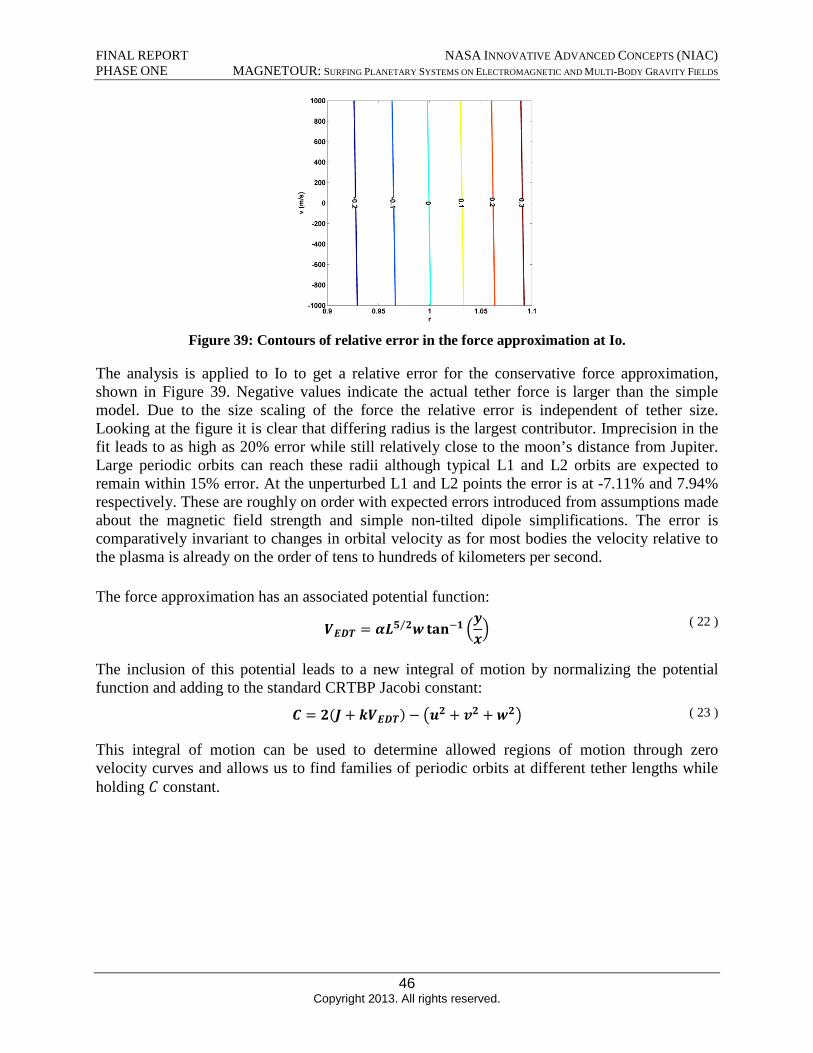
FINAL REPORT NASA INNOVATIVE ADVANCED CONCEPTS (NIAC) PHASE ONE MAGNETOUR: SURFING PLANETARY SYSTEMS ON ELECTROMAGNETIC AND MULTI-BODY GRAVITY FIELDS
Figure 39: Contours of relative error in the force approximation at Io.
The analysis is applied to Io to get a relative error for the conservative force approximation, shown in Figure 39. Negative values indicate the actual tether force is larger than the simple model. Due to the size scaling of the force the relative error is independent of tether size. Looking at the figure it is clear that differing radius is the largest contributor. Imprecision in the fit leads to as high as 20% error while still relatively close to the moon’s distance from Jupiter. Large periodic orbits can reach these radii although typical L1 and L2 orbits are expected to remain within 15% error. At the unperturbed L1 and L2 points the error is at -7.11% and 7.94% respectively. These are roughly on order with expected errors introduced from assumptions made about the magnetic field strength and simple non-tilted dipole simplifications. The error is comparatively invariant to changes in orbital velocity as for most bodies the velocity relative to the plasma is already on the order of tens to hundreds of kilometers per second.
The force approximation has an associated potential function: ( 22 ) VEDT = αL5⁄2w tan−1 (
yx)
The inclusion of this potential leads to a new integral of motion by normalizing the potential function and adding to the standard CRTBP Jacobi constant:
( 23 ) C = 2(J + kVEDT) − (u2 + v2 + w2)
This integral of motion can be used to determine allowed regions of motion through zero velocity curves and allows us to find families of periodic orbits at different tether lengths while holding C constant.
46 Copyright 2013. All rights reserved.
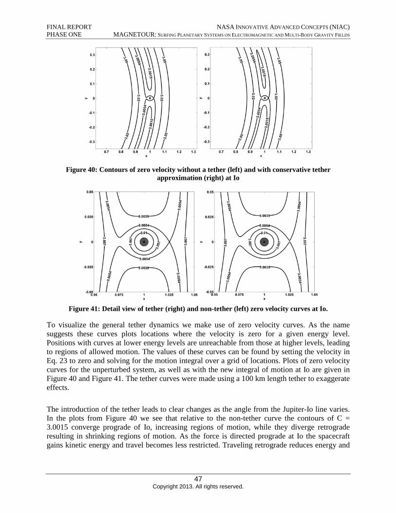
FINAL REPORT NASA INNOVATIVE ADVANCED CONCEPTS (NIAC) PHASE ONE MAGNETOUR: SURFING PLANETARY SYSTEMS ON ELECTROMAGNETIC AND MULTI-BODY GRAVITY FIELDS
Figure 40: Contours of zero velocity without a tether (left) and with conservative tether approximation (right) at Io
Figure 41: Detail view of tether (right) and non-tether (left) zero velocity curves at Io.
To visualize the general tether dynamics we make use of zero velocity curves. As the name suggests these curves plots locations where the velocity is zero for a given energy level. Positions with curves at lower energy levels are unreachable from those at higher levels, leading to regions of allowed motion. The values of these curves can be found by setting the velocity in Eq. 23 to zero and solving for the motion integral over a grid of locations. Plots of zero velocity curves for the unperturbed system, as well as with the new integral of motion at Io are given in Figure 40 and Figure 41. The tether curves were made using a 100 km length tether to exaggerate effects.
The introduction of the tether leads to clear changes as the angle from the Jupiter-Io line varies. In the plots from Figure 40 we see that relative to the non-tether curve the contours of C = 3.0015 converge prograde of Io, increasing regions of motion, while they diverge retrograde resulting in shrinking regions of motion. As the force is directed prograde at Io the spacecraft gains kinetic energy and travel becomes less restricted. Traveling retrograde reduces energy and
47 Copyright 2013. All rights reserved.
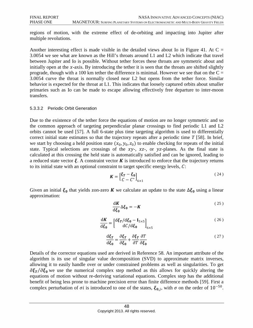
] dK
= [dξT/dξ0 − I5×5
dξ0 dC/dξ0 6×5
dK
∆ξ0 = −Kdξ0
dξT ∂ξT ∂ξT ∂T
= +dξ0 ∂ξ0 ∂T ∂ξ0
∆ξ0
FINAL REPORT NASA INNOVATIVE ADVANCED CONCEPTS (NIAC) PHASE ONE MAGNETOUR: SURFING PLANETARY SYSTEMS ON ELECTROMAGNETIC AND MULTI-BODY GRAVITY FIELDS
regions of motion, with the extreme effect of de-orbiting and impacting into Jupiter after multiple revolutions.
Another interesting effect is made visible in the detailed views about Io in Figure 41. At C = 3.0054 we see what are known as the Hill’s throats around L1 and L2 which indicate that travel between Jupiter and Io is possible. Without tether forces these throats are symmetric about and initially open at the x-axis. By introducing the tether it is seen that the throats are shifted slightly prograde, though with a 100 km tether the difference is minimal. However we see that on the C = 3.0054 curve the throat is normally closed near L2 but opens from the tether force. Similar behavior is expected for the throat at L1. This indicates that loosely captured orbits about smaller primaries such as Io can be made to escape allowing effectively free departure to inter-moon transfers.
5.3.3.2 Periodic Orbit Generation
Due to the existence of the tether force the equations of motion are no longer symmetric and so the common approach of targeting perpendicular planar crossings to find periodic L1 and L2 orbits cannot be used [57]. A full 6-state plus time targeting algorithm is used to differentially correct initial state estimates so that the trajectory repeats after a periodic time T [58]. In brief, we start by choosing a held position state (x0, y0, z0) to enable checking for repeats of the initial state. Typical selections are crossings of the xy-, xz-, or yz-planes. As the final state is calculated at this crossing the held state is automatically satisfied and can be ignored, leading to a reduced state vector ξ. A constraint vector K is introduced to enforce that the trajectory returns to its initial state with an optional constraint to target specific energy levels, C:
K = [ξT − ξ0 ( 24 ) C − C∗ ]
6×1
Given an initial ξ0 that yields zon-zero K we calculate an update to the state using a linear approximation:
( 25 )
( 26 )
( 27 )
Details of the corrector equations used are derived in Reference 58. An important attribute of the algorithm is its use of singular value decomposition (SVD) to approximate matrix inverses, allowing it to easily handle over or under constrained problems as well as singularities. To get∂ξT⁄∂ξ0 we use the numerical complex step method as this allows for quickly altering the equations of motion without re-deriving variational equations. Complex step has the additional benefit of being less prone to machine precision error than finite difference methods [59]. First a complex perturbation of σi is introduced to one of the states, ξ0,j, with σ on the order of 10−50 .
48 Copyright 2013. All rights reserved.
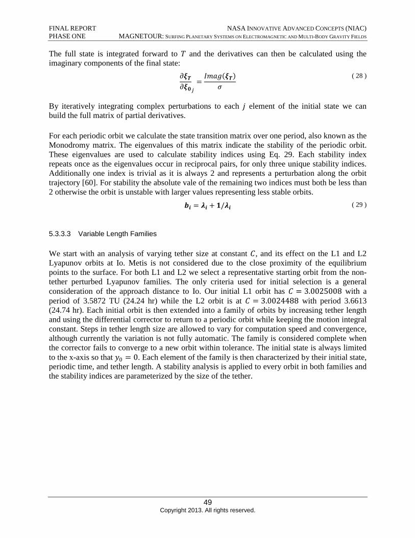
FINAL REPORT NASA INNOVATIVE ADVANCED CONCEPTS (NIAC) PHASE ONE MAGNETOUR: SURFING PLANETARY SYSTEMS ON ELECTROMAGNETIC AND MULTI-BODY GRAVITY FIELDS
The full state is integrated forward to T and the derivatives can then be calculated using the imaginary components of the final state:
∂ξT Imag(ξT) ( 28 ) =
∂ξ0j σ
By iteratively integrating complex perturbations to each j element of the initial state we can build the full matrix of partial derivatives.
For each periodic orbit we calculate the state transition matrix over one period, also known as the Monodromy matrix. The eigenvalues of this matrix indicate the stability of the periodic orbit. These eigenvalues are used to calculate stability indices using Eq. 29. Each stability index repeats once as the eigenvalues occur in reciprocal pairs, for only three unique stability indices. Additionally one index is trivial as it is always 2 and represents a perturbation along the orbit trajectory [60]. For stability the absolute vale of the remaining two indices must both be less than 2 otherwise the orbit is unstable with larger values representing less stable orbits.
bi = λi + 1/λi ( 29 )
5.3.3.3 Variable Length Families
We start with an analysis of varying tether size at constant C, and its effect on the L1 and L2 Lyapunov orbits at Io. Metis is not considered due to the close proximity of the equilibrium points to the surface. For both L1 and L2 we select a representative starting orbit from the non-tether perturbed Lyapunov families. The only criteria used for initial selection is a general consideration of the approach distance to Io. Our initial L1 orbit has C = 3.0025008 with a period of 3.5872 TU (24.24 hr) while the L2 orbit is at C = 3.0024488 with period 3.6613 (24.74 hr). Each initial orbit is then extended into a family of orbits by increasing tether length and using the differential corrector to return to a periodic orbit while keeping the motion integral constant. Steps in tether length size are allowed to vary for computation speed and convergence, although currently the variation is not fully automatic. The family is considered complete when the corrector fails to converge to a new orbit within tolerance. The initial state is always limited to the x-axis so that y0 = 0. Each element of the family is then characterized by their initial state, periodic time, and tether length. A stability analysis is applied to every orbit in both families and the stability indices are parameterized by the size of the tether.
49 Copyright 2013. All rights reserved.
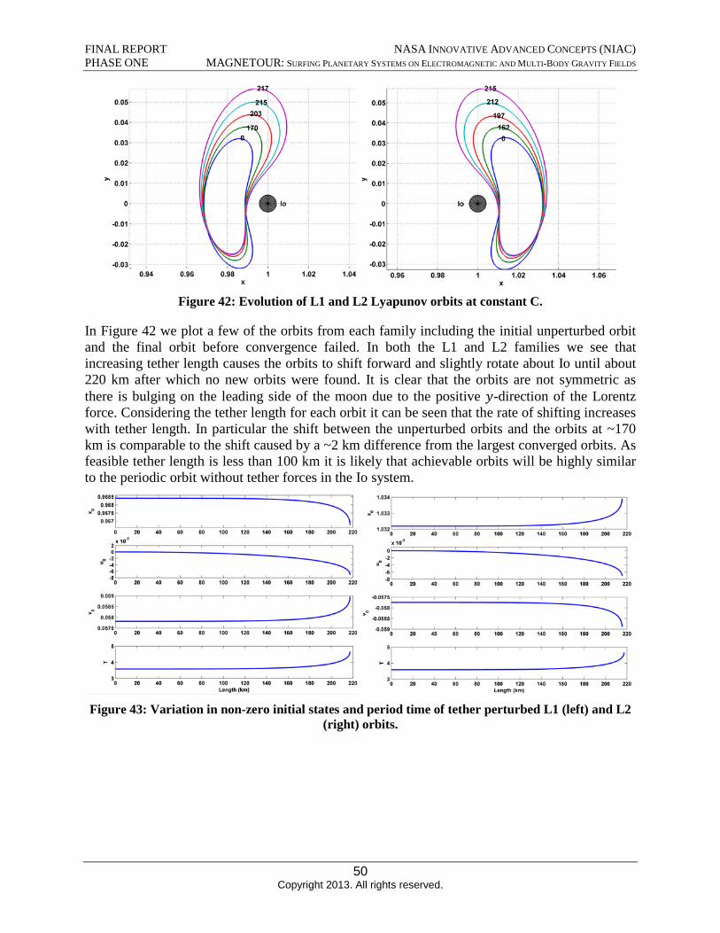
FINAL REPORT NASA INNOVATIVE ADVANCED CONCEPTS (NIAC) PHASE ONE MAGNETOUR: SURFING PLANETARY SYSTEMS ON ELECTROMAGNETIC AND MULTI-BODY GRAVITY FIELDS
Figure 42: Evolution of L1 and L2 Lyapunov orbits at constant C.
In Figure 42 we plot a few of the orbits from each family including the initial unperturbed orbit and the final orbit before convergence failed. In both the L1 and L2 families we see that increasing tether length causes the orbits to shift forward and slightly rotate about Io until about 220 km after which no new orbits were found. It is clear that the orbits are not symmetric as there is bulging on the leading side of the moon due to the positive y-direction of the Lorentz force. Considering the tether length for each orbit it can be seen that the rate of shifting increases with tether length. In particular the shift between the unperturbed orbits and the orbits at ~170 km is comparable to the shift caused by a ~2 km difference from the largest converged orbits. As feasible tether length is less than 100 km it is likely that achievable orbits will be highly similar to the periodic orbit without tether forces in the Io system.
Figure 43: Variation in non-zero initial states and period time of tether perturbed L1 (left) and L2 (right) orbits.
50 Copyright 2013. All rights reserved.
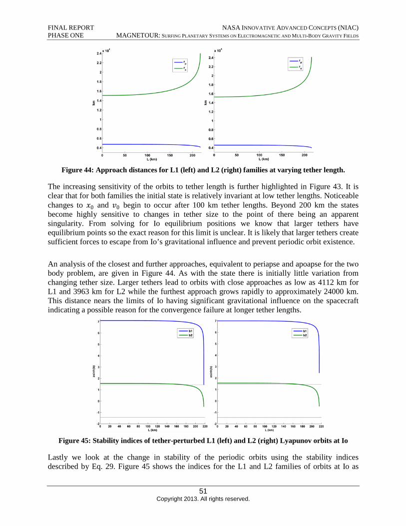
FINAL REPORT NASA INNOVATIVE ADVANCED CONCEPTS (NIAC) PHASE ONE MAGNETOUR: SURFING PLANETARY SYSTEMS ON ELECTROMAGNETIC AND MULTI-BODY GRAVITY FIELDS
Figure 44: Approach distances for L1 (left) and L2 (right) families at varying tether length.
The increasing sensitivity of the orbits to tether length is further highlighted in Figure 43. It is clear that for both families the initial state is relatively invariant at low tether lengths. Noticeable changes to x0 and v0 begin to occur after 100 km tether lengths. Beyond 200 km the states become highly sensitive to changes in tether size to the point of there being an apparent singularity. From solving for Io equilibrium positions we know that larger tethers have equilibrium points so the exact reason for this limit is unclear. It is likely that larger tethers create sufficient forces to escape from Io’s gravitational influence and prevent periodic orbit existence.
An analysis of the closest and further approaches, equivalent to periapse and apoapse for the two body problem, are given in Figure 44. As with the state there is initially little variation from changing tether size. Larger tethers lead to orbits with close approaches as low as 4112 km for L1 and 3963 km for L2 while the furthest approach grows rapidly to approximately 24000 km. This distance nears the limits of Io having significant gravitational influence on the spacecraft indicating a possible reason for the convergence failure at longer tether lengths.
Figure 45: Stability indices of tether-perturbed L1 (left) and L2 (right) Lyapunov orbits at Io
Lastly we look at the change in stability of the periodic orbits using the stability indices described by Eq. 29. Figure 45 shows the indices for the L1 and L2 families of orbits at Io as
51 Copyright 2013. All rights reserved.
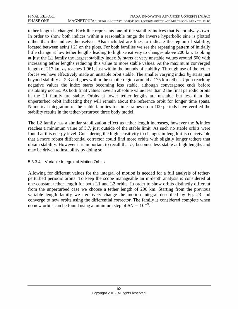
FINAL REPORT NASA INNOVATIVE ADVANCED CONCEPTS (NIAC) PHASE ONE MAGNETOUR: SURFING PLANETARY SYSTEMS ON ELECTROMAGNETIC AND MULTI-BODY GRAVITY FIELDS
tether length is changed. Each line represents one of the stability indices that is not always two. In order to show both indices within a reasonable range the inverse hyperbolic sine is plotted rather than the indices themselves. Also included are lines to indicate the region of stability, located between asin(±2) on the plots. For both families we see the repeating pattern of initially little change at low tether lengths leading to high sensitivity to changes above 200 km. Looking at just the L1 family the largest stability index b1 starts at very unstable values around 600 with increasing tether lengths reducing this value to more stable values. At the maximum converged length of 217 km b1 reaches 1.961, just within the bounds of stability. Through use of the tether forces we have effectively made an unstable orbit stable. The smaller varying index b2 starts just beyond stability at 2.3 and goes within the stabile region around a 175 km tether. Upon reaching negative values the index starts becoming less stable, although convergence ends before instability occurs. As both final values have an absolute value less than 2 the final periodic orbits in the L1 family are stable. Orbits at lower tether lengths are unstable but less than the unperturbed orbit indicating they will remain about the reference orbit for longer time spans. Numerical integration of the stable families for time frames up to 100 periods have verified the stability results in the tether-perturbed three body model.
The L2 family has a similar stabilization effect as tether length increases, however the b1index reaches a minimum value of 5.7, just outside of the stable limit. As such no stable orbits were found at this energy level. Considering the high sensitivity to changes in length it is conceivable that a more robust differential corrector could find more orbits with slightly longer tethers that obtain stability. However it is important to recall that b2 becomes less stable at high lengths and may be driven to instability by doing so.
5.3.3.4 Variable Integral of Motion Orbits
Allowing for different values for the integral of motion is needed for a full analysis of tether-perturbed periodic orbits. To keep the scope manageable an in-depth analysis is considered at one constant tether length for both L1 and L2 orbits. In order to show orbits distinctly different from the unperturbed case we choose a tether length of 200 km. Starting from the previous variable length family we iteratively change the motion integral described by Eq. 23 and converge to new orbits using the differential corrector. The family is considered complete when no new orbits can be found using a minimum step of ∆C = 10−9 .
52 Copyright 2013. All rights reserved.
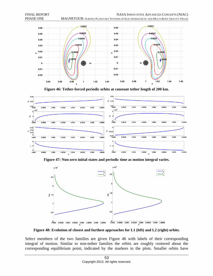
FINAL REPORT NASA INNOVATIVE ADVANCED CONCEPTS (NIAC) PHASE ONE MAGNETOUR: SURFING PLANETARY SYSTEMS ON ELECTROMAGNETIC AND MULTI-BODY GRAVITY FIELDS
Figure 46: Tether-forced periodic orbits at constant tether length of 200 km.
Figure 47: Non-zero initial states and periodic time as motion integral varies.
Figure 48: Evolution of closest and furthest approaches for L1 (left) and L2 (right) orbits.
Select members of the two families are given Figure 46 with labels of their corresponding integral of motion. Similar to non-tether families the orbits are roughly centered about the corresponding equilibrium point, indicated by the markers in the plots. Smaller orbits have
53 Copyright 2013. All rights reserved.
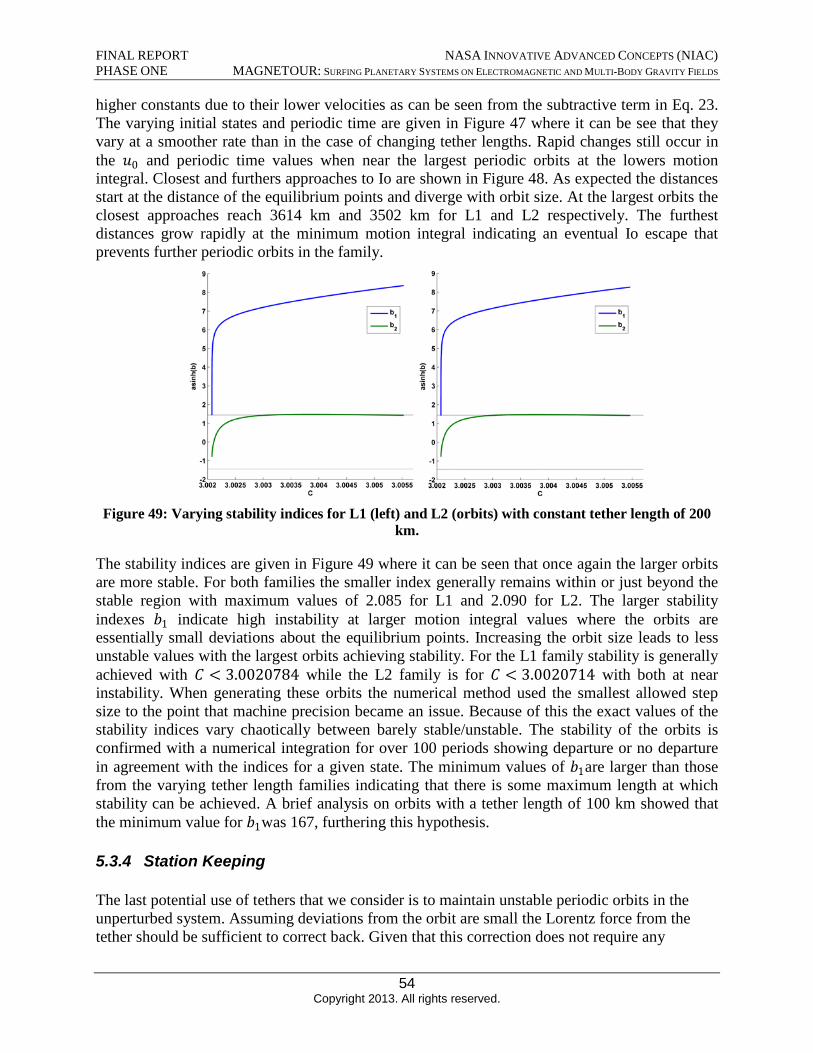
FINAL REPORT NASA INNOVATIVE ADVANCED CONCEPTS (NIAC) PHASE ONE MAGNETOUR: SURFING PLANETARY SYSTEMS ON ELECTROMAGNETIC AND MULTI-BODY GRAVITY FIELDS
higher constants due to their lower velocities as can be seen from the subtractive term in Eq. 23. The varying initial states and periodic time are given in Figure 47 where it can be see that they vary at a smoother rate than in the case of changing tether lengths. Rapid changes still occur in the u0 and periodic time values when near the largest periodic orbits at the lowers motion integral. Closest and furthers approaches to Io are shown in Figure 48. As expected the distances start at the distance of the equilibrium points and diverge with orbit size. At the largest orbits the closest approaches reach 3614 km and 3502 km for L1 and L2 respectively. The furthest distances grow rapidly at the minimum motion integral indicating an eventual Io escape that prevents further periodic orbits in the family.
Figure 49: Varying stability indices for L1 (left) and L2 (orbits) with constant tether length of 200 km.
The stability indices are given in Figure 49 where it can be seen that once again the larger orbits are more stable. For both families the smaller index generally remains within or just beyond the stable region with maximum values of 2.085 for L1 and 2.090 for L2. The larger stability indexes b1 indicate high instability at larger motion integral values where the orbits are essentially small deviations about the equilibrium points. Increasing the orbit size leads to less unstable values with the largest orbits achieving stability. For the L1 family stability is generally achieved with C < 3.0020784 while the L2 family is for C < 3.0020714 with both at near instability. When generating these orbits the numerical method used the smallest allowed step size to the point that machine precision became an issue. Because of this the exact values of the stability indices vary chaotically between barely stable/unstable. The stability of the orbits is confirmed with a numerical integration for over 100 periods showing departure or no departure in agreement with the indices for a given state. The minimum values of b1are larger than those from the varying tether length families indicating that there is some maximum length at which stability can be achieved. A brief analysis on orbits with a tether length of 100 km showed that the minimum value for b1was 167, furthering this hypothesis.
5.3.4 Station Keeping
The last potential use of tethers that we consider is to maintain unstable periodic orbits in the unperturbed system. Assuming deviations from the orbit are small the Lorentz force from the tether should be sufficient to correct back. Given that this correction does not require any
54 Copyright 2013. All rights reserved.
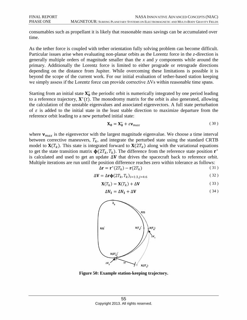
FINAL REPORT NASA INNOVATIVE ADVANCED CONCEPTS (NIAC) PHASE ONE MAGNETOUR: SURFING PLANETARY SYSTEMS ON ELECTROMAGNETIC AND MULTI-BODY GRAVITY FIELDS
consumables such as propellant it is likely that reasonable mass savings can be accumulated over time.
As the tether force is coupled with tether orientation fully solving problem can become difficult. Particular issues arise when evaluating non-planar orbits as the Lorentz force in the z-direction is generally multiple orders of magnitude smaller than the x and y components while around the primary. Additionally the Lorentz force is limited to either prograde or retrograde directions depending on the distance from Jupiter. While overcoming these limitations is possible it is beyond the scope of the current work. For our initial evaluation of tether-based station keeping we simply assess if the Lorentz force can provide corrective ΔVs within reasonable time spans.
Starting from an initial state X0∗ the periodic orbit is numerically integrated by one period leading to a reference trajectory, X∗(t). The monodromy matrix for the orbit is also generated, allowing the calculation of the unstable eigenvalues and associated eigenvectors. A full state perturbation of ε is added to the initial state in the least stable direction to maximize departure from the reference orbit leading to a new perturbed initial state:
X0 = X0∗ + ενmax ( 30 )
where νmax is the eigenvector with the largest magnitude eigenvalue. We choose a time interval between corrective maneuvers, Tk , and integrate the perturbed state using the standard CRTB model to X(Tk ). This state is integrated forward to X(2Tk ) along with the variational equations to get the state transition matrix ϕ(2Tk , Tk ). The difference from the reference state position r∗
is calculated and used to get an update ∆V that drives the spacecraft back to reference orbit. Multiple iterations are run until the position difference reaches zero within tolerance as follows:
∆r = r∗(2Tk) − r(2Tk) ( 31 )
∆V = ∆rϕ(2Tk, Tk)i=1:3,j=4:6 ( 32 )
X(Tk) = X(Tk) + ∆V ( 33 )
∆V1 = ∆V1 + ∆V ( 34 )
Figure 50: Example station-keeping trajectory.
55 Copyright 2013. All rights reserved.
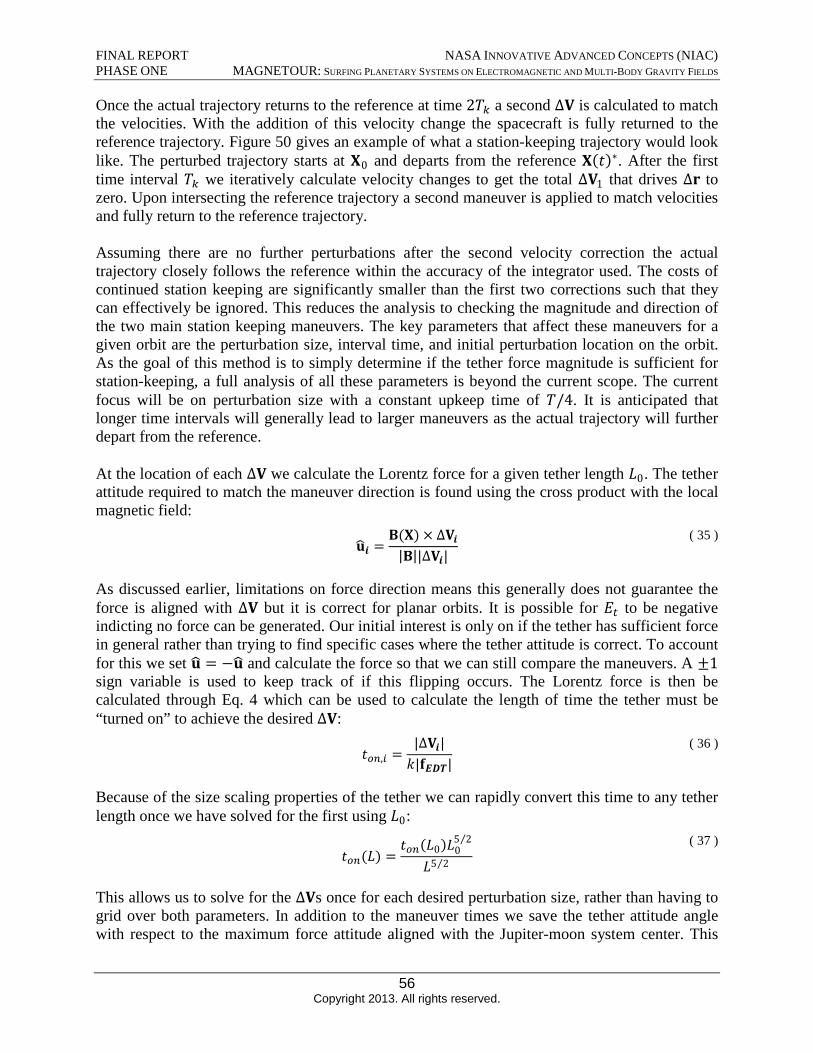
FINAL REPORT NASA INNOVATIVE ADVANCED CONCEPTS (NIAC) PHASE ONE MAGNETOUR: SURFING PLANETARY SYSTEMS ON ELECTROMAGNETIC AND MULTI-BODY GRAVITY FIELDS
Once the actual trajectory returns to the reference at time 2Tk a second ∆V is calculated to match the velocities. With the addition of this velocity change the spacecraft is fully returned to the reference trajectory. Figure 50 gives an example of what a station-keeping trajectory would look like. The perturbed trajectory starts at X0 and departs from the reference X(t)∗. After the first time interval Tk we iteratively calculate velocity changes to get the total ∆V1 that drives ∆r to zero. Upon intersecting the reference trajectory a second maneuver is applied to match velocities and fully return to the reference trajectory.
Assuming there are no further perturbations after the second velocity correction the actual trajectory closely follows the reference within the accuracy of the integrator used. The costs of continued station keeping are significantly smaller than the first two corrections such that they can effectively be ignored. This reduces the analysis to checking the magnitude and direction of the two main station keeping maneuvers. The key parameters that affect these maneuvers for a given orbit are the perturbation size, interval time, and initial perturbation location on the orbit. As the goal of this method is to simply determine if the tether force magnitude is sufficient for station-keeping, a full analysis of all these parameters is beyond the current scope. The current focus will be on perturbation size with a constant upkeep time of T/4. It is anticipated that longer time intervals will generally lead to larger maneuvers as the actual trajectory will further depart from the reference.
At the location of each ∆V we calculate the Lorentz force for a given tether length L0. The tether attitude required to match the maneuver direction is found using the cross product with the local magnetic field:
B(X) × ∆Vi ( 35 ) u =^i |B||∆Vi|
As discussed earlier, limitations on force direction means this generally does not guarantee the force is aligned with ∆V but it is correct for planar orbits. It is possible for Et to be negative indicting no force can be generated. Our initial interest is only on if the tether has sufficient force in general rather than trying to find specific cases where the tether attitude is correct. To account for this we set u = −u and calculate the force so that we can still compare the maneuvers. A ±1 sign variable is used to keep track of if this flipping occurs. The Lorentz force is then be calculated through Eq. 4 which can be used to calculate the length of time the tether must be “turned on” to achieve the desired ∆V:
|∆Vi| ( 36 ) =ton,i k|fEDT|
Because of the size scaling properties of the tether we can rapidly convert this time to any tether length once we have solved for the first using L0:
5⁄2 ( 37 ) ton (L0)L0ton (L) = L5⁄2
This allows us to solve for the ∆Vs once for each desired perturbation size, rather than having to grid over both parameters. In addition to the maneuver times we save the tether attitude angle with respect to the maximum force attitude aligned with the Jupiter-moon system center. This
56 Copyright 2013. All rights reserved.
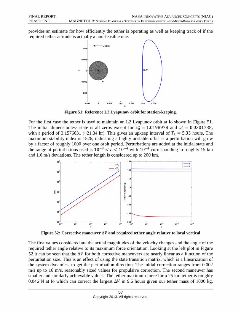
FINAL REPORT NASA INNOVATIVE ADVANCED CONCEPTS (NIAC) PHASE ONE MAGNETOUR: SURFING PLANETARY SYSTEMS ON ELECTROMAGNETIC AND MULTI-BODY GRAVITY FIELDS
provides an estimate for how efficiently the tether is operating as well as keeping track of if the required tether attitude is actually a non-feasible one.
Figure 51: Reference L2 Lyapunov orbit for station-keeping.
For the first case the tether is used to maintain an L2 Lyapunov orbit at Io shown in Figure 51. The initial dimensionless state is all zeros except for x0
∗ = 1.0198978 and v0∗ = 0.0301738,
with a period of 3.1576631 (~21.34 hr). This gives an upkeep interval of Tk = 5.33 hours. The maximum stability index is 1526, indicating a highly unstable orbit as a perturbation will grow by a factor of roughly 1000 over one orbit period. Perturbations are added at the initial state and the range of perturbations used is 10−8 < ε < 10−4 with 10−4 corresponding to roughly 15 km and 1.6 m/s deviations. The tether length is considered up to 200 km.
Figure 52: Corrective maneuver ∆V and required tether angle relative to local vertical
The first values considered are the actual magnitudes of the velocity changes and the angle of the required tether angle relative to its maximum force orientation. Looking at the left plot in Figure 52 it can be seen that the ∆V for both corrective maneuvers are nearly linear as a function of the perturbation size. This is an effect of using the state transition matrix, which is a linearization of the system dynamics, to get the perturbation direction. The initial correction ranges from 0.002 m/s up to 16 m/s, reasonably sized values for propulsive correction. The second maneuver has smaller and similarly achievable values. The tether maximum force for a 25 km tether is roughly 0.046 N at Io which can correct the largest ∆V in 9.6 hours given our tether mass of 1000 kg.
57 Copyright 2013. All rights reserved.
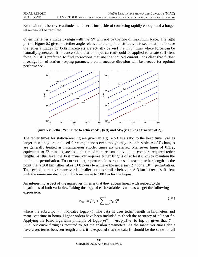
FINAL REPORT NASA INNOVATIVE ADVANCED CONCEPTS (NIAC) PHASE ONE MAGNETOUR: SURFING PLANETARY SYSTEMS ON ELECTROMAGNETIC AND MULTI-BODY GRAVITY FIELDS
Even with this best case attitude the tether is incapable of correcting rapidly enough and a longer tether would be required.
Often the tether attitude to align with the ∆V will not be the one of maximum force. The right plot of Figure 52 gives the tether angle relative to the optimal attitude. It is seen that in this case the tether attitudes for both maneuvers are actually beyond the ±90° lines where force can be naturally generated. It is conceivable that an input current could be applied to create sufficient force, but it is preferred to find corrections that use the induced current. It is clear that further investigation of station-keeping parameters on maneuver direction will be needed for optimal performance.
Figure 53: Tether “on” time to achieve ∆V1 (left) and ∆V2 (right) as a fraction of Tk.
The tether times for station-keeping are given in Figure 53 as a ratio to the keep time. Values larger than unity are included for completeness even though they are infeasible. As ∆V changes are generally treated as instantaneous shorter times are preferred. Maneuver times of 0.1Tk , equivalent to 32 minutes, are used as a maximum reasonable value to compare required tether lengths. At this level the first maneuver requires tether lengths of at least 6 km to maintain the minimum perturbation. To correct larger perturbations requires increasing tether length to the point that a 200 km tether takes 1.08 hours to achieve the necessary ∆V for a 10−4 perturbation. The second corrective maneuver is smaller but has similar behavior. A 3 km tether is sufficient with the minimum deviation which increases to 100 km for the largest.
An interesting aspect of the maneuver times is that they appear linear with respect to the logarithms of both variables. Taking the log10 of each variable as well as we get the following expression:
4 ( 38 ) = βLl + Σ τmεlmton,l
m=0
where the subscript (∗)l indicates log10(∗). The data fit uses tether length in kilometers and maneuver time in hours. Higher orders have been included to check the accuracy of a linear fit. Applying the basic logarithm principle of log10(mn) = nlog10(m) to Eq. 37 gives that β = −2.5 but curve fitting is required to get the epsilon parameters. As the maneuver times don’thave cross terms between length and ε it is expected that the data fit should be the same for all
58 Copyright 2013. All rights reserved.
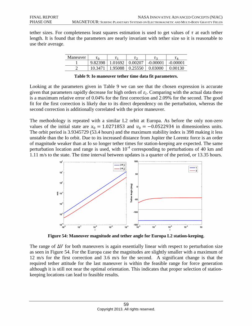
FINAL REPORT NASA INNOVATIVE ADVANCED CONCEPTS (NIAC) PHASE ONE MAGNETOUR: SURFING PLANETARY SYSTEMS ON ELECTROMAGNETIC AND MULTI-BODY GRAVITY FIELDS
tether sizes. For completeness least squares estimation is used to get values of τ at each tether length. It is found that the parameters are nearly invariant with tether size so it is reasonable to use their average.
Maneuver τ0 τ1 τ2 τ3 τ41 9.82398 1.01692 0.00207 -0.00001 -0.000012 10.3471 1.95088 0.25550 0.03000 0.00130
Table 9: Io maneuver tether time data fit parameters.
Looking at the parameters given in Table 9 we can see that the chosen expression is accurate given that parameters rapidly decrease for high orders of εl. Comparing with the actual data there is a maximum relative error of 0.04% for the first correction and 2.09% for the second. The good fit for the first correction is likely due to its direct dependency on the perturbation, whereas the second correction is additionally correlated with the prior maneuver.
The methodology is repeated with a similar L2 orbit at Europa. As before the only non-zero values of the initial state are x0 = 1.0271853 and v0 = −0.0522934 in dimensionless units. The orbit period is 3.9345729 (53.4 hours) and the maximum stability index is 398 making it less unstable than the Io orbit. Due to its increased distance from Jupiter the Lorentz force is an order of magnitude weaker than at Io so longer tether times for station-keeping are expected. The same perturbation location and range is used, with 10-4 corresponding to perturbations of 40 km and 1.11 m/s to the state. The time interval between updates is a quarter of the period, or 13.35 hours.
Figure 54: Maneuver magnitude and tether angle for Europa L2 station-keeping.
The range of ∆V for both maneuvers is again essentially linear with respect to perturbation size as seen in Figure 54. For the Europa case the magnitudes are slightly smaller with a maximum of 12 m/s for the first correction and 3.6 m/s for the second. A significant change is that the required tether attitude for the last maneuver is within the feasible range for force generation although it is still not near the optimal orientation. This indicates that proper selection of station-keeping locations can lead to feasible results.
59 Copyright 2013. All rights reserved.
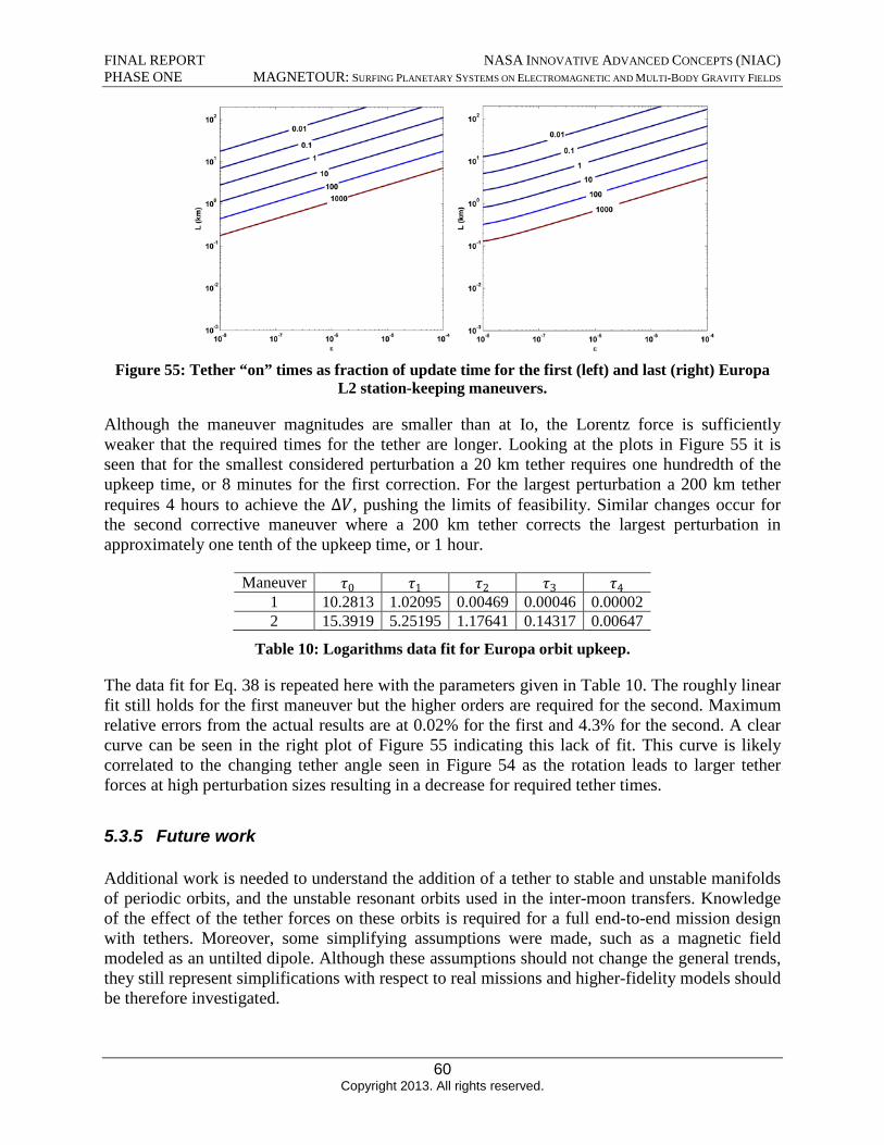
FINAL REPORT NASA INNOVATIVE ADVANCED CONCEPTS (NIAC) PHASE ONE MAGNETOUR: SURFING PLANETARY SYSTEMS ON ELECTROMAGNETIC AND MULTI-BODY GRAVITY FIELDS
Figure 55: Tether “on” times as fraction of update time for the first (left) and last (right) Europa L2 station-keeping maneuvers.
Although the maneuver magnitudes are smaller than at Io, the Lorentz force is sufficiently weaker that the required times for the tether are longer. Looking at the plots in Figure 55 it is seen that for the smallest considered perturbation a 20 km tether requires one hundredth of the upkeep time, or 8 minutes for the first correction. For the largest perturbation a 200 km tether requires 4 hours to achieve the ∆V, pushing the limits of feasibility. Similar changes occur for the second corrective maneuver where a 200 km tether corrects the largest perturbation in approximately one tenth of the upkeep time, or 1 hour.
Maneuver τ0 τ1 τ2 τ3 τ41 10.2813 1.02095 0.00469 0.00046 0.00002 2 15.3919 5.25195 1.17641 0.14317 0.00647
Table 10: Logarithms data fit for Europa orbit upkeep.
The data fit for Eq. 38 is repeated here with the parameters given in Table 10. The roughly linear fit still holds for the first maneuver but the higher orders are required for the second. Maximum relative errors from the actual results are at 0.02% for the first and 4.3% for the second. A clear curve can be seen in the right plot of Figure 55 indicating this lack of fit. This curve is likely correlated to the changing tether angle seen in Figure 54 as the rotation leads to larger tether forces at high perturbation sizes resulting in a decrease for required tether times.
5.3.5 Future work
Additional work is needed to understand the addition of a tether to stable and unstable manifolds of periodic orbits, and the unstable resonant orbits used in the inter-moon transfers. Knowledge of the effect of the tether forces on these orbits is required for a full end-to-end mission design with tethers. Moreover, some simplifying assumptions were made, such as a magnetic field modeled as an untilted dipole. Although these assumptions should not change the general trends, they still represent simplifications with respect to real missions and higher-fidelity models should be therefore investigated.
60 Copyright 2013. All rights reserved.
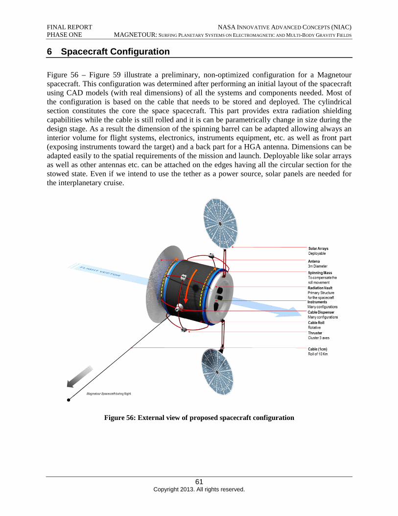
FINAL REPORT NASA INNOVATIVE ADVANCED CONCEPTS (NIAC) PHASE ONE MAGNETOUR: SURFING PLANETARY SYSTEMS ON ELECTROMAGNETIC AND MULTI-BODY GRAVITY FIELDS
6 Spacecraft Configuration
Figure 56 – Figure 59 illustrate a preliminary, non-optimized configuration for a Magnetour spacecraft. This configuration was determined after performing an initial layout of the spacecraft using CAD models (with real dimensions) of all the systems and components needed. Most of the configuration is based on the cable that needs to be stored and deployed. The cylindrical section constitutes the core the space spacecraft. This part provides extra radiation shielding capabilities while the cable is still rolled and it is can be parametrically change in size during the design stage. As a result the dimension of the spinning barrel can be adapted allowing always an interior volume for flight systems, electronics, instruments equipment, etc. as well as front part (exposing instruments toward the target) and a back part for a HGA antenna. Dimensions can be adapted easily to the spatial requirements of the mission and launch. Deployable like solar arrays as well as other antennas etc. can be attached on the edges having all the circular section for the stowed state. Even if we intend to use the tether as a power source, solar panels are needed for the interplanetary cruise.
Figure 56: External view of proposed spacecraft configuration
61 Copyright 2013. All rights reserved.
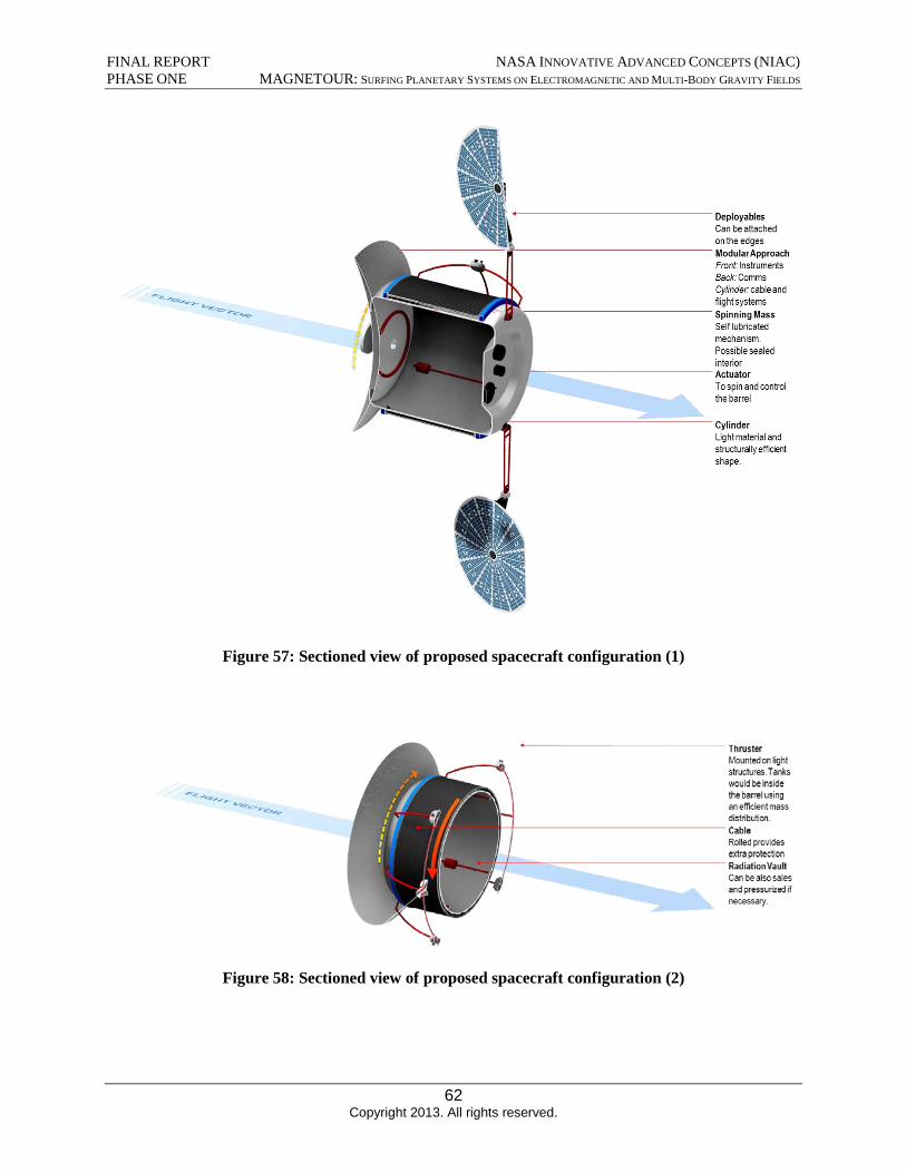
FINAL REPORT NASA INNOVATIVE ADVANCED CONCEPTS (NIAC) PHASE ONE MAGNETOUR: SURFING PLANETARY SYSTEMS ON ELECTROMAGNETIC AND MULTI-BODY GRAVITY FIELDS
Figure 57: Sectioned view of proposed spacecraft configuration (1)
Figure 58: Sectioned view of proposed spacecraft configuration (2)
62 Copyright 2013. All rights reserved.
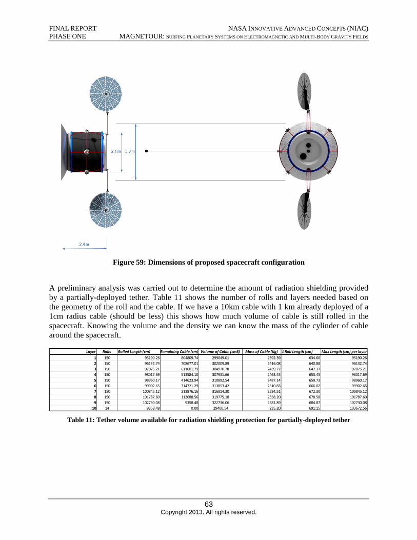
Layer Rolls Rolled Length (cm) Remaining Cable (cm) Volume of Cable (cm3) Mass of Cable (Kg) 1 Roll Length (cm) Max Length (cm) per layer 1 150 95190.26 804809.74 299049.01 2392.39 634.60 95190.26 2 150 96132.74 708677.01 302009.89 2416.08 640.88 96132.74 3 150 97075.21 611601.79 304970.78 2439.77 647.17 97075.21 4 150 98017.69 513584.10 307931.66 2463.45 653.45 98017.69 5 150 98960.17 414623.94 310892.54 2487.14 659.73 98960.17 6 150 99902.65 314721.29 313853.42 2510.83 666.02 99902.65 7 150 100845.12 213876.16 316814.30 2534.51 672.30 100845.12 8 150 101787.60 112088.56 319775.18 2558.20 678.58 101787.60 9 150 102730.08 9358.48 322736.06 2581.89 684.87 102730.08
10 14 9358.48 0.00 29400.54 235.20 691.15 103672.56
FINAL REPORT NASA INNOVATIVE ADVANCED CONCEPTS (NIAC) PHASE ONE MAGNETOUR: SURFING PLANETARY SYSTEMS ON ELECTROMAGNETIC AND MULTI-BODY GRAVITY FIELDS
Figure 59: Dimensions of proposed spacecraft configuration
A preliminary analysis was carried out to determine the amount of radiation shielding provided by a partially-deployed tether. Table 11 shows the number of rolls and layers needed based on the geometry of the roll and the cable. If we have a 10km cable with 1 km already deployed of a 1cm radius cable (should be less) this shows how much volume of cable is still rolled in the spacecraft. Knowing the volume and the density we can know the mass of the cylinder of cable around the spacecraft.
Table 11: Tether volume available for radiation shielding protection for partially-deployed tether
63 Copyright 2013. All rights reserved.

FINAL REPORT NASA INNOVATIVE ADVANCED CONCEPTS (NIAC) PHASE ONE MAGNETOUR: SURFING PLANETARY SYSTEMS ON ELECTROMAGNETIC AND MULTI-BODY GRAVITY FIELDS
7 Jovian Mission Design
7.1 Mission Overview
Magnetour is particularly promising in the Jovian system where the magnetic field is rotating rapidly and is exceptionally strong. We then perform a preliminary mission design analysis at Jupiter using simplified models for the gravitational and magnetic fields. The trajectory phases are the following:
0. Interplanetary (not the focus of this study)1. Capture2. Apojove Pump Down3. Perijove Pump Up4. InterMoon Superhighway (low-energy tour)
In this Phase 1 project, the options for each of the trajectory phases above were considered. The Magnetour propulsive capability is notably different from conventional spacecraft, making the tour design a new and challenging area of research. The delta-v necessary to achieve a long planetary moon tour is achievable with the Magnetour concept thru three fundamental sources, 1) tether 2) gravity assist moon flybys, and 3) non-tether propulsive capabilities. The latter two are typical in conventional tours, while the tether option is the novel addition of the Magnetour concept. Ideally, a complete propellantless mission is possible, although in practice a small propulsive capability such as an attitude control engine will likely accompany the spacecraft and can also be used for minor translational control. Therefore all three of the delta-v options are considered. In this Phase 1 project, trade studies were performed considering conventional wisdom of a typical moon tour combined with the added complexity of a propellantless thrust originating with the tether. Fundamentally the trade studies stem from the following attributes:
• Time efficiency for maneuvers using the tether increases with smaller distances toJupiter.
• Radiation dose increases with smaller distances to Jupiter.• The tether can lower apojove with thrusting near perijove (where tether is most efficient).• The tether can raise perijove, with thrusting near apojove (where tether is least efficient).
Several of these attributes are conflicting and lead to classic trade-offs for the design process in terms of radiation dose, time of flight, propellant cost (in cases where low- or high- thrust engines supplement the solutions) and science potential at each of the moons. Based on this Phase 1 study, the following is a summary of the suggested trajectory solutions for further study in Phase 2: Solution strategies:
1. Capture:a. Tether only (see section 7.3.1); orb. Tether plus flybys prior to JOI (see section 7.3.2)
2. Apojove Pump Down:a. Tether only (see section 7.3.1); or
64 Copyright 2013. All rights reserved.
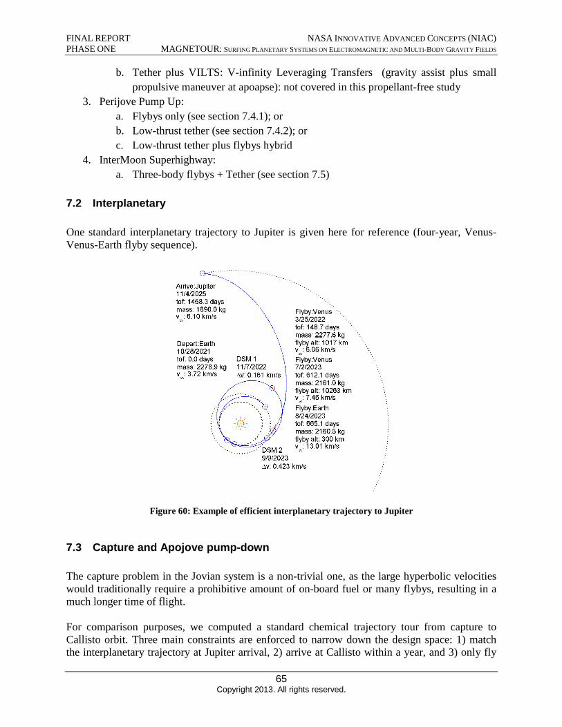
FINAL REPORT NASA INNOVATIVE ADVANCED CONCEPTS (NIAC) PHASE ONE MAGNETOUR: SURFING PLANETARY SYSTEMS ON ELECTROMAGNETIC AND MULTI-BODY GRAVITY FIELDS
b. Tether plus VILTS: V-infinity Leveraging Transfers (gravity assist plus smallpropulsive maneuver at apoapse): not covered in this propellant-free study
3. Perijove Pump Up:a. Flybys only (see section 7.4.1); orb. Low-thrust tether (see section 7.4.2); orc. Low-thrust tether plus flybys hybrid
4. InterMoon Superhighway:a. Three-body flybys + Tether (see section 7.5)
7.2 Interplanetary
One standard interplanetary trajectory to Jupiter is given here for reference (four-year, Venus-Venus-Earth flyby sequence).
Figure 60: Example of efficient interplanetary trajectory to Jupiter
7.3 Capture and Apojove pump-down
The capture problem in the Jovian system is a non-trivial one, as the large hyperbolic velocities would traditionally require a prohibitive amount of on-board fuel or many flybys, resulting in a much longer time of flight.
For comparison purposes, we computed a standard chemical trajectory tour from capture to Callisto orbit. Three main constraints are enforced to narrow down the design space: 1) match the interplanetary trajectory at Jupiter arrival, 2) arrive at Callisto within a year, and 3) only fly
65 Copyright 2013. All rights reserved.
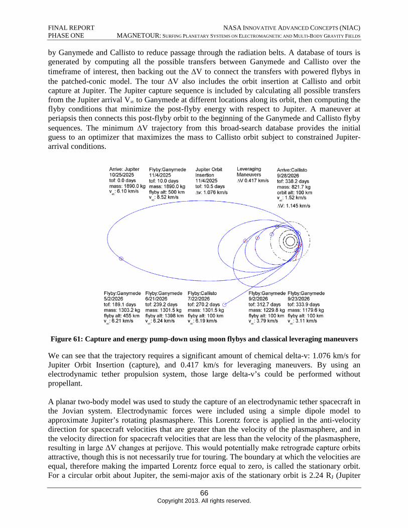
FINAL REPORT NASA INNOVATIVE ADVANCED CONCEPTS (NIAC) PHASE ONE MAGNETOUR: SURFING PLANETARY SYSTEMS ON ELECTROMAGNETIC AND MULTI-BODY GRAVITY FIELDS
by Ganymede and Callisto to reduce passage through the radiation belts. A database of tours is generated by computing all the possible transfers between Ganymede and Callisto over the timeframe of interest, then backing out the ΔV to connect the transfers with powered flybys in the patched-conic model. The tour ΔV also includes the orbit insertion at Callisto and orbit capture at Jupiter. The Jupiter capture sequence is included by calculating all possible transfers from the Jupiter arrival V∞ to Ganymede at different locations along its orbit, then computing the flyby conditions that minimize the post-flyby energy with respect to Jupiter. A maneuver at periapsis then connects this post-flyby orbit to the beginning of the Ganymede and Callisto flyby sequences. The minimum ΔV trajectory from this broad-search database provides the initial guess to an optimizer that maximizes the mass to Callisto orbit subject to constrained Jupiter-arrival conditions.
Figure 61: Capture and energy pump-down using moon flybys and classical leveraging maneuvers
We can see that the trajectory requires a significant amount of chemical delta-v: 1.076 km/s for Jupiter Orbit Insertion (capture), and 0.417 km/s for leveraging maneuvers. By using an electrodynamic tether propulsion system, those large delta-v’s could be performed without propellant.
A planar two-body model was used to study the capture of an electrodynamic tether spacecraft in the Jovian system. Electrodynamic forces were included using a simple dipole model to approximate Jupiter’s rotating plasmasphere. This Lorentz force is applied in the anti-velocity direction for spacecraft velocities that are greater than the velocity of the plasmasphere, and in the velocity direction for spacecraft velocities that are less than the velocity of the plasmasphere, resulting in large ΔV changes at perijove. This would potentially make retrograde capture orbits attractive, though this is not necessarily true for touring. The boundary at which the velocities are equal, therefore making the imparted Lorentz force equal to zero, is called the stationary orbit. For a circular orbit about Jupiter, the semi-major axis of the stationary orbit is 2.24 RJ (Jupiter
66 Copyright 2013. All rights reserved.
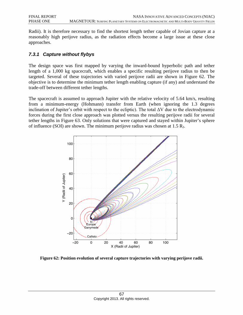
FINAL REPORT NASA INNOVATIVE ADVANCED CONCEPTS (NIAC) PHASE ONE MAGNETOUR: SURFING PLANETARY SYSTEMS ON ELECTROMAGNETIC AND MULTI-BODY GRAVITY FIELDS
Radii). It is therefore necessary to find the shortest length tether capable of Jovian capture at a reasonably high perijove radius, as the radiation effects become a large issue at these close approaches.
7.3.1 Capture without flybys
The design space was first mapped by varying the inward-bound hyperbolic path and tether length of a 1,000 kg spacecraft, which enables a specific resulting perijove radius to then be targeted. Several of these trajectories with varied perijove radii are shown in Figure 62. The objective is to determine the minimum tether length enabling capture (if any) and understand the trade-off between different tether lengths.
The spacecraft is assumed to approach Jupiter with the relative velocity of 5.64 km/s, resulting from a minimum-energy (Hohmann) transfer from Earth (when ignoring the 1.3 degrees inclination of Jupiter’s orbit with respect to the ecliptic). The total ΔV due to the electrodynamic forces during the first close approach was plotted versus the resulting perijove radii for several tether lengths in Figure 63. Only solutions that were captured and stayed within Jupiter’s sphere of influence (SOI) are shown. The minimum perijove radius was chosen at 1.5 RJ.
Figure 62: Position evolution of several capture trajectories with varying perijove radii.
67 Copyright 2013. All rights reserved.
GanymedeEuropa
Io
Callisto
−20 0 20 80 100
−20
0
20
40
60
80
100
40 60X (Radii of Jupiter)
Y (R
adii
of J
upite
r)
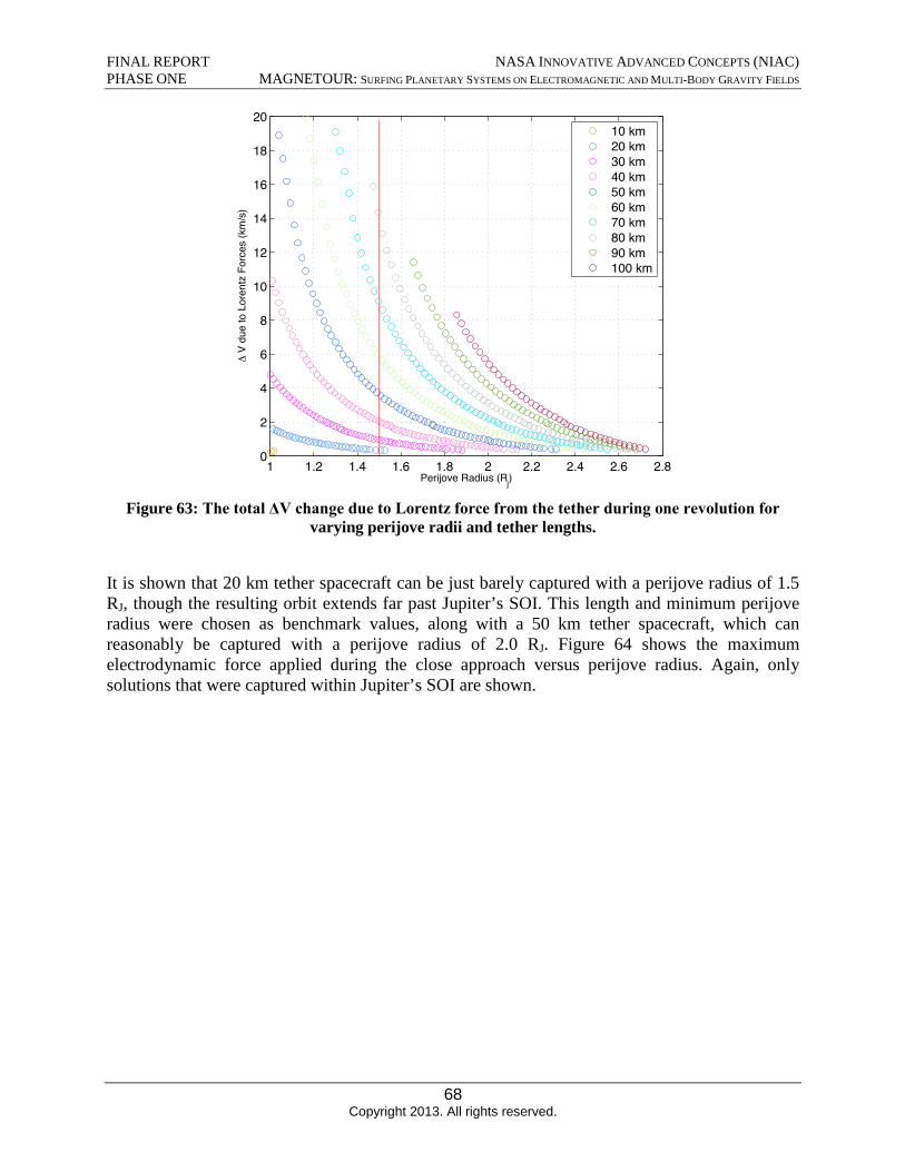
FINAL REPORT NASA INNOVATIVE ADVANCED CONCEPTS (NIAC) PHASE ONE MAGNETOUR: SURFING PLANETARY SYSTEMS ON ELECTROMAGNETIC AND MULTI-BODY GRAVITY FIELDS
Figure 63: The total ΔV change due to Lorentz force from the tether during one revolution for varying perijove radii and tether lengths.
It is shown that 20 km tether spacecraft can be just barely captured with a perijove radius of 1.5 RJ, though the resulting orbit extends far past Jupiter’s SOI. This length and minimum perijove radius were chosen as benchmark values, along with a 50 km tether spacecraft, which can reasonably be captured with a perijove radius of 2.0 RJ. Figure 64 shows the maximum electrodynamic force applied during the close approach versus perijove radius. Again, only solutions that were captured within Jupiter’s SOI are shown.
68 Copyright 2013. All rights reserved.
1 1.2 1.4 1.6 1.8 2 2.2 2.4 2.6 2.8
2
4
6
8
10
12
14
16
18
20
Perijove Radius (Rj)
∆ V
due
to L
oren
tz F
orce
s (k
m/s
)
0
10 km20 km30 km40 km50 km60 km70 km80 km90 km100 km
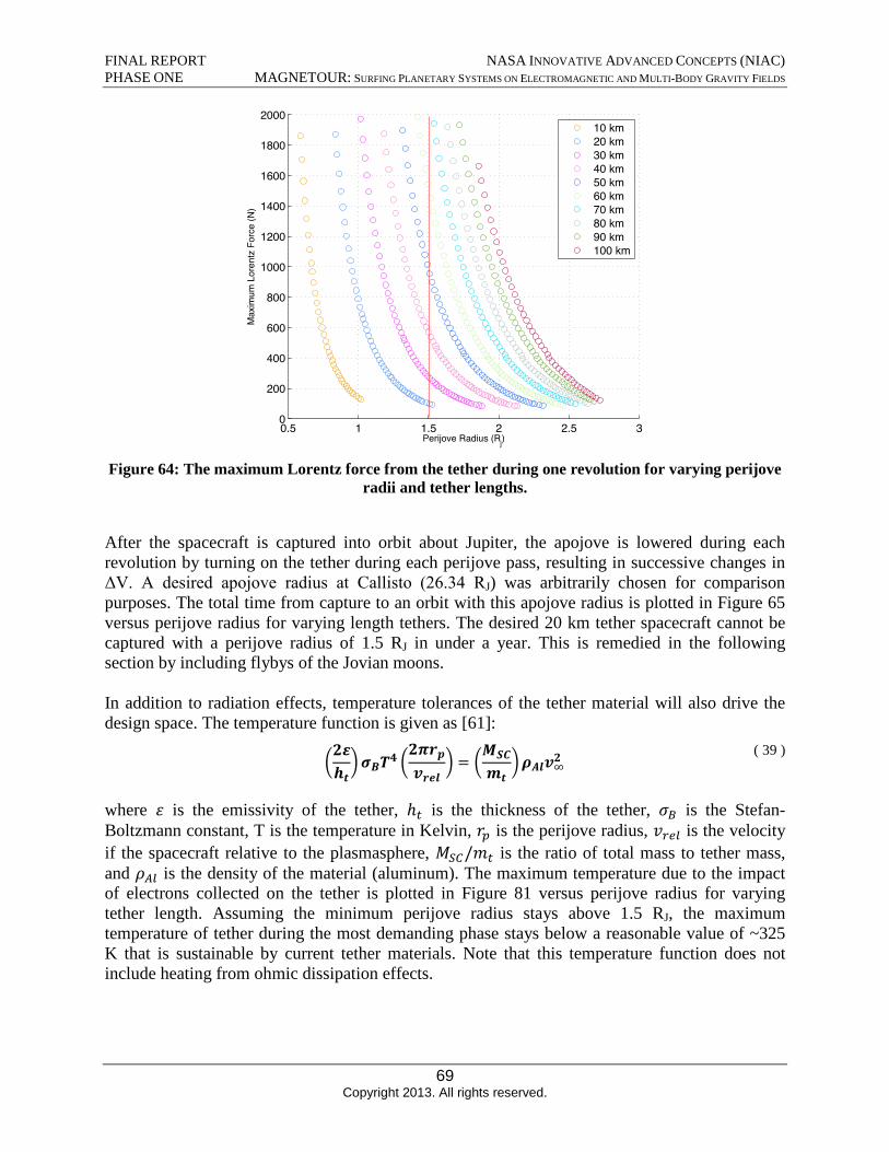
FINAL REPORT NASA INNOVATIVE ADVANCED CONCEPTS (NIAC) PHASE ONE MAGNETOUR: SURFING PLANETARY SYSTEMS ON ELECTROMAGNETIC AND MULTI-BODY GRAVITY FIELDS
Figure 64: The maximum Lorentz force from the tether during one revolution for varying perijove radii and tether lengths.
After the spacecraft is captured into orbit about Jupiter, the apojove is lowered during each revolution by turning on the tether during each perijove pass, resulting in successive changes in ΔV. A desired apojove radius at Callisto (26.34 RJ) was arbitrarily chosen for comparison purposes. The total time from capture to an orbit with this apojove radius is plotted in Figure 65 versus perijove radius for varying length tethers. The desired 20 km tether spacecraft cannot be captured with a perijove radius of 1.5 RJ in under a year. This is remedied in the following section by including flybys of the Jovian moons.
In addition to radiation effects, temperature tolerances of the tether material will also drive the design space. The temperature function is given as [61]:
(2ε 2πrp) = (
MSC ( 39 ) ) σBT4 ( ) ρAlv∞
2
ht vrel mt
where ε is the emissivity of the tether, ht is the thickness of the tether, σB is the Stefan-Boltzmann constant, T is the temperature in Kelvin, rp is the perijove radius, vrel is the velocity if the spacecraft relative to the plasmasphere, MSC /mt is the ratio of total mass to tether mass, and ρAl is the density of the material (aluminum). The maximum temperature due to the impact of electrons collected on the tether is plotted in Figure 81 versus perijove radius for varying tether length. Assuming the minimum perijove radius stays above 1.5 RJ, the maximum temperature of tether during the most demanding phase stays below a reasonable value of ~325 K that is sustainable by current tether materials. Note that this temperature function does not include heating from ohmic dissipation effects.
69 Copyright 2013. All rights reserved.
0.5 1 1.5 2 2.5 3
200
400
600
800
1000
1200
1400
1600
1800
2000
Perijove Radius (Rj)
Max
imum
Lor
entz
For
ce (N
)
0
10 km20 km30 km40 km50 km60 km70 km80 km90 km100 km
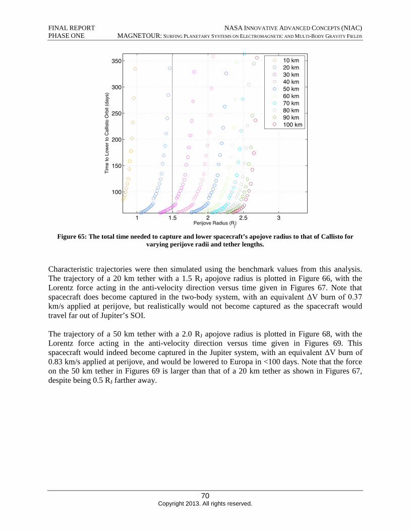
FINAL REPORT NASA INNOVATIVE ADVANCED CONCEPTS (NIAC) PHASE ONE MAGNETOUR: SURFING PLANETARY SYSTEMS ON ELECTROMAGNETIC AND MULTI-BODY GRAVITY FIELDS
Figure 65: The total time needed to capture and lower spacecraft’s apojove radius to that of Callisto for varying perijove radii and tether lengths.
Characteristic trajectories were then simulated using the benchmark values from this analysis. The trajectory of a 20 km tether with a 1.5 RJ apojove radius is plotted in Figure 66, with the Lorentz force acting in the anti-velocity direction versus time given in Figures 67. Note that spacecraft does become captured in the two-body system, with an equivalent ΔV burn of 0.37 km/s applied at perijove, but realistically would not become captured as the spacecraft would travel far out of Jupiter’s SOI.
The trajectory of a 50 km tether with a 2.0 RJ apojove radius is plotted in Figure 68, with the Lorentz force acting in the anti-velocity direction versus time given in Figures 69. This spacecraft would indeed become captured in the Jupiter system, with an equivalent ΔV burn of 0.83 km/s applied at perijove, and would be lowered to Europa in <100 days. Note that the force on the 50 km tether in Figures 69 is larger than that of a 20 km tether as shown in Figures 67, despite being 0.5 RJ farther away.
70 Copyright 2013. All rights reserved.
1 1.5 2 2.5 3
100
150
200
250
300
350
Perijove Radius (Rj)
Tim
e to
Low
er to
Cal
listo
Orb
it (d
ays)
10 km20 km30 km40 km50 km60 km70 km80 km90 km100 km
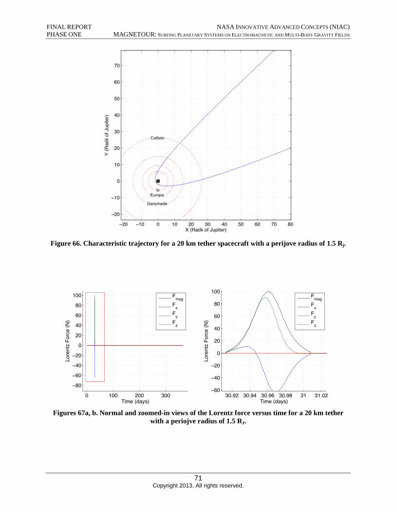
FINAL REPORT NASA INNOVATIVE ADVANCED CONCEPTS (NIAC) PHASE ONE MAGNETOUR: SURFING PLANETARY SYSTEMS ON ELECTROMAGNETIC AND MULTI-BODY GRAVITY FIELDS
Figure 66. Characteristic trajectory for a 20 km tether spacecraft with a perijove radius of 1.5 Rj.
Figures 67a, b. Normal and zoomed-in views of the Lorentz force versus time for a 20 km tether with a periojve radius of 1.5 RJ.
71 Copyright 2013. All rights reserved.
Callisto
Ganymede
EuropaIo
−20 −10 0 10 50 60 70 80
−10
−20
0
10
20
30
40
50
60
70
20 30 40X (Radii of Jupiter)
Y (R
adii
of J
upite
r)
0 100 200 300
−20
−40
−60
−80
0
20
40
60
80
100
Time (days)
Lore
ntz
Forc
e (N
)
FmagFxFyFz
30.92 30.94 30.96 30.98 31 31.02
−20
−40
−60
0
20
40
60
80
100
Time (days)
Lore
ntz
Forc
e (N
)
FmagFxFyFz
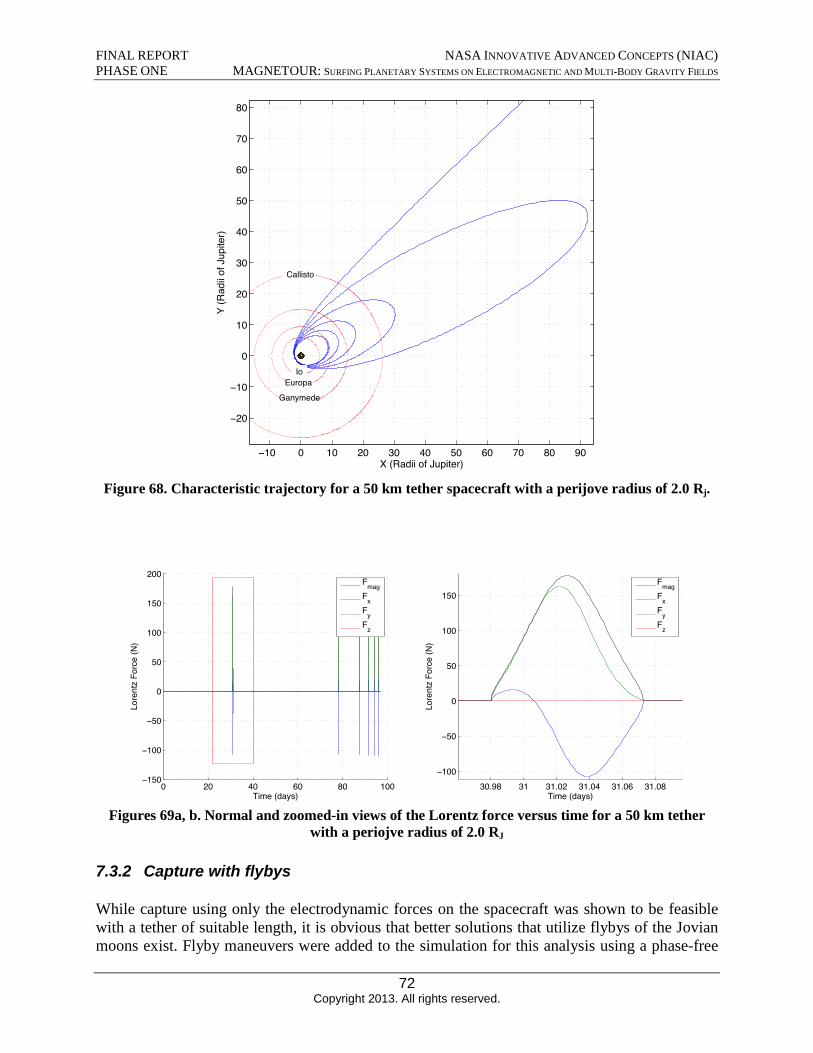
FINAL REPORT NASA INNOVATIVE ADVANCED CONCEPTS (NIAC) PHASE ONE MAGNETOUR: SURFING PLANETARY SYSTEMS ON ELECTROMAGNETIC AND MULTI-BODY GRAVITY FIELDS
Figure 68. Characteristic trajectory for a 50 km tether spacecraft with a perijove radius of 2.0 Rj.
Figures 69a, b. Normal and zoomed-in views of the Lorentz force versus time for a 50 km tether with a periojve radius of 2.0 RJ
7.3.2 Capture with flybys
While capture using only the electrodynamic forces on the spacecraft was shown to be feasible with a tether of suitable length, it is obvious that better solutions that utilize flybys of the Jovian moons exist. Flyby maneuvers were added to the simulation for this analysis using a phase-free
72 Copyright 2013. All rights reserved.
Callisto
Ganymede
IoEuropa
−10 0 10 20 60 70 80 90
−10
−20
0
10
20
30
40
50
60
70
80
30 40 50X (Radii of Jupiter)
Y (R
adii
of J
upite
r)
0 20 40 60 80 100
−100
−150
−50
0
50
100
150
200
Time (days)
Lore
ntz
Forc
e (N
)
FmagFxFyFz
30.98 31 31.02 31.04 31.06 31.08−100
−50
0
50
100
150
Time (days)
Lore
ntz
Forc
e (N
)
FmagFxFyFz
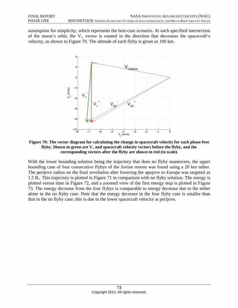
FINAL REPORT NASA INNOVATIVE ADVANCED CONCEPTS (NIAC) PHASE ONE MAGNETOUR: SURFING PLANETARY SYSTEMS ON ELECTROMAGNETIC AND MULTI-BODY GRAVITY FIELDS
assumption for simplicity, which represents the best-case scenario. At each specified intersection of the moon’s orbit, the V∞ vector is rotated in the direction that decreases the spacecraft’s velocity, as shown in Figure 70. The altitude of each flyby is given as 100 km.
Figure 70: The vector diagram for calculating the change in spacecraft velocity for each phase-free flyby. Shown in green are V∞ and spacecraft velocity vectors before the flyby, and the
corresponding vectors after the flyby are shown in red (to scale).
With the lower bounding solution being the trajectory that does no flyby maneuvers, the upper bounding case of four consecutive flybys of the Jovian moons was found using a 20 km tether. The perijove radius on the final revolution after lowering the apojove to Europa was targeted as 1.5 RJ. This trajectory is plotted in Figure 71 in comparison with no flyby solution. The energy is plotted versus time in Figure 72, and a zoomed view of the first energy step is plotted in Figure 73. The energy decrease from the four flybys is comparable to energy decrease due to the tetheralone in the no flyby case. Note that the energy decrease in the four flyby case is smaller thanthat in the no flyby case; this is due to the lower spacecraft velocity at perijove.
73 Copyright 2013. All rights reserved.
−10−8 −7 −6 −5 −4 −3 −2 −1 0
−2
−4
−6
−8
0
2
4
Vx (km/s)
V y (km
/s)
VCallisto
VSC
-VSC
+
V∞
-
V∞
+
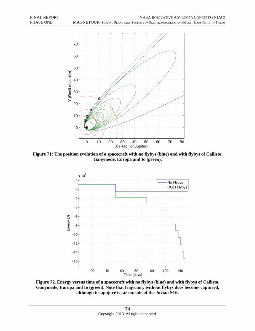
FINAL REPORT NASA INNOVATIVE ADVANCED CONCEPTS (NIAC) PHASE ONE MAGNETOUR: SURFING PLANETARY SYSTEMS ON ELECTROMAGNETIC AND MULTI-BODY GRAVITY FIELDS
Figure 71: The position evolution of a spacecraft with no flybys (blue) and with flybys of Callisto, Ganymede, Europa and Io (green).
Figure 72. Energy versus time of a spacecraft with no flybys (blue) and with flybys of Callisto, Ganymede, Europa and Io (green). Note that trajectory without flybys does become captured,
although its apojove is far outside of the Jovian SOI.
74 Copyright 2013. All rights reserved.
0 10 20 60 70 80
0
10
20
30
40
50
60
70
30 40 50X (Radii of Jupiter)
Y (R
adii
of J
upite
r)
20 40 60 80 100 120 140
−10
−12
−14
−16
−2
−4
−6
−8
0
2x 10⁷
Ener
gy (J
)
Time (days)
No FlybysCGEI Flybys
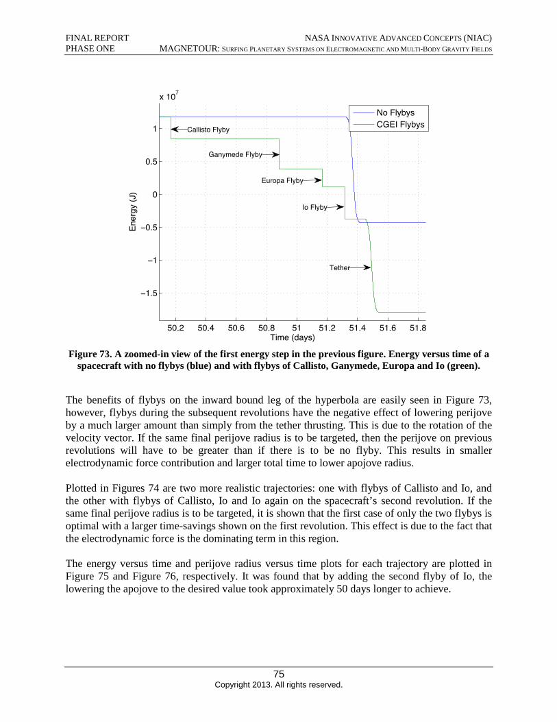
FINAL REPORT NASA INNOVATIVE ADVANCED CONCEPTS (NIAC) PHASE ONE MAGNETOUR: SURFING PLANETARY SYSTEMS ON ELECTROMAGNETIC AND MULTI-BODY GRAVITY FIELDS
Figure 73. A zoomed-in view of the first energy step in the previous figure. Energy versus time of a spacecraft with no flybys (blue) and with flybys of Callisto, Ganymede, Europa and Io (green).
The benefits of flybys on the inward bound leg of the hyperbola are easily seen in Figure 73, however, flybys during the subsequent revolutions have the negative effect of lowering perijove by a much larger amount than simply from the tether thrusting. This is due to the rotation of the velocity vector. If the same final perijove radius is to be targeted, then the perijove on previous revolutions will have to be greater than if there is to be no flyby. This results in smaller electrodynamic force contribution and larger total time to lower apojove radius.
Plotted in Figures 74 are two more realistic trajectories: one with flybys of Callisto and Io, and the other with flybys of Callisto, Io and Io again on the spacecraft’s second revolution. If the same final perijove radius is to be targeted, it is shown that the first case of only the two flybys is optimal with a larger time-savings shown on the first revolution. This effect is due to the fact that the electrodynamic force is the dominating term in this region.
The energy versus time and perijove radius versus time plots for each trajectory are plotted in Figure 75 and Figure 76, respectively. It was found that by adding the second flyby of Io, the lowering the apojove to the desired value took approximately 50 days longer to achieve.
75 Copyright 2013. All rights reserved.
50.2 50.4 50.6 50.8 51 51.2 51.4 51.6 51.8
−0.5
−1
−1.5
0
0.5
1
x 107
Ener
gy (J
)
Time (days)
No FlybysCGEI FlybysCallisto Flyby
Ganymede Flyby
Europa Flyby
Io Flyby
Tether
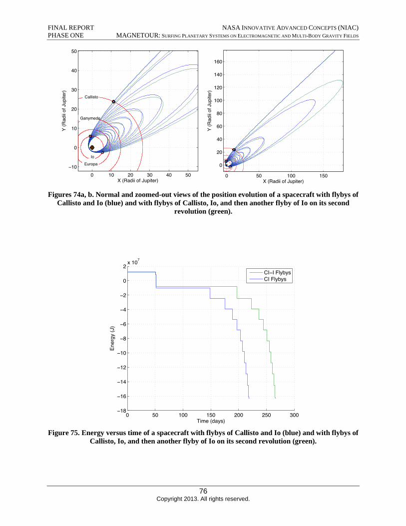
FINAL REPORT NASA INNOVATIVE ADVANCED CONCEPTS (NIAC) PHASE ONE MAGNETOUR: SURFING PLANETARY SYSTEMS ON ELECTROMAGNETIC AND MULTI-BODY GRAVITY FIELDS
Figures 74a, b. Normal and zoomed-out views of the position evolution of a spacecraft with flybys of Callisto and Io (blue) and with flybys of Callisto, Io, and then another flyby of Io on its second
revolution (green).
Figure 75. Energy versus time of a spacecraft with flybys of Callisto and Io (blue) and with flybys of Callisto, Io, and then another flyby of Io on its second revolution (green).
76 Copyright 2013. All rights reserved.
0 50 150
0
20
40
60
80
100
120
140
160
100X (Radii of Jupiter)
Y (R
adii
of J
upite
r)
0 10 40 50−10
0
10
20
30
40
50
20 30X (Radii of Jupiter)
Y (R
adii
of J
upite
r)
Ganymede
IoEuropa
Callisto
−10
−12
−14
−16
−180 50 100 150 200 250 300
−2
−4
−6
−8
0
2x 10⁷
Ener
gy (J
)
Time (days)
CI−I FlybysCI Flybys
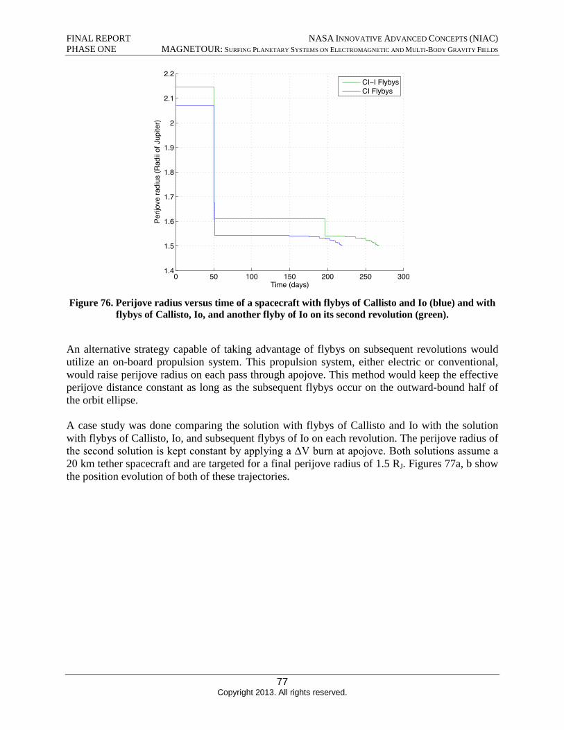
FINAL REPORT NASA INNOVATIVE ADVANCED CONCEPTS (NIAC) PHASE ONE MAGNETOUR: SURFING PLANETARY SYSTEMS ON ELECTROMAGNETIC AND MULTI-BODY GRAVITY FIELDS
Figure 76. Perijove radius versus time of a spacecraft with flybys of Callisto and Io (blue) and with flybys of Callisto, Io, and another flyby of Io on its second revolution (green).
An alternative strategy capable of taking advantage of flybys on subsequent revolutions would utilize an on-board propulsion system. This propulsion system, either electric or conventional, would raise perijove radius on each pass through apojove. This method would keep the effective perijove distance constant as long as the subsequent flybys occur on the outward-bound half of the orbit ellipse.
A case study was done comparing the solution with flybys of Callisto and Io with the solution with flybys of Callisto, Io, and subsequent flybys of Io on each revolution. The perijove radius of the second solution is kept constant by applying a ΔV burn at apojove. Both solutions assume a 20 km tether spacecraft and are targeted for a final perijove radius of 1.5 RJ. Figures 77a, b show the position evolution of both of these trajectories.
77 Copyright 2013. All rights reserved.
0 50 100 150 200 250 300
1.5
1.6
1.7
1.8
1.9
2
2.1
2.2
Time (days)
Perij
ove
radi
us (R
adii
of J
upite
r)
1.4
CI−I FlybysCI Flybys
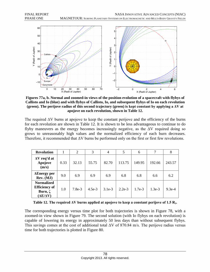
FINAL REPORT NASA INNOVATIVE ADVANCED CONCEPTS (NIAC) PHASE ONE MAGNETOUR: SURFING PLANETARY SYSTEMS ON ELECTROMAGNETIC AND MULTI-BODY GRAVITY FIELDS
Figures 77a, b. Normal and zoomed-in views of the position evolution of a spacecraft with flybys of Callisto and Io (blue) and with flybys of Callisto, Io, and subsequent flybys of Io on each revolution (green). The perijove radius of this second trajectory (green) is kept constant by applying a ΔV at
apojove on each revolution, shown in Table 12.
The required ΔV burns at apojove to keep the constant perijove and the efficiency of the burns for each revolution are shown in Table 12. It is shown to be less advantageous to continue to do flyby maneuvers as the energy becomes increasingly negative, as the ΔV required doing so grows to unreasonably high values and the normalized efficiency of each burn decreases. Therefore, it recommended that ΔV burns be performed only on the first or first few revolutions.
Revolution 1 2 3 4 5 6 7 8
ΔV req’d at Apojove
(m/s) 0.33 32.13 55.75 82.70 113.75 149.95 192.66 243.57
ΔEnergy per Rev. (MJ) 9.0 6.9 6.9 6.9 6.8 6.8 6.6 6.2
Normalized Efficiency of
Burn, ζ 1.0 7.8e-3 4.5e-3 3.1e-3 2.2e-3 1.7e-3 1.3e-3 9.3e-4
(ΔE/ΔV)
Table 12. The required ΔV burns applied at apojove to keep a constant perijove of 1.5 RJ.
The corresponding energy versus time plot for both trajectories is shown in Figure 78, with a zoomed-in view shown in Figure 79. The second solution (with Io flybys on each revolution) is capable of lowering its energy in approximately 50 less days than without subsequent flybys. This savings comes at the cost of additional total ΔV of 870.84 m/s. The perijove radius versus time for both trajectories is plotted in Figure 80.
78 Copyright 2013. All rights reserved.
Callisto
Ganymede
EuropaIo
Io
0 10 20 30 40 50 60 70
−10
0
10
20
30
40
50
60
X (Radii of Jupiter)
Y (R
adii
of J
upite
r)
−2 0 2 4 6
−1
−2
0
1
2
3
4
5
X (Radii of Jupiter)
Y (R
adii
of J
upite
r)
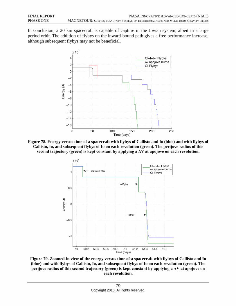
FINAL REPORT NASA INNOVATIVE ADVANCED CONCEPTS (NIAC) PHASE ONE MAGNETOUR: SURFING PLANETARY SYSTEMS ON ELECTROMAGNETIC AND MULTI-BODY GRAVITY FIELDS
In conclusion, a 20 km spacecraft is capable of capture in the Jovian system, albeit in a large period orbit. The addition of flybys on the inward-bound path gives a free performance increase, although subsequent flybys may not be beneficial.
Figure 78. Energy versus time of a spacecraft with flybys of Callisto and Io (blue) and with flybys of Callisto, Io, and subsequent flybys of Io on each revolution (green). The perijove radius of this
second trajectory (green) is kept constant by applying a ΔV at apojove on each revolution.
Figure 79. Zoomed-in view of the energy versus time of a spacecraft with flybys of Callisto and Io (blue) and with flybys of Callisto, Io, and subsequent flybys of Io on each revolution (green). The perijove radius of this second trajectory (green) is kept constant by applying a ΔV at apojove on
each revolution.
79 Copyright 2013. All rights reserved.
−10
−12
−14
−16
0 50 100 150 200 250
−2
−4
−6
−8
0
2
4x 10⁷
Ener
gy (J
)
Time (days)
CI−I−I−I Flybysw/ apojove burnsCI Flybys
50 50.2 50.4 50.6 50.8 51 51.2 51.4 51.6 51.8
−1
−0.5
0
0.5
1
x 107
Ener
gy (J
)
Time (days)
CI−I−I−I Flybysw/ apojove burnsCI FlybysCallisto Flyby
Io Flyby
Tether
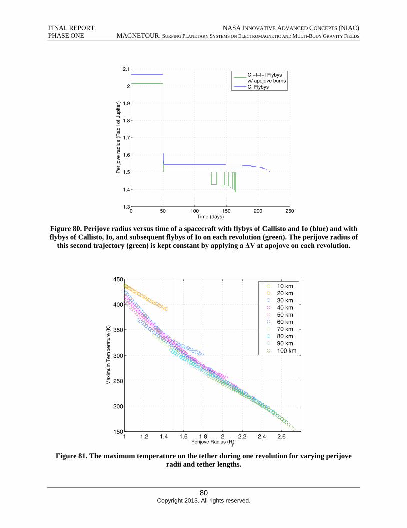
FINAL REPORT NASA INNOVATIVE ADVANCED CONCEPTS (NIAC) PHASE ONE MAGNETOUR: SURFING PLANETARY SYSTEMS ON ELECTROMAGNETIC AND MULTI-BODY GRAVITY FIELDS
Figure 80. Perijove radius versus time of a spacecraft with flybys of Callisto and Io (blue) and with flybys of Callisto, Io, and subsequent flybys of Io on each revolution (green). The perijove radius of
this second trajectory (green) is kept constant by applying a ΔV at apojove on each revolution.
Figure 81. The maximum temperature on the tether during one revolution for varying perijove radii and tether lengths.
80 Copyright 2013. All rights reserved.
0 50 100 150 200 250
1.4
1.5
1.6
1.7
1.8
1.9
2
2.1
Time (days)
Perij
ove
radi
us (R
adii
of J
upite
r)
1.3
CI−I−I−I Flybysw/ apojove burnsCI Flybys
1 1.2 1.4 1.6 1.8 2 2.2 2.4 2.6
200
250
300
350
400
450
Perijove Radius (Rj)
Max
imum
Tem
pera
ture
(K)
150
10 km20 km30 km40 km50 km60 km70 km80 km90 km100 km
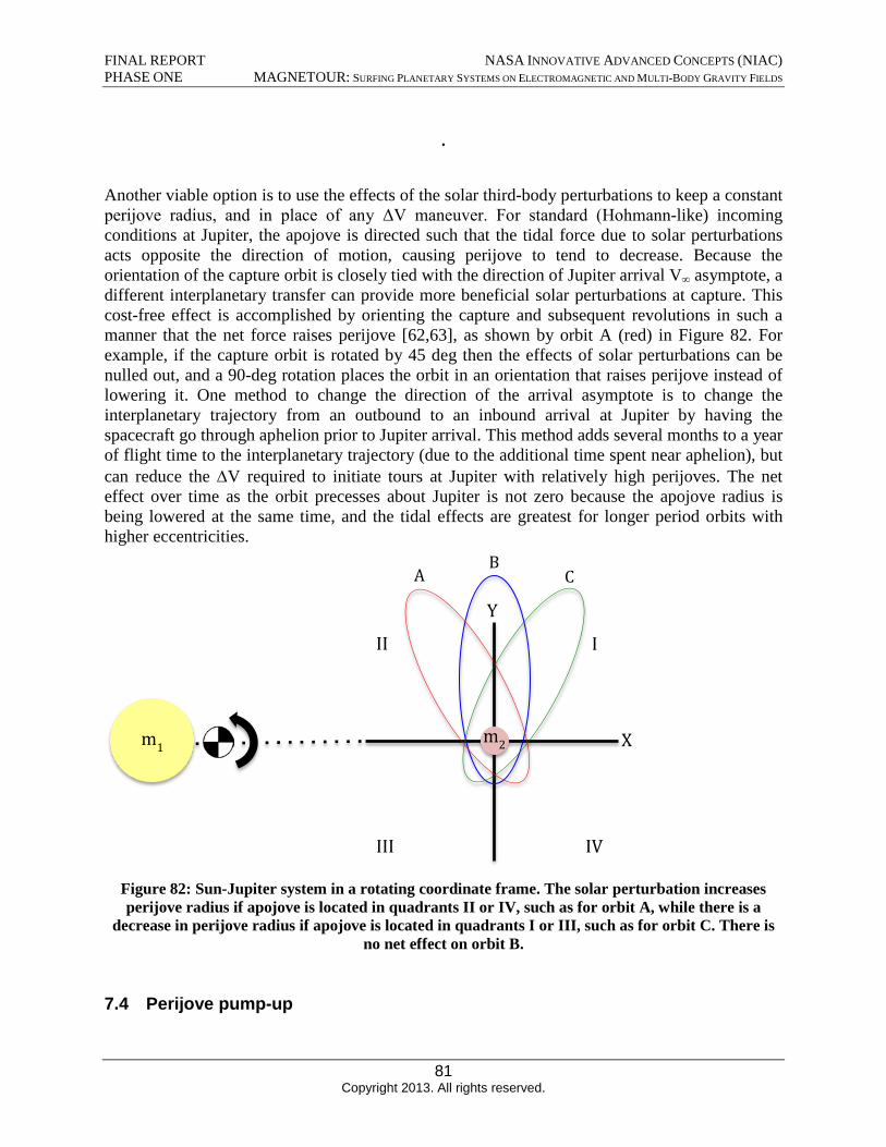
FINAL REPORT NASA INNOVATIVE ADVANCED CONCEPTS (NIAC) PHASE ONE MAGNETOUR: SURFING PLANETARY SYSTEMS ON ELECTROMAGNETIC AND MULTI-BODY GRAVITY FIELDS
.
Another viable option is to use the effects of the solar third-body perturbations to keep a constant perijove radius, and in place of any ΔV maneuver. For standard (Hohmann-like) incoming conditions at Jupiter, the apojove is directed such that the tidal force due to solar perturbations acts opposite the direction of motion, causing perijove to tend to decrease. Because the orientation of the capture orbit is closely tied with the direction of Jupiter arrival V∞ asymptote, a different interplanetary transfer can provide more beneficial solar perturbations at capture. This cost-free effect is accomplished by orienting the capture and subsequent revolutions in such a manner that the net force raises perijove [62,63], as shown by orbit A (red) in Figure 82. For example, if the capture orbit is rotated by 45 deg then the effects of solar perturbations can be nulled out, and a 90-deg rotation places the orbit in an orientation that raises perijove instead of lowering it. One method to change the direction of the arrival asymptote is to change the interplanetary trajectory from an outbound to an inbound arrival at Jupiter by having the spacecraft go through aphelion prior to Jupiter arrival. This method adds several months to a year of flight time to the interplanetary trajectory (due to the additional time spent near aphelion), but can reduce the ΔV required to initiate tours at Jupiter with relatively high perijoves. The net effect over time as the orbit precesses about Jupiter is not zero because the apojove radius is being lowered at the same time, and the tidal effects are greatest for longer period orbits with higher eccentricities.
Figure 82: Sun-Jupiter system in a rotating coordinate frame. The solar perturbation increases perijove radius if apojove is located in quadrants II or IV, such as for orbit A, while there is a
decrease in perijove radius if apojove is located in quadrants I or III, such as for orbit C. There is no net effect on orbit B.
7.4 Perijove pump-up
Y
Xm1
III
m2
A B
C
III IV
81 Copyright 2013. All rights reserved.
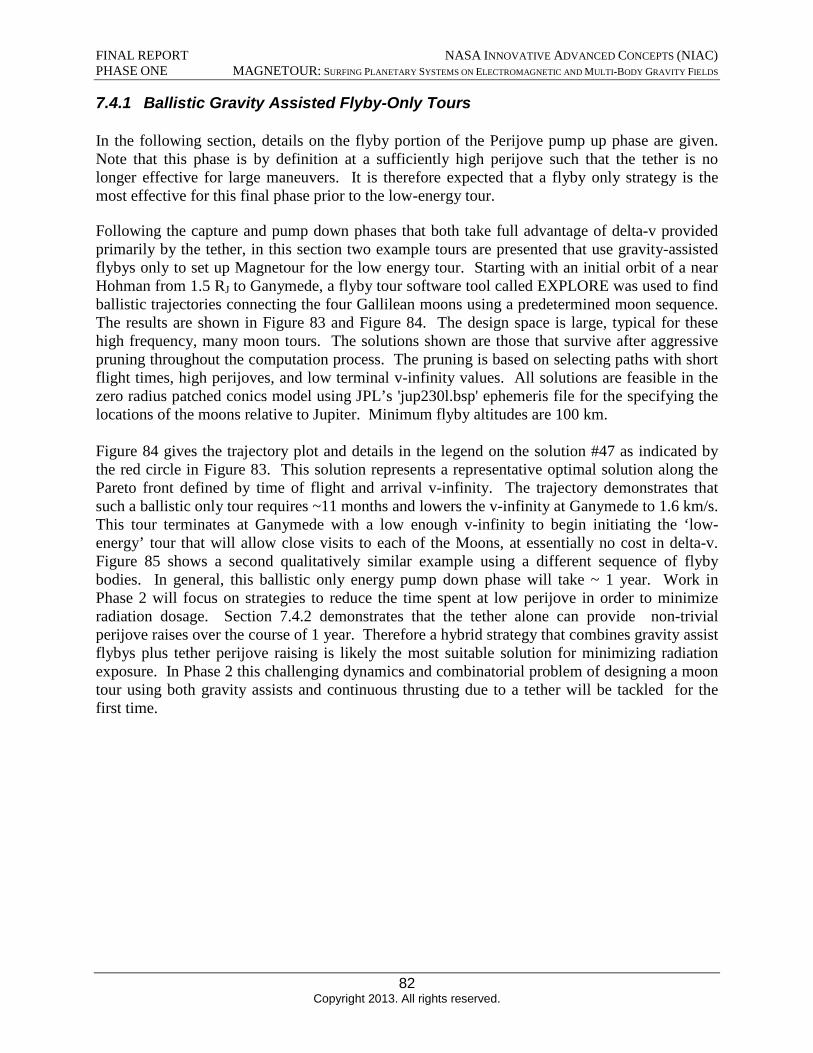
FINAL REPORT NASA INNOVATIVE ADVANCED CONCEPTS (NIAC) PHASE ONE MAGNETOUR: SURFING PLANETARY SYSTEMS ON ELECTROMAGNETIC AND MULTI-BODY GRAVITY FIELDS
7.4.1 Ballistic Gravity Assisted Flyby-Only Tours
In the following section, details on the flyby portion of the Perijove pump up phase are given. Note that this phase is by definition at a sufficiently high perijove such that the tether is no longer effective for large maneuvers. It is therefore expected that a flyby only strategy is the most effective for this final phase prior to the low-energy tour.
Following the capture and pump down phases that both take full advantage of delta-v provided primarily by the tether, in this section two example tours are presented that use gravity-assisted flybys only to set up Magnetour for the low energy tour. Starting with an initial orbit of a near Hohman from 1.5 RJ to Ganymede, a flyby tour software tool called EXPLORE was used to find ballistic trajectories connecting the four Gallilean moons using a predetermined moon sequence. The results are shown in Figure 83 and Figure 84. The design space is large, typical for these high frequency, many moon tours. The solutions shown are those that survive after aggressive pruning throughout the computation process. The pruning is based on selecting paths with short flight times, high perijoves, and low terminal v-infinity values. All solutions are feasible in the zero radius patched conics model using JPL’s 'jup230l.bsp' ephemeris file for the specifying the locations of the moons relative to Jupiter. Minimum flyby altitudes are 100 km.
Figure 84 gives the trajectory plot and details in the legend on the solution #47 as indicated by the red circle in Figure 83. This solution represents a representative optimal solution along the Pareto front defined by time of flight and arrival v-infinity. The trajectory demonstrates that such a ballistic only tour requires ~11 months and lowers the v-infinity at Ganymede to 1.6 km/s. This tour terminates at Ganymede with a low enough v-infinity to begin initiating the ‘lowenergy’ tour that will allow close visits to each of the Moons, at essentially no cost in delta-v. Figure 85 shows a second qualitatively similar example using a different sequence of flyby bodies. In general, this ballistic only energy pump down phase will take ~ 1 year. Work in Phase 2 will focus on strategies to reduce the time spent at low perijove in order to minimize radiation dosage. Section 7.4.2 demonstrates that the tether alone can provide non-trivial perijove raises over the course of 1 year. Therefore a hybrid strategy that combines gravity assist flybys plus tether perijove raising is likely the most suitable solution for minimizing radiation exposure. In Phase 2 this challenging dynamics and combinatorial problem of designing a moon tour using both gravity assists and continuous thrusting due to a tether will be tackled for the first time.
82 Copyright 2013. All rights reserved.
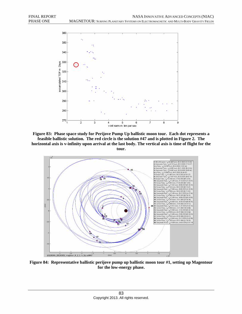
FINAL REPORT NASA INNOVATIVE ADVANCED CONCEPTS (NIAC) PHASE ONE MAGNETOUR: SURFING PLANETARY SYSTEMS ON ELECTROMAGNETIC AND MULTI-BODY GRAVITY FIELDS
Figure 83: Phase space study for Perijove Pump Up ballistic moon tour. Each dot represents a feasible ballistic solution. The red circle is the solution #47 and is plotted in Figure 2. The
horizontal axis is v-infinity upon arrival at the last body. The vertical axis is time of flight for the tour.
Figure 84: Representative ballistic perijove pump up ballistic moon tour #1, setting up Magentour for the low-energy phase.
83 Copyright 2013. All rights reserved.
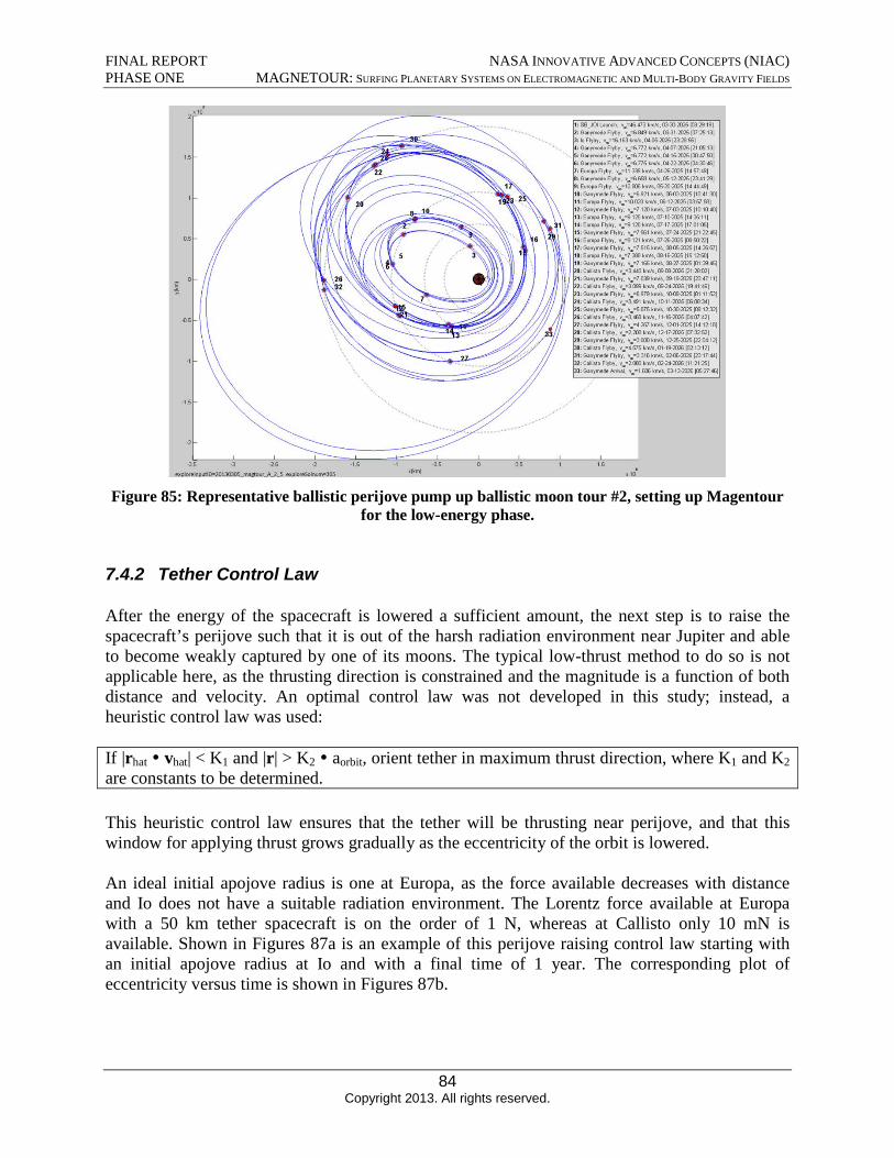
|rhat • vhat| < K1 and |r| > K2 • aorbit,
FINAL REPORT NASA INNOVATIVE ADVANCED CONCEPTS (NIAC) PHASE ONE MAGNETOUR: SURFING PLANETARY SYSTEMS ON ELECTROMAGNETIC AND MULTI-BODY GRAVITY FIELDS
Figure 85: Representative ballistic perijove pump up ballistic moon tour #2, setting up Magentour for the low-energy phase.
7.4.2 Tether Control Law
After the energy of the spacecraft is lowered a sufficient amount, the next step is to raise the spacecraft’s perijove such that it is out of the harsh radiation environment near Jupiter and able to become weakly captured by one of its moons. The typical low-thrust method to do so is not applicable here, as the thrusting direction is constrained and the magnitude is a function of both distance and velocity. An optimal control law was not developed in this study; instead, a heuristic control law was used:
If orient tether in maximum thrust direction, where K1 and K2are constants to be determined.
This heuristic control law ensures that the tether will be thrusting near perijove, and that this window for applying thrust grows gradually as the eccentricity of the orbit is lowered.
An ideal initial apojove radius is one at Europa, as the force available decreases with distance and Io does not have a suitable radiation environment. The Lorentz force available at Europa with a 50 km tether spacecraft is on the order of 1 N, whereas at Callisto only 10 mN is available. Shown in Figures 87a is an example of this perijove raising control law starting with an initial apojove radius at Io and with a final time of 1 year. The corresponding plot of eccentricity versus time is shown in Figures 87b.
84 Copyright 2013. All rights reserved.
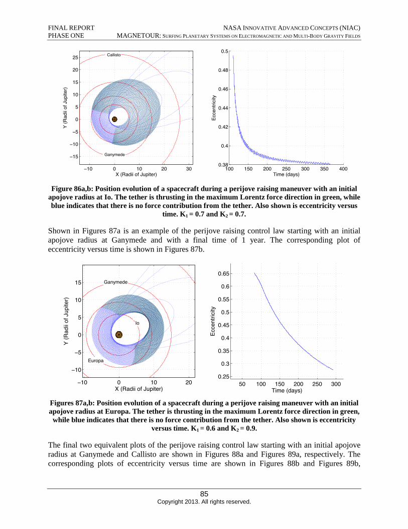
FINAL REPORT NASA INNOVATIVE ADVANCED CONCEPTS (NIAC) PHASE ONE MAGNETOUR: SURFING PLANETARY SYSTEMS ON ELECTROMAGNETIC AND MULTI-BODY GRAVITY FIELDS
Figure 86a,b: Position evolution of a spacecraft during a perijove raising maneuver with an initial apojove radius at Io. The tether is thrusting in the maximum Lorentz force direction in green, while blue indicates that there is no force contribution from the tether. Also shown is eccentricity versus
time. K1 = 0.7 and K2 = 0.7.
Shown in Figures 87a is an example of the perijove raising control law starting with an initial apojove radius at Ganymede and with a final time of 1 year. The corresponding plot of eccentricity versus time is shown in Figures 87b.
Figures 87a,b: Position evolution of a spacecraft during a perijove raising maneuver with an initial apojove radius at Europa. The tether is thrusting in the maximum Lorentz force direction in green,
while blue indicates that there is no force contribution from the tether. Also shown is eccentricity versus time. K1 = 0.6 and K2 = 0.9.
The final two equivalent plots of the perijove raising control law starting with an initial apojove radius at Ganymede and Callisto are shown in Figures 88a and Figures 89a, respectively. The corresponding plots of eccentricity versus time are shown in Figures 88b and Figures 89b,
85 Copyright 2013. All rights reserved.
Ganymede
Callisto
−10 0 10 20 30
−10
−15
−5
0
5
10
15
20
25
X (Radii of Jupiter)
Y (R
adii
of J
upite
r)
100 150 200 250 300 350 4000.38
0.4
0.42
0.44
0.46
0.48
0.5
Time (days)
Ecce
ntric
ity
Ganymede
Io
−10
−10 20
−5
0
5
10
15
0 10X (Radii of Jupiter)
Y (R
adii
of J
upite
r)
50 100 150 200 250 3000.25
0.3
0.35
0.4
0.45
0.5
0.55
0.6
0.65
Time (days)
Ecce
ntric
ity
Europa
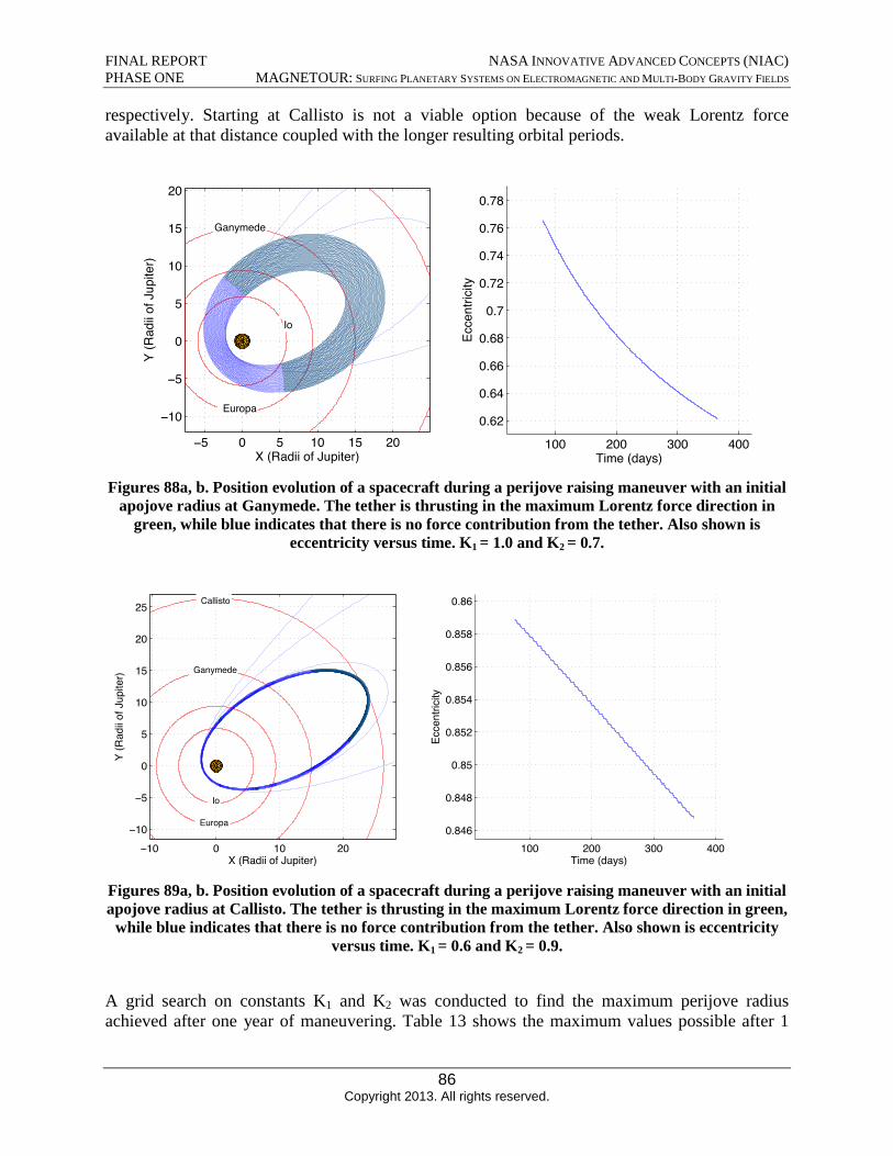
FINAL REPORT NASA INNOVATIVE ADVANCED CONCEPTS (NIAC) PHASE ONE MAGNETOUR: SURFING PLANETARY SYSTEMS ON ELECTROMAGNETIC AND MULTI-BODY GRAVITY FIELDS
respectively. Starting at Callisto is not a viable option because of the weak Lorentz force available at that distance coupled with the longer resulting orbital periods.
Figures 88a, b. Position evolution of a spacecraft during a perijove raising maneuver with an initial apojove radius at Ganymede. The tether is thrusting in the maximum Lorentz force direction in
green, while blue indicates that there is no force contribution from the tether. Also shown is eccentricity versus time. K1 = 1.0 and K2 = 0.7.
Figures 89a, b. Position evolution of a spacecraft during a perijove raising maneuver with an initial apojove radius at Callisto. The tether is thrusting in the maximum Lorentz force direction in green,
while blue indicates that there is no force contribution from the tether. Also shown is eccentricity versus time. K1 = 0.6 and K2 = 0.9.
A grid search on constants K1 and K2 was conducted to find the maximum perijove radius achieved after one year of maneuvering. Table 13 shows the maximum values possible after 1
86 Copyright 2013. All rights reserved.
−5 0 20
−10
−5
0
5
10
15
20
5 10 15X (Radii of Jupiter)
Y (R
adii
of J
upite
r)
100 200 300 400
0.62
0.64
0.66
0.68
0.7
0.72
0.74
0.76
0.78
Time (days)Ec
cent
ricity
Europa
Io
Ganymede
−10−10 0 20
−5
0
5
10
15
20
25
10X (Radii of Jupiter)
Y (R
adii
of J
upite
r)
100 200 300 4000.846
0.848
0.85
0.852
0.854
0.856
0.858
0.86
Time (days)
Ecce
ntric
ity
Callisto
Ganymede
Europa
Io
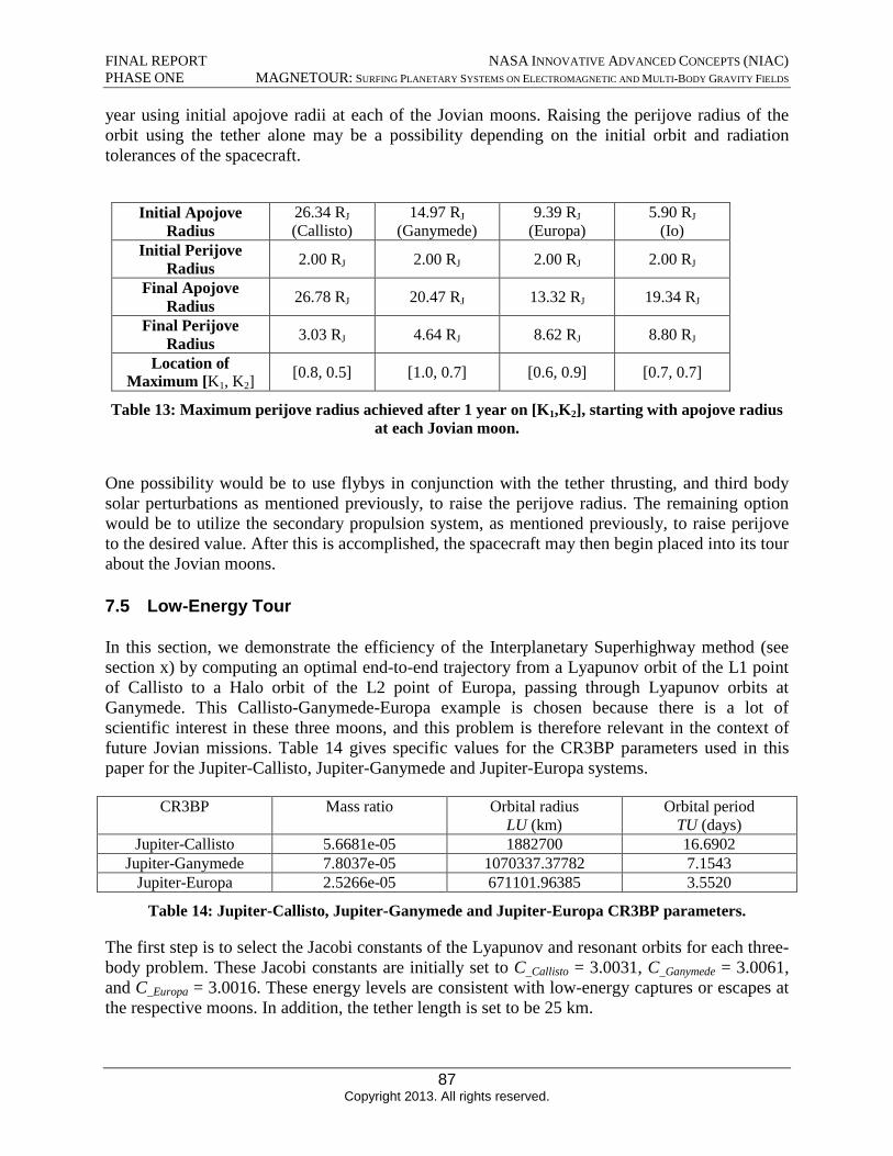
FINAL REPORT NASA INNOVATIVE ADVANCED CONCEPTS (NIAC) PHASE ONE MAGNETOUR: SURFING PLANETARY SYSTEMS ON ELECTROMAGNETIC AND MULTI-BODY GRAVITY FIELDS
year using initial apojove radii at each of the Jovian moons. Raising the perijove radius of the orbit using the tether alone may be a possibility depending on the initial orbit and radiation tolerances of the spacecraft.
Initial Apojove Radius
26.34 RJ (Callisto)
14.97 RJ (Ganymede)
9.39 RJ (Europa)
5.90 RJ (Io)
Initial Perijove Radius 2.00 RJ 2.00 RJ 2.00 RJ 2.00 RJ
Final Apojove Radius 26.78 RJ 20.47 RJ 13.32 RJ 19.34 RJ
Final Perijove Radius 3.03 RJ 4.64 RJ 8.62 RJ 8.80 RJ
Location of Maximum [K1, K2]
[0.8, 0.5] [1.0, 0.7] [0.6, 0.9] [0.7, 0.7]
Table 13: Maximum perijove radius achieved after 1 year on [K1,K2], starting with apojove radius at each Jovian moon.
One possibility would be to use flybys in conjunction with the tether thrusting, and third body solar perturbations as mentioned previously, to raise the perijove radius. The remaining option would be to utilize the secondary propulsion system, as mentioned previously, to raise perijove to the desired value. After this is accomplished, the spacecraft may then begin placed into its tour about the Jovian moons.
7.5 Low-Energy Tour
In this section, we demonstrate the efficiency of the Interplanetary Superhighway method (see section x) by computing an optimal end-to-end trajectory from a Lyapunov orbit of the L1 point of Callisto to a Halo orbit of the L2 point of Europa, passing through Lyapunov orbits at Ganymede. This Callisto-Ganymede-Europa example is chosen because there is a lot of scientific interest in these three moons, and this problem is therefore relevant in the context of future Jovian missions. Table 14 gives specific values for the CR3BP parameters used in this paper for the Jupiter-Callisto, Jupiter-Ganymede and Jupiter-Europa systems.
CR3BP Mass ratio Orbital radius LU (km)
Orbital period TU (days)
Jupiter-Callisto 5.6681e-05 1882700 16.6902 Jupiter-Ganymede 7.8037e-05 1070337.37782 7.1543
Jupiter-Europa 2.5266e-05 671101.96385 3.5520
Table 14: Jupiter-Callisto, Jupiter-Ganymede and Jupiter-Europa CR3BP parameters.
The first step is to select the Jacobi constants of the Lyapunov and resonant orbits for each three-body problem. These Jacobi constants are initially set to C_Callisto = 3.0031, C_Ganymede = 3.0061, and C_Europa = 3.0016. These energy levels are consistent with low-energy captures or escapes at the respective moons. In addition, the tether length is set to be 25 km.
87 Copyright 2013. All rights reserved.
FINAL REPORT NASA INNOVATIVE ADVANCED CONCEPTS (NIAC) PHASE ONE MAGNETOUR: SURFING PLANETARY SYSTEMS ON ELECTROMAGNETIC AND MULTI-BODY GRAVITY FIELDS
The next step is to generate a good initial guess of the solution. On the Callisto dominant phase, the trajectory begins on a L1 Lyapunov orbit at Callisto and proceeds to the near-Hohmann orbit with the following sequence: L1 Lyapunov ➔ Lyapunov Unstable Manifold ➔ 5:6 ➔ 4:5 ➔ 7:9 ➔ 3:4 ➔ 8:11 ➔ 5:7 ➔ 7:10. The initial resonance 5:6 is chosen because it is the lowestresonance that can be reached by simply ‘falling off’ the Lyapunov orbit. The choice of the otherresonances is the result of several trial-and-error optimizations to find a good resonant path.Similarly, the resonant path of the Ganymede exterior portion is (in backward time): L2Lyapunov ➔ Lyapunov Stable Manifold ➔ 4:3 ➔ 7:5 ➔ 3:2. A quasi-ballistic heteroclinicconnection (see section 5.2.2) is then computed for the transfer from a L2 Lyapunov orbit to a L1Lyapunov orbit at Ganymede. The resonant path of the Ganymede interior portion is next: L1Lyapunov ➔ Lyapunov Unstable Manifold ➔ 4:5 ➔ 7:9 ➔ 3:4 ➔ 8:11. Finally, the resonantpath of the Europa exterior portion is (in backward time): L2 Lyapunov ➔ Lyapunov StableManifold ➔ 5:4 ➔ 9:7 ➔ 4:3 ➔ 11:8 ➔ 7:5. For this overall transfer, there are therefore 20moon flybys in total: 7 Callisto flybys, 8 Ganymede flybys, and 4 Europa flybys.
The optimization of this problem is performed using the OPTIFOR tool [53] with the Intel Fortran compiler. All constraints are enforced with a normalized tolerance of 10-8, which corresponds to position and velocity discontinuities of around 10 m and 0.1 mm/s respectively. Targeting such a high tolerance is facilitated by the robust multi-shooting implementation.
The resulting optimized solution requires a total delta-v of 5 m/s only, and the total flight time is 1120 days, which is well within conceivable mission constraints. The small maneuvers are performed by the tether. Our objective to find a propellantless transfer is therefore achieved. We emphasize that the trajectory does include phasing and several fully integrated flybys of Callisto, Ganymede and Europa. The corresponding entire trajectory is shown in the inertial frame and in the rotating frames of the patched CR3BP model in Figure 90 - Figure 94. Time history of theorbital radius of the trajectory is given in Figure 95. We can see that the orbital radius is decreasing sequentially, as expected. First, the trajectory gets its perijove reduced with flybys of Callisto. Then, the spacecraft passes naturally to the control of Ganymede and accordingly reduces its apojove. Then the spacecraft travels to the interior resonances of Ganymede and gets its perijove reduced. Finally, the trajectory gets its apojove reduced with flybys of Europa. Example of the tether thrust profile is given in Figure 96 for the interior Ganymede-dominated portion. The required Lorentz force always stays below the maximum Lorentz force achievable by the tether.
Further insight of the dynamics is seen when plotting the spacecraft trajectory on the T-P graph, a new graphical tool introduced by Campagnola and Russell [64] (see Figure 97). On the T-P graph, level sets of constant Tisserand parameter are plotted in ($r_a$, $r_p$) space where the Tisserand parameter is almost equivalent to the Jacobi constant of the PR3BP. During the resonance hopping transfer, the spacecraft jumps between resonances (represented by big dots) along the level sets of Tisserand curves. Overall, the transfer orbit scarcely deviating from curves of constant Tisserand parameter, due to the small tether maneuvers.
88 Copyright 2013. All rights reserved.
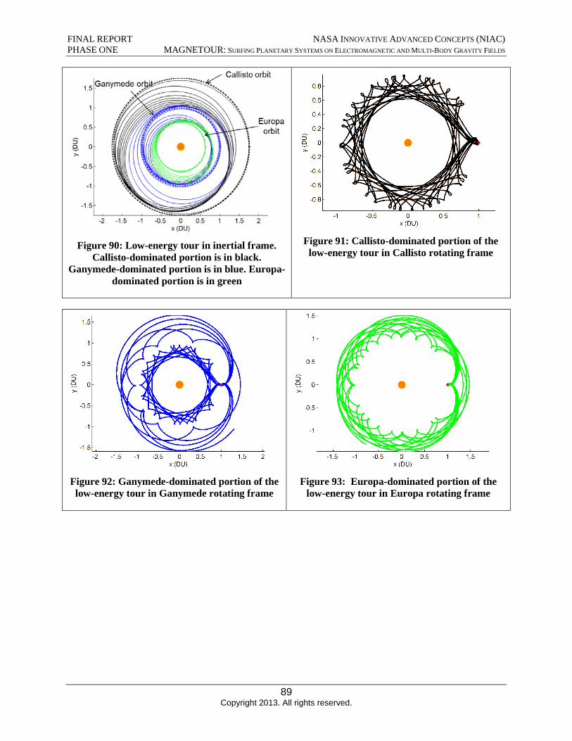
FINAL REPORT NASA INNOVATIVE ADVANCED CONCEPTS (NIAC) PHASE ONE MAGNETOUR: SURFING PLANETARY SYSTEMS ON ELECTROMAGNETIC AND MULTI-BODY GRAVITY FIELDS
Figure 90: Low-energy tour in inertial frame. Callisto-dominated portion is in black.
Ganymede-dominated portion is in blue. Europa-dominated portion is in green
Figure 91: Callisto-dominated portion of the low-energy tour in Callisto rotating frame
Figure 92: Ganymede-dominated portion of the low-energy tour in Ganymede rotating frame
Figure 93: Europa-dominated portion of the low-energy tour in Europa rotating frame
89 Copyright 2013. All rights reserved.
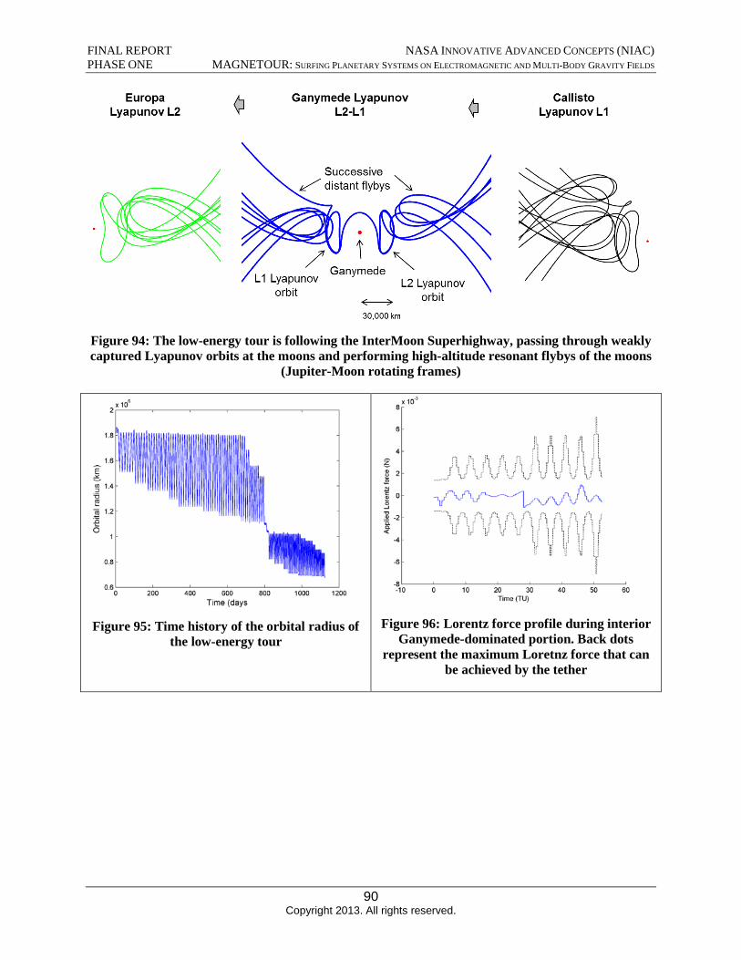
FINAL REPORT NASA INNOVATIVE ADVANCED CONCEPTS (NIAC) PHASE ONE MAGNETOUR: SURFING PLANETARY SYSTEMS ON ELECTROMAGNETIC AND MULTI-BODY GRAVITY FIELDS
Figure 94: The low-energy tour is following the InterMoon Superhighway, passing through weakly captured Lyapunov orbits at the moons and performing high-altitude resonant flybys of the moons
(Jupiter-Moon rotating frames)
Figure 95: Time history of the orbital radius of the low-energy tour
Figure 96: Lorentz force profile during interior Ganymede-dominated portion. Back dots
represent the maximum Loretnz force that can be achieved by the tether
90 Copyright 2013. All rights reserved.
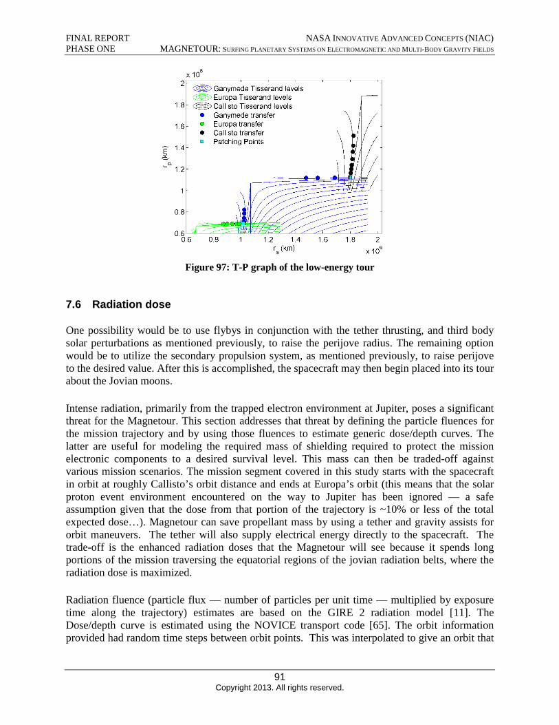
FINAL REPORT NASA INNOVATIVE ADVANCED CONCEPTS (NIAC) PHASE ONE MAGNETOUR: SURFING PLANETARY SYSTEMS ON ELECTROMAGNETIC AND MULTI-BODY GRAVITY FIELDS
Figure 97: T-P graph of the low-energy tour
7.6 Radiation dose
One possibility would be to use flybys in conjunction with the tether thrusting, and third body solar perturbations as mentioned previously, to raise the perijove radius. The remaining option would be to utilize the secondary propulsion system, as mentioned previously, to raise perijove to the desired value. After this is accomplished, the spacecraft may then begin placed into its tour about the Jovian moons.
Intense radiation, primarily from the trapped electron environment at Jupiter, poses a significant threat for the Magnetour. This section addresses that threat by defining the particle fluences for the mission trajectory and by using those fluences to estimate generic dose/depth curves. The latter are useful for modeling the required mass of shielding required to protect the mission electronic components to a desired survival level. This mass can then be traded-off against various mission scenarios. The mission segment covered in this study starts with the spacecraft in orbit at roughly Callisto’s orbit distance and ends at Europa’s orbit (this means that the solar proton event environment encountered on the way to Jupiter has been ignored — a safe assumption given that the dose from that portion of the trajectory is ~10% or less of the total expected dose…). Magnetour can save propellant mass by using a tether and gravity assists for orbit maneuvers. The tether will also supply electrical energy directly to the spacecraft. The trade-off is the enhanced radiation doses that the Magnetour will see because it spends long portions of the mission traversing the equatorial regions of the jovian radiation belts, where the radiation dose is maximized.
Radiation fluence (particle flux — number of particles per unit time — multiplied by exposure time along the trajectory) estimates are based on the GIRE 2 radiation model [11]. The Dose/depth curve is estimated using the NOVICE transport code [65]. The orbit information provided had random time steps between orbit points. This was interpolated to give an orbit that
91 Copyright 2013. All rights reserved.
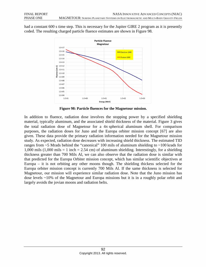
Particle Fluence Magnetour
1.E+17
1.E+16
1.E+15
1.E+14
1.E+13
1.E+12
1.E+11
1.E+10
1.E+09
1.E+08
1.E+07
1.E+06
1.E+05
1.E+04 1.E-01 1.E+00
Electron GIRE
Proton GIRE Fl
uenc
e (c
m-1
)
1.E+01 1.E+02 1.E+03
Energy (MeV)
FINAL REPORT NASA INNOVATIVE ADVANCED CONCEPTS (NIAC) PHASE ONE MAGNETOUR: SURFING PLANETARY SYSTEMS ON ELECTROMAGNETIC AND MULTI-BODY GRAVITY FIELDS
had a constant 600 s time step. This is necessary for the Jupiter GIRE 2 program as it is presently coded. The resulting charged particle fluence estimates are shown in Figure 98.
Figure 98: Particle fluences for the Magnetour mission.
In addition to fluence, radiation dose involves the stopping power by a specified shielding material, typically aluminum, and the associated shield thickness of the material. Figure 3 gives the total radiation dose of Magnetour for a 4π spherical aluminum shell. For comparison purposes, the radiation doses for Juno and the Europa orbiter mission concept [67] are also given. These data provide the primary radiation information needed for the Magnetour mission study. As expected, radiation dose decreases with increasing shield thickness. The estimated TID ranges from ~5 Mrads behind the “canonical” 100 mils of aluminum shielding to ~100 krads for 1,000 mils (1,000 mils = 1 inch = 2.54 cm) of aluminum shielding. Interestingly, for a shielding thickness greater than 700 Mils Al, we can also observe that the radiation dose is similar with that predicted for the Europa Orbiter mission concept, which has similar scientific objectives at Europa – it is not orbiting any other moons though. The shielding thickess selected for the Europa orbiter mission concept is currently 700 Mils Al. If the same thickness is selected for Magnetour, our mission will experience similar radiation dose. Note that the Juno mission has dose levels ~10% of the Magnetour and Europa missions but it is in a roughly polar orbit and largely avoids the jovian moons and radiation belts.
92 Copyright 2013. All rights reserved.
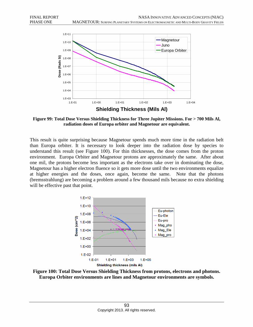
Dos
e (R
ads
Si)
1.E+11
1.E+10
1.E+09
1.E+08
1.E+07
1.E+06
1.E+05
1.E+04
1.E+03
Magnetour Juno Europa Orbiter
1.E-01 1.E+00 1.E+01 1.E+02 1.E+03 1.E+04
Shielding Thickness (Mils Al)
FINAL REPORT NASA INNOVATIVE ADVANCED CONCEPTS (NIAC) PHASE ONE MAGNETOUR: SURFING PLANETARY SYSTEMS ON ELECTROMAGNETIC AND MULTI-BODY GRAVITY FIELDS
Figure 99: Total Dose Versus Shielding Thickness for Three Jupiter Missions. For > 700 Mils Al, radiation doses of Europa orbiter and Magnetour are equivalent.
This result is quite surprising because Magnetour spends much more time in the radiation belt than Europa orbiter. It is necessary to look deeper into the radiation dose by species to understand this result (see Figure 100). For thin thicknesses, the dose comes from the proton environment. Europa Orbiter and Magnetour protons are approximately the same. After about one mil, the protons become less important as the electrons take over in dominating the dose, Magnetour has a higher electron fluence so it gets more dose until the two environments equalize at higher energies and the doses, once again, become the same. Note that the photons (bremsstrahlung) are becoming a problem around a few thousand mils because no extra shielding will be effective past that point.
Figure 100: Total Dose Versus Shielding Thickness from protons, electrons and photons. Europa Orbiter environments are lines and Magnetour environments are symbols.
93 Copyright 2013. All rights reserved.
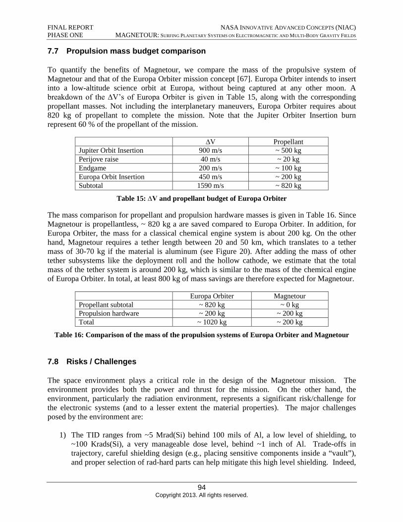
FINAL REPORT NASA INNOVATIVE ADVANCED CONCEPTS (NIAC) PHASE ONE MAGNETOUR: SURFING PLANETARY SYSTEMS ON ELECTROMAGNETIC AND MULTI-BODY GRAVITY FIELDS
7.7 Propulsion mass budget comparison
To quantify the benefits of Magnetour, we compare the mass of the propulsive system of Magnetour and that of the Europa Orbiter mission concept [67]. Europa Orbiter intends to insert into a low-altitude science orbit at Europa, without being captured at any other moon. A breakdown of the ΔV’s of Europa Orbiter is given in Table 15, along with the corresponding propellant masses. Not including the interplanetary maneuvers, Europa Orbiter requires about 820 kg of propellant to complete the mission. Note that the Jupiter Orbiter Insertion burn represent 60 % of the propellant of the mission.
ΔV Propellant Jupiter Orbit Insertion 900 m/s ~ 500 kg Perijove raise 40 m/s ~ 20 kg Endgame 200 m/s ~ 100 kg Europa Orbit Insertion 450 m/s ~ 200 kg Subtotal 1590 m/s ~ 820 kg
Table 15: ΔV and propellant budget of Europa Orbiter
The mass comparison for propellant and propulsion hardware masses is given in Table 16. Since Magnetour is propellantless, ~ 820 kg a are saved compared to Europa Orbiter. In addition, for Europa Orbiter, the mass for a classical chemical engine system is about 200 kg. On the other hand, Magnetour requires a tether length between 20 and 50 km, which translates to a tether mass of 30-70 kg if the material is aluminum (see Figure 20). After adding the mass of other tether subsystems like the deployment roll and the hollow cathode, we estimate that the total mass of the tether system is around 200 kg, which is similar to the mass of the chemical engine of Europa Orbiter. In total, at least 800 kg of mass savings are therefore expected for Magnetour.
Europa Orbiter Magnetour Propellant subtotal ~ 820 kg ~ 0 kg Propulsion hardware ~ 200 kg ~ 200 kg Total ~ 1020 kg ~ 200 kg
Table 16: Comparison of the mass of the propulsion systems of Europa Orbiter and Magnetour
7.8 Risks / Challenges
The space environment plays a critical role in the design of the Magnetour mission. The environment provides both the power and thrust for the mission. On the other hand, the environment, particularly the radiation environment, represents a significant risk/challenge for the electronic systems (and to a lesser extent the material properties). The major challenges posed by the environment are:
1) The TID ranges from ~5 Mrad(Si) behind 100 mils of Al, a low level of shielding, to~100 Krads(Si), a very manageable dose level, behind ~1 inch of Al. Trade-offs intrajectory, careful shielding design (e.g., placing sensitive components inside a “vault”),and proper selection of rad-hard parts can help mitigate this high level shielding. Indeed,
94 Copyright 2013. All rights reserved.
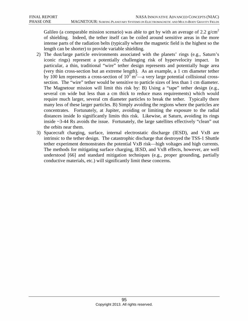
FINAL REPORT NASA INNOVATIVE ADVANCED CONCEPTS (NIAC) PHASE ONE MAGNETOUR: SURFING PLANETARY SYSTEMS ON ELECTROMAGNETIC AND MULTI-BODY GRAVITY FIELDS
Galileo (a comparable mission scenario) was able to get by with an average of 2.2 g/cm2
of shielding. Indeed, the tether itself can be coiled around sensitive areas in the more intense parts of the radiation belts (typically where the magnetic field is the highest so the length can be shorter) to provide variable shielding.
2) The dust/large particle environments associated with the planets’ rings (e.g., Saturn’siconic rings) represent a potentially challenging risk of hypervelocity impact. Inparticular, a thin, traditional “wire” tether design represents and potentially huge area(very thin cross-section but an extreme length). As an example, a 1 cm diameter tetherby 100 km represents a cross-section of 103 m2—a very large potential collisional cross-section. The “wire” tether would be sensitive to particle sizes of less than 1 cm diameter.The Magnetour mission will limit this risk by: B) Using a “tape” tether design (e.g.,several cm wide but less than a cm thick to reduce mass requirements) which wouldrequire much larger, several cm diameter particles to break the tether. Typically theremany less of these larger particles. B) Simply avoiding the regions where the particles areconcentrates. Fortunately, at Jupiter, avoiding or limiting the exposure to the radialdistances inside Io significantly limits this risk. Likewise, at Saturn, avoiding its ringsinside ~3-44 Rs avoids the issue. Fortunately, the large satellites effectively “clean” outthe orbits near them.
3) Spacecraft charging, surface, internal electrostatic discharge (IESD), and VxB areintrinsic to the tether design. The catastrophic discharge that destroyed the TSS-1 Shuttletether experiment demonstrates the potential VxB risk—high voltages and high currents.The methods for mitigating surface charging, IESD, and VxB effects, however, are wellunderstood [66] and standard mitigation techniques (e.g., proper grounding, partiallyconductive materials, etc.) will significantly limit these concerns.
95 Copyright 2013. All rights reserved.
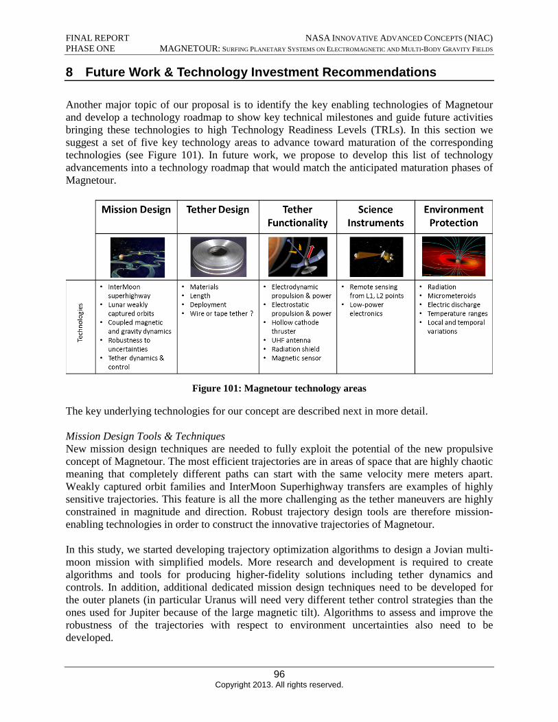
FINAL REPORT NASA INNOVATIVE ADVANCED CONCEPTS (NIAC) PHASE ONE MAGNETOUR: SURFING PLANETARY SYSTEMS ON ELECTROMAGNETIC AND MULTI-BODY GRAVITY FIELDS
8 Future Work & Technology Investment Recommendations
Another major topic of our proposal is to identify the key enabling technologies of Magnetour and develop a technology roadmap to show key technical milestones and guide future activities bringing these technologies to high Technology Readiness Levels (TRLs). In this section we suggest a set of five key technology areas to advance toward maturation of the corresponding technologies (see Figure 101). In future work, we propose to develop this list of technology advancements into a technology roadmap that would match the anticipated maturation phases of Magnetour.
Figure 101: Magnetour technology areas
The key underlying technologies for our concept are described next in more detail.
Mission Design Tools & Techniques New mission design techniques are needed to fully exploit the potential of the new propulsive concept of Magnetour. The most efficient trajectories are in areas of space that are highly chaotic meaning that completely different paths can start with the same velocity mere meters apart. Weakly captured orbit families and InterMoon Superhighway transfers are examples of highly sensitive trajectories. This feature is all the more challenging as the tether maneuvers are highly constrained in magnitude and direction. Robust trajectory design tools are therefore mission-enabling technologies in order to construct the innovative trajectories of Magnetour.
In this study, we started developing trajectory optimization algorithms to design a Jovian multi-moon mission with simplified models. More research and development is required to create algorithms and tools for producing higher-fidelity solutions including tether dynamics and controls. In addition, additional dedicated mission design techniques need to be developed for the outer planets (in particular Uranus will need very different tether control strategies than the ones used for Jupiter because of the large magnetic tilt). Algorithms to assess and improve the robustness of the trajectories with respect to environment uncertainties also need to be developed.
96 Copyright 2013. All rights reserved.

FINAL REPORT NASA INNOVATIVE ADVANCED CONCEPTS (NIAC) PHASE ONE MAGNETOUR: SURFING PLANETARY SYSTEMS ON ELECTROMAGNETIC AND MULTI-BODY GRAVITY FIELDS
Tether design In order to define the tether, several design variables need to be investigated. The most important ones include the tether length, width and thickness. These parameters are critical for producing enough propulsion and power, in particular enough delta-v for the Jovian capture. The materials of the tether must be also addressed. In this study, we assumed aluminum, a standard tether material with good tensile strength and radiation protection properties. More advanced materials should be investigated in future work, like Aracon.
Tether functionality Increasing the functionality of tethers would open up a broader range of mission applications and would increase the benefits of Magnetour. Below is a list of possible innovative tether functions.
Dual-mode electrodynamic / electrostatic tether: This capability is discussed in section 5.1.2.
Hollow cathode thruster: This capability is discussed in section 5.1.1.3.
Radiation shield: In Phase 1, we considered a tether made of aluminum. It follows that the tether itself can provide extra radiation shielding capability and can be coiled around sensitive areas. This technology would be especially useful in the more intense parts of the radiation belts (typically where the magnetic field is the highest so the length can be shorter).
UHF antenna: Electrodynamic tethers have the potential to be used as an antenna and enhance communication at outer planets. In fact, UHF electromagnetic waves are produced when electrons are emitted from the tether back into the plasma. Messages can then be transmitted from the tether by modulating the induced current at the desired frequency. In Phase 2, we intend to understand better this capability and its applications for our Magnetour concept at Jupiter.
Sensor: The tether is also capable of measuring properties of the ionospheric plasma (electron temperatures, ion/electon densities) as a Langmuir probe.
Science Instruments Magnetour relies on nontraditional science orbits to observe the moons, therefore it is necessary to establish performance capabilities, requirements, and possible modifications to key conventional science instruments (such as altimeters, and radio science antennae, accelerometers, visual sensors, etc) develop instruments that will be adapted for our concept. In addition, power produced by an electrodynamic tether at Ganymede and Callisto is likely to be low, in that case the instruments should be adapted to low-power conditions.
Environment Protection Developing technologies to mitigate the extreme outer planet environments should be a priority.In particular, the magnetosphere of Jupiter is the seat of intense radiation that constitutes a significant threat to the spacecraft. Apart from tether radiation shielding and trade-offs in trajectory, studying innovative radiation mitigation techniques is out of the scope of this project. In the future, Magnetour will be able to leverage results from one of the many current radiation mitigation projects. The interaction with the environment is also of critical importance as it provides both powerand thrust for the mission.
97 Copyright 2013. All rights reserved.

FINAL REPORT NASA INNOVATIVE ADVANCED CONCEPTS (NIAC) PHASE ONE MAGNETOUR: SURFING PLANETARY SYSTEMS ON ELECTROMAGNETIC AND MULTI-BODY GRAVITY FIELDS
9 Conclusions
Using numerical simulations that incorporate simplified orbital mechanics and tether dynamics, our preliminary results suggest that a full propellantless concept relying on electrodynamic tethers only is indeed feasible at Jupiter. The concept requires a tether length of at least 20 km at Jupiter. Mass savings can be in the order of 800 kg compared to classical mission concepts and using currently available tether materials. We have developed a preliminary design for a 25-km long tether at Jupiter. The tether is used for capture and lowering the apojove by repeatedly turning on the tether at perijove. Moon flybys are then the most efficient method to raise perijove. A low-energy tour surfing the InterMoon Superhighway and orbiting successively Callisto, Ganymede and Europa requires 5 m/s only, a dramatic improvement over classical patched-conics tour designs. Additional interesting dynamical features can be also found by fully coupling the electromagnetic and gravitational dynamics.
There are many extensions possible of the Magnetour concept that use part or all of the techniques considered in this study:
1. Outer planet cubesats: a tether could be attached to the cubesats to provide propulsionand power without significant mass penalty.
2. Outer planet sample return mission: the Magnetour concept could be augmented byadding a return trajectory leg to the Earth. The sampling of one or several of the moonscould be performed by the tether itself during close flybys.
3. Jupiter observer at low circular orbit: a ‘descope’ Magnetour could simply involve a lowcircular orbit at Jupiter.
98 Copyright 2013. All rights reserved.
FINAL REPORT NASA INNOVATIVE ADVANCED CONCEPTS (NIAC) PHASE ONE MAGNETOUR: SURFING PLANETARY SYSTEMS ON ELECTROMAGNETIC AND MULTI-BODY GRAVITY FIELDS
10 References and Citations
1. “Visions and Voyages for Planetary Science in the Decade 2013 – 2022”, National ResearchCouncil Report, 2011, http://solarsystem.nasa.gov/2013decadal/
2. Lantoine, G., Russell, R. P., “Near-Ballistic Halo-to-Halo Transfers Between Planetary Moons”,Journal of the Astronautical Sciences, Vol. 58, No. 3, 2011, pp. 335-363.
3. Kloster K. W., Petropoulos A. E., Longuski J. M., “Europa Orbiter tour design with Io gravityassists”, Acta Astronautica, Vol. 68, pp. 931-946, 2011.
4. Bokelmann, K. A., Russell, R. P., Lantoine, G., “Exploring Periodic Orbits with ElectrodynamicTethers”, AAS Astrodynamics Specialist Conference, Hilton Head, South Carolina, August 2013(abstract accepted).
5. Kruijff, M., van der Heide, E. J., Stelzer, M., Ockels,W. J., and Gill, E.,“First Mission Results ofthe YES2 Tethered SpaceMail Experiment,”AIAA Paper 08-7385, Aug. 2008.
6. Anon., "Physics of the Jovian and Saturnian Magnetospheres, Highlights of Conference," in Physicsof the Jovian and Saturnian Magnetospheres, John Hopkins University, 1981.
7. Krimigis, S. M. , T. P. Armstrong, A. I. Axford, C. O. Bostrom, G. Gloeckler, E. P. Keath, L. J.Lanzerotti, J. F. Carbary, D. C. Hamilton, and E. C. Roelof, "Low-energy charged particles inSaturn's magnetosphere: Results from Voyager 1," Science, vol. 212, pp. 225-231, 1981.
8. Giorgini, J.D., Yeomans, D.K., Chamberlin, A.B., Chodas, P.W., Jacobson, R.A., Keesey, M.S.,Lieske, J.H., Ostro, S.J., Standish, E.M., Wimberly, R.N., "JPL's On-Line Solar System DataService", Bulletin of the American Astronomical Society, Vol 28, No. 3, p. 1158, 1996
9. Bagenal , F., “Giant Planet Magnetospheres”, Annu. Rev. Earth Planet. Sci., 20, pp. 289-328, 1992.10. Divine, T. N., and Garrett, H. B., "Charged particle distributions in Jupiter's magnetosphere," J.
Geophys. Res., vol. 88, pp. 6889-6903, 1983.11. Garrett, H. B., I. Jun, J. M. Ratliff, R. W. Evans, G. A. Clough, and R. W. McEntire, "Galileo
Interim Radiation Electron Model," JPL Publication 03-006, The Jet Propulsion Laboratory,California Institute of Technology, Pasadena, CA, 2003.
12. Divine, T. N., "Numerical Models for Electron and Proton Distributions in Saturn's RadiationBelts," Jet Propulsion Laboratory IOM 5217-90-029, February 28, 1990.
13. Garrett, H. B., J. M. Ratliff, and R. W. Evans, "Saturn Radiation (SATRAD) Model," October2005.
14. Selesnick, R.S., and Stone, E.C., “Energetic electrons at Uranus: Bimodal diffusion in a satellitelimited radiation belt”, J. Geophys. Res., Vol. 96, No. A4, pp. 5651-5665, 1 April 1991.
15. Mauk, B. H., S. M. Krimigis, E. P. Keath, A. F. Cheng, T . P. Armstrong, L. J. Lanzerotti, G.Gloeckler, and D. C. Hamilton, “The Hot Plasma and Radiation Environment of the UranianMagnetosphere“, J. Geophys. Res., Vol. 92, No. A13, Pages 15,283-15,308, December 30, 1987.
16. Connerney, J. E. P., “Magnetic Fields of the Outer Planets”, J. Geophys. Res., Vol. 98, No. E10, pp.18,659-18,679, 25 October 1991.
17. Connerney, J. E. P., Acuna, M. H., and Ness, N. F., “The Magnetic Field Of Uranus”, J. Geophys.Res., Vol. 92, No. A13, pp. 15,329-15,336, 30 December 1987.
18. Horn, L.J., “Planetary Rings”, in Encyclopedia of Planetary Sciences, J. H. Shirley and R. W.Fairbridge, editors, Chapman and Hall, New York, NY, pp. 602-608, 1997.
19. Sanmartin, J. R., Martinez-Sanchez, M., and Ahedo, E., “Bare Wire Anodes for ElectrodynamicTethers”, Journal of Propulsion and Power, Vol. 9, No. 3, 1993, pp. 353–360.
20. Zanutto, D., Curreli, D., and Lorenzini, E.C., “Stability of Electrodynamic Tethers in a Three-BodySystem,” Journal of Guidance, Control, and Dynamics, Vol. 34, No. 5, Sept.-Oct. 2011, pp.14411456
21. Cooke, D. L., and Katz, I., “TSS-1R electron currents: Magnetic limited collection from a heatedpresheath”, Geophysical Research Letters, Vol. 25, No. 5, pp. 753-756, 1998.
99 Copyright 2013. All rights reserved.
FINAL REPORT NASA INNOVATIVE ADVANCED CONCEPTS (NIAC) PHASE ONE MAGNETOUR: SURFING PLANETARY SYSTEMS ON ELECTROMAGNETIC AND MULTI-BODY GRAVITY FIELDS
22. Katz, I., Lilley Jr., J. R., Greb, A., McCoy, J. E., Galofaro, J., Ferguson, D. C., “Plasma turbulenceenhanced current collection: Results from the plasma motor generator electrodynamic tether flight”,Journal of Geophysical Research, Vol. 100, No. A2, pp. 1687-1690, 1995.
23. Khan B., Sanmartin J. R., “A comparative analysis of survival probability of round wire and thin-tape tethers of equal mass and length against debris impact”, 39th COSPAR Scientific Assembly.Held 14-22 July 2012, in Mysore, India. Abstract B0.2-35-12, p.918
24. Fujii, H.A., Watanabe, T., Kojima, H., Oyama,K., Kusagaya T., Yamagiwa, Y., Ohtsu, H., Cho, M.,Sasaki, S., Tanakaka, K., Williams, J., Binyamin, R., Les Johnson, C., Khazanov, G., Sanmartin,J.R., Lebreton, J-P., van der Heide, J.E., Kruijff, M., Pascal,F., and Trivailo, P., “Sounding rocketexperiment of bare electrodynamic tether system”, Elsevier, Acta Astronautica, Vol.64, pp. 313324, 2009.
25. Personnal correspondence with Dan Goebel.26. Peck M. A., “Prospects and Challenges for Lorentz-Augmented Orbits”, 2005 AIAA Guidance,
Navigation, and Control Conference and Exhibit, San Francisco, CA, USA, 15-18 Aug. 2005.27. Janhunen, P., “Electric Sail for Spacecraft Propulsion,” Journal of Propulsion and Power, Vol. 20,
No. 4, 2004, pp. 763–764.28. Janhunen, P., and Sandroos, A., “Simulation Study of Solar Wind Push on a Charged Wire: Basis
of Solar Wind Electric Sail Propulsion,” Annales Geophysicae, Vol. 25, No. 3, 2007, pp. 755–767.29. Mengali G., Quarta A. A., and Janhunen P.. "Electric Sail Performance Analysis", Journal of
Spacecraft and Rockets, Vol. 45, No. 1 (2008), pp. 122-129.30. Frisbee, R. H., “Advanced Space Propulsion for the 21st Century”, Journal of Propulsion and
Power, Vol. 19, No. 6, 2003, pp.1129-1154.31. Russell, R. P., Brinckerhoff, A.T., “Circulating Eccentric Orbits around Planetary Moons”, Journal
of Guidance, Control, and Dynamics. Vol. 32, No. 2, 2009, pp. 423-435.32. Anderson, R. L. and M. W. Lo, “Flyby Design using Heteroclinic and Homoclinic Connections of
Unstable Resonant Orbits,” 21st AAS/AIAA Space Flight Mechanics Meeting, AAS 11-125, NewOrleans, Louisiana, February 13-17, 2011.
33. Gomez G., Koon W. S., Lo M. W., Marsden J. E., and Ross S. D., “Connecting Orbits and InvariantManifolds in the Spatial Restricted Three-Body Problem,” Nonlinearity, Vol. 17, May, 2004, pp.1571– 1606.
34. Gomez G. and Masdemont J., “Some Zero Cost Transfers between Libration Point Orbits,”AAS/AIAA Astrodynamics Specialist Conference, No. AAS Paper 00-177, Clearwater, Florida,January 23-26, 2000.
35. Anderson R. L. and Lo M. W., “Role of Invariant Manifolds in Low-Thrust TrajectoryDesign,”Journal of Guidance, Control, and Dynamics, Vol. 32, November-December, 2009, pp.1921–1930.
36. Anderson R. L. and Lo M. W., “Dynamical Systems Analysis of Planetary Flybys and Approach:Planar Europa Orbiter,” Journal of Guidance, Control, and Dynamics, Vol. 33, November-December, 2010, pp. 1899–1912.
37. Anderson R. L. and Lo M. W., “A Dynamical Systems Analysis of Planetary Flybys and Approach:Ballistic Case,” The Journal of the Astronautical Sciences, Vol. 58, April-June, 2011, pp. 167–194.
38. Anderson R. L., “Tour Design Using Resonant Orbit Heteroclinic Connections in Patched CircularRestricted Three-Body Problems,” 23rd AAS/AIAA Space Flight Mechanics Meeting, No. AAS13-493, Kauai, Hawaii, February 10-14, 2013.
39. Canalias E. and Masdemont J., “Homoclinic and Heteroclinic transfer Trajectories BetweenLyapunov Orbits in the Sun-Earth and Earth-Moon Systems,” Discrete and Continuous DynamicalSystems – Series A, Vol. 14, February, 2006, pp. 261–279.
40. Canalias E. and Masdemont J., “Computing Natural Transfers Between Sun-Earth and Earth-MoonLissajous Libration Point Orbits,” Touching Humanity - Space for Improving Quality of Life.Selected Proceedings of the 58th International Astronautical Federation Congress, Vol. 63,Hyderabad, India, 24-28 September 2007 2008, pp. 238 – 248.
100 Copyright 2013. All rights reserved.
FINAL REPORT NASA INNOVATIVE ADVANCED CONCEPTS (NIAC) PHASE ONE MAGNETOUR: SURFING PLANETARY SYSTEMS ON ELECTROMAGNETIC AND MULTI-BODY GRAVITY FIELDS
41. Hiday-Johnston L. A. and Howell K. C., “Transfers Between Libration-Point Orbits in the Elliptic Restricted Problem,” Celestial Mechanics and Dynamical Astronomy, Vol. 58, April 1994, pp. 317– 337.
42. Hiday-Johnston L. A. and Howell K. C., “Impulsive Time-Free Transfers Between Halo Orbits,”Celestial Mechanics and Dynamical Astronomy, Vol. 64, 1996, pp. 281–303.
43. Hiday L. A. and Howell K. C. “Impulsive Time-Free Transfers Between Halo Orbits,” AIAA/AAS Astrodynamics Conference, No. AIAA-92-4580, Hilton Head Island, South Carolina, August 1012, 1992.
44. Hiday L. A., Optimal Transfers Between Libration-Point Orbits in the Elliptic Restricted Three-Body Problem. PhD thesis, Purdue University, August 1992.
45. Howell K. C. and Hiday-Johnston L. A., “Time-Free Transfers Between Libration-Point Orbits in the Elliptic Restricted Problem,” Acta Astronautica, Vol. 32, No. 4, 1994, pp. 245–254.
46. Lantoine G. and Anderson R. L., “Evaluation of Initial Guess Strategies for Low-Energy Resonant Flybys,” JPL R&TD Poster Conference, Pasadena, California, November 7, 2012.
47. Lantoine G., Russell R. P., Campagnola S., “Optimization of Low-Energy Resonant Hopping Transfers between Planetary Moons,” Acta Astronautica, Vol. 68, No. 7-8, 2011, doi:10.1016/j.actaastro.2010.09.021.
48. Russell R. P., Lam T., “Designing Ephemeris Capture Trajectories at Europa using Unstable Periodic Orbits,” Journal of Guidance, Control, and Dynamics 30 (2) (2007) 482–491.
49. Ross S. D., Koon W. S., Lo M. W., Marsden J. E., “Design of a multi-moon orbiter,” Paper AAS03-143, AAS/AIAA Space Flight Mechanics Meeting, Ponce, PuertoRico, February 2003.
50. Koon W. S., Lo M. W., Marsden J. E., Ross S. D., “Constructing a low energy transfer between jovian moons,” Contemporary Mathematics, 292 (2002)129–145.
51. Ross S. D., Scheeres D. J., “Multiple Gravity Assists, Capture, and Escape in the Restricted Three-body Problem,” SIAM J. Applied Dynamical Systems, 6 (3) (2007) 576–596.
52. Schroer C. G., Ott E., “Targeting hamiltonian systems that have mixed regular / chaotic phase spaces”, Chaos:An Interdisciplinary Journal of Nonlinear Science, 7(4), 1997, 512–519.
53. Lantoine, G., Russell, R. P., A Unified Framework for Robust Optimization of Interplanetary Trajectories, Paper AIAA-2010-7828, AAS/AIAA Astrodynamics Specialist Conference and Exhibit, Toronto, Canada, Aug 2010.
54. Peláez, J., Bombardelli, C., and Scheeres, D.J. , “Dynamics of a Tethered Observatory at Jupiter,” Journal of Guidance, Control, and Dynamics, Vol. 35, No. 1, Jan.-Feb. 2012, pp. 195-207
55. Pelaez, J. and Lara, M., “Dynamics of Fast-rotating Tethered Satellites,” Monografias de la Real Academia de Ciencias de Zaragoza 32, 2009, pp. 75-83
56. Robinson, W.J., “The Restricted Problem of Three Bodies with Rigid Dumb-bell Satellite,” Celestial Mechanics, Vol. 8, No. 2, 1973, pp. 323–330.
57. Russell, R. “Global Search for Planar and Three-Dimensional Periodic Orbits Near Europa.” The Journal of Astronautical Sciences. Vol. 54, No. 2, 2006, pp. 199-226.
58. Russell, R. P. and Lara, M. “Long-Lifetime Lunar Repeat Ground Track Orbits.” Journal of Guidance, Control, and Dynamics. Vol. 30, No. 4, July-Aug. 2007
59. Martins, J.R.R.A, Sturdza, P., and Alonso, J.J., “The Complex-step Derivative Approximation.” ACM Transactions on Mathematical Software, Vol. 29, Iss. 3, Sept. 2003, pp. 245-262
60. Broucke, R., “Stability of Periodic Orbits in the Elliptic, Restricted Three-body Problem.” AIAA Journal, Vol. 7, No. 6, June 1969
61. Sanmartin, J. R., Lorenzini, E. C., “Exploration of Outer Planets Using Tethers for Power and Propulsion,” Journal of Propulsion and Power, Vol. 21, No. 3, May–June 2005.
62. Yam, C.H., et al., “Saturn Impact Trajectories for Cassini End-of-Mission,” Journal of Spacecraft and Rockets, Vol. 46, No. 2, Apr. 2009.
63. Craig Davis, D., Patterson, C., and Howell, K., "Solar Gravity Perturbations to Facilitate Long-Term Orbits: Application to Cassini," AAS/AIAA Astrodynamics Specialist Conference, Mackinac Island, Michigan, August 2007.
101 Copyright 2013. All rights reserved.

FINAL REPORT NASA INNOVATIVE ADVANCED CONCEPTS (NIAC) PHASE ONE MAGNETOUR: SURFING PLANETARY SYSTEMS ON ELECTROMAGNETIC AND MULTI-BODY GRAVITY FIELDS
64. Campagnola, S., Russell, R. P., The Endgame Problem Part 2: Multi-Body Technique and T-Pgraph, Journal of Guidance, Control, and Dynamics, Vol. 33, No. 2, 2010, pp. 476-486, DOI10.2514/1.44290
65. Jordan, T., “NOVICE: A Radiation Transport shielding code”, 2006.66. Garrett, H. B., and Whittlesey, A. C., “Guide to Mitigating Spacecraft Charging Effects”, JPL
Space Science and Technology Series, J. H. Yuen, Editor-in-Chief, John Wiley and Sons, Inc.,Hoboken, NJ, 221 pages, 2011.
67. Europa 2012 Study Report (Unlimited Release), 2012.
102 Copyright 2013. All rights reserved.