Embed Size (px)
Citation preview

MAGNETOSTRICTIVE DIRECT DRIVE MOTORS
By
Dipak Naik
P.H. DeHoff, P.I.
Semi-Annual Report
January 1, 1990 - June 30, 1990
, NASA Grant NAG 5-1169
Department of Mechanical Engineering & Engineering Science
University of North Carolina at Charlotte
Charlotte, NC 28223
(NASA-CR-IB6O_5) MAGNETOSTRICTIVF P[RECT
_.)RIVL M_]T_,nRS Semiannual _eport, i Jan. - 30
Jun. 1990 (North Carolina Univ.) 7I pCSCL I31
G3137
N_O-Z_d55
https://ntrs.nasa.gov/search.jsp?R=19900019539 2020-05-18T02:02:10+00:00Z

MAGNETOSTRICTIVE DIRECT DRIVE MOTORS
ABSTRACT
This study is concerned with developing magnetostrictive direct drive research motors topower robot joints. These type motors are expected to produce extraordinary torquedensity, to be able to perform microradian incremental steps and to be self-braking andsafe with the power off. Several types of motor designs have been attempted using
magnetostrictive materials. In this report one of the candidate approaches (themagnetostrictive roller drive) is described. The method in which the design will functionis described as is the reason why this approach is inherently superior to the other
., approaches. Following this, the design will be modelled and its expected performancepredicted. This particular candidate design is currently undergoing detailed engineeringwith prototype construction and testing scheduled for mid 1991.

St. No.
NOMENCLATURE
LIST OF FIGURES
LIST OF TABLES
ii-v
vi
vii
1 Introduction 1
2 Construction 1
3 Principles of Operation
4 Expected Performance2-25
4.1
4.2
4.3
4.6
Basic Kinematics 2
Torque ii4.2.1 Drive Rods ii
4.2.2 Structural Stresses and
strains 12
Speed/Acceleration/Step Resolution 154.3.1 No Load Frequency Response 15
4.3.2 On Load Frequency Response 17
Temperature 18
4.4.1 Coil Losses 19
Designing For Wear 20
4.5.1 Effect of Design Variables 21
4.5.2 Effective Wear Control 21
4.5.3 Wear Prediction Technique 22
4.5.4 Analytical Technique 23
4.5.5 Wear Calculations for
Drive Cam 25
Closure 25
APPENDIX: A Preliminary Drawings for Prototype B 41-60
REFERENCES 61

NOMENCLATURE
A = contact area (apparent) in wear calculations
a = distance between end of drive drum to the point of
application of normal forces
alin = linear acceleration (ft/sec 2)
B = magnetic flux density
Bai r = magnetic flux density in air
Bst = magnetic flux density in steel
b = width of rectangular contact area for Hertz contact
stresses
b12 = width of rectangular contact area for drive roller &
drive cam
b23 = width of rectangular contact area for drive roller &
drive shaft
c = width of load support in rolling direction
D = constant in deflection calculations
D1 = diameter of drive cam
D 2 = mean diameter of drive roller
D 3 = diameter of drive shaft drum
Dodr = effective lever arm of drive shaft drum
Ddr = rod lever arm
d = sliding distance in wear calculations
dt = diameter of Terfenol rod
dL = distance over which force F acts
dWH = total energy stored in a steady magnetic field
dincoi I = inner diameter of magnetic coil for drive rollers
docoil = outer diameter of magnetic coil for drive rollers
dair = lenght of air gap
E = Young's modulus
F = Force
Fd = rod drive force
Fpl = spring preload forceFfb = Radial bearing frictional force opposing spring
preload force
Fnpl = Normal force caused by seating of bearing
Frz = Resultant frictional force opposing roller removal in z
direction
Ffpls = Friction force in seating which opposes the preload
Ffpl = Friction force after seating which opposes rollerremoval
Fs = average force of drive roller return spring.
Fz = forces in Z direction
fop = operating frequency of motor
fc = critical frequency of Terfenol rods
fnl = no load frequency of motor
fol = on load frequency of motor
G = drive force on drive shaft drum (ibs)
Gv : required lift
Gr = total possible radial gap
H = material hardness
ii

Hcul = copper loss for electromagnetic coil
Hcu2 = copper loss for Terfenol rod coil
Hcol = core loss for electromagnetic coil
Hco2 = core loss for Terfenol rod coil
h = depth of/wear perpendicular to the contact area
hl = depth of wear at the center of worn area on body 1
h2 = depth of wear at the center of worn area on body 2
ht = total depth of wear at the center of worn area on body 1
and 2
I = electric current
Ii = current in electromagnetic coil
I2 = current in Terfenol rod coil
j = polar moment of inertia
Josc = polar moment of inertia of oscillating members of
motor
Jrot = polar moment of inertia of rotating members of motor
j = film thickness
K m = wear coefficient
KD = K factor in contact stress calculations
KDI = K factor for roller in the drive cam
KD2 = K factor for roller on drive shaft drum
L = Load in wear calculations
idr = length of drive drum
M O = moment acting on drum in inch ibs per linear inch
m = mass of drive roller
Ncam = normal force on drive cam
n = no of times surface passes through loaded area
p = contact pressure in wear calculations
Pc = load for contact stress calculatins
Pdr = total load on drive drum in ibs per linear inch
Pr = load on roller in ibs per linear inch
R = radius of drive drum
rccoil= center point (location of slot) for electromagnet
coil for drive rollers
rincoil = inside radius of electromagnet coil for drive
rollers
rocoil = outside radius of electromagnet coil for drive
rollers
Rc = radius from centre of motor to centre of drive roller
rdr = drive drum radius
Rai r = reluctance of air gap in magnetic circuit
Rcoill = electrical resistance of electromagnetic coil
Rcoil2 = electrical resistance of Terfenol rod coil
rrod = rod lever arm (in)
r r = drive roller mean radius
S = core cross sectional area
Sair = cross sectional area of air gap
Sst = cross sectional area of steel core
s = amount of drive roller arc length travel required during
the return stroke.
Tdr = drive torque (ft-lbf)
iii

T = Temperature
Top = time period of motor
Tnl = no load time period of motor
Tol = on load time period of motor
tdr = thickness of drive drum
t = time-
tl = time of first observation
t2 = time of second observation
U = rolling velocity
Us = sliding velocity
V = Velocity
Vm = magnetomotive force
W = wear
W r = rate of wear
W 1 = wear at time tl
W 2 = wear at time t2
Yr = radial deformation of drum
Greek Alphabets:
= angular acceleration (radians/sec 2)
_en = environmental effects
_nl = no load angular acceleration of motor
_oi = on load angular acceleration of motor
= geometric effects
@ = angular resolution of motor
V = poisson's ratio
= cam angles
= magnetic flux
= roller angle
_f = finish factor
= electrical resistance in ohms
_o = permeability of free space
_s = coefficient of sliding friction
I = constant
_F z = sum total of forces in Z direction
_J = total polar moment of inertia of oscillating and
rotating members of motor
_Josc = total polar moment of inertia of oscillating members
of motor
_Jrot = total polar moment of inertia of rotating members of
motor
_Loss = total heat loss in motor
iV
ALdr = expansion of drive rods
Ardr = total radial deformation of drive shaft drum, drive
rollers and drive cam
Arr = radial def%rmation of drive roller
ALdr = expansionof drive rods
_cmax = Maximum contact stress
Abbreviations/Acronyms:
rpm = revolutions per minuteCW = clockwise
CCW = counter clockwise
AWG = American wire gage
V

Sr. No .
1
2
3
4
5
6
7
8
9
i0
ii
Ii
LIST OF FIGURES
Ti__m]e Page No.
Magnetostrictive Direct Drive Motor
Top View of MotorFront View of Motor (Section A-A)
Locking roller Drive Details
Output Shaft Drum
Drive Drum
Functional Operation of Roller Drive
Free Body Diagram of Rollers
26
27
28
29
3O
31
32
33-34
Guide Spring Details 35
Regions of Backlash, Dead Zones and Hysteresis36-38
Performance Characteristics of
FSZM Terfenol Rods 39
Effect of Operational Variables on Wear
Rate 40
vi

1
2
3
4
5
i0
Ii
12
13
LIST OF TABLES
Ti_ P_ge No.
Radial Defo_nation of Drive Drum 13
Radial Deformations of Drive Rollers 14
Radial Deformations of Drive Cam and Drive
Shaft Drum 14
Cumulative Radial Structural Deformations 14
Contact Stresses: 15
a. Drive Roller In Drive Cam
b. Drive Roller On Drive Shaft Drum
Polar Moment of Inertia (Josc) of Oscillating
Members 17
Polar Moment of Inertia (Jrot) of
Rotating Members 18
Polar Moment of Inertia (_J) of Oscillating
and Rotating Members 18
On Load Angular Accelerations and Frequency
Response 18
Electromagnet Coil Specifications 19
Coil Wire Specifications 19
Terfenol Rod Coil Specifications 19
Heat Losses in Coils 20
vii

NASA/UNCC: NAG 5-1169
MAGNETOSTRICTIVE ROLLER DRIVE MOTOR
John M. Vranish Dipak P. Naik
NASA/Goddard Space Flight Center
i. INTRODUCTION
Robot arms in space are currently powered by low torque,
high speed electric motors which use transmissions as a means
of torque multiplication and which utilize brakes as a safety
device when the power is off. Direct drive control, though
highly desirable, is not presently practical. The addition ofthe transmission hardware and brakes makes the system bulky
and inefficient. Also, the fact that DC motor servo control
is used, results in limit cycling. Motors based on
magnetostrictive principles appear to hold promise in
alleviating these problems and to allow for unprecedented
precise microradian steps, safety and agility. Several
concepts based on magnetostrictive drives have been
attempted, all with varying degrees of success. In this paper
the magnetostrictive roller drive motor will be introduced
and its means of functioning explained. The reasons why this
new design is inherently superior to earlier magnetostrictive
motors will be made clear.
2. CONSTRUCTION
Fig. 1 illustrates the motor concept. It essentially consists
of magnetostrictive drive rods which impart a torque to the
roller locking mechanism which, in its turn, transfers the
torque to the output shaft. The torque produced by the
magnetostrictive rods is oscillatory while that emerging from
the output shaft is unidirectional (but reversible). Figs. 2
and 3 show the proposed design in full scale and give an idea
of its size and complexity. The locking roller drive is the
heart of the motor and Fig. 4 shows details of this
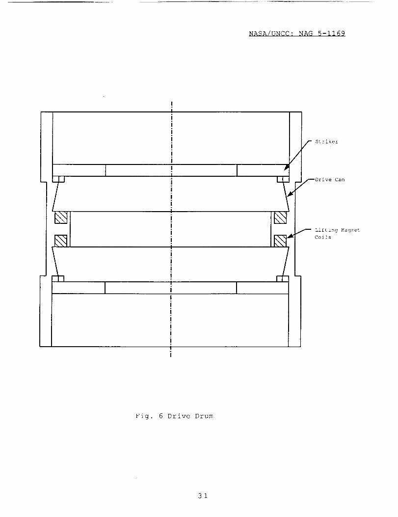
mechanism. Figs. 5 (drive shaft drum) and 6 (drive drum) show
the main components.
3. PRINCIPLES OF OPERATION
Figs 2 and 3 show a full scale view of the proposed motor
design. We expect approximately 60 ft-lbs torque with no-load
speeds on the order of I0 rpm from the motor.
Fig. 7 illustrates the functional operation of the
roller drive. The illustration shows clockwise drive shaft
rotation. Each of one pair of magnetostrictive rods (A)
expands approximately 0.001in'in. with great force, exerting
2 ksi ( 500 ibs each for a 0.55 in diameter rod) under the
influence of a magnetic field. The opposing rods (B) contract

NASA/UNCC: NAG 5-1169
approximately 0.001 in./in, each. Thus we have a rotational
motion of the drive drum. This drive drum is coupled to the
drive shaft drum by conical rollers. These rollers are
lightly preloaded so there is no backlash between the drive
cam and the drive shaft drum. As the drive drum rotates CW,
the CW drive rollers try to roll up the CW drive cam on the
drive drum; but are immediately pinned between the drive
shaft drum and the drive cam. And since tan _ < _the
frictional force preventing sliding builds up instantaneously
so the rollers lock. This locking sets up reaction forces in
the drive drum and the drive shaft drum. These forces, in
turn, create the friction forces on the drive shaft drum
which constitute the source of motor torque. At the same
time, the magnets above the CCW rollers are activated.
Following this, the CCW rollers first roll, disengaging from
both the drive cam and the drive shaft drum, and then are
each pulled up against the magnetized plate. Thus, a
preferential CW torque and motion is established. When the
magnetic field in the expanding rod set (A) collapses, the
system returns to neutral and the cycle can start again
(except that the CCW rollers are effectively
nonparticipatory) . When the magnetic field is excited at high
frequency (on the order of 400 Hz) the system cycles in a
rapid ratcheting motion and we get relatively high rpm (i0
rpm for a single stage motor) . When the above procedure is
followed using the magnetostrictive rod pair (B) as the drive
source, and another set of rollers which are stationed
underneath the first s_t of conical rollers. The drive cams
on the drive drum are set up so that locking takes place in
CCW motion and we get CCW ratcheting motion.
4. EXPECTED PERFORMANCE
In this section we will examine the expected performance of
the motor. We will first investigate how the system works
kinematically. This will ensure that the basic motion
sequence of the device is correct. We will next analyze the
device to see that it will produce the required torque. Then
we will estimate its potential with respect to speed,
acceleration and step resolution. This, in turn, will be
followed by an estimation of the power, efficiency and
operating temperature of the system. Finally, wear and
longevity will be estimated.
4.1 Basic Kinematics
In this section we will examine the basic kinematics of the
motor. We will go through all the steps of the drive cycle
first in one direction and then in the other, tracing the
movements of all critical parts as we go.
We will begin by driving the motor clockwise. For the
motor to operate with such small drive strokes, components
2
NASA/UNCC: NAG 5-1169
must be kept in contact and forces in balance at all times
with backlash, hysteresis and dead zones reduced to a
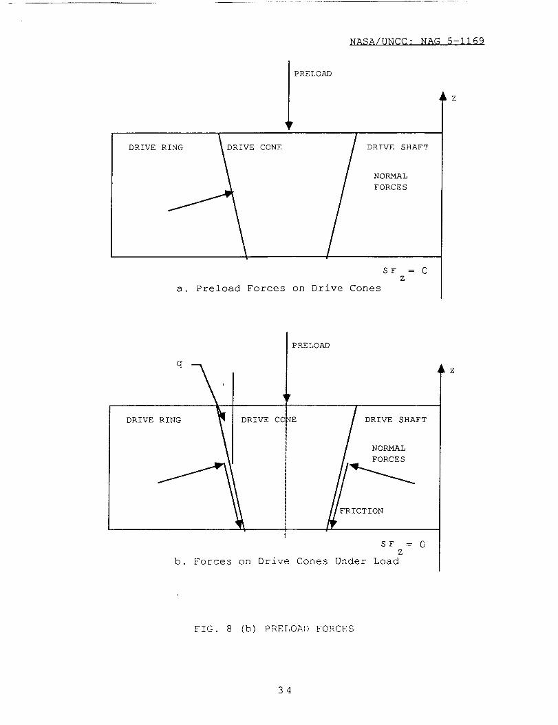
minimum. Fig. 8 (a) and (b) shows the preload forces in the
X-Y plane. The CW rollers remain in contact with both the
drive cam and the drive shaft drum throughout the power
stroke. Each roller rolls initially, causing structural
deformation, until the driving force builds up to equal the
torque opposing the motor shaft. Then the CW rollers lock the
drive cam and the drive shaft drum together and the motor
overpowers the torque load on its shaft. During the
relaxation stroke, the drive drum rotates CCW relative to the
drive shaft drum. This forces the CW rollers to rotate CCW
until all deformations are relieved and the forces shown in
Figs. 8 (a) and (b) return to preload levels This also
places each roller in contact with its guide spring/bearing
(Fig. 9). As the drive drum continues to move CCW, each guide
spring/bearing pushes its respective roller before it. These
rollers, however, are preloaded against the drive cams and
the drive shaft drum, so they roll throughout the return
stroke. This leaves them each in contact with the drive cams
and drive drum so backlash and dead zones are minimized for
the next power stroke. When we choose to reverse directions,
we release the magnets above the CCW rollers and excite those
above the CW. We then excite the magnetostrictive rods to
perform a CCW power stroke. The CCW rollers respond to their
preload springs and move down in the Z direction until they
contact the cams of the drive drum and the drive shaft drum,
where they begin the process of first rolling to build up
torque forces and then locking the drive drum and drive shaft
drum together. The CW rollers roll until all deformations and
forces are reduced to preload minimum. They then are pulled
up against their respective magnets and CCW ratcheting can be
performed. But how do we keep this balance of forces and
minimum backlash and dead zones throughout the motor life,
when wear is occurring and when the drive drum and the drive
shaft drum are slightly out of round?
A second cam surface is used along with vertical preload
springs to provide an independent suspension for each of the
rollers. Thus, they can individually stay in contact with the
drive drum cam and the drive shaft drum, minimize backlash
and maintain balance of forces despite wear and anomalies in
manufacture. Again, tan _ < _ so the drive rollers will not
displace in the Z or vertical direction no matter how much
force is applied. For the CCW rollers, separation is desired
throughout the power and relaxation strokes. Without this
separation, a relaxation stroke would not be possible. Thus,
electromagnets are used to lift the CCW rollers clear of
contact with the drive drum cams and drive shaft drum during
the CW ratcheting process. For CCW ratcheting, we excite the
electromagnets over the CW rollers and relax those over the
CCW rollers. We will now identify areas of dead zones, back
lash and hysteresis.

NASA/UNCC: NAG 5-1169
In Fig.10, we identify the regions of back lash, dead
zones and hysteresis. In Fig. I0 (a), we trace the contact
stresses build-up on the drive roller throughout the drive
stroke. When the drive stroke is just beginning, the stress
on the drive roller is that caused by the downward preload
and is minimal. As the power stroke continues, the drive
roller rolls and deforms both itself and the surrounding
structure (see also Fig.10 (b)) until the torque opposing the
motor is equalled (see Fig. I0 (c)) . At this point, the drive
rollers stop rolling, they lock the drive cam and the drive
shaft drum together and the drive shaft turns. The graphs of
Figs.10 (a) and I0 (b) show the contact stresses and
deformations associated with maximum torque. We have set as a
rule-of-thumb that this should occur before one half of the
stroke because we want reasonable movement of the load even
under high torque conditions. The portion of the drive stroke
during which the rollers roll and the structure deforms up to
the point of movement of the drive shaft represents the dead
zone. The extent of the dead zone is proportional to the
torque load of the motor. For a low torque loading, the dead
zone will be small, the stroke relatively long and the speed
relatively high. During the return stroke (Fig.10 (a) and
(b)), the drive rollers first roll CCW to relieve the forces
and deformations until each is in contact with its guide
spring/bearing. At this point, this spring, which is attached
to the drive cam, forces the drive rollers to follow the
drive drum and, together with the Z direction preload
springs, forces contact between each of the drive rollers andthe drive cam and drive shaft drum. Thus the drive rollers
roll CCW throughout the return stroke. And, because of the
shape of the cams they remain in the same relative Z position
throughout. In certain circumstances, where speeds are high
enough, the inertia of each drive roller during the return
stroke loads its guide spring/bearing slightly, and opens a
tiny gap between the drive roller and the drive cam and drive
drum. The drive roller preload spring forces each drive
roller in the Z direction until contact is re-established.
But this places the roller on a slightly different point on
its drive cam and leaves each guide spring/bearing with a
slight preload. This, in turn, loads forces and deformations
into each roller, drive cam and drive shaft drum. But this
preload, in turn, improves the system frequency response
until the gap no longer occurs. This phenomenon is termed
"walking" and the difference between the forces and
deformations in the system under this condition and normal
preload is hysteresis. When we go from CW drive to CCW drive,
this hysteresis is negated. Under starting conditions of
normal preload (no walking effects), there is no inherent
backlash. Both sets of rollers are at preload and the magnets
above one set of rollers pulls them up and the CCW drive
rollers begin to generate torque and deformations
immediately. Where walking effects have occurred (say during
CW operation) and we begin operating CCW, the following

NASA/UNCC: NAG 5-1169
sequence occurs. First the magnets above the CW rollers are
excited and those above the CCW rollers relaxed. The CCW
rollers are moved by their preload springs so that each
engages its drive cam and the drive shaft drum at normal
preload. The CW rollers, however, are each held in place by
residual "walking" forces from its guide spring/bearing and
cannot respond to its lifting magnet. These residual forcesmust be relieved and the rollers lifted before the motor can
ratchet in a CCW direction. As the CCW power stroke begins,
the CCW rollers begin to roll immediately, building up
deformations and torque in the system. At the same time, the
CW rollers roll down their drive cams (rotating CCW) and
relieving the stresses caused by the walking effect. Once
normal preload levels are reached, their magnets pull them up
and normal CCW operation commences. The period during which
the walking effect forces exceed the forces caused by the CCW
rollers is a period in which no CCW motion or torque can be
generated and adds to the backlash.
We will also briefly examine how the system behaves
kinematically during the return stroke (say CW) . Under these
circumstances, the Terfenol rods are returning CCW to neutral
and the CCW drive rollers are disengaged. In this instance,
each CW roller will rotate CCW because of its preload contact
with its drive cam and the drive shaft drum. Because of the
directional difference of rotation between the drive drum
cams and the drive shaft drum and because of the reverse
slope of the drive cams, the drive roller will translate
radially inward as it rotates, thereby breaking contact with
the drive shaft drum (at the rotational speeds involved,
centrifugal force can be neglected). At the same time, each
drive roller guide spring/bearing is being flexed and its
return force increased until an equilibrium is reached.
Because the translations are so minuscule (in the _ in.
region), the forces on the return spring are very small (near
preload) and wear and energy loss is minimum.
We will now examine the system which disengages the
trailing rollers (CCW drive rollers in the case of CW motor
rotation). Figs. 2, 3 and 4 show the drive rollers and
lifting magnet system in full scale. Preliminary drawings
listed in Appendix: A show the details. From the above
Figs., we see that as the drive stroke moves clockwise, each
trailing (CCW) roller rolls free of drive deformation and is
held in contact with the drive cams and drive shaft drum only
by its preload spring Thus when the lifting magnets above
are activated, the striker (star wheel: Fig. 3) preload
springs is pulled towards its activated windings in the drive
shaft drum. This star wheel impacts each of the trailing
rollers on a one by one basis, breaking them loose three at a
time until all the trailing rollers are lifted free of
contact from their drive cams and the drive shaft drum. It
takes considerable current to lift the rollers (2 amps) ; but
5

NASA/UNCC: NAG 5-!!6_
once they are broken loose and the star wheel is in contact
with the drive cam with the magnetic flux lines closed, this
drops to less than 200 milliamps with power requirements on
the order of milliwatts. In this configuration the system
acts as a single direction ratcheting device biased towards
CW rotation. To reverse direction of rotation we release the
CCW drive rollers, activate the lifting magnets above the CW
rollers and start ratcheting the motor CCW. The CCW rollers
engage the drive shaft drum and drive cams and start to
ratchet torque output in a CCW direction. In the first
portion of the first stroke of the drive rods, the CW rollersroll free of their drive stroke structural deformations, are
lifted by their corresponding magnet and the system acts as
CCW-biased ratcheting device.
Figs. 4 show in detail how the lifting system is
constructed. The lifting magnet coils are embedded into the
drive shaft drum. Above each set of coils is a star wheel
which is positioned above its respective coil such that when
the coil is activated the magnetic flux attracts the star
wheel towards itself with considerable force. This star wheel
is held apart from the drive drum by flat springs which are
stiff in rotation about Z; but compliant in the Z transverse
direction. A disc stand off enables the gap between the star
wheel and the drive cam to be set with precision and allows
the preload forces in each spring to also be set with
precision. Magnet wire (AWG 23) is used and flux lines follow
the circuit shown in Fig. 4. A hole is drilled through the
center of each drive roller and the roller is fitted over a
stainless steel shaft. The shaft is modified to include the
addition of radial preload springs (Fig. 9) and the roller is
modified to facilitate the addition of a preload spring
(Fig.9) . Thus, the position of the roller relative to the
drive drum cams and drive shaft drum is set along with the
forces on those cams and the several compliances (CW, CCW, Z
and structural stiffness) of the roller. Also, the
coefficients of friction (rotation of the roller about the
shaft and sliding up and down on the shaft require a low
coefficient of friction and the contact between the roller
and the drive drum cams and drive shaft drum requires a high
coefficient of friction) are set.
We will now determine whether the magnet can lift the
rollers with a sufficient margin of safety. In determining
this, we will first determine how high we must lift the
roller. We will next determine the forces that must be
overcome. Finally, we will examine the power required to
lift and hold the roller so that we can see if the solution
is practical for extended use.
In determining how high we must lift the rollers we
start with the radial errors in manufacturing between the
drive cam, the drive rollers and the drive shaft drum. We can
assume that these can be held to 0.002 in. These errors
NASA/UNCC: NAG 5-1169
mandate that the rollers be able to ride up and down
independently to correct during rotation. We also assume that
wear will occur and we allow 0.005 in radial wear. This seems
very generous in light of the size of the rollers, their
limited rotation and practically nonexistent slip under load
and the small number of total rotations the motor must
perform (because it is a high torque direct drive device).
Since we have a I0 degree cam angle on the drive cam, we
have.
GrGv .... (I)
2tan
Where:
Gv = required lift
Gr = total possible radial gap (manufacturing
errors and wear, 0.007in) .
= cam angles (i0 deg) .
We calculate Gv =0.006 in (initial setting) and 0.020 in
(after maximum wear). Since our star wheel must lift all
rollers some minimum distance to ensure the drive
disengagement of each (say 0.005 in.), our gap is 0.025 in.between the star wheel and the drive drum.
We will now determine the forces to be overcome in
lifting the rollers. We have the weight of the drive rollers
(0.0152 ibs) . For reasons that will be explained later in the
section on frequency response, we set the radial preload in
the direction opposite the direction of drive very light (say
0.25 ibf) and the radial preload in the direction of drive
very stiff. Similarly, we set a 0.25 ibf radial preload
forcing each roller towards the center of the motor. Thus,
our net radial preload inside the hole is 0.35 ibf and the
coefficient of friction between these springs and the roller
is that of a bearing (say 0.2) with a frictional resistance
to lifting of 0.0751bf. We know that the weight of each
roller is 0.0152 ibs. And, since we want the rollers to stay
in place during the 12 "g" launch environment, we require a
vertical preload of
12 (0.0152) ibf - 0.075 lbf = 0.1074 lbf ... (2)
this means that the vertical preload spring for each roller
is 0.1074 ibf. The star wheel must overcome several forces to
include:
a. 18 vertical preload springs 0.1074 lbf (1.933 lbf) .
b. 18 radial preload frictional forces 0.075 ibf (1.35 ibf) .
c. 18 sets of frictional forces caused by the rollers seating
against the drive cams and the drive shaft drum (see Fig.10
and equations shown below) 0.041 ibf (0.489 ibf) for _s =

NASA/UNCC: NAG 5-1169
0.3; 0.048 ibf (0.575 ibf) for _s = 0.5; 0.0525 ibf (0.944
ibf) for _s = 0.75.
During Seating,
X Fz = 0
Fpl - Ffb - 2Fnpl sin _ - 2Ffpls cos _ = 0
Fpl - Ffb
mnpl - 2(sin _ + _s cos _)
... (3)
During removal,
Frz = FpI - Ffb - 2Fnpl sin _ + 2Ffpl cos
Ffpl = _sFnp]
_sCOS ¢
Frz = 2(Fpl - Ffb)sin # + _sCOS
... (4)
... (5)
Fpl = spring preload force
Ffb : Radial bearing frictional force opposing spring
preload force
Fnpl = Normal force caused by seating of bearing
Frz : Resultant frictional force opposing roller removal in z
direction
Ffpls = Friction force in seating which opposes the preload
Ffpl : Friction force after seating which opposes roller
removal
= Roller angle
Adding a.,b., and c. together we get the total force required
by the star wheel to release all 18 rollers. 3.772 Ibf for _s
: 0.3, 3.858 ibf for _s = 0.5 and 4.227 Ibf for _s = 0.75
(which is extreme). We need a force on the star wheel of 20
ibf at 0.025 in gap to provide a 5:1 safety factor in
lifting. This is actually very conservative as we lift the
rollers one by one and the air gap will be somewhat less than
0.025 in.
G v =
We will now design the electromagnetic lifting mechanism
Gr(¢ : i0 o) ...(6)
2tan
8

NASA/UNCC: NAG 5-1169
2tan i0 °
= 20 E -03 inch maximum gap
For initial setting
= 6.0E -03
We use tool steel because we want the lifting magnet
structure to add to the structural rigidity of the drive
drum, to enhance simplicity to reduce the different kinds of
metals involved and because our magnetic reluctance path
lengths are short compared to the gap so there is little to
be gained by going to special magnetic materials. We must
overcome 4.227 ibf to lift the 18 rollers in the extreme
case.
B2stdW H = FdL - SdL [i] ... (7)
2Bo
Where,F : force
dL : distance
dWH = total energy stored in a steady magnetic field
S : core cross sectional area
Bst = magnetic flux density in steel
_o = permeability of free space (4ZE-7 Henrys/meter)
B2st
i.e. F - 2m O Sair [i] ...(8)
Bst in saturation is 1.4 Wb/m 2
We will use Bst = 1.0 Wb/m 2 to keep below the knee of the B-H
curve
i.e. F = B2stsai r
2_o
= 5 Ibs on one gap or I0 Ibs total ...(9)
B 2 Sair = 2 (4.448 N) (5 ibf) 4z E-07
: 5.589 E-05 Wb2/m 2 ... (i0)
Sair = plate area2
Z((21/16) 2 - (13/32) 2 )
= 2(39.37)2
: 1.5785 E-03m 2
m 2
... (11)

NASA/UNCC: NAG 5-1169
Bair = 0.18818 Wb/m 2
And,
= Bair Sair
= 2.9704 E-04 Wb
= Bst Sst
i.e. (l.0Wb/m 2) Sst = 2.9704 E-04 Wb
i.e. Sst = 2.970 E-04 m 2
We require 0.125 in thickness in return flange for strength
Kdinco_!(0.125)
Sst = (39.37)2
: 2.9707 E-04 m 2
min. dincoil = 1.172 in (locates inner diameter of coils.
Outer diameter docoil = 2.225 in ( and represents the
furthest out we can go and still retain structural strength
in front of the rollers.)
rccoil = center point (location of slot)
2K(rccoil 2 - rincoil 2) = _(rocoil 2 - rincoil 2)
(rQcoil 2 + rin¢oil 2)
rccoil = 2
rccoi! = 0.97152 in (as located in Fig. 4)
dairRai r = At/Wb
_oSair
dair : 0.02 in
Rair
2 (0. 025)
39.37(4K E -07)1.5785 E -03
Rai r = 6.4025 E 05 At/Wb
Vm = _ Rair = 190 At
We measure the pocket for coils
0.5 in = docoil - dincoil
0.2 in high
We use 23 AWG wire, 0.025 in dia with heavy insulation rated
at 3.15 ampers. "
0.5- 20 turns per row
0.025
160 turns 0.75 = 120 turns
120 I = 190 At
I = 1.58 ampers for I0 lbf
i0
NASA/UNCC: NAG 5-1169
Since F _ B 2
& B _ I;
we have,
F _ 12
for I = 2 amps,
(2.OO)F : i0 _ 2
: 16 ibf, using 2 amps
4.2 Torque
In this section we will see if the motor can deliver the
large torque expected of it. We will do this by first
examining the magnetostrictive drive rods to see if they can
deliver the required force. We will then examine the
structure, both geometry and materials characteristics, to
see if it can sustain the forces of the rods and convert them
to torque to the load without major parasitic losses in
deformations.
4.2.1 Drive Rods.
The magnetostrictive rods are made of Terfenol-D,
Tb.3Dy.7Fel.93 Free Stand Zone Melt (FSZM) and their
performance characteristics are shown in Fig.ll. We will
design the motor for 60 ft-lbs torque. Using the motor
configuration shown in preliminary drawings in "Appendix A",
we know that we need a force of:
F d = Dd r
where:
F d : rod drive force
Tdr : drive torque (60 ft-lbf)
Ddr = rod lever arm (1.5 in)
...(12)
We get a force per rod of 475.17 lbs. This requires
using a Terfenol rod of 0.55 in. dia. exerting a force of 2
ksi, which, as we can see from Fig. Ii, is well within the
state-of-the-art.
We will now explore the structural deflections generated
in reaction to the torque. From Fig. 7, we can see that the
forces F which are imposed on the drive shaft drum by the
drive rollers compress the drive cam along 18 equally spaced
radial directions and thus no net compression of the drive
cam takes place. (There will be local indentations). The
forces Nca m act outward on the drive cams. And, since these
also are equally spaced, the drive drum is stretched; but
(except for local deflections) the drive drum does not deform
in an oval pattern. We know:
ii

NASA/UNCC: NAG 5-1169
Tdr = G * Dodr... (13)
where:
Tdr = maximum drive torque (60/40/30 ft-lbs)
G = drive force on drive shaft drum
(213.9/142.59/i06.94!bs)
Dod r = effective lever arm of output drum (3.3661417 in)
And we know that _, the drive cam angle = I0 deg. Thus,
G (14)Nca m - ...
sin
Ncam = 1231.7707/821.18046/615.88535 ibs for 18 rollers
OR
68.431705/45.621137/34.215853 ibs per roller
4.2.2 Structural Stresses and Strains.
We know that as the motor drives, the drive rollers roll
slightly, deform and the drum stretches until the structural
reactions balance the torque forces. We desire that this
equality of forces occur before the stroke reaches the half
way point so that we can get useful motion at maximum torque.
At maximum torque, our structural deformations are:
' __MCL_ . C!4-P41r--, C3Ca2_ - C4Cal +
Yr = 2D13 Cll 2D_2 Cll... (15)
Where, D and k are constants which are defined as follow
m =
Etdr 3
12(i.0 - V 2)
3(1.0 - v 2)
k : ( Rdr2tdr2 **0.25
C3 : sinh (_idr) sin (lldr)
C4 = cosh(kldr) sin(kldr) - sinh(kldr)COS(_idr)
CII = s inh2 (kldr) - sin 2(kldr)
C14 : s inh2 (kldr + sin 2 (lldr)
Cal = cosh_(idr- a)cos_(idr - a)
Ca2 = coshl(Idr - a)sinl(ldr- a)
+ sinh_(id r - a)cos_(idr - a)
a = distance from edge of drive drum to location of normal
forces on drive drum
12

NASA/UNCC: NAG 5-1169
Yr = radial deformation of drum
Pdr = total load on drum in ibs per linear inch
M o = moment acting on drum in inch ibs per linear inch
tdr = thickness of drive drum
Rdr = radius of drive drum
idr = length of drive drum
v = Poisson's ratio
E = Young's modulus
KDI -DID2
D1 - D2for roller in drive cam
D3D2
KD2 - D3 + D2 for roller on the drive shaft drum
b = 2.15(Pd_. kD) *'1/2
b)Ar r = r r (I.0 - sin(arccoS(_r ))
... (16)
where,
b = width of rectangular contact area
D 1 = diameter of drive cam
D 2 : diameter of drive roller
D 3 = diameter of drive shaft drum
The total flexure of the structure is the algebraic sum of
value given by equation (4) and two values given by equation
(5) one each for flexure of drive roller for contact with
drive cam and with drive shaft drum respectively and radial
flexure of drive cam and drive shaft drum.
The summary of the results are shown in Table 1 to 4:
Table I: Radial Deformations of Drive Drum
Torque (ft-lbs) Drum thickness (in) _eformation (_-in)
30 0.6125 9.8391435
40 0.6125 13.119165
60 0.6125 19.680127
13

NASA/UNCC: NAG 5-I16_
Table 2: Radial Deformations of Drive Rollers
Torque (ft-lbs)
30 40 6O
I) Roller inside drive cam
2) Roller on drive shaft drum
Deformations (_-in)
14.3231 19.00 28.6477
3.15956 4.21275 6.3202
Table 3: Radial Deformations of Drive Cam and Drive
Shaft Drum
TQrqu_ (f%-ibs)
30 40 6O
a) Drive cam
b) Drive shaft drum
D@f©rmations (_-in)
10.8081 14.4071 21.6158
0.035483 0.04658 0.070958
Table 4: Cumulative Radial Structural Deformations
TQrque (ft-lbs) Drum thickn@ss (in) DeformatiQn (_-in)
30 0.6125 3.1653870
40 0.6125 50.785595
60 0.6125 76.334793
We calculate that the allowable flexure in a half stroke is
157.1 _-in. Thus, deformations appear to be manageable.
(local deformations remain to be computed using finite
element techniques).
The basis of the initial deformation calculations is:
Rdr* ALdr * sinArdr = -_-
... (17)
whe re :
Ardr = flexure of drum, rollers and drive cam.
(146.52 E-06 in)
Rdr : drive ring radius (1.6875 in from scale drawing)
ALdr = expansion of drive rods
: angle of drive cam (I0 deg)
14

NASA/UNCC: NAG 5-1169
(The 1/4 factor is because we are using 1/2 stroke and
because the rollers roll 1/2 the distance of the stroke)
The contact stresses between drive roller, drive cam and
drive shaft drum are shown in Table 5 and can be calculated
through following equation.
_cmax : 0.591[EPc/KD] 1/2
Whe re,
_cmax = Maximum contact stress
Pc = load in ibs/inch
Table 5: Contact Stresses
Drive Roller Position
a. Inside drive camb. On drive shaft drum
Torque (ft-lbs)
30 40 60
Contact Stresses (ksi)
27.62 31.89 39.06
58.81 67.90 83.16
The elastic limit for high strength alloy steel S.A.E. 52100
is 175-240 Ksi, thus the design is safe.
4.3 Speed/Acceleration/Step Resolution
In this section we will estimate the expected speed,
acceleration and step resolution of the motor.
We will begin by first estimating the no load speed
requirements of the motor. These requirements determined, we
will examine the ability of the motor design to meet these
requirements starting with the frequency response of the
drive rods. We will then calculate the no load inertial
limitations of the device to be allowed by the frequency
response of the drive rollers and finally the trailing
rollers.
4.3 .i No Load Frequency Response
We will begin by estimating the maximum no load speed.
Since this is a direct drive motor with large torque, our rpm
can be relatively low and still move the load at reasonably
high speeds. For example, 20 rpm at the joint of a 24 in arm
will move the tip of that arm at 50 in/s which is excessive
for space and fast even by industrial standards. Let us see
if we can obtain 20 rpm. Our drive cycle is:
Drive stroke Top/4
Return Top/4
15

NASA/UNCC: NAG 5-1169
For a total drive cycle of Top/2
Where Top is the period of the operating frequency f (or Top
= I/fop).
The angular movement we get per drive stroke is
ALdr8=
trod
where
ALdr = expansion of drive rods
fro d = rod lever arm (I.00 in)
8 = 2.0 E -03 radians
... (18)
To achieve our desired angular speed, we require a steady
state operating frequency of.
...(19)fop = 60*8
For 20 rpm f calculates to 437 Hz.
The critical frequency fc for efficient operation of the rods
is.
fc //l_Hz [2]= dt 2
... (20)
where d t is the Terfenol rod diameter in inches. For our rod
diameter of 0.55 in. we get an fc of 352 Hz. However, if we
laminate the rod into four equal segments 0.275 in., we get
fc of 1.4 KHz which is acceptable. Thus rod diameter is not a
problem.
No load inertial limitations involve the rods, the drive drum
and the drive and trailing rollers. We can neglect the
output drum and output drive shaft because they store kinetic
energy in the no load condition.
The frequency response of motor under no load depends on
the inertia of oscillating parts of motor. The inertia of
oscillating parts, torque and angular acceleration of motor
are related by the following well known equation:
Where,
_Josc
Tdr
Tdr = _Josc _nl ... 21)
= Polar Moment of Inertia of Oscillating
Members of Motor (lb ft sec 2)
: Torque (60 ft ibf)
16

NASA/UNCC: NAG 5-1169
(Znl = No Load Angular Acceleration of Motor
(rad/sec 2 )
The individual polar moment of inertias calculated from the
data taken from preliminary drawings listed in "Appendix A"
is shown in following table.
Table 6: Polar Moment of Inertia (Josc) of Oscillating
Members
Josc (ft ib sec 2)
Member Each No/StaQe Total
Rollers 7.4238E-06 36 2.67256E-04
Preload Plates 0.0137712 2 0.0275424
Drive Drum 0.1263266 1 0.1263266
E Josc = 0.1541362
Substituting the values of _Josc and Tdr in equation
(21), we get
_nl = (389.26/259.51065/194.63299)rad/sec 2 for 60/40/30 ft-
ibs torque.
The angular movement @, angular acceleration _nl and time Tnl
are related by following equation:
0 : 0.5 _nl Tnl 2 • --(22)
Where,
0 = 2.0 E -3 rad
From equation (22) we have,
Tnl = (3.20558 E -03/3.9260 E -03/4.53337 E -03) seconds
The no load frequency of the motor can now be calculated by
the following relationship,
fnl = I/2Tnl
= 155.97799/127.35549/110.29309 Hz
4.3.2 On Load Frequency Response
The individual polar moment of inertias of moving masses
calculated from the data taken from the preliminary drawings
listed in "Appendix A" is as shown in the following table.
17

NASA/UNCC: NAG 5-1169
Table 7: Polar Moment of Inertia (Jrot) of Rotating Members
Jrot (ft ib sec 2)
Member Single Staae
Drive Shaft Drum 0.0896217
Shaft 3.17753 E -04
_Jrot = 0.0899394
Table 8: Polar Moment of Inertia (J)
Oscillatina and Rotating Members
J (ft ib sec 2)
Member Single Stage
Oscillating
Rotary
0.1541362
0.0899394
_J = 0.2440756
Substituting the values of _J and Tdr in equation (21),
we can compute values of on load angular acceleration _oi,
time Tol and frequency fol. The results are as shown in the
Table 9.
Table 9: On Load Angul,ar Accelerations and Frequency Response
Single Staae
Torque Acceleration time Frequency
5ol (rad/sec 2) Tnl(seconds) fol (Hz)
60.00 245.82547 4.03382 E-3 123. 95199
40.00 163.88365 4.94042 E-3 I01.20636
30.00 122.91274 5.70468 E-3 87.647335
We will now show how high speed operations affect the
rollers being held by their lifting magnets.
4.4 Temperature
Part of the input power to the various coils is
converted to heat due to hysteresis and eddy current losses.
In addition to this, heat contributed by friction in roller
locking mechanism also tends to increase to temperature of
the motor. The heat generated produces a temperature rise
which must be controlled to prevent damage to or failure of
the windings by breakdown of the insulation at elevated
temperatures. This heat is dissipated from the exposed
18
NASA/UNCC: NAG 5-1169
surfaces of the motor by a combination of radiation and
convection. The dissipation is therefore dependent upon the
total exposed surface area of the core and windings.
4.4.1 Coil Losses
Coil losses can be broken down into two components;
i. Core loss which is fixed loss and,
2. Copper loss or Quadratic loss, which is a
variable loss and is related to the current demand of the
load. The coils are most efficient when core losses and
copper losses are equal. In all further calculations, for
simplicity, we will presume that this condition is valid for
all the coils, viz., for electromagnets as well as for the
Terfenol rod driving coils. We will now proceed to estimate
the coil losses for electromagnets as well as for the
Terfenol drive rods.
Electromagnet Coil
The
follow:
specifications of the electromagnet coil is as
Table I0: Electromagnet Coil Specifications
I.D. (in.) O.D. (in.) LenQth(in.) No. of Turns I (amp) I
1.7 2.2 0.24 120 2.0 IAWG
23
The specifications of the coil wire is as follow:
Table ii: Coil Wire Specifications
Dia(in.) DC Resistance at 20 ° C Ohms/1000 Ft I(AWG)21.1 1ISize 23 0.025
The total length of the wire can be estimated to be 24.504423
feet. The DC resistance of this wire from the data from the
above table is 0.5170433 _. The copper loss (and in tern
heat) is proportional to the square of the current and
resistance of the coil. That is,
Hcul = ii2Rcoill ...(23)
= 0.22*0.5170433
= 0.020681733 Watts
From our earlier assumption, Core loss, Hcol : Hcul. Thus
total loss in electromagnet coil is 0.041363466 Watts.
T_rf@n©l RQd Coil
The specifications of the Terfenol rod coil is as
follow:
Table 12: Terfenol Rod Coil Specifications
19

NASA/UNCC: NAG 5-1169
AWG I.D. (in.) O.D. (in.) LenQth(in.) No. of Turns I(amo) I23 0.55 1 .2 1.75 1016 2.0 I
The specifications of the coil wire is as in Table II.
The total length of the wire can be estimated to be 209
feet. The DC resistance of this wire from the data from the
above table is 4.4499 _. As earlier the copper loss is,
Hcu 2 = I22Rcoi12
= 22*4.4499
= 17.6396 Watts
Since Hco2 (Core loss) = Hcu2.
rod coil is 35.2792 Watts.
Thus total loss in Terfenol
The losses incurred in the above discussed coils is as
tabulated in Table 13.
Table 13: Heat losses in coils
i. Electromaqnet Coil
Losses No. Watts/each Total
CopperLoss 2 0.020681733 0.041363466
Core
Loss 2 0.020681733 0.041363466
2. Terfenol Rod Coil
Losses No. Watts/each Total
CopperLoss 4 17.6396 70.5584
Core
Loss 4 17.6396 70.5584
_Loss = 141.19953 Watts
4.5 Designing For Wear
Since the wear of various components of roller drive
affect the performance and the replacements of these
components are impractical, wear and wear predictions are of
major concern. There are a large number of variables which
affect wear. Structural properties of the material,
hardness, state of lubrication, load/pressure, sliding
velocity, sliding time, surface temperature rise, size,
finish, clearance and ambient temperature are the various
parameters which affect wear. The most important and
independent ones are the load and the velocity as these are
dictated by the system requirements. The sliding distance is
determined by the velocity and sliding time or duty cycle.
Two extremely important dependent variables are the surface
temperature rise due to frictional heating and the state of
the lubrication in the various interfaces. Changes in the
values of these variables will bring changes in the wear rate
2O

NASA/UNCC: NAG 5-1169
in any given application; however, even more significantly,
there are critical values of these operating variables where
there will be large increases (or decreases) in the wear
rate. The graphs of Fig. ii shows how the wear rate changes.
The wear rate is defined as the rate of change of the wear
volume, Wr is determined as:
W2 - W1 cm3
Wr = t2 - tl sec
where,
tl : time of first observation
t2 = time of second observation
W r = rate of wear
W1 = wear at time t!
W 2 = wear at time t2
4.5.1 EFFECT OF DESIGN VARIABLES
I. Time
Fig. ll(a) shows the effect of the time on wear. After
initial "run in" which occurs at a high wear rate, the wear
rate decreases to a constant value. The wear rate differs
for different conditions of lubrication. The wear rate for a
boundary lubricated bearing can be 105 times that for a fluid
lubricated bearing. An unlubricated bearing can have a wear
rate 105 times that for boundary lubrication.
2. Load
The wear rate increases as the load increases in an
unlubricated bearing. This increase in wear rate is due to
the increase in temperature which soften the material or it
will be due to breakdown of the surface films, usually
oxides, which have prevented surface damage and wear.
3. VelocityWear rate in unlubricated contact usually increases with
increase in velocity due to thermal softening of the
material.
4. Temperature:
Constant wear rate are observed in unlubricated contacts
until the material softens appreciably. Increase in
temperature can have the following effects:
• Increase in wear rate
• rate of wear increases as the rate of oxide film
formation increases with temperature.
• Breakup of oxide films at higher temperatures
enhances adhesive wear.
• All forms of chemical wear are increased.
4.5.2 EFFECTIVE WEAR CONTROL
21

NASA/UNCC: NAG 5-1169
Roller drive functions efficiently if the friction
between contact surfaces is maximum. This demands that those
contacts be maintained unlubricated at all the times. As
such the relevant design factors for this applications are
proper material selection, surface finish, temperaturecontrol and motion control. Of these parameters, motion
control variables are set by system requirements.
i. Material Selection
The secondary requirements (strength, fatigue
resistance, relative thermal expansion, dimensional
stability, ease of fabrication and cost etc.) make material
selection the most important step in wear control. Three
methods are available to select material for wear resistance:
a. Known properties (non welding, low ductility,
high hardness, limited slip, adhesion preventing films,
higher friction, high carbon content, increased work
hardening, higher toughness, higher tensile strength etc.)
which control wear.
b. Identify similar applications under similar
operating conditions and select same materials.c. Use of material priority tables for a given
type of wear.Existing technical literature corresponds to the
category 'c'
2. Surface Finish
When soft materia_ slide against harder material, hard
material can cut or abrade the softer.
3. Temperature Control
Whenever, temperature exceeds beyond certain limits,
consideration should be given to,
• Additional air flow around the components
• Improved flow path from the surface
• Reduced load or sliding velocity
• Using materials with better heat dissipation
qualities (higher conductivity, higher densities
and higher specific heat
4.5.3 WEAR PREDICTION TECHNIQUE
Amount of wear over a certain time period can be
estimated by three techniques.
i. Analytical
Here a simple wear equation is proposed and
attempts are made to account for significant variables,
either directly or through wear coefficients.
2. Component
22

NASA/UNCC: NAG 5-1169
Here wear is measured under controlled conditions
in component test or prototype test. These results are then
extrapolated to service usage.
3. Service Wear Measurements
Here wear is measured either directly or indirectly
on components in service or those temporarily removed from
service. Wear of similar components in the same application
is predicted using the resulting wear/time behaviour. The
results may be based on a few measurements at a single point
in time or statistically correct wear time distributions to
which probability theory is applied. In our discussion we
will concentrate only on analytical technique to estimate
wear or life of various components of roller drive.
4.5.4 ANALYTICAL TECHNIQUE
From a functional point of view, wear is seen to be
represented as follows:
Whe re,W
_en
b
Km
*fH
JL
V
T
t
W = f(_en,9, Km_fH ' j' L, V, T, t) ... (24)
= Wear
= Environmental effects
= Geometric effects
= Wear coefficient
= Finish factor
= Hardness
= Film thickness
= Load
= Velocity
= Temperature= Time
From component or laboratory tests, the functionalequation can be reduced to:
W --
KmLVt
H (25)
KmLd
H
Where,
W = Volumetric wear
Km = Dimensionless wear coefficient
... (26)
Since,
LW = Ah; P =--
A
23

NASA/UNCC: NAG 5-I!6_
KmP Vt KmP d (27 )
H H
Where,h = wear depth perpendicular to the contact area
d = sliding distance
A = Contact area (apparent)
p = Contact pressure
H : Hardness
L = Load
V : Velocity
t = time
In equation (27) the dimensionless Km includes all of
the factors of Eq. (27) not explicitly given; that is _en, _,
_f, T and j. Km is determined from the wear/time curve:
(W2 - WI) H__
Km = (t2 - tl) LV
(h2 - hl) H
or = (t2 - tl) Pv
For surfaces which are not continuously in contact (e.g.,
rolling contacts) Fein [3] has developed the following
equations derived from and equivalent to equation (24).
h2 =Km L__nnI Us I
H P U(Load Equation) ... (28)
Km IUslh2 = -- Pnc -- (Pressure Equation) ... (29)
H U
Whe re,h2 = Depth of wear at center of worn area
c = Width of load support in rolling direction
H = Dimensionless wear coefficient
n = Number of times surface passes through Loaded area
p = mean pressureUs = sliding velocity (i.e. vector difference between
the rolling velocities of two surfaces at load
area)U : Rolling Velocity (i.e. sweep velocity of the wearing
surface through the loaded area)
L = Load
The hardness values inserted in Eqns (24, 29) are those
for the surface being measured or the wearing surface. Where
both surfaces are wearing, the total wear is the sum of the
wear of each surface calculated independently:
ht = hl + h2
Where,
h I : Depth of wear on body 1
h2 = Depth of wear on body 2
24

NASA/UNCC: NAG 5-1169
4.5.5 WEAR CALCULATIONS FOR DRIVE CAM
Considering the small area on cam on which the drive
roller is constrained to roll and slide repeatedly, drive cam
forms the basis of wear design calculations. All other
surfaces i.e. drive roller and drive shaft drum due to their
larger diameters and hence larger surface area, then will be
much safer if the wear design is based on cam wearcalculations.
Selecting bearing material 52100 steel for drive camwith hardness of 653 DPH/Rc 58 and Wear coefficient of i.i E-
5 for dry contact, we have from equation (29);
h H
n - IUsl ... (30)
KmP c U
where,
H = 9.3852 psi
Km = i.I E-5
P = 39.06 E3 psi
uJ-U_ = 1.40452 E-3U
c = 1.12515 E-3
h = 0.007 inch
Substituting the above values in Equation (30) we get,n = 1.62117 E9. This evaluates to life of drive cam of
636(785) Hours at 20 R.P.M.
4.6 CLOSURE
Considering the intermittent operation of the motor required
to screw and unscrew bolts and other duties required in
space, the wear life of 636 Hrs at 20 R.P.M. is adequate.
Thus the roller drive will theoretically run at 20 R.P.M. for
636 hours without any appreciable deterioration in
performance of the motor.
25

NASA/UNCC: NAG 5-1169
DRIVE SHAFT
DRIVE RODS
ROLLER LOCKING MECHANISM
Fig. 1 Magnetostrictive Direct Drive Motor
26

NASA/UNCC: NAG 5-1169
Tool steel
back plate
Drive shaft
A
Drive cones
Magnetostrictive
drive rods
!
!
ii
Aluminium casing
Drive cam
A
Drive toggle
Lift magnet
coil windings
FIG. 2 TOP VIEW OF MOTOR
27

Bearing
NASA/UNCC: NAG 5-1169
Drive Rod Coils
II
rl
!
J
i l
!
I \[
i •
"Xi
Shaft
I
Strikers
(Star Wheel)
Cone Lifting
Coils
Cone Preload
Spring
Split Drive
Drum
Bearing Housing
Section A - A
Fig. 3 Front View of Motor
28

NASA/UNCC: NAG 5-1169
lifl
Leading (CW)
Roller
drive
drive cone
preload spring
cone guide
Trailing
Roller
cone bearing
cone lift disc
cone lift II
contact surfaceldri_
I!
e IcamsIl
I
disc spring
iI
drum to shaft
coupling
I
I
iiI
I
netic flux
I
I
iiI
I
I
I
I
i
drive shaft
d
incoil
rv
d
ocoil
v
drcoi!
Fig. 4 Locking Roller Drive Details
29
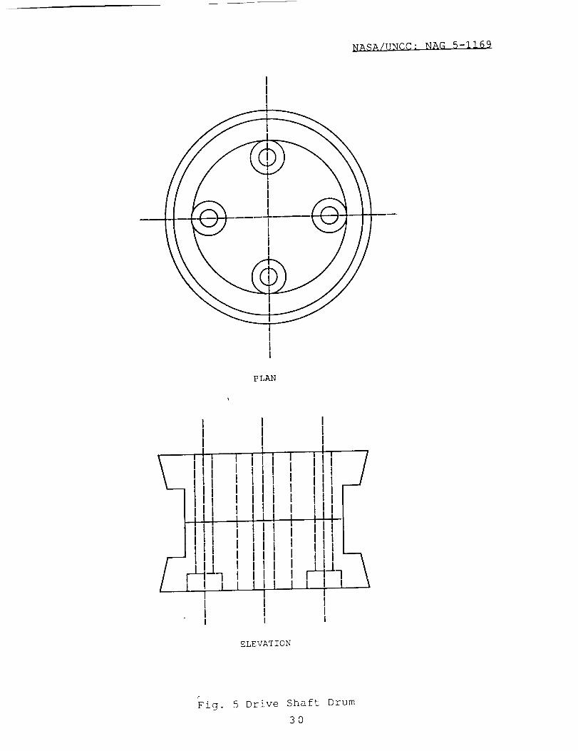
NASA/UNCC: NAG 5-1169
P LAN
I I
kiI
I!'
I
/--,, ]
IIII
ELEVATION
Fig. 5 Drive Shaft Drum
30
NASA/UNCC: NAG 5-1169
Striker
Cam
Lifting Magnet
Coils
Fig. 6 Drive Drum
31

NASA/UNCC: NAG 5-1169
DRIVE ROD COIL
DRIVE RING OSCILLATING MOTION
CONTRACTING
MAGNETOSTRICTIVE
RODDRIVE SHAFT DRUM
---4&--
k
CW
DRIVE DRUM
EXPANDING
MAGNETOSTRICTIVE
ROD
DRIVE CAM
COUNTERCLOCKWISE ROLLERS
ARE MAGNETICALLY LIFTED
G: OUTPUT FORCE
FIG. 7 FUNCTIONAL OPERATION OF DRIVE
32

NASA/UNCC: NAG 5-1169
FNPL FFPL _
FPL
EFB
FIG. 8 (a) PRELOAD FORCES
33
NASA/UNCC: NAG 5-1169
PRELOAD
DRIVE R E CONE DRIVE SHAFT
NORMAL
FORCES
SF = 0Z
a. Preload Forces on Drive Cones
q
DRIVE RING DRIVE CC
PRELOAD
_E
DRIVE SHAFT
TION
SFZ
b. Forces on Drive Cones Under Load
= 0
FIG. 8 (b) PRELOAD FORCES
34

NASA/UNCC: NAG 5-1169
Spring Com_
Region
Preload
(0.001 in each side)
l[
I
iI
Flat Cut in
Bearing Material
Tool Steel
Guide Rod
Guide Spring/Bearing
Preload
(0.001 in each side)
Fig. 9 Guide Spring
35

NASA/UNCC: NAG 5-I16_
2OO
Backlash
;and/
Dead Zone
Output Stroke at 60 Ft
Lbs
I00
to
U
0
0.5
Drive Displacement
g
(Hysteresis)
(a}
LEGEND
Roller in Drive Cam
Roller on Drive Shaft Drum
CONTACT STRESSES
Fig. i0 Regions of Backlash, Dead Zones and Hysteresis
36

NASA/UNCC: NAG 5-1169
Backlash and
Dead Zone /Output Stroke at 60 Ft Lbs
O
O
o
(D£]
6O
2C
0.5 1
Walking (Hysteresis)
LEGEND
Drive cam
Drive Roller
Drive Drum
(b)
DEFORMATIONS
Fig. i0 Regions of Backlash, Dead Zones and Hysteresis
37

NASA/UNCC: NAG 5-1169
A
O
O
9O
6_
3_
Backlash and
Dead ZoneUseful Stroke
J-"7
0.5
Drive Displacement
(c)
Steady State Torque Output
Fig. i0 Regions of Backlash, Dead Zones and Hysteresis
38

NASA/UNCC: NAG 5-1169
Highest pet" for-
mance material
TD ,Dy :Fe, 43
d,recttonally
solidified
(FSZM) near
single crystal -
6.3ram (.25 in.)
diameter
PRESTRESS
r._ 2.0 KSI
• 1.8 KSI
• 0.0 KSI
ETREMATERFENOL-DMAGNETOSTRICTiON
Free Stand Zone Melt (FSZM)
2000.
1500.
o
1OOO.
500.
O.
- 3000. -2000. -1OO0. O. 1000. 2000.
Applied Field, H(Oersted)
f
3uO0.
_:_.;.;> :£,:..:<q ,,_
Typical per-
formance of
Tb 3Dy.TFe, 93
directionally
solidified (M8)
material- lOmm
(.4 in.) diameter
PRESTRESS
• 2.0 KSI
• 1.0 KSI
• 0.0 KSl
2000.
Q.t_
15OO.
L
o 1000.
t_
500.
Modified Bridgman (MB)
"1JrO.
- 3000 - 2000 - 1000. O. 1000 2000. 3UO0.
Applied Field, H (Oersted)
Fig. 11 Performance Characteristics of FSZM Terfenol Rods
39

/
J(Q) TIME
NASAIUNCC :
TYPE OF LU8R_C_NT
1. UNuJSAIC_.£EO
2 BOUND&I_Y LUSRICATCO
3 FLUIO FiLM LUBRIC_T_O
FIXED CONDITIONS
MATERIAL
LUBRICANT
VISCOSITY
GEOMETRY
FINISH
LUBRICANT QUANTITY
AMBIENT T E MPE R,_T UI_E
4MBIENT /_TMOSPHERE
NAG 5-1169
Fig. 12
(b) LOAD
LJ
Q:
'22
tlJ
#d) TEMPERATURE
(c) VELOCITY
l-
rr
rr
e) FILM THICKNESS
Effect
W2
i,,
Wl
>
rr
, ,/RUN IN I ItI I
.... I__
II
r I I! Itl t2
of Operational
TIME ----"
5
3Variables on Wea_
->
-7
4 0 :
)
Rate

PRELIMINARYDRAWINGS
OF
MAGNETOSTRICTIVEDIRECT DRIVE MOTOR

NASA/UNCC: NAG 5-1169
-.. ]-_() . .
IIIIIIII
i IIII
F_ 3/8"318Tj!
Yl
1/4 ' '
1/16' ' through
DRIVE ROLLER
MATERIAL: SAE 52100
NOS: 32
DRIVE ROLLER
DESIGNED BY: JMV DRAWNED BY" DPN
SR. NO. 1
DATE: 8/8/90
SCALE : i : I
41

4 M6*I SOCKET HEAD
CAP SCREWS
NASA/UNCC: NAG 5-1169I
l
3/4' ' 6- SPLINE
\,, "-... ,._y., _/ t/
IPLaN
II
I I_ 2 i_I16" ..Jl
It', t "nlII I 2 1116" _I
iI " i "7I I--'! : , :iI , I
, J[i_Ni_ , ,
il I '/ i_/i!l I !I I
_,,_,,HI:,, i:ir L_*_VI'!: :',_-_: -.... I #. i _
' i
ELEVATION
318 ' '
t 3/8 ' '
DRIVE SHAFT DRUM
MATERIAL: SAE 52100
NOS: ]
DRIVE SHAFT DRUM SR. NO. 2
DESIGNED BY: JMV DRAWLED BY: DPN DATE: 8/8/90
SCALE : i :i_U ---_--
42

NASA/UNCC: NAG 5-1169
18, I/4' ' DIA
THROUGH HOLES
ON 3 !/16'' PCD
PLAN
DRIVE DRUM
MATERIAL: SAE 52100
NOS: 1
DESIGNED BY:
DRIVE DRUM
JMV DRAWNED BY: DPN
SR. NO. 3
DATE: 8/8/90
SCALE : 1 :1
43

I/8" , .
I I
11141
3-21/32"
'' DIA
HOLES
IlqI
NASA/UNCC: NAG 5-1169
I
II
4-7/16"
!
4-3/!6"
I
3-11/16"
|
3-I/16"
2-37/64"
!
3-7/16"
!
I
I
4-11/16"
iiiI
r I iI_ -
ELEVATICN
I II I
1/8''
Yl!
DRIVE DRUM
MATERIAL: SAE 52100
NOS: 1
DESIGNED BY:
DRIVE DRUM
JMV DRAWNED BY : DPN
SR. NO. 3
DATE: 8/8/90
SCALE : I :I
44

NASA/UNCC: NAG 5-1169
i/4'' DIA, 1/4''DEEP
TAPPED HOLE
I/4''
i 1/2''
!..............t
1 2 vl
.<_C--
=
P LA N
----J._--- i-i/4"e
-_ 1-5/8" r
TORQUE ARM PLATE
DESIGNED BY: JMV DRAWNED BY: DPN
SR. NO. 4
DATE: 8/8/90
SCALE : I :I
45

I4) 3/8''_
• o
I !
I I
I I(_ I/2" _ . .
¢ 5/8,
I
I
I
4:) 1/2'' "_ !!'iI
I
I i
I
4) 3/5' ', 6-SPLINE _ I
_) 1/2 ' '
4) 5/,8,'
_ -_,
4) 3/8' ' _
1/8"'45 CHAMFERj
BOTH ENDS
,--_-----
1-1/16"
__!___ili
NASA/UNCC: NAG 5-1169
..... F---7
I
iiI
I
I
I
I
I
I
I
i
_ [ ............ l"_ ..... -t- 2-1
....:,____:
2-1/2"
6-3/8"
t2,,
L .... 2'
SHAFT
MATERIAL: SAE 52100
N_. i
DESIGNED BY:
DRIVE SHAFT
JMV DRAWNED BY: DPN
SR. NO. 5
DATE: 8/8/90
SCALE : 1 : 1
46

NASA/UNCC: NAG 5-1169
O
iiI
I
II
ii
I
I
IiIII
I
18, 1/8' ' DIA EQUISPACED
HOLES ON 3 1/16'' PCD
PLAN
STRIKER PLATE
DESIGNED BY: JMV DRAWNED BY: DPN
SR. NO. 6
DATE: 8/8/90
SCALE: i:i {} ---<+--
47

NASA/UNCC: NAG 5-1169
I
lit
l
i
2 13/16"
2 15/16"
!
N I;k\\\\"I1'.III
I
4 3/16"w
I/8''
° '_"
ELEVATION
STRIKER PLATE
MATERIAL: SS 316
NOS: 2
STRIKER PLATE
DESIGNED BY: JMV DRAWNED BY: DPN
SR. NO. 6
DATE: 8/8/90
SCALE : 1 :1 ,,;,,-.,,_.g ---_}--
48

NASA/UNCC: NAG 5-1169
I k., 3/8 ' 'I Ii I_ 11/16''
II
PLAN !
II I ,
IIi lla,,
i
i l_I, ,i,iI
__.....!/._"..__.
ELEVATION
STRIKER DETAILS
MATERIAL: SS 3!6
STRIKER DETAILS SR. NO. 6
DESIGNED BY: JMV DRAWNED BY: DPN DATE: 8/8/90
SCALE : 1 :1
I
49

I
CASING
MATERIAL: ALUMINUM 2014-T6
NOS: 1
I
iI I |I
[ .... --F-
I
iI
I
1
I
75
TAPPED HOLE
4 15/!6''
..... _ o
A
DESIGNED
CASING
BY: JMV DRAWNED BY: DPN
SR. NO. 7
DATE: 8/8/90
SCALE • 1 : 1
5O

1-7/16"
I2-13/16" . _ .....
\
\
\
\
<\
\\
\
\
.!\\\\\\\\\\\\ I
II
Il-lTM
I '
i-"
NASA/UNCC: NAG 5-1169
I4-7/16"
I
4-11/16"
I
4-15/16"
I
I
I
ELEVATION
CASING
MATERIAL: ALUMINUM 2014-T6
NOS: 1
4-1 '4"
DESIGNED BY :
CASING
JMV DRAWNED BY : DPN
SR. NO. 7
DATE: 8/8/90
SCALE : i :I --
51

NASA/UNCC: NAG 5-1169
(_) 4 11/16"
A
6, (_)4 i/4"
TAPPED EQUISP_
HOLES ON 3 13,
A
P LA N
END
DESIGNED BY" JMV
COVERS
DRAWNED BY: DPN
SR.
DATE :
NO. 8
818190
SCALE" 1 :1
52

NASA/UNCC: NAG 5-1169
1/16' '
\CED
'I 6" PCD
I
I
i I I
! --l_ • Ii !_, I I
I l I _i_ii II IiI'_ lI I I Ii _ _-S.132"---_ II I I
1-9/16"
4-61/64" w'--I
SECTION A-A
3/16''
3/8''
.!__
ELEVATION
END COVER
MATERIAL: ALUMINIUM
2014-T6
NOS: 2
DESIGNED BY:
END COVERS
JMV DRAWNED BY: DPN
SR. NO. 8
DATE: 8/8/90
SCALE • i :iL 5/#A ....
53

NASA/UNCC: NAG 5-1169
' BOTH iNDS
.....k!.......I
' 1iii
!
iiIIi
P l[h N
iIIII
i/4''
, [!
i "_-_" _
!
TERFENOL D
TERFENOL RODS
DESIGNED BY: JMV DRAWNED BY: DPN
SR. NO. 9
DATE: 8/8/90
SCALE : I "I _ _,-____.
54

G
B
\\\/\1\/
\11N\\\\\
\\\
\\\\\\\\\\\,,_
N\\m
,..N_ASA/UNCC :
\\
\\
\\
®
//
/(--12)
• |
ELEVATION
NAG 5-1169
p\\\
/\
\_\
\\
\\X\,'x\\\
\\\\\\
G
A
\\
/\ \
N
/\ \
©MAGNETO$TRICTIVE DIRECT DRIVE MOTOR (i)
DESIGNED BY- JMV DRAWNED BY: DPN DATE: 8/8/90
SCALE : 1 :1 /,_ __<}--.
55

NASA/UNCC: NAG 5-1169
PLAN
MAGNETO$TRICT!VE DIRECT DRIVE MOTOR (2)
DESIGNED BY: _,_ DRAWNED BY: DPN DATE: 8/8/90
SCALE: I:i _j_ -- -_--.
56

NASA/UNCC: NAG 5-1169
I
I \I
I I/
PLAN
SECTION A-A
MAGNETQSTRICTIVE DIRECT DRIVE MOTOR (3)
DESIGNED BY: JMV DRAWNED BY: DPN DATE: 8/8/90
SCALE: i:i
57

NASA/UNCC: NAG 5-1169
PLAN
SECTION B-B
MAGNETQ$TRICTIVE DIRECT DRIVE MQTQR (4)
DESIGNED BY: jMV DRAWNED BY: DPN DATE: 8/8/90
SCALE: I:I --58

NASA/UNCC: NAG 5-1169
tA
Ii .....
I
I
A
PLAN
SECTION C-C
MA_NETOSTRICTIVE DIRECT DRIVE MQTOR (5)
DESIGNED BY: JMV DRAWNED BY: DPN DATE: 8/8/90
SCALE: i:i _h __<__-.'¢.J
59
NASA/UNCC: NAG 5-1169
12 BEARINGS FAG 6001 2RSR 2
I! ELECTROMAGNETIC COIL COPPER AWG 23 8
I0 DRIVE COILS COPPER AWG 23 8
9 TERFENOL RODS TERFENOL D 8
ALUMINUM
8 END COVERS 2014-T6 2
ALUMINUM
7 CASING 2014-T6 1
6 STRIKER PLATE SS 316 2
5 SHAFT SS 316 1
4 TORQUE ARM PLATE SS 316 8
3 DRIVE DRUM SAE 52100 1
2 DRIVE SHAFT DRUM SAE 52100 1
1 DRIVE CONE SAE 52100 36
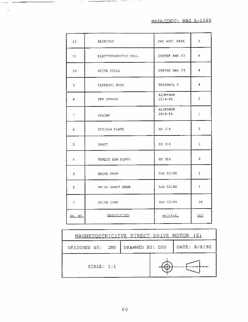
DESCRIPTION MATERIAL NOS
MAGNETQSTRICTIVE DIRECT DRIVE MQTQR (6)
DESIGNED BY: JMV DRAWNED BY: DPN DATE: 8/8/90
SCALE : 1 :1
I
i
6O

NASA/UNCC: NAG 5-1169
.
°
°
References
Engineering Electromagnetics by William H. Hyat, McGraw-
Hill Book Company, Fifth Edition, pp. 298, (1989).
Application Manual For The Design of Terfenol-D
Magnetostrictive Transducers, Prepared for EdgeTechnologies, Inc., by Dr. John L. Butler
Fein, R.S. : "Equations For The Calculation of The
Antiwear Number," Contribution to the Wear ControlHandbook by Texaco Inc.
61