Magnetospheric Accretion in Classical T Tauri Stars

J. Bouvier, S. H. P. AlencarLaboratoire d’Astrophysique Grenoble

T. J. HarriesUniversity of Exeter

C. M. Johns-KrullRice University

M. M. RomanovaCornell University

The inner 0.1 AU around accreting T Tauri stars hold clues to many physical processesthat characterize the early evolution of solar-type stars.The accretion-ejection connectiontakes place at least in part in this compact magnetized region around the central star, withthe inner disk edge interacting with the star’s magnetosphere thus leading simultaneously tomagnetically channeled accretion flows and to high velocitywinds and outflows. The magneticstar-disk interaction is thought to have strong implications for the angular momentum evolutionof the central system, the inner structure of the disk, and possibly for halting the migration ofyoung planets close to the stellar surface. We review here the current status of magnetic fieldmeasurements in T Tauri stars, the recent modeling efforts of the magnetospheric accretionprocess, including both radiative transfer and multi-D numerical simulations, and summarizecurrent evidence supporting the concept of magnetically-channeled accretion in young stars.We also discuss the limits of the models and highlight observational results which suggest thatthe star-disk interaction is a highly dynamical and time variable process in young stars.

1. THE MAGNETIC ACCRETION PARADIGM

T Tauri stars are low-mass stars with an age of a fewmillion years, still contracting down their Hayashi tracksto-wards the main sequence. Many of them, the so-called clas-sical T Tauri stars (CTTSs), show signs of accretion from acircumstellar disk (see, e.g.,Menard and Bertout, 1999 fora review). Understanding the accretion process in T Tauristars is one of the major challenges in the study of pre-mainsequence evolution. Indeed, accretion has a significant andlong lasting impact on the evolution of low mass stars byproviding both mass and angular momentum. The evolutionand ultimate fate of circumstellar accretion disks have alsobecome increasingly important issues since the discoveryof extrasolar planets and planetary systems with unexpectedproperties. Deriving the properties of young stellar systems,of their associated disks and outflows is therefore an impor-tant step towards the establishment of plausible scenariosfor star and planet formation.

The general paradigm of magnetically controlled accre-tion onto a compact object is used to explain many of themost fascinating objects in the Universe. This model is aseminal feature of low mass star formation, but it is also en-countered in theories explaining accretion onto white dwarfstars (the AM Her stars, e.g.,Warner, 2004), accretion

onto pulsars (the pulsating X-ray sources , e.g.,Ghosh andLamb, 1979a), and accretion onto black holes at the cen-ter of AGNs and microquasars (Koide et al., 1999). Strongsurface magnetic fields have long been suspected to existin TTSs based on their powerful X-ray and centrimetric ra-dio emissions (Montmerle et al., 1983;Andre, 1987). Sur-face fields of order of 1-3 kG have recently been derivedfrom Zeeman broadening measurements of CTTS photo-spheric lines (Johns Krull et al., 1999a, 2001;Guentheret al., 1999) and from the detection of electron cyclotronmaser emission (Smith et al., 2003). These strong stellarmagnetic fields are believed to significantly alter the accre-tion flow in the circumstellar disk close to the central star.

Based on models originally developed for magnetizedcompact objects in X-ray pulsars (Ghosh and Lamb, 1979a)and assumingthat T Tauri magnetospheres are predomi-nantly dipolar on the large scale,Camenzind(1990) andKonigl (1991) showed that the inner accretion disk is ex-pected to be truncated by the magnetosphere at a distanceof a few stellar radii above the stellar surface for typicalmass accretion rates of 10−9 to 10−7 M yr−1 in the disk(Basri and Bertout, 1989;Hartigan et al., 1995;Gullbringet al., 1998). Disk material is then channeled from the diskinner edge onto the star along the magnetic field lines, thusgiving rise to magnetospheric accretion columns. As the

1

free falling material in the funnel flow eventually hits thestellar surface, accretion shocks develop near the magneticpoles. The basic concept of magnetospheric accretion in TTauri stars is illustrated in Figure 1.

The successes and limits of current magnetospheric ac-cretion models in accounting for the observed properties ofclassical T Tauri systems are reviewed in the next sections.Sect. 2 summarizes the current status of magnetic field mea-surements in young stars, Sect. 3 provides an account ofcurrent radiative transfer models developed to reproduce theobserved line profiles thought to form at least in part in ac-cretion funnel flows, Sect. 4 reviews current observationalevidence for a highly dynamical magnetospheric accretionprocess in CTTSs, and Sect. 5 describes the most recent 2Dand 3D numerical simulations of time dependent star-diskmagnetic interaction.

Fig. 1.— A sketch of the basic concept of magnetosphericaccretion in T Tauri stars (fromCamenzind, 1990).

2. MAGNETIC FIELD MEASUREMENTS

2.1. Theoretical Expectations for T Tauri MagneticFields

While the interaction of a stellar magnetic field with anaccretion disk is potentially very complicated (e.g.,Ghoshand Lamb, 1979a,b), we present here some results from theleading treatments applied to young stars.

The theoretical idea behind magnetospheric accretion isthat the ram pressure of the accreting material (Pram =0.5ρv2) will at some point be offset by the magnetic pres-sure (PB = B2/8π) for a sufficiently strong stellar field.Where these two pressures are equal, if the accreting ma-terial is sufficiently ionized, its motion will start to be con-trolled by the stellar field. This point is usually referred toas the truncation radius (RT ). If we consider the case ofspherical accretion, the ram pressure becomes

Pram =1

2ρv2 =

Mv

2r2. (2.1)

If we then assume a dipolar stellar magnetic field whereB = B∗(R∗/r)3 and set the velocity of the accreting ma-terial equal to the free-fall speed, the radius at which themagnetic field pressure balances the ram pressure of the ac-creting material is

RT

R∗

=B

4/7

∗ R5/7

∗

M2/7(2GM∗)1/7= 7.1B

4/7

3M

−2/7

−8M

−1/7

0.5 R5/7

2,

(2.2)whereB3 is the stellar field strength in kG,M−8 is the massaccretion rate in units of10−8 M yr−1, M0.5 is the stellarmass in units of 0.5 M, andR2 is the stellar radius in unitsof 2 R. Then, forB∗ = 1 kG and typical CTTS properties(M∗ = 0.5 M, R∗ = 2 R, andM = 10−8 M yr−1),the truncation radius is about 7 stellar radii.

In the case of disk accretion, the coefficient above ischanged, but the scaling with the stellar and accretion pa-rameters remains the same. In accretion disks around youngstars, the radial motion due to accretion is relatively lowwhile the Keplerian velocity due to the orbital motion isonly a factor of21/2 lower than the free-fall velocity. Thelow radial velocity of the disk means that the disk densitiesare much higher than in the spherical case, so that the diskram pressure is higher than the ram pressure due to spheri-cal free-fall accretion. As a result, the truncation radiuswillmove closer to the star. In this regard, equation 2.2 givesan upper limit for the truncation radius. As we will dis-cuss below, this may be problematic when we consider thecurrent observations of stellar magnetic fields. In the caseof disk accretion, another important point in the disk is thecorotation radius,RCO, where the Keplerian angular veloc-ity is equal to the stellar angular velocity. Stellar field lineswhich couple to the disk outside ofRCO will act to slowthe rotation of the star down, while field lines which coupleto the disk insideRCO will act to spin the star up. Thus,the value ofRT relative toRCO is an important quantityin determining whether the star speeds up or slows downits rotation. For accretion onto the star to proceed, we havethe relationRT < RCO. This follows from the idea that atthe truncation radius and interior to that, the disk materialwill be locked to the stellar field lines and will move at thesame angular velocity as the star. OutsideRCO the stellarangular velocity is greater than the Keplerian velocity, sothat any material there which becomes locked to the stellarfield will experience a centrifugal force that tries to fling thematerial away from the star. Only insideRCO will the netforce allow the material to accrete onto the star.

Traditional magnetospheric accretion theories as appliedto stars (young stellar objects, white dwarfs, and pulsars)suggest that the rotation rate of the central star will be setby the Keplerian rotation rate in the disk near the pointwhere the disk is truncated by the stellar magnetic fieldwhen the system is in equilibrium. Hence these theoriesare often referred to as disk locking theories. For CTTSs,we have a unique opportunity to test these theories sinceall the variables of the problem (stellar mass, radius, rota-tion rate, magnetic field, and disk accretion rate) are mea-

2

sureable in principle (seeJohns–Krull and Gafford, 2002).Under the assumption that an equilibrium situation exists,Konigl (1991),Cameron and Campbell(1993), andShu etal. (1994) have all analytically examined the interactionbetween a dipolar stellar magnetic field (aligned with thestellar rotation axis) and the surrounding accretion disk.Asdetailed inJohns–Krull et al.(1999b), one can solve for thesurface magnetic field strength on a CTTS implied by eachof these theories given the stellar mass, radius, rotation pe-riod, and accretion rate. For the work ofKonigl (1991), theresulting equation is:

B∗ = 3.43( ε

0.35

)7/6( β

0.5

)−7/4( M∗

M

)5/6

×

×( M

10−7 M yr−1

)1/2( R∗

R

)−3( P∗

1 dy

)7/6

kG, (2.3)

In the work ofCameron and Campbell(1993) the equationfor the stellar field is:

B∗ = 1.10γ−1/3

( M∗

M

)2/3( M

10−7 M yr−1

)23/40

×

×( R∗

R

)−3( P∗

1 dy

)29/24

kG, (2.4)

Finally, fromShu et al.(1994), the resulting equation is:

B∗ = 3.38( αx

0.923

)−7/4( M∗

M

)5/6( M

10−7 M yr−1

)1/2

×

×( R∗

R

)−3( P∗

1 dy

)7/6

kG, (2.5)

All these equations contain uncertain scaling parameters(ε, β, γ, αx) which characterize the efficiency with whichthe stellar field couples to the disk or the level of verticalshear in the disk. Each study presents a best estimate forthese parameters allowing the stellar field to be estimated(Table 1). Observations of magnetic fields on CTTSs canthen serve as a test of these models.

To predict magnetic field strengths for specific CTTSs,we need observational estimates for certain system param-eters. We adopt rotation periods fromBouvier et al.(1993,1995) and stellar masses, radii, and mass accretion ratesfrom Gullbring et al. (1998). Predictions for each analyticstudy are presented in Table 1. Note, these field strengthsare the equatorial values. The field at the pole will be twicethese values and the average over the star will depend onthe exact inclination of the dipole to the observer, but fori = 45 the average field strength on the star is∼ 1.4 timesthe values given in the Table. Because of differences inunderlying assumptions, these predictions are not identical,but they do have the same general dependence on systemcharacteristics. Consequently, field strengths predictedbythe 3 theories, while different in scale, nonetheless have thesame pattern from star to star. Relatively weak fields arepredicted for some stars (DN Tau, IP Tau), but detectablystrong fields are expected on stars such as BP Tau.

2.2. Measurement Techniques

Virtually all measurements of stellar magnetic fieldsmake use of the Zeeman effect. Typically, one of two gen-eral aspects of the Zeeman effect is utilized: (1) Zeemanbroadening of magnetically sensitive lines observed in in-tensity spectra, or (2) circular polarization of magneticallysensitive lines. Due to the nature of the Zeeman effect, thesplitting due to a magnetic field is proportional toλ2 of thetransition. Compared with theλ1 dependence of Dopplerline broadening mechanisms, this means that observationsin the infrared (IR) are generally more sensitive to the pres-ence of magnetic fields than optical observations.

The simplest model of the spectrum from a magnetic starassumes that the observed line profile can be expressed asF (λ) = FB(λ) ∗ f + FQ(λ) ∗ (1 − f); whereFB is thespectrum formed in magnetic regions,FQ is the spectrumformed in non-magnetic (quiet) regions, andf is the fluxweighted surface filling factor of magnetic regions. Themagnetic spectrum,FB, differs from the spectrum in thequiet region not only due to Zeeman broadening of the line,but also because magnetic fields affect atmospheric struc-ture, causing changes in both line strength and continuumintensity at the surface. Most studiesassumethat the mag-netic atmosphere is in fact the same as the quiet atmospherebecause there is no theory to predict the structure of themagnetic atmosphere. If the stellar magnetic field is verystrong, the splitting of theσ components is a substantialfraction of the line width, and it is easy to see theσ compo-nents sticking out on either side of a magnetically sensitiveline. In this case, it is relatively straightforward to measurethe magnetic field strength,B. Differences in the atmo-spheres of the magnetic and quiet regions primarily affectthe value off . If the splitting is a small fraction of the in-trinsic line width, then the resulting observed profile is onlysubtly different from the profile produced by a star with nomagnetic field and more complicated modelling is requiredto be sure all possible non-magnetic sources (e.g., rotationand pressure broadening) have been properly constrained.

In cases where the Zeeman broadening is too subtle todetect directly, it is still possible to diagnose the presence ofmagnetic fields through their effect on the equivalent widthof magnetically sensitive lines. For strong lines, the Zee-man effect moves theσ components out of the partially sat-urated core into the line wings where they can effectivelyadd opacity to the line and increase the equivalent width.The exact amount of equivalent width increase is a compli-cated function of the line strength and Zeeman splitting pat-tern (Basri et al., 1992). This method is primarily sensitiveto the product ofB multiplied by the filling factorf (Basriet al., 1992,Guenther et al., 1999). Since this method re-lies on relatively small changes in the line equivalent width,it is very important to be sure other atmospheric parameterswhich affect equivalent width (particularly temperature)areaccurately measured.

Measuring circular polarization in magnetically sensitivelines is perhaps the most direct means of detecting magnetic

3

TABLE 1

PREDICTED MAGNETIC FIELD STRENGTHS

M∗ R∗ M × 108 Prot Ba∗ Bb

∗ Bc∗ RCO Bobs

Star (M) (R) (Myr−1) (days) (G) (G) (G) (R∗) (kG)

AA Tau 0.53 1.74 0.33 8.20 810 240 960 8.0 2.57BP Tau 0.49 1.99 2.88 7.60 1370 490 1620 6.4 2.17CY Tau 0.42 1.63 0.75 7.90 1170 390 1380 7.7DE Tau 0.26 2.45 2.64 7.60 420 164 490 4.2 1.35DF Tau 0.27 3.37 17.7 8.50 490 220 570 3.4 2.98DK Tau 0.43 2.49 3.79 8.40 810 300 950 5.3 2.58DN Tau 0.38 2.09 0.35 6.00 250 80 300 4.8 2.14GG Tau A 0.44 2.31 1.75 10.30 890 320 1050 6.6 1.57GI Tau 0.67 1.74 0.96 7.20 1450 450 1700 7.9 2.69GK Tau 0.46 2.15 0.64 4.65 270 90 320 4.2 2.13GM Aur 0.52 1.78 0.96 12.00 1990 660 2340 10.0IP Tau 0.52 1.44 0.08 3.25 240 60 280 5.2TW Hya 0.70 1.00 0.20 2.20 900 240 1060 6.3 2.61T Tau 2.11 3.31 4.40 2.80 390 110 460 3.2 2.39

NOTE.—Magnetic field values come from applying the theory of (a) Konigl (1991), (b) Cameron andCampbell, or (c) Shu et al. (1994). These are the equatorial field strengths assuming a dipole magneticfield.

fields on stellar surfaces, but is also subject to several limi-tations. When viewed along the axis of a magnetic field, theZeemanσ components are circularly polarized, but with op-posite helicity; and theπ component is absent. The helicityof theσ components reverses as the polarity of the field re-verses. Thus, on a star like the Sun that typically displaysequal amounts of+ and− polarity fields on its surface, thenet polarization is very small. If one magnetic polarity doesdominate the visible surface of the star, net circular polar-ization is present in Zeeman sensitive lines, resulting in awavelength shift between the line observed through right-and left-circular polarizers. The magnitude of the shift rep-resents the surface averaged line of sight component of themagnetic field (which on the Sun is typically less than 4 Geven though individual magnetic elements on the solar sur-face range from∼ 1.5 kG in plages to∼ 3.0 kG in spots).Several polarimetric studies of cool stars have generallyfailed to detect circular polarization, placing limits on thedisk-averaged magnetic field strength present of10 − 100G (e.g.,Vogt, 1980;Brown and Landstreet, 1981;Borra etal., 1984). One notable exception is the detection of circu-lar polarization in segments of the line profile observed onrapidly rotating dwarfs and RS CVn stars where Dopplerbroadening of the line “resolves” several independent stripson the stellar surface (e.g.,Donati et al., 1997;Petit et al.,2004;Jardine et al., 2002).

2.3. Mean Magnetic Field Strength

TTS typically havev sin i values of 10 km s−1, whichmeans that observations in the optical typically cannot de-tect the actual Zeeman broadening of magnetically sensitivelines because the rotational broadening is too strong. Never-theless, optical observations can be used with the equivalentwidth technique to detect stellar fields.Basri et al. (1992)were the first to detect a magnetic field on the surface of aTTS, inferring a value ofBf = 1.0 kG on the NTTS Tap35. For the NTTS Tap 10,Basri et al. (1992) find only anupper limit ofBf < 0.7 kG. Guenther et al.(1999) applythe same technique to spectra of 5 TTSs, claiming signif-icant field detections on two stars; however, these authorsanalyze their data using models off by several hundred Kfrom the expected effective temperature of their target stars,always a concern when relying on equivalent widths.

As we saw above, observations in the IR will help solvethe difficulty in detecting direct Zeeman broadening. Forthis reason and given the temperature of most TTSs (K7 -M2), Zeeman broadening measurements for these stars arebest done using several TiI lines found in the K band. Ro-bust Zeeman broadening measurements require Zeeman in-sensitive lines to constrain nonmagnetic broadening mech-anisms. Numerous CO lines at 2.31µm have negligibleLande-g factors, making them an ideal null reference.

It has now been shown that the Zeeman insensitive COlines are well fitted by models with the same level of rota-tional broadening as that determined from optical line pro-

4

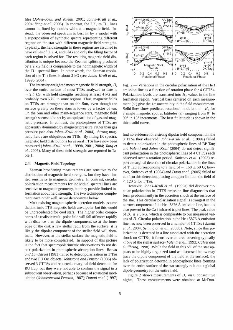
files (Johns–Krull and Valenti, 2001; Johns–Krull et al.,2004;Yang et al., 2005). In contrast, the 2.2µm Ti I linescannot be fitted by models without a magnetic field. In-stead, the observed spectrum is best fit by a model witha superposition of synthetic spectra representing differentregions on the star with different magnetic field strengths.Typically, the field strengths in these regions are assumed tohave values of 0, 2, 4, and 6 kG and only the filling factor ofeach region is solved for. The resulting magnetic field dis-tribution is unique because the Zeeman splitting producedby a 2 kG field is comparable to the nonmagnetic width ofthe Ti I spectral lines. In other words, the Zeeman resolu-tion of the Ti I lines is about 2 kG (seeJohns–Krull et al.,1999b, 2004).

The intensity-weighted mean magnetic field strength,B,over the entire surface of most TTSs analyzed to date is∼ 2.5 kG, with field strengths reaching at least 4 kG andprobably even 6 kG in some regions. Thus, magnetic fieldson TTSs are stronger than on the Sun, even though thesurface gravity on these stars is lower by a factor of ten.On the Sun and other main-sequence stars, magnetic fieldstrength seems to be set by an equipartition of gas and mag-netic pressure. In contrast, the photospheres of TTSs areapparently dominated by magnetic pressure, rather than gaspressure (see alsoJohns–Krull et al., 2004). Strong mag-netic fields are ubiquitous on TTSs. By fitting IR spectra,magnetic field distributions for several TTSs have now beenmeasured (Johns–Krull et al., 1999b, 2001, 2004;Yang etal., 2005). Many of these field strengths are reported in Ta-ble 1.

2.4. Magnetic Field Topology

Zeeman broadening measurements are sensitive to thedistribution of magnetic field strengths, but they have lim-ited sensitivity to magnetic geometry. In contrast, circularpolarization measurements for individual spectral lines aresensitive to magnetic geometry, but they provide limited in-formation about field strength. The two techniques comple-ment each other well, as we demonstrate below.

Most existing magnetospheric accretion models assumethat intrinsic TTS magnetic fields are dipolar, but this wouldbe unprecedented for cool stars. The higher order compo-nents of a realistic multi-polar field will fall off more rapidlywith distance than the dipole component, so at the inneredge of the disk a few stellar radii from the surface, it islikely the dipolar component of the stellar field will dom-inate. However, at the stellar surface the magnetic field islikely to be more complicated. In support of this pictureis the fact that spectropolarimetric observations do not de-tect polarization in photospheric absorption lines:Brownand Landstreet(1981) failed to detect polarization in T Tauand two FU Ori objects;Johnstone and Penston(1986) ob-served 3 CTTSs and reported a marginal field detection forRU Lup, but they were not able to confirm the signal in asubsequent observation, perhaps because of rotational mod-ulation (Johnstone and Penston, 1987);Donati et al.(1997)

−4

−2

0

2

4

BZ (

kG)

i=66B=−4.0 kG

χ2=20χ2=2.1φ=12

AA Tau

i=38B=2.1 kG

χ2=65χ2=3.7φ=48

BP Tau

0 0.2 0.4 0.6 0.8 1 Rotational Phase

−4

−2

0

2

4

BZ (

kG)

i=74B=−2.3 kG

χ2=57χ2=0.9φ=10

DF Tau

Magnetic SpotModels

0 0.2 0.4 0.6 0.8 1 Rotational Phase

i=44B=2.7 kG

χ2=20χ2=4.9φ=60

DK Tau

Fig. 2.— Variations in the circular polarization of the HeI

emission line as a function of rotation phase for 4 CTTSs.Polarization levels are translated intoBz values in the lineformation region. Vertical bars centered on each measure-ment (×) give the 1σ uncertainty in the field measurement.Solid lines show predicted rotational modulation inBz fora single magnetic spot at latitudes (φ) ranging from 0 to90 in 15 increments. The best fit latitude is shown in thethick solid curve.

find no evidence for a strong dipolar field component in the3 TTSs they observed;Johns–Krull et al. (1999a) failedto detect polarization in the photospheric lines of BP Tau;andValenti and Johns–Krull(2004) do not detect signifi-cant polarization in the photospheric lines of 4 CTTSs eachobserved over a rotation period.Smirnov et al.(2003) re-port a marginal detection of circular polarization in the linesof T Tau corresponding to a field of∼ 150 ± 50 G; how-ever,Smirnov et al.(2004) andDaou et al.(2005) failed toconfirm this detection, placing an upper limit on the field of≤ 120 G for T Tau.

However,Johns–Krull et al. (1999a) did discover cir-cular polarization in CTTS emission line diagnostics thatform predominantly in the accretion shock at the surface ofthe star. This circular polarization signal is strongest inthenarrow component of the HeI 5876A emission line, but it isalso present in the CaI infrared triplet lines. The peak valueof Bz is 2.5 kG, which is comparable to our measured val-ues ofB. Circular polarization in the HeI 5876A emissionline has now been observed in a number of CTTSs (Valentiet al., 2004;Symington et al., 2005b). Note, since this po-larization is detected in a line associated with the accretionshock on CTTSs, it forms over an area covering typically< 5% of the stellar surface (Valenti et al., 1993;Calvet andGullbring, 1998). While the field in this 5% of the star ap-pears to be highly organized (and as discussed below maytrace the dipole component of the field at the surface), thelack of polarization detected in photospheric lines formingover the entire surface of the star strongly rule out a globaldipole geometry for the entire field.

Figure 2 shows measurements ofBz on 6 consecutivenights. These measurements were obtained at McDon-

5

ald Observatory, using the Zeeman analyzer described byJohns–Krull et al. (1999a). The measured values ofBz

vary smoothly on rotational timescales, suggesting that uni-formly oriented magnetic field lines in accretion regionssweep out a cone in the sky, as the star rotates. Rotationalmodulation implies a lack of symmetry about the rotationaxis in the accretion or the magnetic field or both. For ex-ample, the inner edge of the disk could have a concentra-tion of gas that corotates with the star, preferentially illu-minating one sector of a symmetric magnetosphere. Al-ternatively, a single large scale magnetic loop could drawmaterial from just one sector of a symmetric disk.

Figure 2 shows one interpretation of the HeI polariza-tion data. Predicted values ofBz are shown for a simplemodel consisting of a single magnetic spot at latitudeφ thatrotates with the star. The magnetic field is assumed to beradial with a strength equal to our measured values ofB.Inclination of the rotation axis is constrained by measuredv sin i and rotation period, except that inclination (i) is al-lowed to float when it exceeds60 becausev sin i measure-ments cannot distinguish between these possibilities. Pre-dicted variations inBz are plotted for spot latitudes rangingfrom 0 to 90 in 15 increments. The best fitting model isshown by the thick curve. The corresponding spot latitudeand reducedχ2 are given on the right side of each panel.The null hypothesis (that no polarization signal is present)produces very large values ofχ2 which are given on the leftside of each panel. In all four cases, this simple magneticspot model reproduces the observedBz time series. TheHe I rotationally modulated polarization combined with thelack of detectable polarization in photospheric absorptionlines as described above paints a picture in which the mag-netic field on TTSs displays a complicated geometry at thesurface which gives way to a more ordered, dipole-like ge-ometry a few stellar radii from the surface where the fieldintersects the disk. The complicated surface topology re-sults in no net polarization in photospheric absorption lines,but the dipole-like geometry of the field at the inner diskedge means that accreting material follows these field linesdown to the surface so that emission lines formed in theaccretion shock preferentially illuminate the dipole compo-nent of the field, producing substantial circular polarizationin these emission lines.

2.5. Confronting Theory with Observations

At first glance, it might appear that magnetic field mea-surements on TTS are generally in good agreement withtheoretical expectations. Indeed, the IR Zeeman broaden-ing measurements indicate mean fields on several TTSs of∼ 2 kG, similar in value to those predicted in Table 1 (recallthe field values in the Table are the equatorial values for adipolar field, and that the mean field is about 1.5 times theseequatorial values). However, in detail the field observationsdo not agree with the theory. This can be seen in Figure 3,where we plot the measured magnetic field strengths ver-sus the predicted field strengths fromShu et al.(1994, see

Fig. 3.— Observed mean magnetic field strength deter-mined from IR Zeeman broadening measurements as afunction of the predicted field strength from Table 1 for thetheory ofShu et al.(1994). No statistically significant cor-relation is found between the observed and predicted fieldstrengths.

Table 1). Clearly, the measured field strengths show no cor-relation with the predicted field strengths. The field topol-ogy measurements give some indication to why there maybe a lack of correlation: the magnetic field on TTSs are notdipolar, and the dipole component to the field is likely tobe a factor of∼ 10 or more lower than the values predictedin Table 1. As discussed inJohns–Krull et al. (1999b),the 3 studies which produce the field predictions in Table 1involve uncertain constants which describe the efficiencywith which stellar field lines couple to the accretion disk.If these factors are much different than estimated, it may bethat the required dipole components to the field are substan-tially less than the values given in the Table. On the otherhand, equation 2.2 was derived assuming perfect couplingof the field and the matter, so it serves as a firm upper limitto RT as discussed in§2.1. Spectropolarimetry of TTSs in-dicates that the dipole component of the magnetic field is≤ 0.1 kG (Valenti and Johns–Krull, 2004;Smirnov et al.,2004;Daou et al., 2005). Putting this value into equation2.2, we findRT ≤ 1.9 R∗ for typical CTTS parameters.Such a low value for the truncation radius is incompatiblewith rotation periods of 7-10 days as found for many CTTSs(Table 1 and, e.g.,Herbst et al., 2002).

Does this then mean that magnetospheric accretion doesnot work? Independent of the coupling efficiency betweenthe stellar field and the disk, magnetospheric accretion mod-els predict correlations between stellar and accretion param-eters. As shown in§2.3, the fields on TTS are found to allbe rather uniform in strength. Eliminating the stellar fieldthen,Johns–Krull and Gafford(2002) looked for correla-tion among the stellar and accretion parameters, finding lit-tle evidence for the predicted correlations. This absence of

6

the expected correlations had been noted earlier byMuze-rolle et al. (2001). On the other hand,Johns–Krull andGafford(2002) showed how the models ofOstriker and Shu(1995) could be extended to take into account non-dipolefield geometries. Once this is done, the current data do re-veal the predicted correlations, suggesting magnetosphericaccretion theory is basically correct as currently formulated.So then, how do we reconcile the current field measure-ments with this picture? While the dipole component ofthe field is small on TTSs, it is clear the stars posses strongfields over most, if not all, of their surface but with a com-plicated surface topology. Perhaps this can lead to a strongenough field so thatRT ∼ 6 R∗ as generally suggested byobservations of CTTS phenomena. More complicated nu-merical modelling of the interaction of a complex geometryfield with an accretion disk will be required to see if this isfeasible.

3. SPECTRAL DIAGNOSTICS OF MAGNETO-SPHERIC ACCRETION

Permitted emission line profiles from CTTSs, in partic-ular the Balmer series, show a wide variety of morpholo-gies including symmetric, double-peaked, P Cygni, and in-verse P Cygni (IPC) type (Edwards et al., 1994): com-mon to all shapes is a characteristic line width indicative ofbulk motion within the circumstellar material of hundredsof km s−1. The lines themselves encode both geometricaland physical information on the accretion process and itsrate, and the challenge is to use the profiles to test and re-fine the magnetospheric accretion model.

Interpretation of the profiles requires a translational stepbetween the physical model and the observable spectra; thisis the process of radiative-transfer (RT) modelling. Themagnetospheric accretion paradigm presents a formidableproblem in RT, since the geometry is two or three dimen-sional, the material is moving, and the radiation-field andthe accreting gas are decoupled (i.e. the problem is non-LTE). However, the past decade has seen the developmentof increasingly sophisticated RT models that have been usedto model line profiles (both equivalent width and shape) inorder to determine accretion rates. In this section we de-scribe the development of these models, and characterizetheir successes and failures.

Current models are based on idealized axisymmetricgeometry, in which the circumstellar density structure iscalculated assuming free-fall along dipolar field lines thatemerge from a geometrically thin disc at a range of radiiencompassing the corotation radius. It is assumed that thekinetic energy of the accreting material is completely ther-malized, and that the accretion luminosity, combined withthe area of the accretion footprints (rings) on the stellar sur-face, provide the temperature of the hot spots. The circum-stellar density and velocity structure is then fully describedby the mass accretion rate, and the outer and inner radii of

the magnetosphere in terms of the photospheric radius ofthe star (Hartmann et al., 1994).

A significant, but poorly constrained, input parameter forthe models is the temperature structure of the accretion flow.This is a potential pitfall, as the form of the temperaturestructure may have a significant impact on the line sourcefunctions, and therefore the line profiles themselves. Self-consistent radiative equilibrium models (Martin, 1996) in-dicate that adiabatic heating and cooling via bremsstrahlungdominate the thermal budget, whereas Hartmann and co-workers adopt a simple volumetric heating rate combinedwith a schematic radiative cooling rate which leads to atemperature structure that goes as the reciprocal of the den-sity. Thus the temperature is low near the disc, and passesthrough a maximum (as the velocity increases and densitydecreases) before the stream cools again as it approachesthe stellar surface (and the density increases once more).

With the density, temperature and velocity structure ofthe accreting material in place, the level populations of theparticular atom under consideration must be calculated un-der the constraint of statistical equilibrium. This calcula-tion is usually performed using the Sobolev approximation,in which it is assumed that the conditions in the gas do notvary significantly over a length scale given by

lS = vtherm/(dv/dr) (1)

wherevtherm is the thermal velocity of the gas anddv/dr isthe velocity gradient. Such an approximation is only strictlyvalid in the fastest parts of the accretion flow. Once the levelpopulations have converged, the line opacities and emissiv-ities are then computed, allowing the line profile of any par-ticular transition to be calculated.

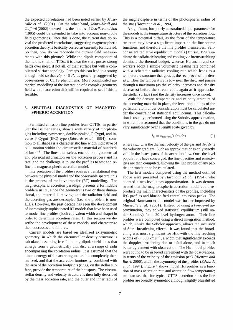
The first models computed using the method outlinedabove were presented byHartmann et al. (1994), whoadopted a two-level atom approximation. It was demon-strated that the magnetospheric accretion model could re-produce the main characteristics of the profiles, includingIPC profiles and blue-shifted central emission peaks. Theoriginal Hartmann et al. model was further improved byMuzerolle et al. (2001). Instead of using a two-level ap-proximation, they solved statistical equilibrium (still un-der Sobolev) for a 20-level hydrogen atom. Their lineprofiles were computed using a direct integration method,which, unlike the Sobolev approach, allows the inclusionof Stark broadening effects. It was found that the broad-ening was most significant for Hα, with the line reachingwidths of∼ 500 km s−1, a width that significantly exceedsthe doppler broadening due to infall alone, and in muchbetter agreement with observation. The Hβ model profileswere found to be in broad agreement with the observations,in terms of the velocity of the emission peak (Alencar andBasri, 2000), and in the asymmetry of the profiles (Edwardset al., 1994). Figure 4 shows model Hα profiles as a func-tion of mass accretion rate and accretion flow temperature;one can see that for typical CTTS accretion rates the lineprofiles are broadly symmetric although slightly blueshifted

7

0

2

4

6

8

6500

K

10-7

0

2

4

6

8

7500

K

0

2

4

6

8

8500

K

-500 0 5000

2

4

6

8

9500

K

0.8

1

1.2

1.4

10-8

0.8

1

1.2

1.4

1

1.5

2

-500 0 500

Velocity (km s-1

)

0

2

4

6

8

0.96

0.98

1

1.02

1.04

10-9

0.6

0.8

1

1.2

0.6

0.8

1

1.2

-500 0 5000.8

1

1.2

1.4

1.6

Fig. 4.— Hα model profiles for a wide range of mass ac-cretion rate and accretion flow maximum temperature (fromKurosawa et al., 2006). The profiles are based on canonicalCTTS parameters (R = 2 R, M = 0.5 M, T = 4000 K)viewed at an inclination of55. The maximum temperatureof the accretion flow is indicated along the left of the figure,while the accretion rate (inM yr−1) is shown along thetop.

– the reduced optical depth for the lower accretion rate mod-els yields the IPC morphology.

Axisymmetric models are obviously incapable of repro-ducing the wide range of variability that is observed in theemission lines of CTTSs (Sect. 4). Although the additionof further free parameters to models naturally renders themmore arbitrary, the observational evidence for introducingsuch parameters is compelling. Perhaps the simplest ex-tension is to break the axisymmetry of the dipole, leavingcurtains of accretion in azimuth – models such as these havebeen proposed by a number of observers attempting to ex-plain variability in CTTSs and are observed in MHD simu-lations (Romanova et al., 2003). Synthetic time-series for aCTTS magnetosphere structured along these lines were pre-sented bySymington et al.(2005a). It was found that somegross characteristics of the observed line profiles were pro-duced using a ‘curtains’ model, although the general levelof variability predicted is larger than that observed, suggest-ing that the magnetosphere may be characterized by a highdegree of axisymmetry, broken by higher-density streamsthat produce the variability.

The emission line profiles of CTTSs often display thesignatures of outflow as well as infall, and recent attemptshave been made to account for this in RT modelling.Alen-car et al. (2005) investigated a dipolar accretion geome-try combined with a disk wind in order to model the lineprofile variability of RW Aur. They discovered that magne-

-500 0 5000

2

4

6

8

I

1

2

3

II

0

5

10

15

20

0

5

10

III

0

5

10

15

-500 0 500B

1

1.5

2

2.5

IV

-500 0 500R

0.8

1

1.2

1.4

1.6

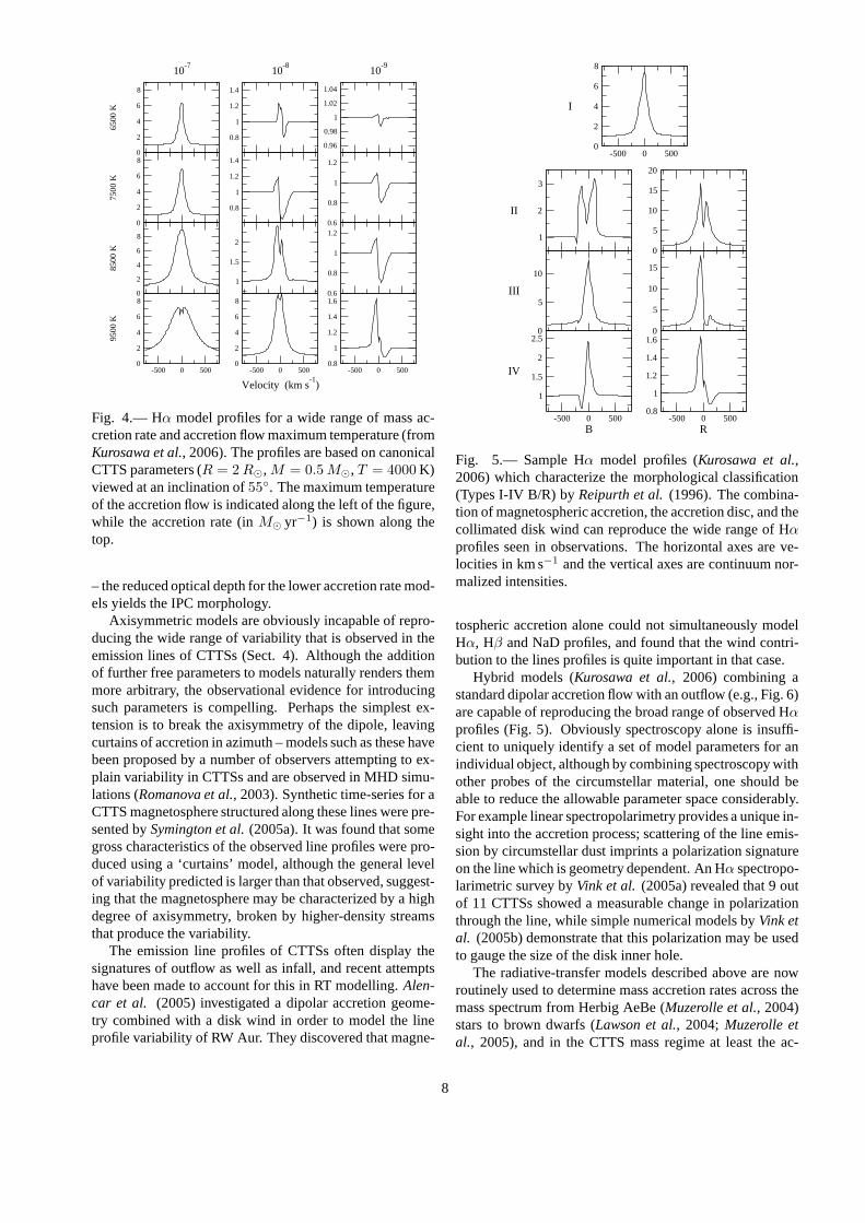
Fig. 5.— Sample Hα model profiles (Kurosawa et al.,2006) which characterize the morphological classification(Types I-IV B/R) byReipurth et al.(1996). The combina-tion of magnetospheric accretion, the accretion disc, and thecollimated disk wind can reproduce the wide range of Hαprofiles seen in observations. The horizontal axes are ve-locities in km s−1 and the vertical axes are continuum nor-malized intensities.

tospheric accretion alone could not simultaneously modelHα, Hβ and NaD profiles, and found that the wind contri-bution to the lines profiles is quite important in that case.

Hybrid models (Kurosawa et al., 2006) combining astandard dipolar accretion flow with an outflow (e.g., Fig. 6)are capable of reproducing the broad range of observed Hαprofiles (Fig. 5). Obviously spectroscopy alone is insuffi-cient to uniquely identify a set of model parameters for anindividual object, although by combining spectroscopy withother probes of the circumstellar material, one should beable to reduce the allowable parameter space considerably.For example linear spectropolarimetry provides a unique in-sight into the accretion process; scattering of the line emis-sion by circumstellar dust imprints a polarization signatureon the line which is geometry dependent. An Hα spectropo-larimetric survey byVink et al. (2005a) revealed that 9 outof 11 CTTSs showed a measurable change in polarizationthrough the line, while simple numerical models byVink etal. (2005b) demonstrate that this polarization may be usedto gauge the size of the disk inner hole.

The radiative-transfer models described above are nowroutinely used to determine mass accretion rates across themass spectrum from Herbig AeBe (Muzerolle et al., 2004)stars to brown dwarfs (Lawson et al., 2004; Muzerolle etal., 2005), and in the CTTS mass regime at least the ac-

8

Fig. 6.— A simulated Hα image of an accreting CTTS withan outflow (log Macc = −8, log Mwind = −9) viewedat an inclination of80. The wind emission is negligiblecompared to the emission from the magnetosphere, and thelower half of the wind is obscured by the circumstellar disk(Kurosawa et al., 2006).

cretion rates derived from RT modelling have been roughlycalibrated against other accretion-rate measures, such astheUV continuum (e.g.,Muzerolle et al., 2001). However, onemust be aware of the simplifying assumptions which un-derlie the models and that must necessarily impact on thevalidity of any quantity derived from them, particularly themass accretion rate. Magnetic field measurements (Sect. 2)and time-series spectroscopy (Sect. 4) clearly show us thatthe geometry of the magnetosphere is far from a pristineaxisymmetric dipole, but instead probably consists of manyazimuthally distributed funnels of accretion, curved by ro-tation and varying in position relative to the stellar surfaceon the timescale of a few stellar rotation periods. Further-more, the temperature of the magnetosphere and the massaccretion rate are degenerate quantities in the models, witha higher temperature magnetosphere producing more lineflux for the same accretion rate. This means that browndwarf models require a much higher accretion stream tem-perature than those of CTTSs in order to produce the ob-served line flux, and although the temperature is grosslyconstrained by the line broadening (which may precludelower temperature streams) the thermal structure of the ac-cretion streams is still a problem. Despite these uncertain-ties, and in defense of the BD models, it should be notedthat the low accretion rates derived are consistent with boththe lack of optical veiling (Muzerolle et al., 2003a) and thestrength of the CaII λ8662 line (Mohanty et al., 2005).

Current models do not match the line core particu-larly well, which is often attributed to a break down ofthe Sobolev approximation; co-moving frame calculations(which are many orders of magnitude more expensive com-putationally) may be required. An additional problem with

current RT modelling is the reliance on fitting a single pro-file – current studies have almost always been limited toHα – one that rarely shows an IPC profile (Edwards et al.,1994;Reipurth et al., 1996), is vulnerable to contaminationby outflows (e.g.,Alencar et al., 2005) and may be signif-icantly spatially extended (Takami et al., 2003). Even inmodelling a single line, it is fair to say that the state-of-the-art is some way short of line profile fitting; the best fits re-ported in the literature may match the observation in termsof peak intensity, equivalent width, or in the line wings,but are rarely convincing reproductions of the observationsin detail. Only by simultaneously fitting several lines mayone have confidence in the models, particularly if thoselines share a common upper/lower level (Hα and Paβ forexample). Although such observations are in the literature(e.g.,Edwards et al., 1994;Folha and Emerson, 2001) theirusefulness is marginalized by the likely presence of signif-icant variability between the epochs of the observations atthe different wavelengths: simultaneous observations of awide range of spectral diagnostics are required. Despitethe caveats described above, line profile modelling remainsa useful (and in the BD case the only) route to the massaccretion rate, and there is real hope that the current fac-tor ∼ 5 uncertainties in mass accretion rates derived fromRT modelling may be significantly reduced in the future.

4. OBSERVATIONAL EVIDENCE FOR MAGNE-TOSPHERIC ACCRETION

Observations seem to globally support the magneto-spheric accretion concept in CTTSs, which includes thepresence of strong stellar magnetic fields, the existence ofan inner magnetospheric cavity of a few stellar radii, mag-netic accretion columns filled with free falling plasma, andaccretion shocks at the surface of the stars. While this sec-tion summarizes the observational signatures of magneto-spheric accretion in T Tauri stars, there is some evidencethat the general picture applies to a much wider range ofmass, from young brown dwarfs (Muzerolle et al., 2005;Mohanty et al., 2005) to Herbig Ae-Be stars (Muzerolle etal., 2004;Calvet et al., 2004;Sorelli et al., 1996).

In recent years, the rapidly growing number of detec-tions of strong stellar magnetic fields at the surface of youngstars seem to put the magnetospheric accretion scenario on arobust ground (see Sect. 2). As expected from the models,given the typical mass accretion rates (10−9 to 10−7 M

yr−1, Gullbring et al., 1998) and magnetic field strengths(2 to 3 kG, Valenti and Johns-Krull, 2004) obtained fromthe observations, circumstellar disk inner holes of about 3-9 R∗ are required to explain the observed line widths ofthe CO fundamental emission, that likely come from gas inKeplerian rotation in the circumstellar disk of CTTSs (Na-jita et al., 2003). There has also been evidence for accre-tion columns through the common occurrence of inverse PCygni profiles with redshifted absorptions reaching several

9

hundred km s−1, which indicates that gas is accreted ontothe star from a distance of a few stellar radii (Edwards etal., 1994).

Accretion shocks are inferred from the rotational mod-ulation of light curves by bright surface spots (Bouvier etal., 1995) and modelling of the light curves suggests hotspots covering about one percent of the stellar surface. Thetheoretical prediction of accretion shocks and its associatedhot excess emission are also supported by accretion shockmodels that successfully reproduce the observed spectralenergy distributions of optical and UV excesses (Calvet andGullbring, 1998;Ardila and Basri, 2000;Gullbring et al.,2000). In these models, the spectral energy distribution ofthe excess emission is explained as a combination of opti-cally thick emission from the heated photosphere below theshock and optically thin emission from the preshock andpostshock regions.Gullbring et al. (2000) also showedthat the high mass accretion rate CTTSs have accretioncolumns with similar values of energy flux as the moder-ate to low mass accretion rate CTTSs, but their accretioncolumns cover a larger fraction of the stellar surface (fillingfactors ranging from less than 1% for low accretors to morethan 10% for the high one). A similar trend was observedby Ardila and Basri(2000) who found, from the study ofthe variability of IUE spectra of BP Tau, that the higher themass accretion rate, the bigger the hot spot size.

Statistical correlations between line fluxes and mass ac-cretion rates predicted by magnetospheric accretion mod-els have also been reported for emission lines in a broadspectral range, from the UV to the near-IR (Johns-Krull etal., 2000;Beristain et al., 2001;Alencar and Basri, 2000;Muzerolle et al., 2001;Folha and Emerson, 2001). How-ever, in recent years, a number of observational results in-dicate that the idealized steady-state axisymmetric dipolarmagnetospheric accretion models cannot account for manyobserved characteristics of CTTSs.

Recent studies showed that accreting systems presentstrikingly large veiling variability in the near-IR (Eiroa etal., 2002;Barsony et al., 2005), pointing to observationalevidence for time variable accretion in the inner disk. More-over, the near-IR veiling measured in CTTSs is often largerthan predicted by standard disk models (Folha and Emer-son, 1999;Johns-Krull and Valenti, 2001). This suggeststhat the inner disk structure is significantly modified by itsinteraction with an inclined stellar magnetosphere and thusdeparts from a flat disk geometry. Alternatively, a “puffed”inner disk rim could result from the irradiation of the in-ner disk by the central star and accretion shock (Natta et al.2001;Muzerolle et al., 2003b). In mildly accreting T Tauristars, the dust sublimation radius computed from irradiationmodels is predicted to lie close to the corotation radius (3-9R∗ ' 0.03-0.08 AU) though direct interferometric measure-ments tend to indicate larger values (0.08-0.2 AU,Akesonet al., 2005).

Observational evidence for an inner disk warp has beenreported byBouvier et al. (1999, 2003) for AA Tau, asexpected from the interaction between the disk and anin-

Fig. 7.— The rotational modulation of the Hα line profileof the CTTS AA Tau (8.2d period). Line profiles are or-dered by increasing rotational phase (top panel number) atdifferent Julian dates (bottom panel number). Note the de-velopment of a high velocity redshifted absorption compo-nent in the profile from phase 0.39 to 0.52, when the funnelflow is seen against the hot accretion shock (fromBouvieret al., in prep.).

clined stellar magnetosphere (see Sect. 5). Inclined mag-netospheres are also necessary to explain the observed pe-riodic variations over a rotational timescale in the emis-sion line and veiling fluxes of a few CTTSs (Johns andBasri, 1995;Petrov et al., 1996; 2001;Bouvier et al., 1999;Batalha et al., 2002). These are expected to arise from thevariations of the projected funnel and shock geometry as thestar rotates. An example can be seen in Fig. 7 that shows theperiodic modulation of the Hα line profile of the CTTS AATau as the system rotates, with the development of a highvelocity redshifted absorption component when the funnelflow is seen against the hot accretion shock. Sometimes,however, multiple periods are observed in the line flux vari-ability and their relationship to stellar rotation is not al-ways clear (e.g.,Alencar and Batalha, 2002;Oliveira et al.,2000). The expected correlation between the line flux fromthe accretion columns, and the continuum excess flux fromthe accretion shock is not always present either (Ardila andBasri, 2000;Batalha et al., 2002), and the correlations pre-dicted by staticdipolar magnetospheric accretion modelsare generally not seen (Johns-Krull and Gafford, 2002).

Winds are generally expected to be seen as forbiddenemission lines or the blueshifted absorption components ofpermitted emission lines. Some permitted emission lineprofiles of high-mass accretion rate CTTSs, however, do notalways look like the ones calculated with magnetosphericaccretion models and this could be in part due to a strongwind contribution to the emission profiles, given the highoptical depth of the wind in these cases (Muzerolle et al.,

10

2001;Alencar et al., 2005). Accretion powered hot windsoriginating at or close to the stellar surface have recentlybeen proposed to exist in CTTSs with high mass accre-tion rates (Edwards et al., 2003). These winds are inferredfrom the observations of P Cygni profiles of the He I line(10780A) that present blueshifted absorptions which ex-tend up to -400 km/s.Matt and Pudritz(2005) have arguedthat such stellar winds can extract a significant amount ofthe star’s angular momentum, thus helping regulate the spinof CTTSs. Turbulence could also be important and help ex-plain the very wide (± 500 km s−1) emission line profilescommonly observed in Balmer and MgII UV lines (Ardilaet al., 2002).

Synoptic studies of different CTTSs highlighted the dy-namical aspect of the accretion/ejection processes, whichonly recently has begun to be studied theoretically by nu-merical simulations (see Sect. 5). The accretion processappears to be time dependent on several timescales, fromhours for non-steady accretion (Gullbring et al., 1996;Alencar and Batalha, 2002;Stempels and Piskunov, 2002;Bouvier et al., 2003) to weeks for rotational modulation(Smith et al., 1999; Johns and Basri, 1995;Petrov et al.,2001), and from months for global instabilities of the mag-netospheric structure (Bouvier et al., 2003) to years forEXor and FUor eruptions (e.g.,Reipurth and Aspin, 2004;Herbig, 1989).

One reason for such a variability could come from theinteraction between the stellar magnetosphere and the inneraccretion disk. In general, magnetospheric accretion mod-els assume that the circumstellar disk is truncated close tothe corotation radius and that field lines threading the diskcorotate with the star. However, many field lines should in-teract with the disk in regions where the star and the diskrotate differentially. Possible evidence has been reportedfor differential rotation between the star and the inner disk(Oliveira et al., 2000) through the presence of an observedtime delay of a few hours between the appearance of highvelocity redshifted absorption components in line profilesformed in different regions of the accretion columns. Thiswas interpreted as resulting from the crossing of an az-imuthally twisted accretion column on the line of sight. An-other possible evidence for twisted magnetic field lines bydifferential rotation leading to reconnection events has beenproposed byMontmerle et al. (2000) for the embeddedprotostellar source YLW 15, based on the observations ofquasi-periodic X-ray flaring. A third possible evidence wasreported byBouvier et al.(2003) for the CTTS AA Tau. Ontimescales of the order of a month, they observed significantvariations in the line and continuum excess flux, indicativeof a smoothly varying mass accretion rate onto the star. Atthe same time, they found a tight correlation between theradial velocity of the blueshifted (outflow) and redshifted(inflow) absorption components in the Hα emission lineprofile. This correlation provides support for a physicalconnection between time dependent inflow and outflow inCTTSs. Bouvier et al. (2003) interpreted the flux and ra-dial velocity variations in the framework of magnetospheric

inflation cycles due to differential rotation between the starand the inner disk, as observed in recent numerical simula-tions (see Sect. 5). The periodicity of such instabilities,aspredicted by numerical models, is yet to be tested observa-tionally and will require monitoring campaigns of chosenCTTSs lasting for several months.

5. NUMERICAL SIMULATIONS OF MAGNETO-SPHERIC ACCRETION

Significant progress has been made in recent years in thenumerical modeling of magnetospheric accretion onto a ro-tating star with a dipolar magnetic field. One of the mainproblems is to find adequate initial conditions which do notdestroy the disk in first few rotations of the star and do notinfluence the simulations thereafter. In particular, one mustdeal with the initial discontinuity of the magnetic field be-tween the disk and the corona, which usually leads to signif-icant magnetic braking of the disk matter and artificially fastaccretion onto the star on a dynamical time-scale. Specificquasi-equilibrium initial conditions were developed, whichhelped to overcome this difficulty (Romanova et al., 2002).In axisymmetric (2D) simulations, the matter of the diskaccretes inward slowly, on a viscous time-scale as expectedin actual stellar disks. The rate of accretion is regulatedby a viscous torque incorporated into the numerical codethrough theα prescription, with typicallyαv = 0.01−0.03.

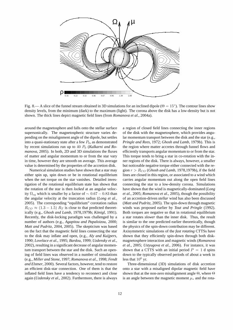
Simulations have shown that the accretion disk is dis-rupted by the stellar magnetosphere at the magnetosphericor truncation radiusRT , where the gas pressure in the diskis comparable to the magnetic pressure,Pram = B2/8π(see Sect. 2). In this region matter is lifted above the diskplane due to the pressure force and falls onto the stellarsurface supersonically along the field lines, forming fun-nel flows (Romanova et al., 2002). The location of the in-ner disk radius oscillates as a result of accumulation andreconnection of the magnetic flux at this boundary, whichblocks or “permits” accretion (see discussion of this issuebelow), thus leading to non-steady accretion through thefunnel flows. Nevertheless, simulations have shown thatthe funnel flow is a quasi-stationary feature during at least50 − 80 rotation periods of the disk at the truncation ra-dius,P0, and recent simulations with improved numericalschemes indicate that this structure survives for more than1, 000 P0 (Long et al., 2005). Axisymmetric simulationsthus confirmed the theoretical ideas regarding the structureof the accretion flow around magnetized CTTSs. As a nextstep, similar initial conditions were applied to full 3D simu-lations of disk accretion onto a star with aninclineddipole,a challenging problem which required the development ofnew numerical methods (e.g., the “inflated cube” grid, cf.Koldoba et al., 2002;Romanova et al., 2003, 2004a). Sim-ulations have shown that the disk is disrupted at the trunca-tion radiusRT , as in the axisymmetric case, but the mag-netospheric flow to the star is more complex. Matter flows

11

0.16 0.22 0.32 0.46 0.67 0.96 1.39 2.00

µ

ρ

Ω

Fig. 8.— A slice of the funnel stream obtained in 3D simulations for an inclined dipole (Θ = 15). The contour lines showdensity levels, from the minimum (dark) to the maximum (light). The corona above the disk has a low-density but is notshown. The thick lines depict magnetic field lines (fromRomanova et al., 2004a).

around the magnetosphere and falls onto the stellar surfacesupersonically. The magnetospheric structure varies de-pending on the misalignment angle of the dipole, but settlesinto a quasi-stationary state after a fewP0, as demonstratedby recent simulations run up to40 P0 (Kulkarni and Ro-manova, 2005). In both, 2D and 3D simulations the fluxesof matter and angular momentum to or from the star varyin time, however they are smooth on average. This averagevalue is determined by the properties of the accretion disk.

Numerical simulation studies have shown that a star mayeither spin up, spin down or be in rotational equilibriumwhen the net torque on the star vanishes. Detailed inves-tigation of the rotational equilibrium state has shown thatthe rotation of the star is thenlockedat an angular veloc-ity Ωeq which is smaller by a factor of∼ 0.67 − 0.83 thanthe angular velocity at the truncation radius (Long et al.,2005). The corresponding “equilibrium” corotation radiusRCO ≈ (1.3 − 1.5) RT is close to that predicted theoret-ically (e.g.,Ghosh and Lamb, 1978,1979b;Konigl, 1991).Recently, the disk-locking paradigm was challenged by anumber of authors (e.g.,Agapitou and Papaloizou, 2000;Matt and Pudritz, 2004, 2005). The skepticism was basedon the fact that the magnetic field lines connecting the starto the disk may inflate and open, (e.g.,Aly and Kuijpers,1990;Lovelace et al., 1995;Bardou, 1999;Uzdensky et al.,2002), resulting in a significant decrease of angular momen-tum transport between the star and the disk. Such an open-ing of field lines was observed in a number of simulations(e.g.,Miller and Stone, 1997;Romanova et al., 1998;Fendtand Elstner, 2000). Several factors, however, tend to restorean efficient disk-star connection. One of them is that theinflated field lines have a tendency to reconnect and closeagain (Uzdensky et al., 2002). Furthermore, there is always

a region of closed field lines connecting the inner regionsof the disk with the magnetosphere, which provides angu-lar momentum transport between the disk and the star (e.g.,Pringle and Rees, 1972;Ghosh and Lamb, 1979b). This isthe region where matter accretes through funnel flows andefficiently transports angular momentum to or from the star.This torque tends to bring a star in co-rotation with the in-ner regions of the disk. There is always, however, a smallerbut noticeable negative torque either connected with the re-gionr > RCO (Ghosh and Lamb, 1978,1979b), if the fieldlines are closed in this region, or associated to a wind whichcarries angular momentum out along the open field linesconnecting the star to a low-density corona. Simulationshave shown that the wind is magnetically-dominated (Longet al., 2005;Romanova et al., 2005), though the possibilityof an accretion-drivenstellar wind has also been discussed(Matt and Pudritz, 2005). The spin-down through magneticwinds was proposed earlier byTout and Pringle(1992).Both torques are negative so that in rotational equilibriuma star rotatesslower than the inner disk. Thus, the resultis similar to the one predicted earlier theoretically, thoughthe physics of the spin-down contribution may be different.Axisymmetric simulations of thefast rotatingCTTSs haveshown that they efficiently spin-down through both disk-magnetosphere interaction and magnetic winds (Romanovaet al., 2005;Ustyugova et al., 2006). For instance, it wasshown that a CTTS with an initial periodP = 1 d spinsdown to the typically observed periods of about a week inless that106 yr.

Three-dimensional (3D) simulations of disk accretiononto a star with a misaligned dipolar magnetic field haveshown that at the non-zero misalignment angleΘ, whereΘis an angle between the magnetic momentµ∗ and the rota-

12

X

Y

Z

µX

Y

Z

µ

Fig. 9.— 3D simulations show that matter accretes onto thestar through narrow, high density streams (right panel) sur-rounded by lower density funnel flows that blanket nearlythe whole magnetosphere (left panel).

Θ=30ο Θ=60ο Θ=90ο

+

Ωµ

Θ=90ο

+

Ωµ

Θ=30ο

+

Ωµ

Θ=60ο

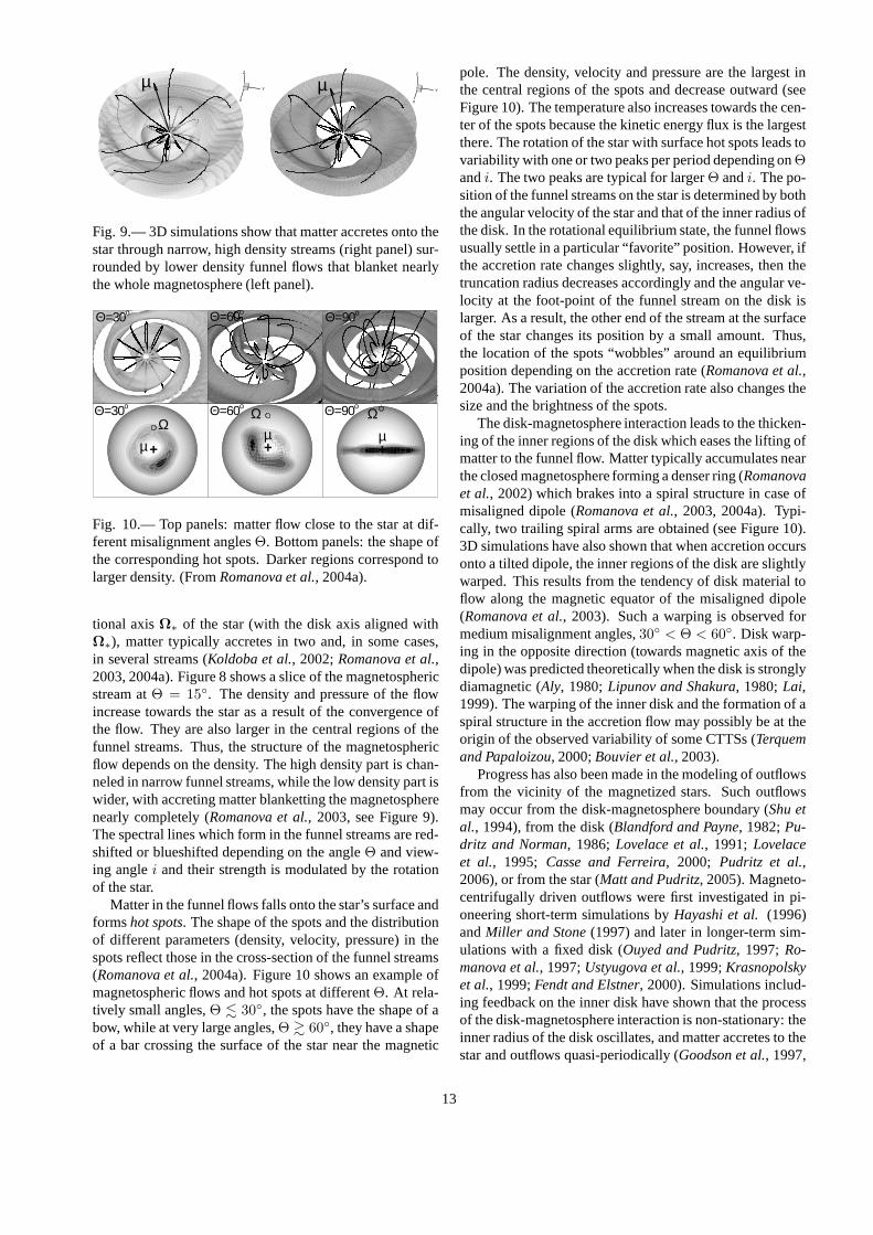
Fig. 10.— Top panels: matter flow close to the star at dif-ferent misalignment anglesΘ. Bottom panels: the shape ofthe corresponding hot spots. Darker regions correspond tolarger density. (FromRomanova et al., 2004a).

tional axisΩ∗ of the star (with the disk axis aligned withΩ∗), matter typically accretes in two and, in some cases,in several streams (Koldoba et al., 2002;Romanova et al.,2003, 2004a). Figure 8 shows a slice of the magnetosphericstream atΘ = 15. The density and pressure of the flowincrease towards the star as a result of the convergence ofthe flow. They are also larger in the central regions of thefunnel streams. Thus, the structure of the magnetosphericflow depends on the density. The high density part is chan-neled in narrow funnel streams, while the low density part iswider, with accreting matter blanketting the magnetospherenearly completely (Romanova et al., 2003, see Figure 9).The spectral lines which form in the funnel streams are red-shifted or blueshifted depending on the angleΘ and view-ing anglei and their strength is modulated by the rotationof the star.

Matter in the funnel flows falls onto the star’s surface andformshot spots. The shape of the spots and the distributionof different parameters (density, velocity, pressure) in thespots reflect those in the cross-section of the funnel streams(Romanova et al., 2004a). Figure 10 shows an example ofmagnetospheric flows and hot spots at differentΘ. At rela-tively small angles,Θ . 30, the spots have the shape of abow, while at very large angles,Θ & 60, they have a shapeof a bar crossing the surface of the star near the magnetic

pole. The density, velocity and pressure are the largest inthe central regions of the spots and decrease outward (seeFigure 10). The temperature also increases towards the cen-ter of the spots because the kinetic energy flux is the largestthere. The rotation of the star with surface hot spots leads tovariability with one or two peaks per period depending onΘandi. The two peaks are typical for largerΘ andi. The po-sition of the funnel streams on the star is determined by boththe angular velocity of the star and that of the inner radius ofthe disk. In the rotational equilibrium state, the funnel flowsusually settle in a particular “favorite” position. However, ifthe accretion rate changes slightly, say, increases, then thetruncation radius decreases accordingly and the angular ve-locity at the foot-point of the funnel stream on the disk islarger. As a result, the other end of the stream at the surfaceof the star changes its position by a small amount. Thus,the location of the spots “wobbles” around an equilibriumposition depending on the accretion rate (Romanova et al.,2004a). The variation of the accretion rate also changes thesize and the brightness of the spots.

The disk-magnetosphere interaction leads to the thicken-ing of the inner regions of the disk which eases the lifting ofmatter to the funnel flow. Matter typically accumulates nearthe closed magnetosphere forming a denser ring (Romanovaet al., 2002) which brakes into a spiral structure in case ofmisaligned dipole (Romanova et al., 2003, 2004a). Typi-cally, two trailing spiral arms are obtained (see Figure 10).3D simulations have also shown that when accretion occursonto a tilted dipole, the inner regions of the disk are slightlywarped. This results from the tendency of disk material toflow along the magnetic equator of the misaligned dipole(Romanova et al., 2003). Such a warping is observed formedium misalignment angles,30 < Θ < 60. Disk warp-ing in the opposite direction (towards magnetic axis of thedipole) was predicted theoretically when the disk is stronglydiamagnetic (Aly, 1980;Lipunov and Shakura, 1980;Lai,1999). The warping of the inner disk and the formation of aspiral structure in the accretion flow may possibly be at theorigin of the observed variability of some CTTSs (Terquemand Papaloizou, 2000;Bouvier et al., 2003).

Progress has also been made in the modeling of outflowsfrom the vicinity of the magnetized stars. Such outflowsmay occur from the disk-magnetosphere boundary (Shu etal., 1994), from the disk (Blandford and Payne, 1982;Pu-dritz and Norman, 1986;Lovelace et al., 1991; Lovelaceet al., 1995; Casse and Ferreira, 2000; Pudritz et al.,2006), or from the star (Matt and Pudritz, 2005). Magneto-centrifugally driven outflows were first investigated in pi-oneering short-term simulations byHayashi et al. (1996)andMiller and Stone(1997) and later in longer-term sim-ulations with a fixed disk (Ouyed and Pudritz, 1997;Ro-manova et al., 1997;Ustyugova et al., 1999;Krasnopolskyet al., 1999;Fendt and Elstner, 2000). Simulations includ-ing feedback on the inner disk have shown that the processof the disk-magnetosphere interaction is non-stationary:theinner radius of the disk oscillates, and matter accretes to thestar and outflows quasi-periodically (Goodson et al., 1997,

13

1999; Hirose et al., 1997; Matt et al., 2002; Kato et al.,2004;Romanova et al., 2004b;Von Rekowski and Branden-burg, 2004; Romanova et al., 2005), as predicted byAlyand Kuijpers(1990). The characteristic timescale of vari-ability is determined by a number of factors, including thetime-scale of diffusive penetration of the inner disk matterthrough the external regions of the magnetosphere (Good-son and Winglee, 1999). It was earlier suggested that re-connection of the magnetic flux at the disk-magnetosphereboundary may lead to X-ray flares in CTTSs (Hayashi etal., 1996; Feigelson and Montmerle, 1999) and evidencefor very large flaring structures has been recently reportedby Favata et al.(2005).

So far simulations were done for a dipolar magneticfield. Observations suggest a non-dipolar magnetic fieldnear the stellar surface (see Sect. 2, and also, e.g.,Safier,1998;Kravtsova and Lamzin, 2003;Lamzin, 2003;Smirnovet al., 2005). If the dipole component dominates on thelarge scale, many properties of magnetospheric accretionwill be similar to those described above, including the struc-ture of the funnel streams and their physical properties.However, the multipolar component will probably controlthe flow near the stellar surface, possibly affecting the shapeand the number of hot spots. Simulations of accretion to astar with a multipolar magnetic field are more complicated,and should be done in the future.

6. CONCLUSIONS

Recent magnetic field measurements in T Tauri starssupport the view that the accretion flow from the inner diskonto the star is magnetically controlled. While typical val-ues of 2.5 kG are obtained for photospheric fields, it alsoappears that the field topology is likely complex on thesmall-scales (R≤R?), while on the larger scale (R>>R?)a globally more organized but weaker (∼0.1 kG) magneticcomponent dominates. This structure is thought to inter-act with the inner disk to yield magnetically-channeled ac-cretion onto the star. Observational evidence for magneto-spheric accretion in classical T Tauri star is robust (innerdisk truncation, hot spots, line profiles) and the rotationalmodulation of accretion/ejection diagnostics observed insome systems suggests that the stellar magnetosphere ismoderately inclined relative to the star’s rotational axis. Re-alistic 3D numerical models have capitalized on the obser-vational evidence to demonstrate that many properties ofaccreting T Tauri stars could be interpreted in the frame-work of magnetically-controlled accretion. One of the mostconspicuous properties of young stars is their extreme vari-ability on timescales ranging from hours to months, whichcan sometimes be traced to instabilities or quasi-periodicphenomena associated to the magnetic star-disk interaction.

Much work remains to be done, however, before reach-ing a complete understanding of this highly dynamical andtime variable process. Numerical simulations still have to

incorporate field geometries more complex than a tilteddipole, e.g., the superposition of a large-scale dipolar orquadrupolar field with multipolar fields at smaller scales.The modeling of emission line profiles now starts to com-bine radiative transfer computations in both accretion fun-nel flows and associated mass loss flows (disk winds, stellarwinds), which indeed appears necessary to account for thelarge variety of line profiles exhibited by CTTSs. Thesemodels also have to address the strong line profile vari-ability which occurs on a timescale ranging from hours toweeks in accreting T Tauri stars. These foreseen devel-opments must be driven by intense monitoring of typicalCTTSs on all timescales from hours to years, which com-bines photometry, spectroscopy and polarimetry in variouswavelength domains. This will provide strong constraintson the origin of the variability of the various components ofthe star-disk interaction process (e.g., inner disk in the near-IR, funnel flows in emission lines, hot spots in the opticalor UV, magnetic reconnections in X-rays, etc.).

The implications of the dynamical nature of magneto-spheric accretion in CTTSs are plentiful and remain to befully explored. They range from the evolution of stellarangular momentum during the pre-main sequence phase(e.g., Agapitou and Papaloizou, 2000), the origin of in-flow/ouflow short term variability (e.g.,Woitas et al., 2002;Lopez-Martin et al., 2003), the modeling of the near in-frared veiling of CTTSs and of its variations, both of whichwill be affected by a non planar and time variable inner diskstructure (e.g.,Carpenter et al., 2001;Eiroa et al., 2002),and possibly the halting of planet migration close to the star(Lin et al., 1996).

Acknowledgments. SA acknowledges financial sup-port from CNPq through grant 201228/2004-1. Work ofMMR was supported by the NASA grants NAG5-13060,NAG5-13220, and by the NSF grants AST-0307817 andAST-0507760.

REFERENCES

Agapitou V. and Papaloizou J. C. B. (2000)Mon. Not. R. Astron.Soc., 317, 273-288.

Akeson R. L., Boden A. F., Monnier J. D., Millan-Gabet R., Be-ichman C., et al. (2005)Astrophys. J., 635, 1173-1181.

Alencar S. H. P. and Basri G. (2000)Astron. J., 119, 1881-1900.Alencar S. H. P. and Batalha C. (2002)Astrophys. J., 571, 378-

393.Alencar S. H. P., Basri G., Hartmann L., and Calvet N. (2005)

Astron. Astrophys., 440, 595-608.Aly J. J. (1980)Astron. Astrophys., 86, 192-197.Aly J. J. and Kuijpers J. (1990)Astron. Astrophys., 227, 473-482.Andre P. (1987) InProtostars and Molecular Clouds(T. Mont-

merle and C. Bertout, eds.), pp.143-187. CEA, Saclay.Ardila D. R. and Basri G. (2000)Astrophys. J., 539, 834-846.Ardila D. R., Basri G., Walter F. M., Valenti J. A., and Johns-Krull

C. M. (2002)Astrophys. J., 567, 1013-1027.Bardou A. (1999)Mon. Not. R. Astron. Soc., 306, 669-674.Barsony M., Ressler M. E., and Marsh K. A. (2005)Astrophys. J.,

630, 381-399.

14

Basri G. and Bertout C. (1989)Astrophys. J., 341, 340-358.Basri G., Marcy G. W., and Valenti J. A. (1992)Astrophys. J., 390,

622-633.Batalha C., Batalha N. M., Alencar S. H. P., Lopes D. F., and

Duarte E. S. (2002)Astrophys. J., 580, 343-357.Beristain G., Edwards S., and Kwan J. (2001)Astrophys. J., 551,

1037-1064.Blandford R. D. and Payne D. G. (1982)Mon. Not. R. Astron.

Soc., 199, 883-903.Borra E. F., Edwards G., and Mayor M. (1984)Astrophys. J., 284,

211-222.Bouvier J., Chelli A., Allain S., Carrasco L., Costero R., etal.

(1999)Astron. Astrophys., 349, 619-635.Bouvier J., Grankin K. N., Alencar S. H. P., Dougados C.,

Fernandez M., et al. (2003)Astron. Astrophys., 409, 169-192.Bouvier J., Cabrit S., Fenandez M., Martin E. L., and Matthews

J. M. (1993)Astron. Astrophys., 272, 176-206.Bouvier J., Covino E., Kovo O., Martın E. L., Matthews J. M.,et

al. (1995)Astron. Astrophys., 299, 89-107.Brown D. N. and Landstreet J. D. (1981)Astrophys. J., 246, 899-

904.Calvet N. and Gullbring E. (1998)Astrophys. J., 509, 802-818.Calvet N., Muzerolle J., Briceno C., Fernandez J., Hartmann L., et

al. (2004)Astron. J., 128, 1294-1318.Camenzind M. (1990)Rev. Mex. Astron. Astrofis., 3, 234-265.Carpenter J. M., Hillenbrand L. A., and Skrutskie M. F. (2001)

Astron. J., 121, 3160-3190.Casse F. and Ferreira J. (2000)Astron. Astrophys. 361, 1178-1190Collier Cameron A. C. and Campbell C. G. (1993)Astron. Astro-

phys., 274, 309-318.Daou A. G., Johns–Krull C. M., and Valenti J. A. (2006)Astron.

J., 131, 520-526.Donati J.-F., Semel M., Carter B. D., Rees D. E., and Collier

Cameron A. (1997)Mon. Not. R. Astron. Soc., 291, 658-682.Edwards S., Hartigan P., Ghandour L., and Andrulis C. (1994)

Astron. J., 108, 1056-1070.Edwards S., Fischer W., Kwan J., Hillenbrand L., and Dupree

A. K. (2003)Astrophys. J., 599, L41-L44.Eiroa, C., Oudmaijer R. D., Davies J. K., de Winter D., Garzn F.,

et al. (2002)Astron. Astrophys., 384, 1038-1049.Favata F., Flaccomio E., Reale F., Micela G., Sciortino S., et al.

(2005)Astrophys. J. Suppl., 160, 469-502.Feigelson E. D. and Montmerle T. (1999)Ann. Rev. Astron. As-

trophys., 37, 363-408.Fendt C. and Elstner D. (2000)Astron. Astrophys., 363, 208-222.Folha D. F. M. and Emerson J. P. (1999)Astron. Astrophys., 352,

517-531.Folha D. F. M. and Emerson J. P. (2001)Astron. Astrophys., 365,

90-109.Ghosh P. and Lamb F. K. (1978)Astrophys. J., 223, L83-L87.Ghosh P. and Lamb F. K. (1979a)Astrophys. J., 232, 259-276.Ghosh P. and Lamb F. K. (1979b)Astrophys. J., 234, 296-316.Goodson A. P. and Winglee R. M. (1999)Astrophys. J., 524, 159-

168.Goodson A. P., Winglee R. M., and Bohm K.-H. (1997)Astro-

phys. J., 489, 199-209.Goodson A. P., Bohm K.-H. and Winglee R. M. (1999)Astrophys.

J., 524, 142-158.Guenther E. W., Lehmann H., Emerson J. P., and Staude J. (1999)

Astron. Astrophys., 341, 768-783.Gullbring E., Barwig H., Chen P. S., Gahm G. F., and Bao M. X.

(1996)Astron. Astrophys., 307, 791-802.

Gullbring E., Hartmann L., Briceno C., and Calvet N. (1998)As-trophys. J., 492, 323-341.

Gullbring E., Calvet N., Muzerolle J., and Hartmann L. (2000)Astrophys. J., 544, 927-932.

Hartigan P., Edwards S., and Ghandour L. (1995)Astrophys. J.,452, 736-768.

Hartmann L., Hewett R., and Calvet N. (1994)Astrophys. J., 426,669-687.

Hayashi M. R., Shibata K., and Matsumoto R. (1996)Astrophys.J., 468, L37-L40.

Herbig G. H. (1989) InLow Mass Star Formation and Pre-mainSequence Objects(B. Reipurth, ed.), pp.233-246. ESO, Garch-ing.

Herbst W., Bailer-Jones C. A. L., Mundt R., Meisenheimer K.,andWackermann R. (2002)Astron. Astrophys., 396, 513-532.

Hirose S., Uchida Y., Shibata K., and Matsumoto R. (1997)Pub.Astron. Soc. Jap., 49, 193-205.

Jardine M., Collier Cameron A., and Donati J.-F. (2002)Mon. Not.R. Astron. Soc., 333, 339-346.

Johns C. M. and Basri G. (1995)Astrophys. J., 449, 341-364.Johns–Krull C. M. and Gafford A. D. (2002)Astrophys. J., 573,

685-698.Johns–Krull C. M. and Valenti J. A. (2001)Astrophys. J., 561,

1060-1073.Johns–Krull C. M., Valenti J. A., Hatzes A. P., and Kanaan A.

(1999a)Astrophys. J., 510, L41-L44.Johns–Krull C. M., Valenti J. A., and Koresko C. (1999b)Astro-

phys. J., 516, 900-915.Johns-Krull C. M., Valenti J. A., and Linsky J. L. (2000)Astro-

phys. J., 539, 815-833.Johns–Krull C. M., Valenti J. A., Saar S. H., and Hatzes A. P.

(2001) InMagnetic Fields Across the Hertzsprung-Russell Di-agram(G. Mathys et al., eds.), pp. 527-532. ASP Conf. Series,San Francisco.

Johns–Krull C. M., Valenti J. A., and Saar S. H. (2004)Astrophys.J., 617, 1204-1215.

Johnstone R. M. and Penston M. V. (1986)Mon. Not. R. Astron.Soc., 219, 927-941.

Johnstone R. M. and Penston M. V. (1987)Mon. Not. R. Astron.Soc., 227, 797-800.

Kato Y., Hayashi M. R. and Matsumoto R. (2004)Astrophys. J.,600, 338-342.

Koide S., Shibata K., and Kudoh T. (1999)Astrophys. J., 522,727-752.

Koldoba A. V., Romanova M. M., Ustyugova G. V., and LovelaceR. V. E. (2002)Astrophys. J., 576, L53 -L56.

Konigl. A. (1991)Astrophys. J., 370, L39-L43.Krasnopolsky R., Li Z.-Y., and Blandford R. (1999)Astrophys. J.,

526, 631-642.Kravtsova A. S. and Lamzin S. A. (2003)Astron. Lett., 29, 612-

620.Kulkarni A. K. and Romanova M. M. (2005)Astrophys. J., 633,

349-357.Kurosawa R., Harries T. J., and Symington N. H. (2006)Mon. Not.

R. Astron. Soc., submittedLai D. (1999)Astrophys. J., 524, 1030-1047.Lamzin S. A. (2003)Astron. Reports, 47, 498-510.Lawson W. A., Lyo A.-R., and Muzerolle J. (2004)Mon. Not. R.

Astron. Soc., 351, L39-L43.Lin D. N. C., Bodenheimer P., and Richardson D. C. (1996)Na-

ture, 380, 606-607.Lipunov V. M. and Shakura N. I. (1980)Soviet Astronomy Letters,

15

6, 14-17.Long M., Romanova M. M., and Lovelace R. V. E. (2005)Astro-

phys. J., 634, 1214-1222.Lopez-Martın L., Cabrit S., and Dougados C. (2003)Astron. As-

trophys., 405, L1-L4.Lovelace R. V. E., Berk H. L., and Contopoulos J. (1991)Astro-

phys. J., 379, 696-705.Lovelace R. V. E., Romanova M. M., and Bisnovatyi-Kogan G. S.

(1995)Mon. Not. R. Astron. Soc., 275, 244-254.Martin S. C., (1996)Astrophys. J., 470, 537-550.Matt S. and Pudritz R. E. (2004)Astrophys. J., 607, L43-L46.Matt S. and Pudritz R. E. (2005)Astrophys. J., 632, L135-L138.Matt S., Goodson A. P., Winglee R. M., and Bohm K.-H. (2002)

Astrophys. J., 574, 232-245.Menard F. and Bertout C. (1999) InThe Origin of Stars and Plan-

etary Systems(C. J. Lada and N. D. Kylafis, eds), pp.341.Kluwer Academic Publishers.

Miller K. A. and Stone J. M. (1997)Astrophys. J., 489, 890-902.Mohanty S. M., Jayawardhana R., and Basri G. (2005)Astrophys.

J., 626, 498-522.Montmerle T., Koch-Miramond L., Falgarone E., and Grindlay

J. E. (1983)Astrophys. J., 269, 182-201.Montmerle T., Grosso N., Tsuboi Y., and Koyama K. (2000)As-

trophys. J., 532, 1097-1110.Muzerolle J., Calvet N., and Hartmann L. (2001)Astrophys. J.,

550, 944-61.Muzerolle J., Hillenbrand L., Calvet N., Briceno C., and Hartmann

L. (2003a)Astrophys. J., 592, 266-281.Muzerolle J., Calvet N., Hartmann L., and D’Alessio P. (2003b)

Astrophys. J., 597, L149-L152.Muzerolle J., D’Alessio P., Calvet N., and Hartmann L. (2004)

Astrophys. J., 617, 406-417.Muzerolle J., Luhman K. L., Briceno C., Hartmann L., and Calvet

N. (2005)Astrophys. J., 625, 906-912.Najita J., Carr J. S. and Mathieu R. D. (2003)Astrophys. J., 589,

931-952.Natta A., Prusti T., Neri R., Wooden D., Grinin V. P., and Man-

nings V. (2001)Astron. Astrophys., 371, 186-197Oliveira J. M. Foing, B. H., van Loon J. T., and Unruh Y. C. (2000)

Astron. Astrophys., 362, 615-627.Ostriker E. C. and Shu F. H. (1995)Astrophys. J., 447, 813-828.Ouyed R. and Pudritz R. E. (1997)Astrophys. J., 482, 712-732.ud Petit P., Donati J.-F., Wade G. A., Landstreet J. D., BagnuloS.,

et al. (2004)Mon. Not. R. Astron. Soc., 348, 1175-1190.Petrov P. P., Gullbring E., Ilyin I., Gahm G. F., Tuominen I.,et al.

(1996)Astron. Astrophys., 314, 821-834.Petrov P. P., Gahm G. F., Gameiro J. F., Duemmler R., Ilyin I. V.,

et al. (2001)Astron. Astrophys., 369, 993-1008.Pringle J. E. and Rees M. J. (1972)Astron. Astrophys., 21, 1P-9P.Pudritz R. E. and Norman C. A. (1986)Astrophys. J., 301, 571-

586.Pudritz R. E., Rogers C. S., and Ouyed R. (2006)Mon. Not. R.

Astron. Soc., 365, 1131-1148.Reipurth B. and Aspin C. (2004)Astrophys. J., 608, L65-L68.Reipurth B., Pedrosa A., and Lago M. T. V. T. (1996)Astron. As-

trophys. Suppl., 120, 229-256.Romanova M. M., Ustyugova G. V., Koldoba A. V., Chechetkin

V. M., and Lovelace R. V. E. (1997)Astrophys. J., 482, 708-711.

Romanova M. M., Ustyugova G. V., Koldoba A. V., ChechetkinV. M., and Lovelace R. V. E. (1998)Astrophys. J., 500, 703-713.

Romanova M. M., Ustyugova G. V., Koldoba A. V., and LovelaceR. V. E. (2002)Astrophys. J., 578, 420-438.

Romanova M. M., Ustyugova G. V., Koldoba A. V., Wick J. V.,and Lovelace R. V. E. (2003)Astrophys. J., 595, 1009-1031.

Romanova M. M., Ustyugova G. V., Koldoba A. V., and LovelaceR. V. E. (2004a)Astrophys. J., 610, 920-932.

Romanova M. M., Ustyugova G. V., Koldoba A. V., and LovelaceR. V. E. (2004b)Astrophys. J., 616, L151 -L154.

Romanova M. M., Ustyugova G. V., Koldoba A. V., and LovelaceR. V. E. (2005)Astrophys. J., 635, L165-L168.

Safier P. N. (1998)Astrophys. J., 494, 336-341.Shu F., Najita J., Ostriker E., Wilkin F., Ruden S., and Lizano S.

(1994)Astrophys. J., 429, 781-796.Smirnov D. A., Lamzin S. A., Fabrika S. N., and Valyavin G. G.

(2003)Astron. Astrophys., 401, 1057-1061.Smirnov D. A., Lamzin S. A., Fabrika S. N., and Chuntonov G. A.

(2004)Astron. Lett., 30, 456-460.Smirnov D. A., Romanova M. M., and Lamzin S. A. (2005)As-

tron. Lett., 31, 335-339.Smith K. W., Lewis G. F., Bonnell I. A., Bunclark P. S., and Emer-

son J. P. (1999)Mon. Not. R. Astron. Soc., 304, 367-388.Smith K., Pestalozzi M., Gudel M., Conway J., and Benz A. O.

(2003)Astron. Astrophys., 406, 957-967.Sorelli C., Grinin V. P., and Natta A. (1996)Astron. Astrophys.,

309, 155-162.Stempels H. C. and Piskunov N. (2002)Astron. Astrophys., 391,

595-608.Symington N. H., Harries T. J., and Kurosawa R. (2005a)Mon.

Not. R. Astron. Soc., 356, 1489-1500.Symington N. H., Harries T. J., Kurosawa R., and Naylor T.

(2005b)Mon. Not. R. Astron. Soc., 358, 977-984.Takami M., Bailey J., and Chrysostomou A. (2003)Astron. Astro-

phys., 397, 675-984.Terquem C. and Papaloizou J. C. B. (2000)Astron. Astrophys.,

360, 1031-1042.Tout C. A. and Pringle J. E. (1992)Mon. Not. R. Astron. Soc.,

256, 269-276.Ustyugova G. V., Koldoba A. V., Romanova M. M., and Lovelace

R. V. E. (1999)Astrophys. J., 516, 221-235.Ustyugova, G.V., Koldoba, A.V., Romanova, M.M., and Lovelace,

R.V.E. (2006).Astrophys. J., in pressUzdensky D. A., Konigl A., and Litwin C. (2002)Astrophys. J.,

565, 1191-1204.Valenti J. A. and Johns-Krull C. M. (2004)Astrophys. Sp. Sci.

Ser., 292, 619-629.Valenti J. A., Basri G., and Johns C. M. (1993)Astron. J., 106,

2024-2050.Vink J. S., Drew J. E., Harries T. J., Oudmaijer R. D., and Unruh

Y. (2005a)Mon. Not. R. Astron. Soc., 359, 1049-1064.Vink J. S., Harries T. J., and Drew J. E. (2005b)Astron. Astrophys.,

430, 213-222.Vogt S. S. (1980)Astrophys. J., 240, 567-584.von Rekowski B. and Brandenburg A. (2004)Astron. Astrophys.,

420, 17-32.Warner B. (2004)Publ. Astron. Soc. Pac., 116, 115-132Woitas J., Ray T. P., Bacciotti F., Davis C. J., and Eisloffel J.

(2002)Astrophys. J., 580, 336-342.Yang H., Johns–Krull C. M., and Valenti J. A. (2005)Astrophys.

J., 635, 466-475.

16