Magneto-quantum-nanomechanics: ultra-high Q

levitated mechanical oscillators

M. Cirio1,†, J. Twamley1, G.K. Brennen1.1Centre for Engineered Quantum Systems, Department of Physics and Astronomy,

Macquarie University, North Ryde, NSW 2109, Australia

E-mail: mauro.cirio@students.mq.edu.au

Abstract. Engineering nano-mechanical quantum systems possessing

ultra-long motional coherence times allow for applications in ultra-sensitive

quantum sensing, motional quantum memories and motional interfaces

between other carriers of quantum information such as photons, quantum

dots and superconducting systems. To achieve ultra-high motional Q one

must work hard to remove all forms of motional noise and heating. We

examine a magneto-nanomechanical quantum system that consists of a 3D

arrangement of miniature superconducting loops which is stably levitated in

a static inhomogenous magnetic field. The resulting motional Q is limited

by the tiny decay of the supercurrent in the loops and may reach up to

Q ∼ 1010. We examine the classical and quantum dynamics of the levitating

superconducting system and prove that it is stably trapped and can achieve

motional oscillation frequencies of several tens of MHz. By inductively

coupling this levitating object to a nearby flux qubit we further show that

by driving the qubit one can cool the motion of the levitated object and in

the case of resonance, this can cool the vertical motion of the object close

to its ground state.

† Author to whom any correspondence should be addressed.

arX

iv:1

112.

5208

v1 [

quan

t-ph

] 2

2 D

ec 2

011

2

Contents

1 Introduction 2

2 Toy Model 3

3 Model 4

3.1 Resonator . . . . . . . . . . . . . . . . . . . . . . . . . . . . . . . . . . . 5

3.2 Qubit . . . . . . . . . . . . . . . . . . . . . . . . . . . . . . . . . . . . . 8

3.3 Interaction . . . . . . . . . . . . . . . . . . . . . . . . . . . . . . . . . . . 8

4 Cooling 9

4.1 Cooling scheme A: Introduction . . . . . . . . . . . . . . . . . . . . . . . 9

4.1.1 Low Temperature Regime . . . . . . . . . . . . . . . . . . . . . . 10

4.1.2 High Temperature Regime . . . . . . . . . . . . . . . . . . . . . . 11

4.2 Cooling scheme B . . . . . . . . . . . . . . . . . . . . . . . . . . . . . . . 11

5 Results 12

5.1 Classical Motion . . . . . . . . . . . . . . . . . . . . . . . . . . . . . . . 12

5.2 Superconductivity and Dissipation . . . . . . . . . . . . . . . . . . . . . . 14

5.3 Coupling between the resonator and the flux qubit. . . . . . . . . . . . . 15

5.4 Cooling of the motional resonator. . . . . . . . . . . . . . . . . . . . . . . 15

5.4.1 Cooling scheme A. . . . . . . . . . . . . . . . . . . . . . . . . . . 15

5.4.2 Cooling scheme B. . . . . . . . . . . . . . . . . . . . . . . . . . . 18

6 Conclusions 19

7 Acknowledgements 20

8 Parameter Table 21

Appendix AHigh temperature regime final occupation number 21

References 24

1. Introduction

Recently there has been considerable effort towards mapping the boundary between the

classical and the quantum world by exploring the physics of mesoscopic and macroscopic

mechanical systems. From an applications point of view, as precision measurement

of position and acceleration generally involve some kind of motion, the necessity of

building smaller and more sensitive devices has required a more careful exploration of

the classical-quantum limit.

The possibility to couple, control and measure micro-mechanical motion in a wide

range of different physical systems leads to new experimental applications in different

3

fields such as measuring forces between individual biomolecules [1, 2, 3], magnetic

forces from single spins [4], perturbations due to the mass fluctuations involving single

atoms and molecules [5], pressure [6] and acceleration [6], fundamental constants

[7], small changes in electrical charge [8], gravitational wave detection [9], as well as

applications in quantum computation [10], quantum optics [11] and condensed matter

physics [12, 13].

Observing any quantum properties of a mechanical system is a challenge. Under

typical conditions, energy losses, thermal noise and decoherence processes make it

impossible to observe any motional quantum effects. To observe quantum mechanical

motional effects the system has to be close enough to its ground state and it has to

preserve this quantum coherence for a reasonable amount of time. This leads to the

necessity of engineering ultra-low dissipative systems (which, in oscillating systems, is

measured by the quality factor Q representing the energy lost per cycle). To achieve

this one must engineer a system which is mechanically isolated from it’s surroundings

to an extreme level. On the other hand one must also find a way to cool down the

motion close to its motional ground state which necessities coupling that system to

another in order to dump entropy. Numerous nano-mechanical oscillating systems have

been recently studied such as cavity optomechanical experiments employing cantilevers

[14], micro-mirrors [15, 16], micro-cavities [17, 18], nano-membranes [19], macroscopic

mirror modes [20] and optically levitated nanospheres [21] (see [22]). As shown in

Ref. [23], it has been possible to create and control quantum states but, except in a

few cases, reaching large Q for nano to microscopic sized motional devices is still an

open problem. In fact, a mechanical oscillator usually involves many degrees of freedom

coupled together while we are interested in the quantum behaviour of one of them: the

centre of mass motion.

In our work, we present a theoretical model for a mesoscopic mechanical oscillator.

It is inherently non-dissipative (with a estimated Q ∼ 1010). It consists of a cluster

of superconducting loops levitating in vacuum and its motion can be completely

characterized by the six degrees of freedom of a rigid body. Controlling the system

is possible through an interaction with a nearby flux qubit which is tuned and driven

to allow the levitated structure to be cooled close to it’s motional ground state.

We will show how to cool the center of mass motion along one degree of freedom to the

ground state in an efficient way by coupling the loop inductively to a flux qubit.

2. Toy Model

In order to achieve a qualitative understanding of the dynamics of the levitated system

presented here we will start by studying a simple 2-dimensional toy model [24] which

describes how it is possible to take advantage of the Meissner effect to obtain a stable

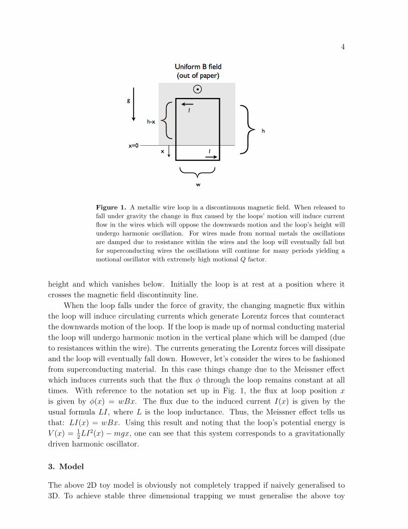
magnetically levitated mechanical system. For this toy model, we consider a wire loop

of superconducting material oriented in a vertical plane (Fig. 1) and threaded by a

discontinuous horizontal magnetic field which is uniform and non-zero above a certain

4

Figure 1. A metallic wire loop in a discontinuous magnetic field. When released to

fall under gravity the change in flux caused by the loops’ motion will induce current

flow in the wires which will oppose the downwards motion and the loop’s height will

undergo harmonic oscillation. For wires made from normal metals the oscillations

are damped due to resistance within the wires and the loop will eventually fall but

for superconducting wires the oscillations will continue for many periods yielding a

motional oscillator with extremely high motional Q factor.

height and which vanishes below. Initially the loop is at rest at a position where it

crosses the magnetic field discontinuity line.

When the loop falls under the force of gravity, the changing magnetic flux within

the loop will induce circulating currents which generate Lorentz forces that counteract

the downwards motion of the loop. If the loop is made up of normal conducting material

the loop will undergo harmonic motion in the vertical plane which will be damped (due

to resistances within the wire). The currents generating the Lorentz forces will dissipate

and the loop will eventually fall down. However, let’s consider the wires to be fashioned

from superconducting material. In this case things change due to the Meissner effect

which induces currents such that the flux φ through the loop remains constant at all

times. With reference to the notation set up in Fig. 1, the flux at loop position x

is given by φ(x) = wBx. The flux due to the induced current I(x) is given by the

usual formula LI, where L is the loop inductance. Thus, the Meissner effect tells us

that: LI(x) = wBx. Using this result and noting that the loop’s potential energy is

V (x) = 12LI2(x) −mgx, one can see that this system corresponds to a gravitationally

driven harmonic oscillator.

3. Model

The above 2D toy model is obviously not completely trapped if naively generalised to

3D. To achieve stable three dimensional trapping we must generalise the above toy

5

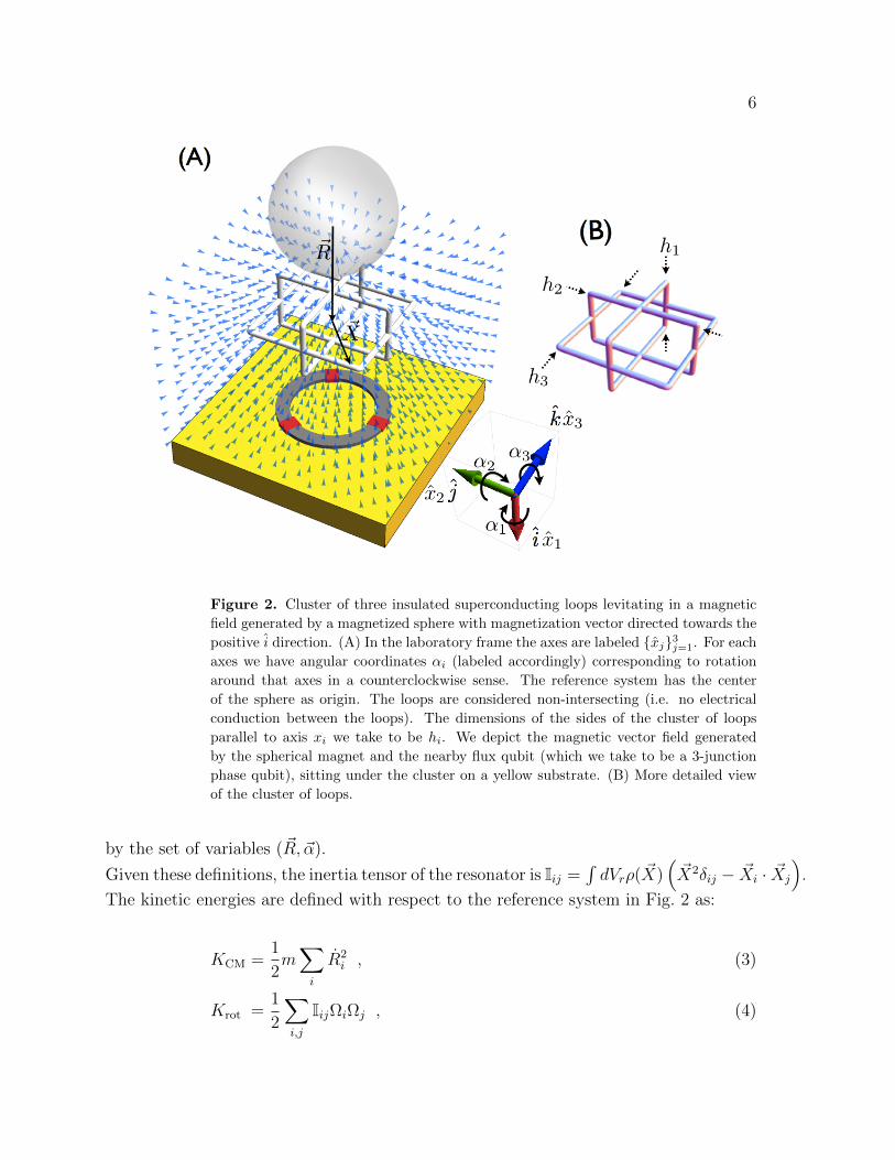
model in a more sophisticated manner. Let us now consider the system sketched in

Fig. 2. We consider a spatially strongly inhomogeneous magnetic field generated by a

fixed magnetized sphere placed above a cluster (the motional resonator) of three non-

intersecting loops oriented along mutually orthogonal planes. This particular shape will

allow the potential energy of the system to have a stable minimum and also leads to

a diagonal inductance matrix, so that the current flowing in one loop does not induce

any currents in the other loops. A flux qubit is placed at a certain distance from the

center of the cluster of loops. The inductive coupling between the flux qubit and the

cluster will provide us with the control required to establish motional cooling of the

levitated cluster. In the following we first study the system classically to establish full

3D trapping, translation/rotation oscillation frequencies at the trap minimum, before

studying the quantum mechanics and motional cooling protocols to cool the vertical

translational degree of freedom towards the ground state.

The total Hamiltonian H is the sum of terms involving the motional resonator (Hr),

the qubit (Hq) and the interaction (HI):

H = Hr +Hq +HI , (1)

and in the following sections we develop each of these individual Hamiltonians.

3.1. Resonator

The Hamiltonian of the cluster of loops (which we will now denote as the motional

resonator or simply resonator), can be written in the following form:

Hr = KCM +Krot + V , (2)

where KCM is the kinetic energy due to the translational motion of the center of

mass, Krot is the rotational kinetic energy and V is the effective potential energy as a

function of the translational and rotational degrees of freedom. We will now define some

notation used in the following.

• m: mass of the resonator.

• ~X: vector position of the various part of the resonator in a co-rotating reference

frame with origin at the center of mass.

• ~R: coordinates of the center of mass in the laboratory reference frame.

• ~r: vector position of the various part of the resonator in the laboratory frame.

• ~r = ~r − ~R

Note that the origin of the laboratory frame is taken to be at the center of the magnetic

sphere (see Fig. 2).

Because of the rigid body properties, the only allowed relation between r( ~X, t) and~X is given by r( ~X, t) = O(t) ~X, where O = e

∑i αi(t)Ti (with (Ti)jk = εijk) is a ro-

tation matrix and αi ∈ [−π, π]. We can then define the angular velocity vectors as:

Ωi = O(t)−1O(t) = αiTi. The motion of the rigid body is thus completely determined

6

Figure 2. Cluster of three insulated superconducting loops levitating in a magnetic

field generated by a magnetized sphere with magnetization vector directed towards the

positive i direction. (A) In the laboratory frame the axes are labeled xj3j=1. For each

axes we have angular coordinates αi (labeled accordingly) corresponding to rotation

around that axes in a counterclockwise sense. The reference system has the center

of the sphere as origin. The loops are considered non-intersecting (i.e. no electrical

conduction between the loops). The dimensions of the sides of the cluster of loops

parallel to axis xi we take to be hi. We depict the magnetic vector field generated

by the spherical magnet and the nearby flux qubit (which we take to be a 3-junction

phase qubit), sitting under the cluster on a yellow substrate. (B) More detailed view

of the cluster of loops.

by the set of variables (~R, ~α).

Given these definitions, the inertia tensor of the resonator is Iij =∫dVrρ( ~X)

(~X2δij − ~Xi · ~Xj

).

The kinetic energies are defined with respect to the reference system in Fig. 2 as:

KCM =1

2m∑i

R2i , (3)

Krot =1

2

∑i,j

IijΩiΩj , (4)

7

The potential V is just the sum of the flux energy due to the current flowing in the

loops and the gravitational potential energy:

V =1

2

3∑a=1

LaI2a −mgR1 , (5)

where the index a = 1, 2, 3 labels the loops accordingly to the direction

perpendicular to the plane of the loop (where 1→ i, 2→ j, 3→ k), La is the inductance

of the loop a and Ia is the current flowing in the loop a. By the symmetry of the resonator

the mutual inductances between the loops is zero. The currents are just functions of the

six degrees of freedom (translations, rotations), describing the motion of the resonator

via equations originating from the Meissner effect:

∆φa(~R, ~α) + LaIa(~R, ~α) = 0 , (6)

where ∆φa(~R, ~α) = φa(~R, ~α)−φa(~R(0), ~α(0)) is the difference in magnetic flux threading

loop a when the system is in the configuration labeled by (~R, ~α) and when the system

is in its initial configuration (~R(0), ~α(0)). Any infinitesimal change in flux due to an

infinitesimal displacement/rotation induces a supercurrent whose action is to restore the

loop’s position/orientation. The stronger this restoring force is the higher the oscillation

frequency will be. We now compute the dependence of the magnetic flux on the system’s

configuration.

We start by calculating the magnetic flux threading the loops. The vector potential~A generated by a sphere with homogeneous magnetization vector ~M calculated at the

point ~r + ~R (where ~R is the center of mass position vector referenced from the centre

of our coordinate system - the centre of the sphere), is just:

~A(~r; ~M, ~R) =µ0

4π

1

|~r + ~R|3~M ∧ (~r + ~R) . (7)

If we denote with ~Σa the area vector of loop a, then the flux through this loop can

be expressed as:

φa(~R, ~α) =

∫Σ

~B · d~Σa =

∫∂Σa

~A · d~r . (8)

In a first order approximation and by supposing that the initial position of the

resonator is such that αi = 0, we have:

∆φa =µ0

4π( ~Ka · [~r − ~R(0) ∧ ~α] + ~Qa · [ ~M ∧ ~α]) , (9)

where the vectors ~Ka and ~Qa are easily calculated from the magnetic field and the sphere

magnetization. By using Eq. (5) and Eq. (6) we can expand the potential energy to

second order in spatial and angular coordinates as:

E =1

2Eijζ

iζj , (10)

8

where ~ζ = x, y, z, αx, αy, αz, is a vector whose components are all the parameters

describing the motion and where the matrix elements Eij depend on the vectors defined

just above.

In Section 5 we will show how certain choices of the parameters of our system can

lead to a decoupled degree of freedom (the vertical direction with associated variable

R1), with a quite high oscillating frequency ωr. This frequency is also well resolved

with respect to the frequencies of the other modes (the difference between frequencies

is bigger than the linewidth of the resonator), hence it can be well resolved by the qubit

coupling. Note however, that this mode is strictly decoupled from other rotational and

motional modes only to second order in perturbation theory hence it is important that

the system be initialized not too far from equilibrium. We will consider the quantized

variable corresponding to small deviations from the initial position along the i axis:

x ≡ R1 − x0 (x0 being the x component of the vector ~R0), whose quantum operator we

define as:

x = (

√~

2mωr)(a+ a†) . (11)

The dynamics of this variable is governed by an harmonic Hamiltonian whose frequency

ωr can be obtained through the energy given above in Eq. (10).

3.2. Qubit

The flux qubit is considered to have characteristic frequency ωq and to be driven by

a classical field of frequency ωd slightly detuned by ωq. The detuning parameter is

δ = ωd−ωq. The field drives the qubit with Rabi frequency Ω. The Hamiltonian in the

rotating frame with frequency ωd is:

Hq = −δ2σz +

Ω

2σx . (12)

3.3. Interaction

The classical interaction Hamiltonian for the inductive coupling between the loops of

the cluster and the loop of the flux qubit is given by:

HI = MrqIrIq , (13)

where Mrq is the mutual inductance between the qubit and the loop of the resonator

which is horizontal in the initial position and Ir = I1 and Iq are the currents flowing

in that loop and in the qubit. Because we are considering small deviations from the

equilibrium initial position, we neglect the mutual interactions between the other loops

or due to the angular motion of the object. We will consider the dependence of the

coupling in the vertical direction by performing a first order expansion. We expand Irto first order in small deviations from the initial position using (9). In the quantized

9

version we also replace Iq with Iqσz (see for example [25]). Denoting DI(0) = ∂Ir∂x

∣∣∣~R(0)

as

the derivative of the current evaluated at the initial cluster position and remembering

(11) we write the quantized interaction Hamiltonian as:

HI = ~λ

2(a+ a†)σz , (14)

with:

λ =

(√2

m~ωr

)MDIl(0)Iq . (15)

The mutual inductance is simply calculated as:

M =µ0

4π

∫d~sd~s ′

R, (16)

where d~s and d~s′ are vectors tangent to the two loops and R is the distance between

the infinitesimal part of each loop and the integration is along each of the two loops.

The final quantized expression for the Hamiltonian describing the motion of the

cluster in the vertical direction and its interaction with the qubit is (setting ~ = 1):

H = −δ2σz +

Ω

2σx + ωra

†a+λ

2(a+ a†)σz . (17)

In order to be in the motional quantum regime we must devise cooling schemes to bring

the resonator close to its motional ground state as described in the next section.

4. Cooling

4.1. Cooling scheme A: Introduction

Following [26] we will consider the resonator and the qubit coupled to separate thermal

baths and interacting with each through the coupling HI (see Fig. 3).

The system’s quantum motional state, ρ evolves under the following master

equation:

˙ρ = −i[H, ρ] + LΓ(ρ) + Lγ(ρ) . (18)

The qubit Liouville operator contains decay and dephasing with rates Γ⊥ and Γ||:

LΓ(ρ) =Γ⊥2

(Nq + 1)(2σ−ρσ+ − σ+σ−ρ− ρσ+σ−) +

+Γ⊥2

(Nq)(2σ+ρσ− − σ−σ+ρ− ρσ−σ+) +

+Γ||2

(σzρσz − ρ) , (19)

10

where Nq = (e~ωqkBT − 1)−1, and where T is the temperature of the qubit bath. The

Lioville operator for the motional resonator is:

Lγ(ρ) =γ

2(Nth + 1)(2aρa† − a†aρ− ρa†a) +

+γ

2(Nth)(2a

†ρa− aa†ρ− ρaa†) , (20)

where the mechanical dissipation factor γ has been introduced, and the equilibrium

phonon occupation number is Nth = (e~ωrkBT − 1)−1.

We now trace out the qubit to find an effective equation of motion for the resonator.

From this we will see that under certain cases we can obtain a motional cooling process

bringing the cluster towards its motional ground state. We will consider the two different

temperature regimes studied in [26].

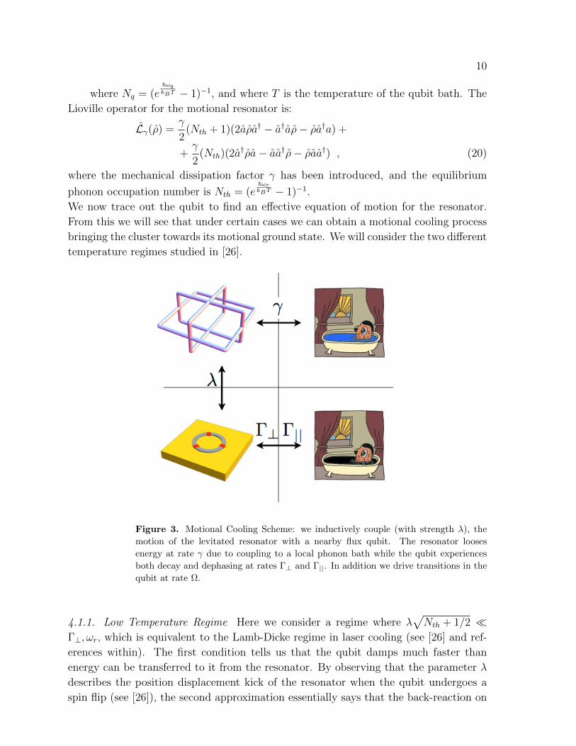
Figure 3. Motional Cooling Scheme: we inductively couple (with strength λ), the

motion of the levitated resonator with a nearby flux qubit. The resonator looses

energy at rate γ due to coupling to a local phonon bath while the qubit experiences

both decay and dephasing at rates Γ⊥ and Γ||. In addition we drive transitions in the

qubit at rate Ω.

4.1.1. Low Temperature Regime Here we consider a regime where λ√Nth + 1/2

Γ⊥, ωr, which is equivalent to the Lamb-Dicke regime in laser cooling (see [26] and ref-

erences within). The first condition tells us that the qubit damps much faster than

energy can be transferred to it from the resonator. By observing that the parameter λ

describes the position displacement kick of the resonator when the qubit undergoes a

spin flip (see [26]), the second approximation essentially says that the back-reaction on

11

the resonator following a qubit flip is small relative to the oscillator energy.

Thanks to these assumptions one can write the full density matrix as ρ(t) 'ρ0q ⊗ ρr(t) where ρ0

q is the qubit steady state density matrix. In this way one can obtain

an effective master equation for the resonator after having traced out the qubit. The

result can be encoded in a new effective mechanical damping factor given by Γ = ΓC +γ

with ΓC = S(ωr)− S(−ωr) where S(ω) denotes the qubit fluctuation spectrum:

S(ω) =λ2

2Re

∫ ∞0

eiωτ dτ〈σz(τ)σz(0)〉0 − 〈σz〉20

, (21)

and where 〈·〉0 denotes the steady state expectation [26]. What interests us is the

final motional occupation number which is given by:

nLD =γNth

ΓC+N0 , (22)

where N0 = S(−ωr)/ΓC , and the subscript stresses the Lamb-Dicke regime we are

supposing.

4.1.2. High Temperature Regime As one can see from (22), for low enough Nth the final

occupation number is given by N0. Increasing the temperature of the motional bath we

see that the final occupation number grows linearly with Nth. However, when Nth is

so large the previous assumptions λ√Nth + 1/2 Γ⊥, ωr do not hold true anymore it

turns out [26] that, under the temperature independent assumptions (λ Γ⊥, ωr), one

can study situations in which the final occupation number is given by the more general

formula:

nf = Nth

(ζ +

1− ζ1 + ζeI1/(Nthζη2)

), (23)

with parameters defined in Appendix A. As described in that section, in order to obtain

this formula one must consider the resonator‘s initial quantum state is given by the

coherent state |α〉〈α| with |α|2 ∼ Nth a coherent state labeled by the parameter α as

initial condition. Given this assumption the “renormalized” cooling rate ΓC is an α

dependent quantity.

4.2. Cooling scheme B

Rather than use the scheme depicted in Fig 3, one can also cool the motion of the

resonator (at least in the case of near resonance with the qubit) by performing a sequence

of repeated measurements on the flux qubit inductively coupled to the resonator’s

position [27].

Using a flux qubit made out of three superconducting loops with four Josephson

junctions one [28, 29] can tune the magnetic energy bias ~δ to zero. We also assume

that the inductive coupling strength is much smaller than the qubit frequency (λ ωr).

This will allow us to perform a rotating wave approximation on the Hamiltonian of the

12

full system. We consider the system to be initially prepared in the separable state

ρ0 = |g〉〈g|⊗ρr with the resonator in the thermal state ρnr = 〈n|ρr|n〉 = e−nβ~ωr

1−e−β~ωr . Then,

one performs N measurements on the qubit (with associated operator given by |g〉〈g|and |e〉〈e| where g (e) is the ground (excited) state) at times tj = jτ where τ is short

time interval. One finds that, provided the measurement outcome is always |g〉〈g|, at

the conclusion of these N measurements the state of the resonator is [27]:

ρr(N) =∑n≥0

|µn|2Nρnr |n〉〈n|P (N)

, (24)

where µ0 = ei∆τ/2, µn = e−i(n−1/2)ωrτ (cos Ωnτ + i sin Ωnτ cos 2θn), Ωn =√(∆− ωr)2/4 + g2n (n ≥ 1), tan 2θn = 2g

√n/(∆−ωn) (n ≥ 1) and where N indicates

the number of measurements. P (N) is the probability this sequence of measurement

outcomes occurs.

5. Results

Here we consider our 3D model in a more realistic setting and adopt physical parameters

in the table shown in section 8. Using this physically realistic set of parameters we now

examine in more concrete detail the classical and quantum mechanics of the resonator

and the levels of cooling achieved by the above outlined methods.

5.1. Classical Motion

We now examine the classical motion of the resonator by focusing in particular on its

stability and its frequency of oscillation.

The effect of the gravity in the potential energy V (x) causes a small and negligible shift

of the potential minimum.

By considering the magnetization of the sphere to be aligned along the vertical x direc-

tion and expanding to second order the potential energy around its minimum, one finds

that the x-motion decouples from the other directions. One finds further the existence

of three degrees of freedom which are “zero modes”, i.e. do not contribute to the energy

up to third order. One zero-mode is related to the rotational symmetry around the

vertical axes. The other two are due to the coupling between the variables y(z) and

αz(αy). however, if one considers these contributions to higher orders these degrees of

freedom contribute to the energy value to give overall stability as shown in Fig. 5. For a

cluster of loops of ”typical “dimensions (as defined below) of (1, 10, 10) µm and with a

wire thickness of 0.1 µm the root mean square thermal motion of the cluster at 15 mK

is ∼ 10−12 m along the spatial directions and 10−6 radians along the αy and αz angular

directions (while there is symmetry along the other angular direction).

The frequency of the translational motions depends on the physical dimensions of

the cluster of loops. In Fig. 6 the frequency in the x and y-direction is plotted as a

13

Figure 4. Exact numerical evaluation of the potential energy (in units of E0 = ~ωr)

as a function of the vertical translational degree of freedom x (with origin the stable

point and in unit of x0 =√

~mωr

).

Figure 5. Exact numerical evaluation of the potential energy as a function of the

horizontal translational degree of freedom y (with origin the stable point) and the

angular degree of freedom αz. Because the potential is confining to third order in

these degrees of freedom the overall system is stable.

function of a scaling factor k for the system. The values for all the parameters are

explicitly shown in the table in section 8.

The frequencies decrease as the scaling grows, showing that the trapping in the transla-

tional degrees of freedom is becoming less tight, but still present for a large range of size

scales. In regards of the rotational degrees of freedom, even when the system is scaled

up with a factor 10 with respect to the typical parameters, numerically we find that the

trapping is still achieved in the small oscillation regime (see section 3.1).

In summary, using the parameters shown the table in section 8, for small loops

and very high magnetic field inhomogeneities the cluster of loops experiences stable,

levitated magnetic trapping. The frequency of oscillation along the x-direction is larger

than in the other directions making it easier to cool. For these reasons, in the following

we quantize the x-translational motion.

14

Figure 6. Translational mode frequency as a function of system size. The frequency

along the x direction (blue line) and y (and for symmetry reasons z) direction (red

line) are plotted as a function of the scaling factor k which defines the dimension of

the system. The radius of the magnetized sphere is defined as Rsp = k µm. The

dimension of the parallelepiped enveloping the cluster of loops is k× (0.1, 1, 1)µm and

the thickness of the wires is k × 0.01 µm. The cluster mass scales as k3. When

considering different values for the scale factor, the initial position of the center of

the cluster of loops is chosen to keep the distance between the center of the sphere to

the top of the cluster fixed at ∼ 1.1 Rsp where Rsp is the radius of the sphere. The

frequencies are higher for smaller sizes of the system. As “typical” parameters for the

system we will consider the ones given by a scaling factor k = 10.

5.2. Superconductivity and Dissipation

The superconducting loops are considered as made out of Niobium-Tin (NbSn) which, in

normal conditions, has very high critical magnetic field strength (∼ 30 T ), although, in

our case, the situation is more critical due to the small thickness of the superconducting

wires.

We now examine two types of motional decay mechanisms and estimate the resulting

motional Q for the resonator‘s motion. We first consider the loss in energy from the

moving resonator due to its action as a dipole emitter of radiation.

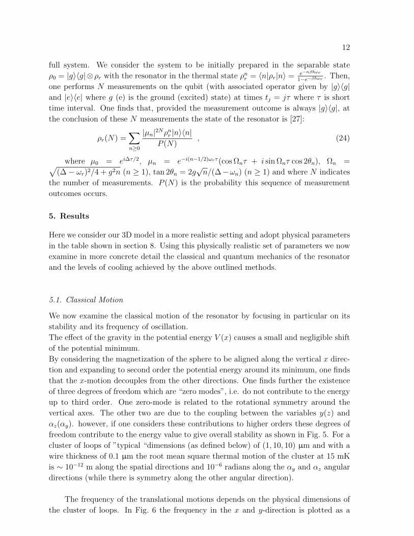
In Fig. 7 the intensity of the magnetic field (in Tesla) is plotted as a function of distance

from the center of the magnetized sphere (radius 10µ m).

As we saw above, the motion of the cluster of loops is trapped in all three directions.

Due to the Messnier effect, the greater the spatial excursion from its equilibrium position

the greater the current density inside the wires. Considering the physical parameters

given in the table in section 8 we find typical current densities of ∼ (108, 108, 107)A/m2

(respectively in the loops perpendicular to the x, y, z directions).Considering each

current to be described by I = I0e−iωt, where ω is the top frequency in each direction,

by approximating the loops to be circular we can calculate the power dissipated by the

15

Figure 7. Magnetic field intensity along the vertical x.

oscillating currents as electromagnetic radiation as (see for example [30]):

Prad =1

2

π

6

4π

c

2πr

λ

I0

2, (25)

where r is the radius of the loop and λ = c/ν (where c is the speed of light). From

this we observe that the power radiated is absolutely negligible.

However, the main source of dissipation is the viscous drag of flux lines oscillating inside

the pinning wells inside the superconducting wires [7]. One can estimate the motional

quality factor Q = ωrγ

for a system similar to (the two dimensional version of) the one

presented here to be Q ≈ 1011. In our calculations we will consider Q ≈ 1010. Such

an enormously high motional quality factor is already known in levitating systems [31]

(Q ∼ 1012), although typically one finds motional Q values in the range ∼ 103/106 for

cavity optomechanical experiments [22]. The prospect for ultra-large motional Q is one

of the primary benefits of our scheme.

5.3. Coupling between the resonator and the flux qubit.

In this section we will study the coupling between the resonator and the flux qubit. The

possibility to tune this coupling arises from the (distance dependent) inductive nature

of the coupling.

Fig. 8 shows the value of the coupling strength between the qubit and the resonator as

a function of the distance d between the center of mass of the resonator and the center

of the loop of the flux qubit the latter taken to be a circle of radius 5µm.

We observe that the coupling strength can be adjusted over quite a large range by

fixing the distance between the qubit and the resonator.

5.4. Cooling of the motional resonator.

5.4.1. Cooling scheme A. In this cooling scheme the motional energy of the resonator

is damped away thanks to the faster decay of the flux qubit.

We will start by studying the low temperature limit. This means that the Nth of the

16

Figure 8. Coupling constant between the qubit and the resonator. The coupling arise

from the mutual inductance between the loops of the resonator and the qubit loop.

By supposing the loop of the qubit to be placed in a plance orthogonal to the vertical

direction, the contribution to the coupling comes, in a good approximation, from the

loop of the resonator perpendicular to the x direction. The distance d is defined as the

distance between the center of mass of the resonator and the center of the qubit loop.

The qubit loop is supposed to have a 5µm long radius.

bath connected to the resonator must be such that λ√Nth + 1

2 Γ⊥, ωr is fulfilled.

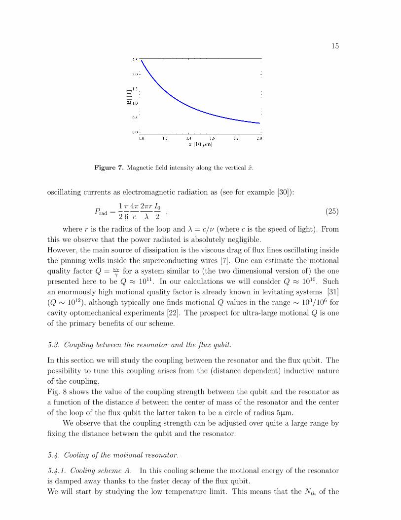
In Fig. 9 we plot the final motional average Fock number as a function of the qubit

resonance frequency ωq and Rabi frequency Ω, while in Fig. 10 we plot the same final

occupation number as a function of ωq after fixing Ω to an optimal value. In particular,

we chose the Rabi frequency Ω and the detuning δ to fulfill the relation ωq =√

Ω2 + δ2.

For comparison, the dashed line in Fig. 9 shows the equilibrium phonon number if the

resonator is in equilibrium with a 15 mK thermal bath. The cooling happens in the

region defined by the dashed line. Fig. 10, which is a section of Fig. 9 obtained by fixing

Ω.

Now we move to a regime where no constraints on the temperature of the bath

connected to the resonator are imposed so that the only relations to be fulfilled are

λ Γ⊥, ωr. This will allow us to use an higher coupling constant with respect to the

low (but still non-zero) temperature limit, previously considered.

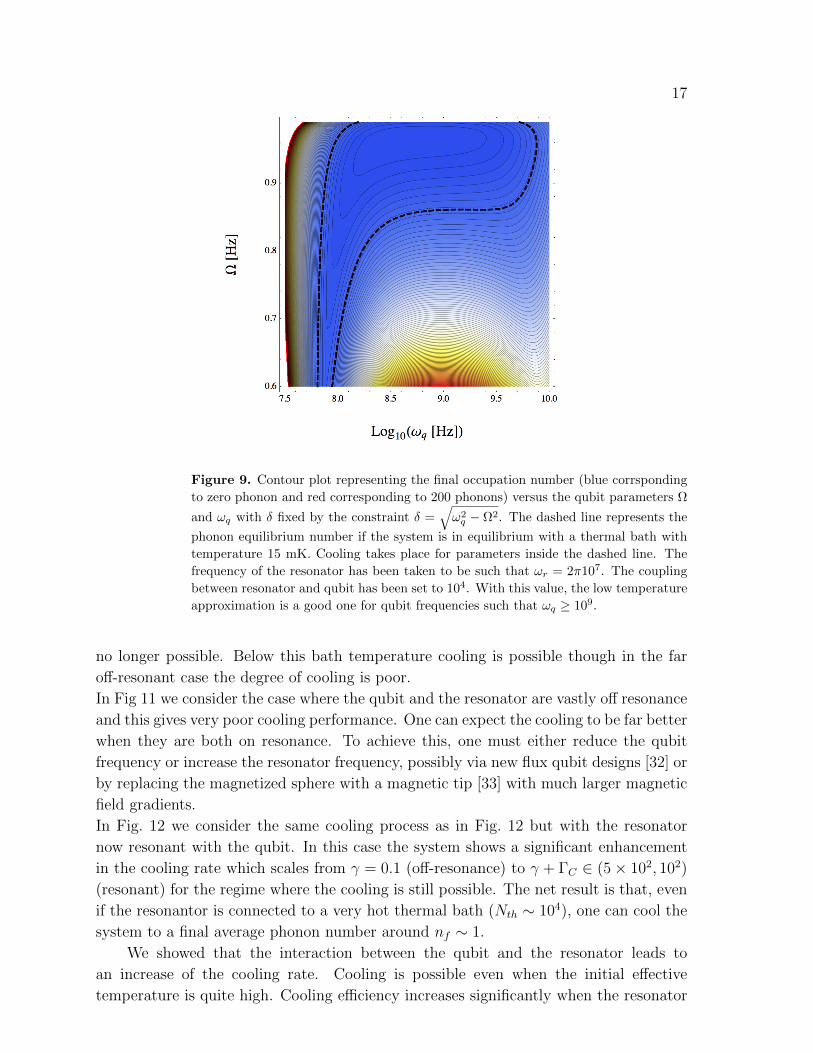
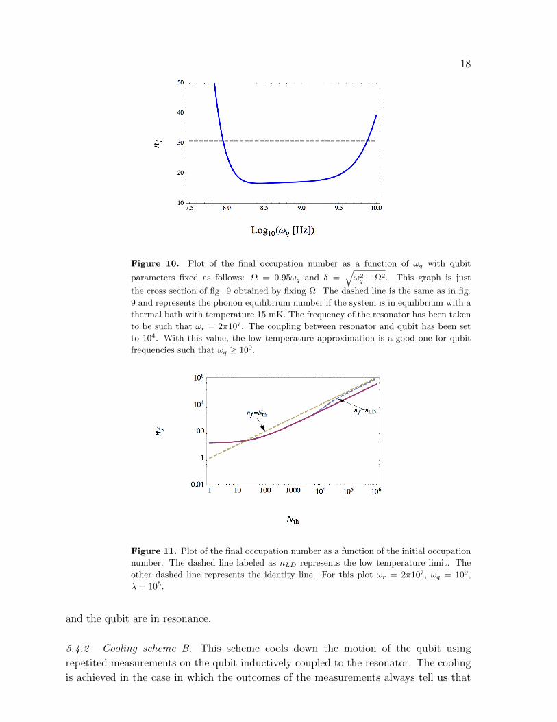
Fig. 11 shows the final expected cooled final motional Fock number nr in the case where

there exist a large frequency mismatch between the qubit and the resonator. As expected

the cooling is quite poor. For comparison, we also plot the dashed line labeled as nLDobtained from the low temperature theory extrapolated to high temperature (as given

by Eq. (22)). One can see that in the low temperature regime the two theories agree

while at high temperatures they disagree. Above a certain bath temperature cooling is

17

Figure 9. Contour plot representing the final occupation number (blue corrsponding

to zero phonon and red corresponding to 200 phonons) versus the qubit parameters Ω

and ωq with δ fixed by the constraint δ =√ω2q − Ω2. The dashed line represents the

phonon equilibrium number if the system is in equilibrium with a thermal bath with

temperature 15 mK. Cooling takes place for parameters inside the dashed line. The

frequency of the resonator has been taken to be such that ωr = 2π107. The coupling

between resonator and qubit has been set to 104. With this value, the low temperature

approximation is a good one for qubit frequencies such that ωq ≥ 109.

no longer possible. Below this bath temperature cooling is possible though in the far

off-resonant case the degree of cooling is poor.

In Fig 11 we consider the case where the qubit and the resonator are vastly off resonance

and this gives very poor cooling performance. One can expect the cooling to be far better

when they are both on resonance. To achieve this, one must either reduce the qubit

frequency or increase the resonator frequency, possibly via new flux qubit designs [32] or

by replacing the magnetized sphere with a magnetic tip [33] with much larger magnetic

field gradients.

In Fig. 12 we consider the same cooling process as in Fig. 12 but with the resonator

now resonant with the qubit. In this case the system shows a significant enhancement

in the cooling rate which scales from γ = 0.1 (off-resonance) to γ + ΓC ∈ (5× 102, 102)

(resonant) for the regime where the cooling is still possible. The net result is that, even

if the resonantor is connected to a very hot thermal bath (Nth ∼ 104), one can cool the

system to a final average phonon number around nf ∼ 1.

We showed that the interaction between the qubit and the resonator leads to

an increase of the cooling rate. Cooling is possible even when the initial effective

temperature is quite high. Cooling efficiency increases significantly when the resonator

18

Figure 10. Plot of the final occupation number as a function of ωq with qubit

parameters fixed as follows: Ω = 0.95ωq and δ =√ω2q − Ω2. This graph is just

the cross section of fig. 9 obtained by fixing Ω. The dashed line is the same as in fig.

9 and represents the phonon equilibrium number if the system is in equilibrium with a

thermal bath with temperature 15 mK. The frequency of the resonator has been taken

to be such that ωr = 2π107. The coupling between resonator and qubit has been set

to 104. With this value, the low temperature approximation is a good one for qubit

frequencies such that ωq ≥ 109.

Figure 11. Plot of the final occupation number as a function of the initial occupation

number. The dashed line labeled as nLD represents the low temperature limit. The

other dashed line represents the identity line. For this plot ωr = 2π107, ωq = 109,

λ = 105.

and the qubit are in resonance.

5.4.2. Cooling scheme B. This scheme cools down the motion of the qubit using

repetited measurements on the qubit inductively coupled to the resonator. The cooling

is achieved in the case in which the outcomes of the measurements always tell us that

19

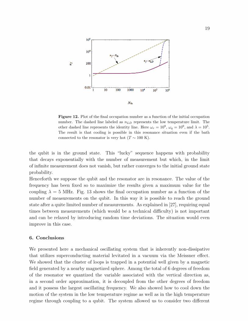
Figure 12. Plot of the final occupation number as a function of the initial occupation

number. The dashed line labeled as nLD represents the low temperature limit. The

other dashed line represents the identity line. Here ωr = 109, ωq = 109, and λ = 105.

The result is that cooling is possible in this resonance situation even if the bath

connected to the resonator is very hot (T ∼ 100 K).

the qubit is in the ground state. This “lucky” sequence happens with probability

that decays exponentially with the number of measurement but which, in the limit

of infinite measurement does not vanish, but rather converges to the initial ground state

probability.

Henceforth we suppose the qubit and the resonator are in resonance. The value of the

frequency has been fixed so to maximize the results given a maximum value for the

coupling λ = 5 MHz. Fig. 13 shows the final occupation number as a function of the

number of measurements on the qubit. In this way it is possible to reach the ground

state after a quite limited number of measurements. As explained in [27], requiring equal

times between measurements (which would be a technical difficulty) is not important

and can be relaxed by introducing random time deviations. The situation would even

improve in this case.

6. Conclusions

We presented here a mechanical oscillating system that is inherently non-dissipative

that utilizes superconducting material levitated in a vacuum via the Meissner effect.

We showed that the cluster of loops is trapped in a potential well given by a magnetic

field generated by a nearby magnetized sphere. Among the total of 6 degrees of freedom

of the resonator we quantized the variable associated with the vertical direction as,

in a second order approximation, it is decoupled from the other degrees of freedom

and it possess the largest oscillating frequency. We also showed how to cool down the

motion of the system in the low temperature regime as well as in the high temperature

regime through coupling to a qubit. The system allowed us to consider two different

20

Figure 13. Plot about the cooling by mean of measurements on the qubit. The blue

line represents the plot of the final occupation number nf as a function of the number

of measurements on the qubit. The red line represents the survival probabilty P (N)

which, for N → ∞, goes to the initial probability to find the system in the ground

state. For this plot the resonator is interacting with a T = 15mK thermal bath and

we consider a resonant situation with ωr = ωq = 2.5 × 108 Hz, λ = 5 × 106 Hz and

τ = 10ωr

s.

cooling schemes which work very well in the case resonator and qubit are resonant. The

system can be improved by considering stronger or higher gradient magnetic fields, which

could be achieved by replacing the magnetized sphere with other geometric magnetized

objects. This is not the only direction for further studies. In fact a complete analysis

would quantize all the degrees of freedom and would find a way to cool all of them (for

example by introducing other inductive couplings with other flux qubit).

7. Acknowledgements

We thank Gerald Milburn for many helpful comments and discussions. This research

was supported by the ARC via the Centre of Excellence in Engineered Quantum Systems

(EQuS), project number CE110001013.

21

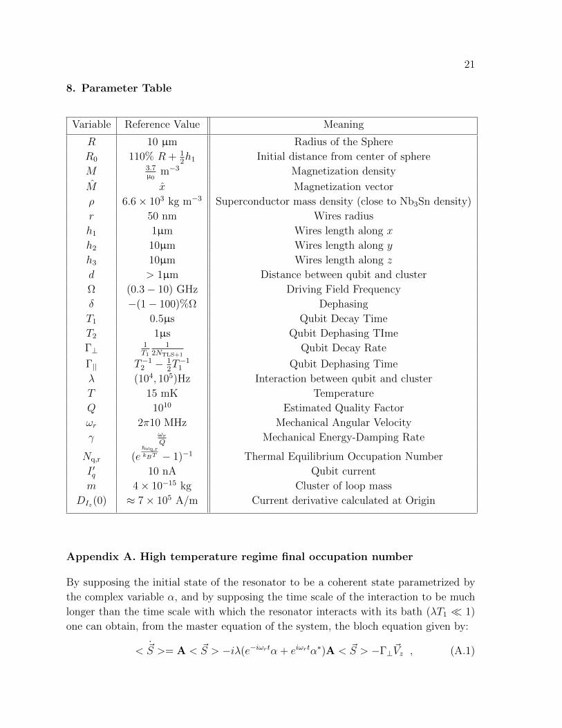
8. Parameter Table

Variable Reference Value Meaning

R 10 µm Radius of the Sphere

R0 110% R + 12h1 Initial distance from center of sphere

M 3.7µ0

m−3 Magnetization density

M x Magnetization vector

ρ 6.6× 103 kg m−3 Superconductor mass density (close to Nb3Sn density)

r 50 nm Wires radius

h1 1µm Wires length along x

h2 10µm Wires length along y

h3 10µm Wires length along z

d > 1µm Distance between qubit and cluster

Ω (0.3− 10) GHz Driving Field Frequency

δ −(1− 100)%Ω Dephasing

T1 0.5µs Qubit Decay Time

T2 1µs Qubit Dephasing TIme

Γ⊥1T1

12NTLS+1

Qubit Decay Rate

Γ|| T−12 − 1

2T−1

1 Qubit Dephasing Time

λ (104, 105)Hz Interaction between qubit and cluster

T 15 mK Temperature

Q 1010 Estimated Quality Factor

ωr 2π10 MHz Mechanical Angular Velocity

γ ωrQ

Mechanical Energy-Damping Rate

Nq,r (e~ωq,rkBT − 1)−1 Thermal Equilibrium Occupation Number

I ′q 10 nA Qubit current

m 4× 10−15 kg Cluster of loop mass

DIz(0) ≈ 7× 105 A/m Current derivative calculated at Origin

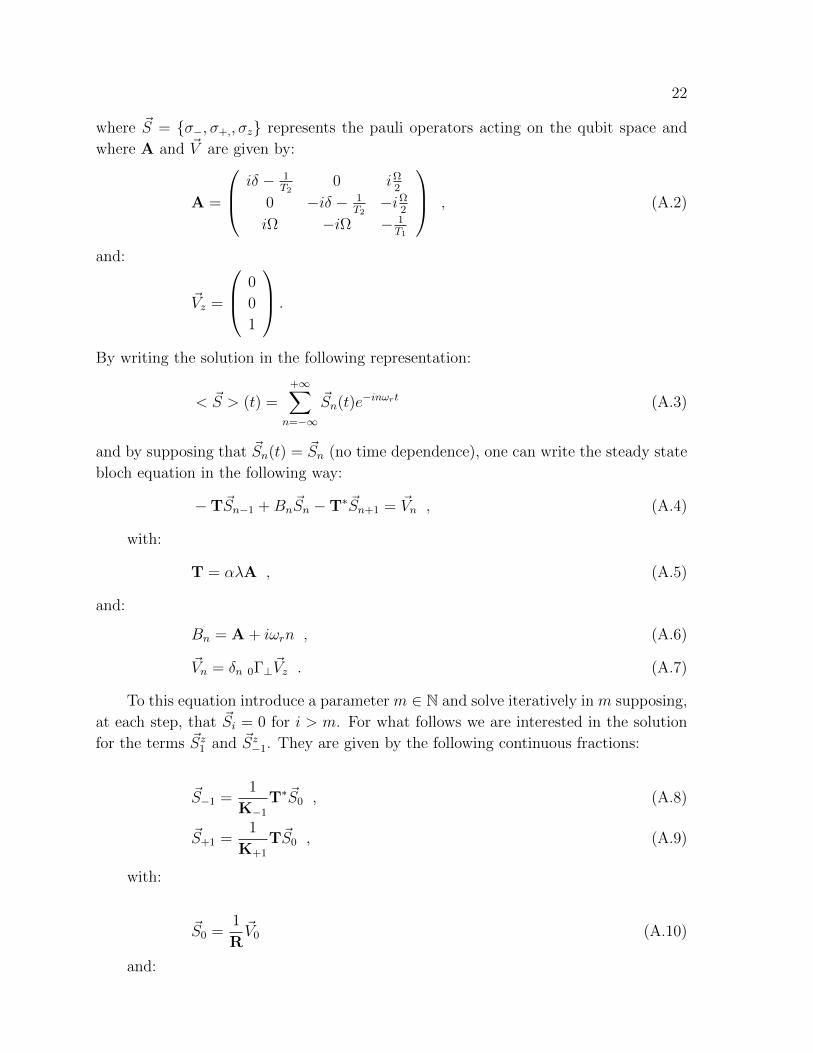
Appendix A. High temperature regime final occupation number

By supposing the initial state of the resonator to be a coherent state parametrized by

the complex variable α, and by supposing the time scale of the interaction to be much

longer than the time scale with which the resonator interacts with its bath (λT1 1)

one can obtain, from the master equation of the system, the bloch equation given by:

< ~S >= A < ~S > −iλ(e−iωrtα + eiωrtα∗)A < ~S > −Γ⊥~Vz , (A.1)

22

where ~S = σ−, σ+,, σz represents the pauli operators acting on the qubit space and

where A and ~V are given by:

A =

iδ − 1T2

0 iΩ2

0 −iδ − 1T2−iΩ

2

iΩ −iΩ − 1T1

, (A.2)

and:

~Vz =

0

0

1

.

By writing the solution in the following representation:

< ~S > (t) =+∞∑

n=−∞

~Sn(t)e−inωrt (A.3)

and by supposing that ~Sn(t) = ~Sn (no time dependence), one can write the steady state

bloch equation in the following way:

−T~Sn−1 +Bn~Sn −T∗~Sn+1 = ~Vn , (A.4)

with:

T = αλA , (A.5)

and:

Bn = A + iωrn , (A.6)

~Vn = δn 0Γ⊥~Vz . (A.7)

To this equation introduce a parameter m ∈ N and solve iteratively in m supposing,

at each step, that ~Si = 0 for i > m. For what follows we are interested in the solution

for the terms ~Sz1 and ~Sz−1. They are given by the following continuous fractions:

~S−1 =1

K−1

T∗~S0 , (A.8)

~S+1 =1

K+1

T~S0 , (A.9)

with:

~S0 =1

R~V0 (A.10)

and:

23

K−1 = −T1

· |−2

T∗ +B−1 , (A.11)

K+1 = −T∗1

·∗ |+2

T +B+1 , (A.12)

R = K−1 +B0 + K+1 , (A.13)

where · and ·∗ are defined recursively as:

·|−2 = −T1

· |−3

T∗ +B−2 , (A.14)

·∗|+2 = −T∗1

·∗ |+3

T +B+2 . (A.15)

One can stop after a certain amount of iteration by simply substituting, instead of

the previous recursive relation, the ending one:

·|−n = B−n , (A.16)

·∗|+n = B+n . (A.17)

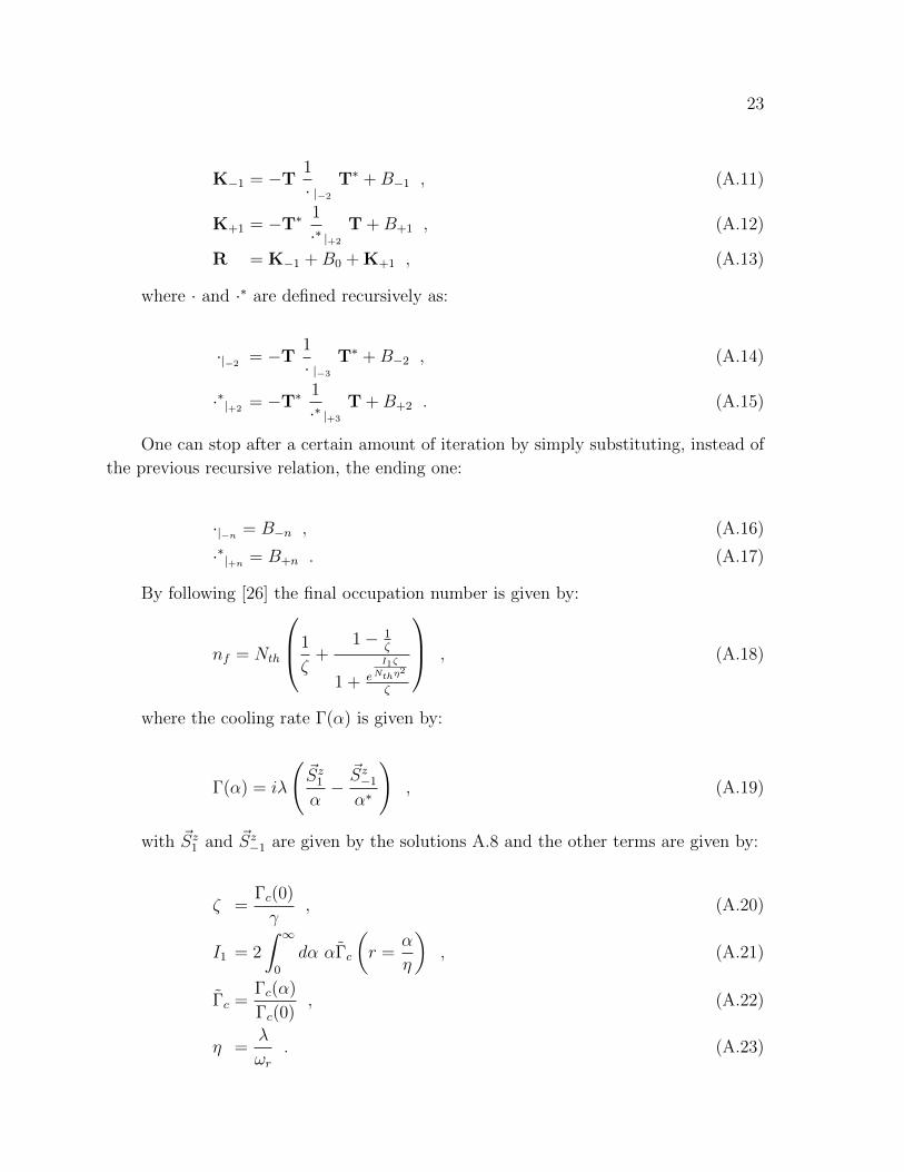
By following [26] the final occupation number is given by:

nf = Nth

1

ζ+

1− 1ζ

1 + e

I1ζ

Nthη2

ζ

, (A.18)

where the cooling rate Γ(α) is given by:

Γ(α) = iλ

(~Sz1α−~Sz−1

α∗

), (A.19)

with ~Sz1 and ~Sz−1 are given by the solutions A.8 and the other terms are given by:

ζ =Γc(0)

γ, (A.20)

I1 = 2

∫ ∞0

dα αΓc

(r =

α

η

), (A.21)

Γc =Γc(α)

Γc(0), (A.22)

η =λ

ωr. (A.23)

24

References

[1] Bustamante C, Chemla Y, Forde N and Izhaky D 2004 Annu. Rev. Biochem. 73 705–748 ISSN

0066-4154

[2] Friedsam C, Wehle A K, Khner F and Gaub H E 2003 J. Phys.-Condens. Mat. 15 S1709

[3] Benoit M G H 2002 Cells Tissues Organs 172 174

[4] Rugar D, Budakian R, Mamin H J and Chui B W 2004 Nature 430 329–332

[5] K L Ekinci Y T Yang M L R 2004 J. Appl. Phys. 95

[6] Burns D, Zook J, Horning R, Herb W and Guckel H 1995 Sensor. actuat. A-Phys. 48 179 – 186

ISSN 0924-4247

[7] Schilling O F 2007 Braz. J. Phys. 37(2A) 425–428

[8] Cleland A N and Roukes M L 1998 Nature 392 160–162

[9] Bocko M F and Onofrio R 1996 Rev. Mod. Phys. 68 755–799

[10] Nakamura Y, Pashkin Y A and Tsai J S 1999 Nature 398 786–788

[11] Brune M, Hagley E, Dreyer J, Maıtre X, Maali A, Wunderlich C, Raimond J M and Haroche S

1996 Phys. Rev. Lett. 77 4887–4890

[12] Clarke J, Cleland A N, Devoret M H, Esteve D and Martinis J M 1988 Science 239 992–997

[13] Silvestrini P, Palmieri V G, Ruggiero B and Russo M 1997 Phys. Rev. Lett. 79 3046–3049

[14] Kleckner D and Bouwmeester D 2006 Nature 444 75–78

[15] Arcizet O, Cohadon P F, Briant T, Pinard M and Heidmann A 2006 Nature 444 71–74

[16] Gigan S, Bohm H R, Paternostro M, Blaser F, Langer G, Hertzberg J B, Schwab K C, Bauerle D,

Aspelmeyer M and Zeilinger A 2006 Nature 444 67–70

[17] Kippenberg T J, Rokhsari H, Carmon T, Scherer A and Vahala K J 2005 Physical Review Letters

95 033901

[18] Schliesser A, Del’Haye P, Nooshi N, Vahala K J and Kippenberg T J 2006 Physical Review Letters

97 243905

[19] Thompson J D, Zwickl B M, Yarich A M, Marquardt F, Girvin S M and Harris J 2007

arXiv:0707.1724

[20] Corbitt Tand Chen Y B, Innerhofer E, Muller-Ebhardt H, Ottaway D, Rehbein H, Sigg D,

Whitcomb S, Wipf C and Mavalvala N 2007 Physical Review Letters 98 150802

[21] Chang D E, Regal C A, Papp S B, Wilson D J, Ye J, Painter O, Kimble H J and Zoller P 2010

Proceedings of the National Academy of Sciences 107 1005–1010

[22] Kippenberg T J and Vahala K J 2007 Opt. Express 15 17172–17205

[23] O’Connell A D, Hofheinz M, Ansmann M, Bialczak R C, Lenander M, Lucero E, Neeley M, Sank

D, Wang H, Weides M, Wenner J, Martinis J M and Cleland A N 2010 Nature 464 697–703

[24] Romer R H 1990 Eur. J. Phys. 11 103

[25] Jaehne K, Hammerer K and Wallquist M 2008 New J. Phys. 10 095019

[26] Rabl P 2010 Phys. Rev. B 82 165320

[27] Li Y, Wu L A, Wang Y D and Yang L P 2011 arXiv:1103.4197

[28] Paauw F G, Fedorov A, Harmans C J P M and Mooij J E 2009 Phys. Rev. Lett. 102(9) 090501

URL http://link.aps.org/doi/10.1103/PhysRevLett.102.090501

[29] Fedorov A, Feofanov A K, Macha P, Forn-D P, Harmans C J P M and Mooij J E 2010 Phys. Rev.

Lett. 105(6) 060503 URL http://link.aps.org/doi/10.1103/PhysRevLett.105.060503

[30] McDonald K T 2010 Fitzgerald’s calculation of the radiation of an oscillating magnetic dipole URL

http://www.physics.princeton.edu/~mcdonald/examples/fitzgerald.pdf

[31] Chang D E, Regal C A, Papp S B, Wilson D J, Ye J, Painter O, Kimble H J and Zoller P 2010

PNAS 107 1005–1010

[32] Gustavsson S 2011 arXiv:1104.5212v2

[33] Mamin H J, Poggio M, Degen C L and Rugar D 2007 Nature 2 301–306