Embed Size (px)
Citation preview
MAGNETIC RESONANCE IMAGING AND SPECTROSCOPYFOR THE STUDY OF TRANSLATIONAL DIFFUSION:
APPLICATIONS TO NERVOUS TISSUE
By
ELIZABETH L. BOSSART
A DISSERTATION PRESENTED TO THE GRADUATE SCHOOLOF THE UNIVERSITY OF FLORIDA IN PARTIAL FULFILLMENT
OF THE REQUIREMENTS FOR THE DEGREE OFDOCTOR OF PHILOSOPHY
UNIVERSITY OF FLORIDA
1999

For Juan
iii
ACKNOWLEDGMENTS
The work in this thesis could not have been accomplished without the help of a
great many people – it is truly a collaborative effort. First and foremost, I would like to
thank Dr. Tom Mareci for his help, time and patience over the last few years. Working
with him, I learned a lot about research, and a lot about myself. I would also like to thank
Dr. Steve Blackband for all his counsel and support. Among other things both scientific
and personal, through him I learned when to relax. I would also like to thank Dr.
Raymond Andrew for his encouraging words and advise throughout my graduate career.
His kind words always made me smile.
I would like to thank several people in the lab and around the Brain Institute for
their help in my endeavors. I would like to acknowledge Ron Smith in the Neurosurgery
department of the UF Brain Institute for providing the human brain samples. I would like
to thank Drs. Ed Wirth, Paul Reier and Doug Anderson for their input on and expertise
with the neuroanatomy. With their help I managed to learn more biology than I ever
thought I would know. Also want to acknowledge Ed’s help in reading over a couple of
chapters of my thesis and giving me his opinion. I would also like to thank Drs. Ben
Inglis and Dave Buckley. My discussions with them helped make clear many of my
ideas. I would also like to thank Ben Inglis, Jim Rocca and Dan Plant for helping me
learn many of the more practical things about NMR, like how to run the equipment. My
appreciation goes to Xeve Silver for his patience with the “stupid biology questions” I
iv
was constantly asking, for his aid in mixing up solutions, and for doing a lot of the animal
handling. My appreciation also goes to Emma Mercer for all her help with animal
handling. Without her, many of the normal studies and injury studies could not have
been completed. Thanks also go to Emma for providing the artwork in Appendix B and
for proof reading a couple of thesis chapters. I would also like to acknowledge Dr. Abbas
Zaman in the University of Florida Engineering Research Center for not only allowing
me to use his viscometer, but showing me how to use it as well. For their suggestions,
encouragement, and friendship I would like to thank Cecile Mohr, Alan Freeman and Jon
Bui.
I would also like to acknowledge five people without whom I might never have
made it through graduate school. First I would like to thank my parents, Marilynn and
William Bossart, for not setting limits on what I could do. Their support has been
invaluable. Next, I want to recognize my sister Cathy. Through her I learned what it
means to be a survivor. I would also like to acknowledge Koren Okuma. Through the
years her friendship has meant more to me than I know how to say. She has been there
for the ups and the downs and consistently reminded me how to laugh. Last, but not
least, I want to thank Juan Villar for standing by my side, loving me and encouraging me.
His love and support have helped to make the time go by more smoothly. I know this has
not been easy for him, but it has made things easier for me.
v
TABLE OF CONTENTSpage
ACKNOWLEDGMENTS..................................................................................................iii
LIST OF TABLES ...........................................................................................................viii
LIST OF FIGURES............................................................................................................ ix
LIST OF ABBREVIATIONS ............................................................................................xi
ABSTRACT.....................................................................................................................xiii
CHAPTERS
1 INTRODUCTION......................................................................................................... 1
Introduction to Relaxation............................................................................................. 3Description of T1 Relaxation................................................................................... 4Description of T2 Relaxation................................................................................... 5
Relaxation Processes ..................................................................................................... 6Exchange Processes................................................................................................. 6Dipolar Interactions................................................................................................. 8Quadrupolar Interactions......................................................................................... 8Chemical Shielding Anisotropy .............................................................................. 8Scalar Relaxation..................................................................................................... 9
Introduction to Diffusion............................................................................................... 9The Solution to the Bloch-Torrey Equation.......................................................... 10Data Collection...................................................................................................... 11Calculating b Values ............................................................................................. 12Multiple Linear Regression................................................................................... 15
Problem with the Mono-Exponential Form ................................................................ 17Multiexponential Diffusion......................................................................................... 21
Porous Media Theory............................................................................................ 21An Analytical Model of Restricted Diffusion ....................................................... 23Multiexponential Model........................................................................................ 25
Study Directions.......................................................................................................... 27
2 FIXATION EFFECTS ................................................................................................ 30
Materials and Methods ................................................................................................ 32Relaxation Measurements in Solution .................................................................. 32
vi
Imaging Measurements in Tissue.......................................................................... 33Results ......................................................................................................................... 34
Fixative Solution Measurements........................................................................... 34Tissue Measurements ............................................................................................ 35
Discussion ................................................................................................................... 37
3 RELAXATION AND DIFFUSION MEASUREMENTS ON FIXED HUMANBRAIN SAMPLES ............................................................................................... 44
Materials and Methods ................................................................................................ 46Sample Preparation ............................................................................................... 46NMR Measurements ............................................................................................. 47Post-Processing ..................................................................................................... 48
Results ......................................................................................................................... 49Diffusion Tensor Measurements ........................................................................... 49T2 Relaxation Measurements ................................................................................ 52
Discussion ................................................................................................................... 53
4 MULTIEXPONENTIAL DIFFUSION TENSOR IMAGING OF NORMAL RATSPINAL CORD..................................................................................................... 56
Materials and Methods ................................................................................................ 57Sample Preparation ............................................................................................... 57Diffusion Tensor Measurements and Post Processing .......................................... 57
Results ......................................................................................................................... 58Discussion ................................................................................................................... 67
5 MULTIEXPONENTIAL DIFFUSION TENSOR IMAGING OF NORMAL AND 1-MONTH POST INJURY RAT SPINAL CORDS............................................................ 70
Materials and Methods ................................................................................................ 71Sample Preparation ............................................................................................... 71NMR Experiments ................................................................................................ 72
Results ......................................................................................................................... 73Normal Rat Spinal Cord........................................................................................ 77Rat Spinal Cord 1-Month Post Injury ................................................................... 85
Discussion ................................................................................................................... 90
vii
6 SUMMARY AND CONCLUSIONS.......................................................................... 94
GLOSSARY.................................................................................................................... 100
APPENDICES
A COMPUTER CODE ................................................................................................. 104
B PULSE SEQUENCES............................................................................................... 125
C RAT SPINAL CORD ANATOMY AT VERTEBRAL LEVEL L1 ........................ 127
LIST OF REFERENCES ................................................................................................ 129
BIOGRAPHICAL SKETCH........................................................................................... 137
viii
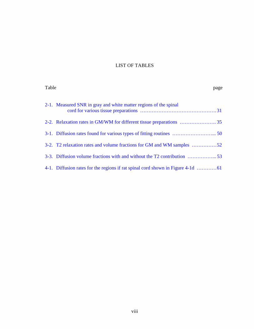
LIST OF TABLES
Table page
2-1. Measured SNR in gray and white matter regions of the spinalcord for various tissue preparations ………………………………………. 31
2-2. Relaxation rates in GM/WM for different tissue preparations …………………. 35
3-1. Diffusion rates found for various types of fitting routines ……………………... 50
3-2. T2 relaxation rates and volume fractions for GM and WM samples ……………52
3-3. Diffusion volume fractions with and without the T2 contribution ……………... 53
4-1. Diffusion rates for the regions if rat spinal cord shown in Figure 4-1d …………61
ix
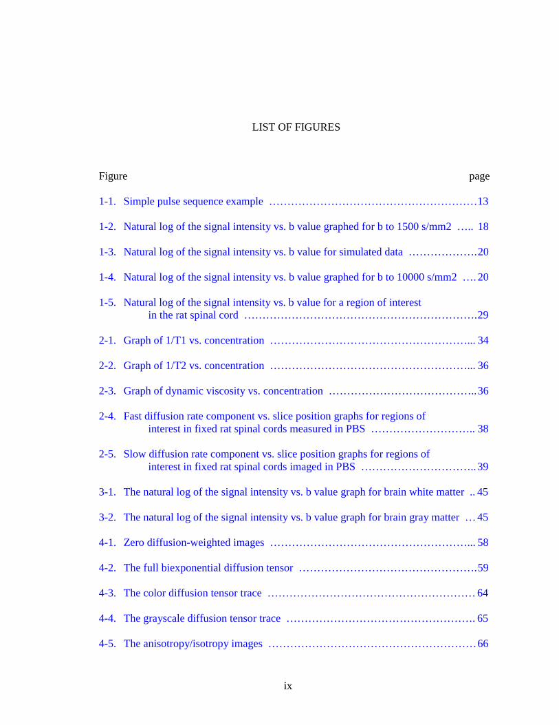
LIST OF FIGURES
Figure page
1-1. Simple pulse sequence example …………………………………………………13
1-2. Natural log of the signal intensity vs. b value graphed for b to 1500 s/mm2 ….. 18
1-3. Natural log of the signal intensity vs. b value for simulated data ……………….20
1-4. Natural log of the signal intensity vs. b value graphed for b to 10000 s/mm2 …. 20
1-5. Natural log of the signal intensity vs. b value for a region of interestin the rat spinal cord ……………………………………………………….29
2-1. Graph of 1/T1 vs. concentration ………………………………………………... 34
2-2. Graph of 1/T2 vs. concentration ………………………………………………... 36
2-3. Graph of dynamic viscosity vs. concentration …………………………………..36
2-4. Fast diffusion rate component vs. slice position graphs for regions ofinterest in fixed rat spinal cords measured in PBS ……………………….. 38
2-5. Slow diffusion rate component vs. slice position graphs for regions ofinterest in fixed rat spinal cords imaged in PBS …………………………..39
3-1. The natural log of the signal intensity vs. b value graph for brain white matter .. 45
3-2. The natural log of the signal intensity vs. b value graph for brain gray matter …45
4-1. Zero diffusion-weighted images ………………………………………………... 58
4-2. The full biexponential diffusion tensor ………………………………………….59
4-3. The color diffusion tensor trace ………………………………………………… 64
4-4. The grayscale diffusion tensor trace ……………………………………………. 65
4-5. The anisotropy/isotropy images …………………………………………………66
x
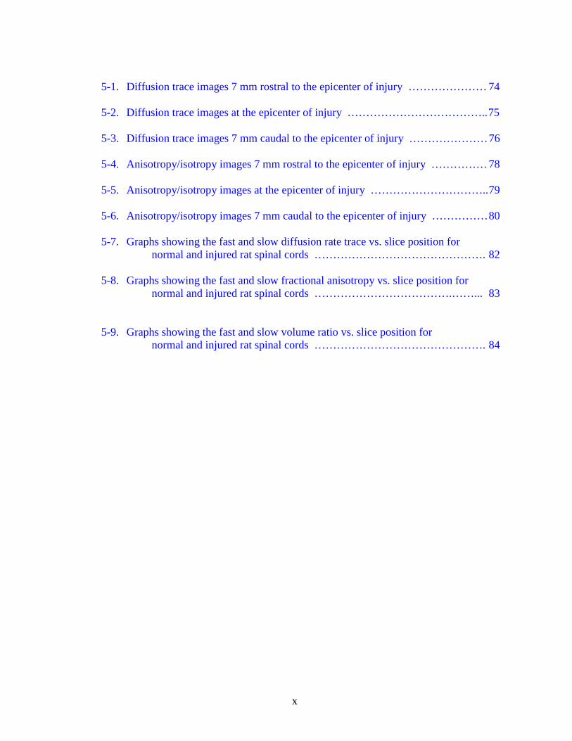
5-1. Diffusion trace images 7 mm rostral to the epicenter of injury ………………… 74
5-2. Diffusion trace images at the epicenter of injury ………………………………..75
5-3. Diffusion trace images 7 mm caudal to the epicenter of injury …………………76
5-4. Anisotropy/isotropy images 7 mm rostral to the epicenter of injury ……………78
5-5. Anisotropy/isotropy images at the epicenter of injury …………………………..79
5-6. Anisotropy/isotropy images 7 mm caudal to the epicenter of injury ……………80
5-7. Graphs showing the fast and slow diffusion rate trace vs. slice position fornormal and injured rat spinal cords ………………………………………. 82
5-8. Graphs showing the fast and slow fractional anisotropy vs. slice position fornormal and injured rat spinal cords ……………………………….……... 83
5-9. Graphs showing the fast and slow volume ratio vs. slice position fornormal and injured rat spinal cords ………………………………………. 84
xi
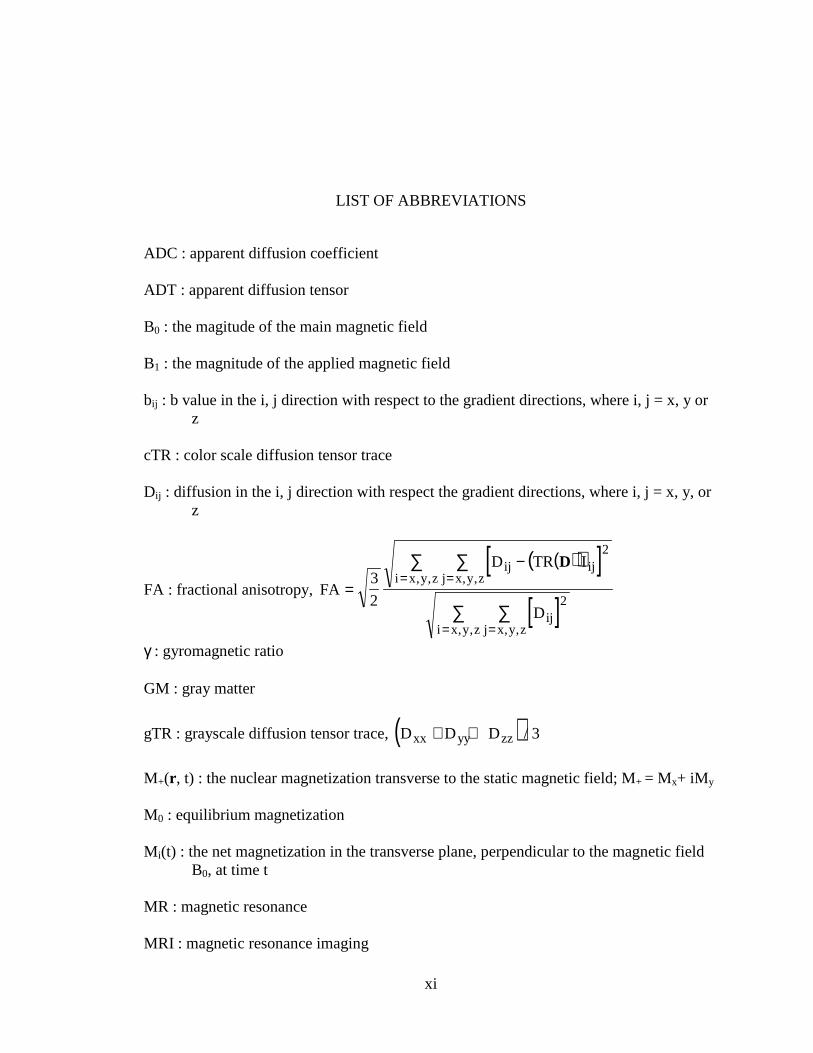
LIST OF ABBREVIATIONS
ADC : apparent diffusion coefficient
ADT : apparent diffusion tensor
B0 : the magitude of the main magnetic field
B1 : the magnitude of the applied magnetic field
bij : b value in the i, j direction with respect to the gradient directions, where i, j = x, y orz
cTR : color scale diffusion tensor trace
Dij : diffusion in the i, j direction with respect the gradient directions, where i, j = x, y, orz
FA : fractional anisotropy,
( )( )[ ][ ]
FA
D TR I
D
ij ijj x y zi x y z
ijj x y zi x y z
=
−==
==
∑∑
∑∑
3
2
2
2
D, ,, ,
, ,, ,
γ : gyromagnetic ratio
GM : gray matter
gTR : grayscale diffusion tensor trace, ( )D D Dxx yy zz+ + / 3
M+(r, t) : the nuclear magnetization transverse to the static magnetic field; M+ = Mx+ iMy
M0 : equilibrium magnetization
Mi(t) : the net magnetization in the transverse plane, perpendicular to the magnetic fieldB0, at time t
MR : magnetic resonance
MRI : magnetic resonance imaging
xii
Mz(t) : magnetization along the longitudinal magnetic field at time
NA : number of averages
NMR : nuclear magnetic resonance
PBS : phosphate buffered saline solution
RF : radio frequency
SNR : signal:to:noise ratio
τc : correlation time; the order of time it takes a molecule to turn through 1 radian, or thetime for a molecule to move through a distance comparable to it’s dimensions
T : tortuosity
TE : echo time
TR : repetition time
VR : volume ratio, ( )
( )[ ]VR
Deter ant
TR=
min
/
D
D 3 3
WM : white matter
ω0 : Larmor frequency; ω0 = γ B0
xiii
Abstract of Dissertation Presented to the Graduate Schoolof the University of Florida in Partial Fulfillment of theRequirements for the Degree of Doctor of Philosophy
MAGNETIC RESONANCE IMAGING AND SPECTROSCOPYFOR THE STUDY OF TRANSLATIONAL DIFFUSION:
APPLICATIONS TO NERVOUS TISSUE
By
Elizabeth L. Bossart
August 1999
Chairman: T.H. MareciMajor Department: Physics
In all stages of trauma and disease in the brain and spinal cord, it is important to
know the amount of the physical damage, how far the damage will extend, and how the
structural changes relate to the final amount of functionality. Though it is fairly
straightforward to measure this damage ex vivo through histological sectioning,
assessment of internal physical damage in vivo has been difficult to do. The innovation
of magnetic resonance (MR) imaging, in particular the measurement of water diffusion,
has been an important step towards quantifying structural changes in living systems.
Water diffusion, once considered a single diffusion rate (or single diffusion rate
tensor) process, appears to be a multiple diffusion rate process. To the limits of the
gradients available (300 mT/m), two unique diffusion regimes have been seen in fixed
CNS tissue: a fast diffusing component and a slow diffusing component. Others have
speculated that the fast and slow diffusing components in tissue represent diffusion in the
extracellular and intracellular spaces, respectively.
xiv
The aim of these studies was to find the best tissue preparation for ex vivo
measurements, determine the best model with which to fit diffusion studies done on CNS
tissue, and to provide a basic understanding of the information contained in the fast and
slow diffusion compartments. These measurements should provide a solid background
for future in vivo experiments, allowing a better understanding of the information
provided by the fast and slow diffusion components. This will be useful for
understanding the role of diffusion in normal tissue and for quantifying changes due to
trauma, which could lead to better diagnostic techniques in the future.
1
CHAPTER 1INTRODUCTION
Observations of soft tissues in vivo were difficult prior to the advent of 1H
magnetic resonance imaging (MRI; Bottomley, 1982; Callaghan, 1991; Hinshaw & Lent,
1983; Lauterbur, 1973). However MRI techniques were needed to quantify the
differences between normal and abnormal tissue. Among the techniques that have been
used to show contrast in biological tissues are the more conventional T1 relaxation and T2
relaxation methods (Akber, 1996; Becerra et al., 1995; Bottomley et al., 1984; Moseley et
al., 1984; Willcott, 1984), and more recent translational water diffusion (Callaghan, 1991;
Le Bihan et al., 1993; Moseley et al., 1990; Stejskal, 1965; Stejskal & Tanner, 1965;
Torrey, 1956). For the measurement of changes due to diffuse injury (i.e. stroke or
edema that causes cell swelling), T1- and T2-weighted images show very few changes
from normal tissue (Becerra et al., 1995; Moseley et al., 1990; Pierpaoli et al., 1996). In
these cases, translational water diffusion imaging better characterizes the changes from
normal tissue (Ford et al., 1994; Kirsch et al., 1991; Moseley et al., 1990; Pattany et al.,
1997; Pierpaoli et al., 1996; van Gelderen et al., 1994).
Translational water diffusion has been used to define solid porous media samples
(Borgin et al., 1996; Ek et al., 1994; Helmer et al., 1995; Latour et al., 1993; Latour et al.
1994; Mitra et al., 1993; Mitra et al., 1992) and to look at biological tissues (Basser et al.,
1994a & 1994b; Basser et al., 1993; Inglis et al., 1997; Kirsch et al., 1991; Moseley et al.,
2
1990; Norris et al., 1994; Pattany et al., 1997; Pierpaoli et al., 1996; Szafer et al., 1995a
and 1995b). Measurements of diffusion coefficients both in vivo and in vitro have aided
in elucidating structure in tissues such as brain and spinal cord (Basser et al., 1993;
Basser et al., 1994b; Chenevert et al., 1990; Ford et al., 1994; Gulani et al., 1997; Inglis
et al., 1997; Kirsch et al., 1991; Le Bihan et al., 1993; Moseley et al., 1990; Ono et al.,
1995; Pattany et al., 1997; Pierpaoli & Basser, 1996; Pierpaoli et al., 1996; Szafer, et al.
1995a & 1995b; Thompson et al., 1987; van Gelderen et al., 1994). By taking a series of
diffusion-weighted images, it is possible to calculate the apparent diffusion coefficient
(ADC) for water molecules moving in the direction of the applied diffusion-weighted
gradients. ADC images have been measured for many tissues (Norris et al., 1994; Szafer
et al., 1995a & 1995b; Pattany et al., 1997). However, if the tissue being looked at is
anisotropic, the ADC values are dependent on the orientation of the structure with respect
to the gradient axes. Because imaging gradients will cause some diffusion cross-terms,
an ADC is only an approximation of a complete apparent diffusion tensor (ADT). A full
ADT map of a tissue gives an indication of the fiber tract orientations within the tissue
(Basser et al., 1993; Basser et al., 1994b; Inglis et al., 1997; Kirsch et al., 1991; Moseley
et al., 1990; Pierpaoli et al., 1996). ADC and ADT mapping have been used extensively
to characterize both brain and spinal cord tissue (Basser et al., 1993; Basser et al., 1994b;
Inglis et al., 1997; Kirsch et al., 1991; LeBihan et al., 1993; Moseley et al., 1990;
Pierpaoli et al., 1996).
Diffusion-weighted imaging and spectroscopy are two of the methods thought to
give an indication of function in both pre- and post- injury spinal cords. ADC and ADT
maps of these tissues both in vivo, in vitro and ex vivo have been studied to this end. In
3
order to compare ex vivo and in vivo measurements of diffusion, more must be
understood about the effects that fixation has on tissue samples. To understand the
fixation effects better, relaxation measurements should be made both on fixative solutions
and on fixed tissue. The measurements on fixative and fixed tissue should aid in the
understanding of how fixation changes the tissue, leading to a better understanding of the
diffusion in fixed tissue. The diffusion maps may be able to give some understanding of
the underlying tissue structure and processes, but first more must be understood about the
diffusion of water through a tissue. In particular, a better understanding is needed of how
relaxation, compartmentalization, exchange and anisotropy effects the diffusion within
tissues.
This introduction begins by outlining different relaxation processes (including
spin-lattice relaxation T1, and spin-spin relaxation T2), and explaining some of the
mechanisms that affect those relaxation processes. Next, the steps necessary to create an
apparent diffusion tensor will be described, followed by a sketch of the inherent problems
in the monoexponential model created by Stejkal and Tanner. The current models that
are used to fit diffusion data are presented and analyzed. From this discussion comes the
presentation of what must be elucidated in order to have a complete model of diffusion in
biological tissue. Finally, a brief outline of the studies done will be presented.
Introduction to Relaxation
Before getting too far into the descriptions of relaxation, one thing should be
noted. In this work a symbol B (e.g. B0) will be called the magnetic field. Although
calling B the magnetic field is not unusual, it is actually a misnomer. In fact, B is the
magnetic flux density, or magnetic inductance, through a material, and is given by the
4
equation B = µ(H + M) where µ is the permeability of the material, M is the
magnetization of the material, and H is the magnetic field strength. Getting back to
relaxation, a resonant radio frequency (RF) pulse effects a spin system by disturbing it
from its thermal equilibrium state. Equilibrium can be restored via several types of
relaxation processes. The following pages will contain a summary of two relaxation
processes, T1 relaxation and T2 relaxation, then describing some of the mechanisms that
cause changes in these relaxation rates (i.e. T2* relaxation, dipole-dipole interactions,
exchange).
Description of T1 Relaxation
T1, “spin-lattice,” or longitudinal relaxation is characterized by the return of the
net magnetization to the ground state (i.e. the state where the net magnetization is along
the main magnetic field) from the high-energy state induced by a RF pulse. For a set of
mutually independent nuclei coupled to a thermal bath, T1 relaxation can be defined as
( )dM
dt
M M
Tz z= −
− 0
1[1-1]
with the solution
( ) ( ) ( )M t M e M ez zt T t T= + −− −0 11 1
0/ / [1-2]
where M0 is the equilibrium magnetization along the longitudinal magnetic field B0
(which is assumed to be along the z-axis), and Mz(t) is the magnetization along the
longitudinal magnetic field at time t. This means that at time t = T1, approximately 63%
of the magnetization has returned to the ground state. The spin system is considered to
be fully relaxed in the longitudinal direction after 3 to 5 T1 periods has passed.
5
T1 relaxation is magnetic field strength dependent and is fastest when the nuclear
motion, or tumbling rate, matches the Larmor frequency (ω0). At this tumbling rate, T1
reaches its characteristic minimum. The Larmor frequency is the precessional frequency
of a nucleus in a magnetic field. It is governed by the equation ω0 = γ B0 where γ is the
gyromagnetic ratio for the nucleus and B0 is the strength of the magnetic field. As the
strength of the magnetic field increases, so does the Larmor frequency. When the Larmor
frequency increases, the characteristic T1 minimum gets longer. Therefore, the higher the
magnetic field, the longer it takes for a nucleus to relax in T1.
Description of T2 Relaxation
For a perfectly homogeneous magnetic field, B0, the decay of magnetization in the
x-y plane is governed by T2, “spin-spin,” or transverse relaxation. T2 relaxation is
characterized by adjacent spins in high and low energy states exchanging energy without
losing that energy to the surrounding lattice. For a set of mutually independent nuclei
coupled to a thermal bath, T2 relaxation can be defined as
dM
dt
M
Ti i= −
2 [1-3]
with solution
( ) ( )M t M ei it T= −0 2/ [1-4]
where i = x or y and Mi(t) is the net magnetization in the transverse plane (along the i-
axis), perpendicular to the magnetic field B0, at time t. This means that after time t = T2,
the net magnetization in the transverse plane has been reduced by approximately 63%.
As with longitudinal relaxation, the spin system is considered to be fully relaxed in the
transverse plane after 3 to 5 T2 periods has passed.
6
In practice, however, the B0 field is inhomogeneous. This means that in different
parts of the sample the nuclei experience disparate magnetic fields, causing the nuclei to
precess at slightly different frequencies. The result is a signal loss due to the dephasing
of individual magnetizations. The consequence of the dephasing is a loss in transverse
magnetization at a rate that is greater than that due to T2 relaxation alone (i.e. the free
induction decay, FID, disappears more rapidly than it would due to T2 relaxation alone).
This loss is known as T2* relaxation and is characterized by the following equation
( )1 1
2 2T TB* = + γ∆ [1-5],
where ∆B is the inhomogeneous variation in the magnetic field. T2* relaxation results in
an inhomogeneous broadening in the MR spectrum, or severe distortions in MR images
when the data is taken at a narrow bandwidth (Callaghan, 1993). Unlike the irreversible,
homogeneous broadening due to T1 and T2 relaxation processes, this type of broadening
is ordered and can be “undone” by the use of an appropriate pulse sequence.
Like T1, T2 is magnetic field dependent. Transverse relaxation time is always less
than or approximately equal to the longitudinal relaxation time. For pure water, the two
relaxation times for 1H NMR are approximately equal, but for biological tissues T2 is
almost always less than T1.
Relaxation Processes
Exchange Processes
Protons in water molecules experience two types of interactions: (1) dipolar
interaction with protons on the same molecule and (2) intermolecular interaction from
protons in neighboring molecules (Kaplan & Fraenkel, 1980; Andrew, 1958; Callaghan,
7
1993). These interactions fluctuate as the water molecule diffuses via rotational and
translational motions. For free water, the rotational correlation time (the time it takes for
the molecule to turn through a radian) is much shorter than the Larmor period (1/ω0
where ω0 = γ B0), so the line width is extremely narrow and T1 §�72. An impurity in the
water, such as oxygen, will act as a relaxation center for the water. The dipolar
interaction between the proton and the impurity ionic moment is modulated by the
relative motion between the water and the ion. This interaction causes a shortening of the
relaxation times T1 and T2.
Water molecules closely associated with larger molecules or solid surfaces (i.e.
bound water) will tumble more slowly. The slower rotational motion leads to a reduction
in T1 and T2 relaxation times. This shortening continues until the correlation time (i.e.
the time it takes a molecule to turn through 1 radian, or the time for a molecule to move
through a distance comparable to it’s dimensions; Andrew, 1958) for the dipolar
fluctuation is approximately equal to the Larmor period (τc §���ω0). When the correlation
time for the dipolar fluctuation equals the Larmor period, T1 relaxation reaches its
characteristic minimum.
Water molecules in close proximity to solid surfaces and slowly moving
macromolecules will have their proton relaxation rates thoroughly affected. Slowing of
reorientational motion in water will inevitably lead to an altered proton relaxation for this
phase. Translational diffusion induces an exchange of molecules between the bound and
free phases. Rotational motion in the bound phase can be quite slow (i.e. correlation
times are much longer than the Larmor period), so divergence of T1 and T2 relaxation
occurs with T1 becoming significantly longer than T2.
8
Dipolar Interactions
The intrinsic magnetic moment associated with each nuclear spin dipole exerts a
large influence on its neighbors via the magnetic field produced by this dipole acting on
the dipole moments of remote spins (Callaghan, 1993; Tycko, 1994; Kaplan & Fraenkel,
1980; Wasylichen, 1987). For solids, where inter-nuclear distances are fixed, this process
dominates the line shape. In all liquids except the most viscous, the tumbling motion of
the molecules is rapid, and the dipolar interaction strength is comparatively weak.
Therefore, the dipolar interactions do not contribute to the broadening of the line shape.
However, for viscous liquids, where tumbling is slower, dipolar interactions begin to take
effect, shortening T2.
Quadrupolar Interactions
A nucleus with spin > 1/2 possesses an electric quadrupole moment (Wasylichen,
1987; Tycko, 1994). The quadrupole moment is collinear with the magnetic dipole
moment for the nucleus. For these nuclei, the interaction between the nuclear quadrupole
moment and fluctuating electric field gradients provide a source for nuclear relaxation.
In fact, for these nuclei, quadrupolar interactions are the principal contributor to spin
relaxation.
Chemical Shielding Anisotropy
Atomic or molecular electron clouds interact with nuclear spin angular
momentum (Callaghan, 1993; Wasylichen, 1987). These interactions characterize the
local electronic environment for an atom or molecule. The principle influence of the
9
surrounding electron cloud is magnetic shielding which results when electronic orbitals
are perturbed by an applied magnetic field. This phenomenon results in chemical
screening or shielding. The local field of a nucleus with less than tetrahedral symmetry
will be dependent on the orientation of the molecule in the applied magnetic field.
Reorientation of the molecule results in a fluctuation of the field at the nucleus, providing
a source for relaxation.
Scalar Relaxation
The finest structural details observed in the liquid state NMR spectroscopy are
from scalar spin-spin coupling or J coupling (Wasylichen, 1987). Indirect interaction
between two nuclei, I and S, is mediated by the electrons present in the molecular orbital.
Nuclear spin causes a slight polarization in the electron cloud. This electron
delocalization is transmitted to neighboring molecular nuclei, leading to the spin-spin
interaction. Fluctuations in the magnetic field at some nucleus I arise due to one of two
interactions. Either the coupling between the nuclei is time dependent due to rapid
chemical exchange (scalar relaxation of the first kind), or one nucleus has a T1 relaxation
time that is short compared to the inverse of the scalar coupling between the nuclei
(scalar relaxation of the second kind). Scalar coupling of the second kind is often a
reason for T2 being much less than T1.
Introduction to Diffusion
Now that relaxation mechanisms have been treated, it is time to treat translational
water diffusion. In diffusion, particles move from one location to another as a result of
random motion due to thermal or equilibrium processes. Using magnetic resonance, this
10
random process can be tracked. In the following discussion, a background of diffusion
will be presented, followed by the methods used to collect and process MR diffusion-
weighted data. Afterwards, the shortcomings of the monoexponential diffusion
formulation are presented, and some competing descriptions are explored.
The Solution to the Bloch-Torrey Equation
The Bloch-Torrey equation gives a generalized treatment of diffusion and flow
through a sample due to magnetic fields (Torrey, 1956; Callaghan, 1991). In the case of
isotropic diffusion and spatially independent velocities, this equation reduces to
( ) ( ) ( ) ( ) ( )t,Mt,MDT
t,Mt,Mi
t
t,M 2
2rvr
rrgr
r++
++
+ ⋅∇−∇+−⋅γ−=∂
∂[1-6]
where D is the diffusion, v is the velocity of spins due to flow, and M+(r, t) is the nuclear
magnetization transverse to the static magnetic field. This is written in complex notation
as M+ = Mx+ iMy. The solution for this equation has the form
( ) ( )[ ]M t S t i t dtt
Tt
+ = − ⋅ ′ ′ −
∫( , ) exp expr r gγ 0
2[1-7].
Putting this solution back into the Bloch-Torrey equation, it is found that
( ) ( )( ) ( )( ) ( )∂∂
γ γS t
tD g t dt i t dt S tt t= − ′ ′ + ⋅ ′ ′
∫ ∫20
2
0v g [1-8].
This differential equation has the solution
( ) ( ) ( )( ) ( )( )S t S D g t dt dt i t dt dttt tt= − ′′ ′′ ′
⋅ ′′ ′′ ′
′ ′∫∫ ∫∫0 20
2
0 00exp expγ γ v g [1-9].
In order to look exclusively at diffusion, consider the case where there is no flow
through the sample, i.e. when v = 0. That is, the following equation needs to be solved
11
( ) ( ) ( )( )S t S D g t dt dttt= − ′′ ′′ ′
′∫∫0 20
2
0exp γ [1-10].
This is generally rewritten as
( ) ( )S t S e bD= −0 [1-11]
where the diffusion-weighting coefficient, b, is defined as
( )( )b g t dt dttt= ′′ ′′ ′′∫∫γ 20
2
0 [1-12].
The Bloch-Torrey equation changes when the diffusion is considered to be
anisotropic. If diffusion is anisotropic, the Bloch-Torrey equation becomes
∂∂
γM
ti M
M
TM M+
++
+ += − ⋅ − + ∇ ⋅ ⋅ ∇ − ∇ ⋅r g D v2
t[1-13]
and the solution to the equation when there is no flow becomes (Callaghan, 1991)
( ) ( )S t S b Dk ijk ijj x y zi x y z
= −
==
∑∑0 exp, ,, ,
[1-14]
where the k subscript indicates the particular gradient strength used to get the signal. The
i and j subscripts on the b and D indicated the direction of the gradients, and the
diffusion-weighting coefficient, bij, is now defined as
( )( ) ( )( ) tdtdtgtdtgb t0 j
t0
t0 i
2ij ′′′′′⋅′′′′γ= ∫∫ ∫
′′[1-15].
Data Collection
In solving the anisotropic form of the Bloch-Torrey equation, a solution was
found that was dependent on b and D, both of which are matrices. If an instantaneous
picture of Dij and Dji (where i ��M��FRXOG�EH�WDNHQ��WKHQ�LW�LV�SRVVLEOH�WKDW�'ij would not
equal Dji. However, an instantaneous picture cannot be taken, and through averaging Dij
12
can be assumed to be equal to Dji. With this assumption, the solution to the Bloch-Torrey
equation becomes
( ) ( ) ( )S t Sb D b D b D
b D b D b Dk
xxk xx yyk yy zzk zz
xyk xy xzk xz yzk yz= −
+ +
+ +
0
2exp
+ [1-16]
There are seven unknowns in this equation: S(0) and the six diffusion coefficients, Dij. In
order to solve this equation the data should be taken with the gradients on in seven
different directions. The directions normally chosen are x, y, z, x = y, x = z, y = z, and x
= y = z (or x = y, x = -y, x = z, x = -z, y = z, y = -z, and x = y = z). The direction of
diffusion can be calculated by looking at diffusion in each of these seven directions.
Theoretically these seven unknowns could be found using only seven data points
(one point in each of the seven directions) and the corresponding seven calculated b
values. This is not the best way however since every minor variation in the data would
cause problems in fitting the data to the equation above. To aid in getting a better fit to
the value of the diffusion rate D, three or more data points are taken in each direction.
Each signal intensity, Sk, is taken at different gradient strengths such that every point has
a different b value. This allows the value of diffusion to be quantified more accurately.
In many of the data sets five different gradient strengths were used in each direction.
This gives a total of thirty-five data points and thirty-five times six b values.
Calculating b Values
After the data has been collected, a fit must be made to find the diffusion
constants in each direction. Before a fit can be made, the b values for each direction must
be found. As was stated previously, the b value is given by Eq. [1-15]. A simple
example will be utilized to illustrate the method used to calculate the b values. For the
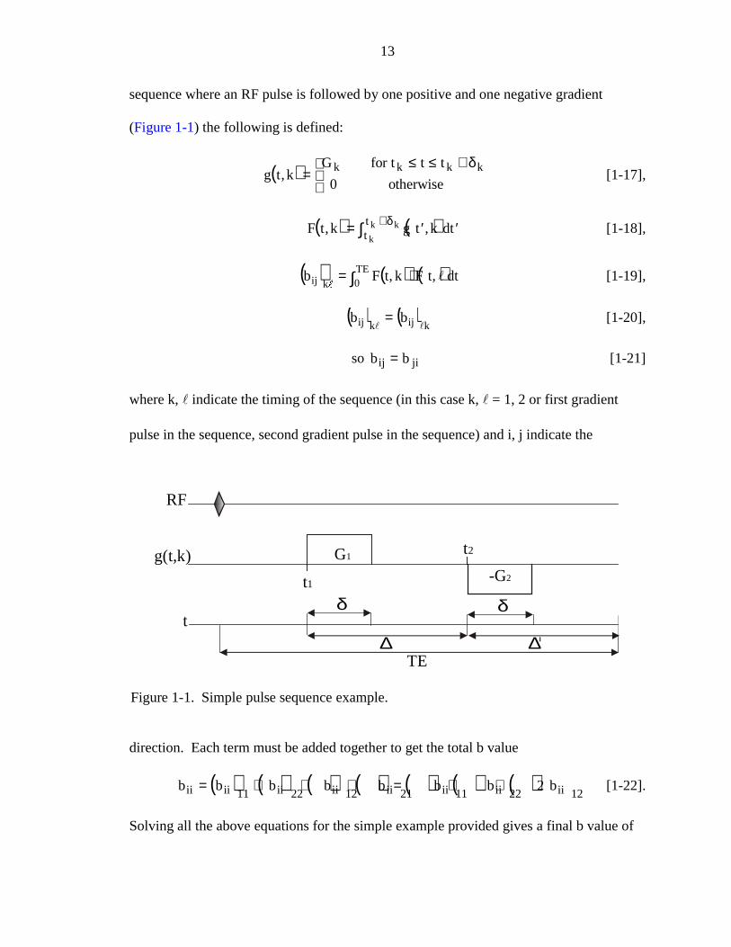
13
sequence where an RF pulse is followed by one positive and one negative gradient
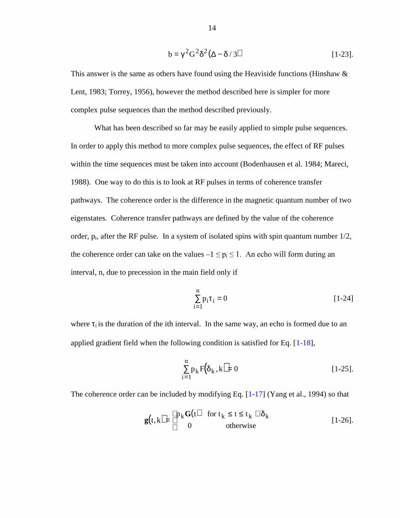
(Figure 1-1) the following is defined:
( )g t kG t tk k k
, =≤ ≤ +
for t
otherwise k δ
0[1-17],
( ) ( )F t k g t k dttt
k
k k, ,= ′ ′+∫ δ[1-18],
( ) ( ) ( )dt,tFk,tFb TE0kij ∫ ⋅= l
l [1-19],
( ) ( )kijkij bbll
= [1-20],
so b bij ji= [1-21]
where k, l indicate the timing of the sequence (in this case k, l = 1, 2 or first gradient
pulse in the sequence, second gradient pulse in the sequence) and i, j indicate the
direction. Each term must be added together to get the total b value
( ) ( ) ( ) ( ) ( ) ( ) ( )b b b b b b b bii ii ii ii ii ii ii ii= + + + = + +11 22 12 21 11 22 12
2 [1-22].
Solving all the above equations for the simple example provided gives a final b value of
Figure 1-1. Simple pulse sequence example.��
RF
g(t,k)
t
t1
t2G1
-G2
δ δ
∆ ∆TE
14
( )b G= −γ δ δ2 2 2 3∆ / [1-23].
This answer is the same as others have found using the Heaviside functions (Hinshaw &
Lent, 1983; Torrey, 1956), however the method described here is simpler for more
complex pulse sequences than the method described previously.
What has been described so far may be easily applied to simple pulse sequences.
In order to apply this method to more complex pulse sequences, the effect of RF pulses
within the time sequences must be taken into account (Bodenhausen et al. 1984; Mareci,
1988). One way to do this is to look at RF pulses in terms of coherence transfer
pathways. The coherence order is the difference in the magnetic quantum number of two
eigenstates. Coherence transfer pathways are defined by the value of the coherence
order, pi, after the RF pulse. In a system of isolated spins with spin quantum number 1/2,
the coherence order can take on the values –1 ��Si ������$Q�HFKR�ZLOO�IRUP�GXULQJ�DQ
interval, n, due to precession in the main field only if
pi ii
nτ
=∑ =
10 [1-24]
where τi is the duration of the ith interval. In the same way, an echo is formed due to an
applied gradient field when the following condition is satisfied for Eq. [1-18],
( )p F kk ki
nδ ,
=∑ =
10 [1-25].
The coherence order can be included by modifying Eq. [1-17] (Yang et al., 1994) so that
( ) ( )g
Gt k
p t t tk k k, =≤ ≤ +
for t
otherwise k δ
0[1-26].
15
With the inclusion of the coherence order, b values can be calculated from any pulse
sequence easily since the specification of the coherence order at each point in the
sequence accounts for the effect of the RF excitation sequence.
Multiple Linear Regression
In order to quantify the rate of diffusion in each of six different directions, the
following set of equations must be solved
( ) ( )
n1,...,=k
yz6
xz5
xy4
zz3
yy2
xx1
i
Dbexp0StS6
1iiikk
======
=
′−= ∑=
[1-27]
once the data has been taken and the b values have been calculated (as before, k indicates
a particular gradient strength) (Stejskal, 1965). Keep in mind that the values bij where i
≠ j are actually multiplied by 2 in order to appear like Eq. [1-16] (e.g. b′4 = bxy + byx =
2bxy). The first thing that must be done to make this problem simpler is to create a linear
equation by taking the natural log of both sides of Equation [1-27]. That means
( ) k
6
1iiik0k Dbyty ε+′−= ∑
=[1-28]
where y(t)k = ln(S(t)k), y0 = ln(S(0)) and εk is the uncorrelated random uncertainty for
measured data points (Montgomery, 1976). The intercept should be redefined as y′0 in
order to take into account the average value of b
∑=
′−=′6
1iii00 Dbyy [1-29]
16
where
∑=
′=′n
1kiki b
n
1b [1-30].
Using this definition for the intercept, the linear equation becomes
( )∑=
ε+′−′−′=6
1ikiiik0k Dbbyy [1-31].
This can be written in matrix form as
by +′= ~[1-32]
where y and ε are vectors of size 1 x n, α is a vector of size 1 x 7, and b′~ is a matrix of
size 7 x n. The matrix b′~ is
( ) ( ) ( )( ) ( ) ( )
( ) ( ) ( )
′−′′−′′−′
′−′′−′′−′′−′′−′′−′
=′
n66n22n11
626222121
616212111
bbbbbb0.1
bbbbbb0.1
bbbbbb0.1
~
L
MOMMM
L
L
b [1-33]
and the vector α is
( ) [ ]Transpose y D D D D D Dα = ′0 1 2 3 4 5 6 [1-34].
A least squares fit is performed to find the values for α. For the least squares fit
( ) ( )byby ′−′−==ε= ∑=
~~L
n
1k
TT2k [1-35].
The derivative of L with respect to α is set equal to zero in order to find the optimum
values of α. This means
bbyb ′′+′−==∂α∂
α
~~2
~20
L TT [1-36].
So
17
ybbb TT ~~~ ′=′′ [1-37].
Solving for α gives the equation in its final form
( ) ybbb T1T ~~~ ′′′=−
[1-38].
The solution to this equation is analytical, and a routine written in IDL
(Interactive Data Language Research Systems Incorporated) will rapidly process the
entire diffusion tensor (64 x 64 matrix, 5 b values in 7 directions) in about half a minute
on an SGI Onyx computer.
Problem with the Mono-Exponential Form
To date, most diffusion weighted images have been taken with b values in the
range of 0 to 1500 s/mm2 (Basser et al., 1994a and 1994b; Basser et al., 1992; Kirsch et
al., 1991; Moseley et al., 1990; Norris et al., 1994; Pattany et al. 1997; Pierpaoli et al.,
1996; Szafer et al., 1995a and 1995b). This is due to the fact that most clinical MR
systems are limited in their gradient strengths. These diffusion measurements seemed to
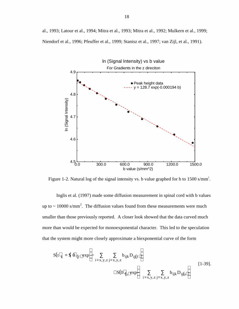
indicate that diffusion is a monoexponential phenomenon, as can be seen in Figure 1-2.
This monoexponential model was described for liquids by Stejskal and Tanner (Stejskal,
1965; Stejskal & Tanner, 1965). The curve in Figure 1-2 was generated from actual data
taken on a sample of human corpus callosum. With the use of better and stronger
gradient systems in both clinical and non-clinical MR systems, diffusion measurements
are being taken with b values up to 40000 s/mm2 (Assaf & Cohen 1998; Bossart et al.,
1999a and 1999b; Borgin et al., 1996; Buckley et al., 1999; Bui et al., 1999; Ek et al.,
1994; Helmer et al., 1995 and 1999; Inglis et al., 1997; Kraemaer et al., 1999; Latour et
18
al., 1993; Latour et al., 1994; Mitra et al., 1993; Mitra et al., 1992; Mulkern et al., 1999;
Niendorf et al., 1996; Pfeuffer et al., 1999; Stanisz et al., 1997; van Zijl, et al., 1991).
Inglis et al. (1997) made some diffusion measurement in spinal cord with b values
up to ~ 10000 s/mm2. The diffusion values found from these measurements were much
smaller than those previously reported. A closer look showed that the data curved much
more than would be expected for monoexponential character. This led to the speculation
that the system might more closely approximate a biexponential curve of the form
( ) ( )( ) ( )
( )( ) ( )
S t S b D
S b D
k f ijk ij fj x y zi x y z
s ijk ij sj x y zi x y z
= −
+ −
==
==
∑∑
∑∑
0
0
exp
exp
, ,, ,
, ,, ,
[1-39].
0.0 300.0 600.0 900.0 1200.0 1500.0b value (s/mm^2)
4.5
4.6
4.7
4.8
4.9
ln (
Sig
nal I
nten
sity
)ln (Signal Intensity) vs b value
For Gradients in the z direciton
Peak height datay = 128.7 exp(-0.000194 b)
Figure 1-2. Natural log of the signal intensity vs. b value graphed for b to 1500 s/mm .2
19
In this equation the f and s subscripts stand for fast and slow diffusion rates, respectively.
In order to get an idea about what happens when a mono-exponential curve fit is
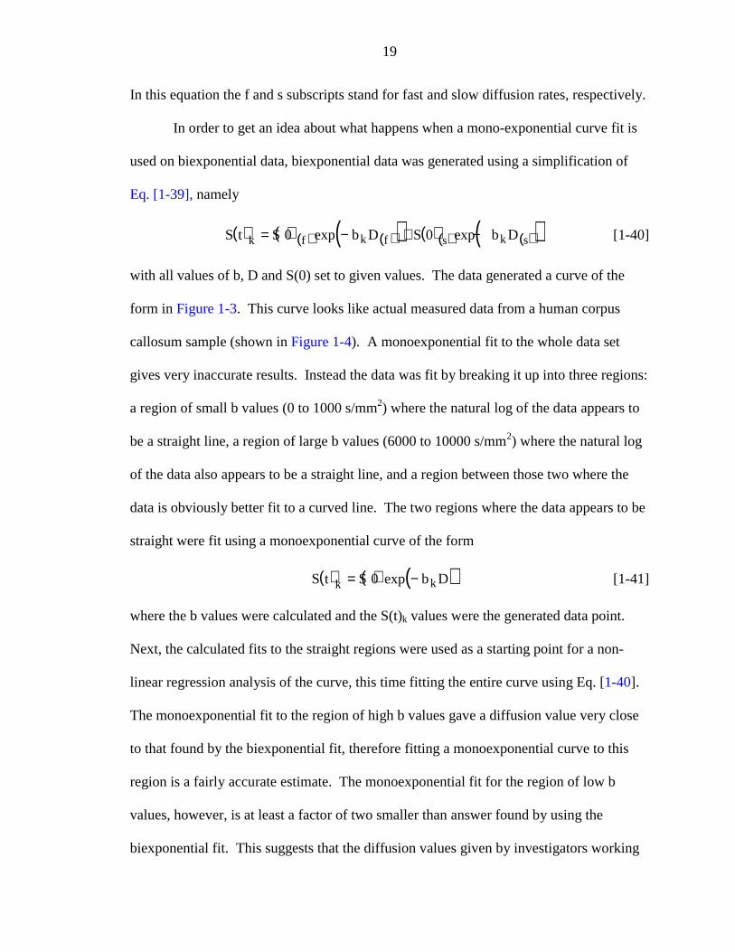
used on biexponential data, biexponential data was generated using a simplification of
Eq. [1-39], namely
( ) ( )( ) ( )( ) ( )( ) ( )( )S t S b D S b Dk f k f s k s= − + −0 0exp exp [1-40]
with all values of b, D and S(0) set to given values. The data generated a curve of the
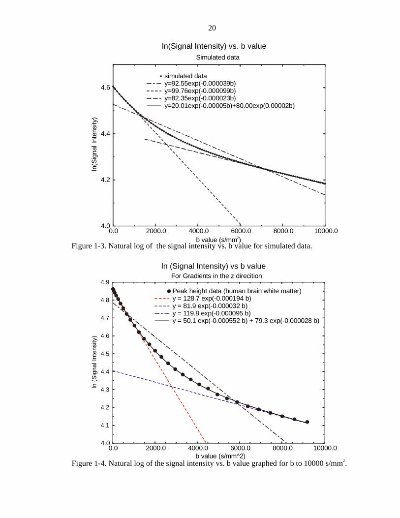
form in Figure 1-3. This curve looks like actual measured data from a human corpus
callosum sample (shown in Figure 1-4). A monoexponential fit to the whole data set
gives very inaccurate results. Instead the data was fit by breaking it up into three regions:
a region of small b values (0 to 1000 s/mm2) where the natural log of the data appears to
be a straight line, a region of large b values (6000 to 10000 s/mm2) where the natural log
of the data also appears to be a straight line, and a region between those two where the
data is obviously better fit to a curved line. The two regions where the data appears to be
straight were fit using a monoexponential curve of the form
( ) ( ) ( )S t S b Dk k= −0 exp [1-41]
where the b values were calculated and the S(t)k values were the generated data point.
Next, the calculated fits to the straight regions were used as a starting point for a non-
linear regression analysis of the curve, this time fitting the entire curve using Eq. [1-40].
The monoexponential fit to the region of high b values gave a diffusion value very close
to that found by the biexponential fit, therefore fitting a monoexponential curve to this
region is a fairly accurate estimate. The monoexponential fit for the region of low b
values, however, is at least a factor of two smaller than answer found by using the
biexponential fit. This suggests that the diffusion values given by investigators working
20
b value (s/mm )2
0.0 2000.0 4000.0 6000.0 8000.0 10000.04.0
4.2
4.4
4.6ln
(Sig
nal I
nten
sity
)
ln(Signal Intensity) vs. b valueSimulated data
simulated datay=92.55exp(-0.000039b)y=99.76exp(-0.000099b)y=82.35exp(-0.000023b)y=20.01exp(-0.00005b)+80.00exp(0.00002b)
Figure 1-3. Natural log of the signal intensity vs. b value for simulated data.
0.0 2000.0 4000.0 6000.0 8000.0 10000.0b value (s/mm^2)
4.0
4.1
4.2
4.3
4.4
4.5
4.6
4.7
4.8
4.9
ln (
Sig
nal I
nten
sity
)
ln (Signal Intensity) vs b valueFor Gradients in the z direcition
Peak height data (human brain white matter)y = 128.7 exp(-0.000194 b)y = 81.9 exp(-0.000032 b)y = 119.8 exp(-0.000095 b)y = 50.1 exp(-0.000552 b) + 79.3 exp(-0.000028 b)
Figure 1-4. Natural log of the signal intensity vs. b value graphed for b to 10000 s/mm .2
21
in the b value range of 0 to 1000 s/mm2 may not be accurate if the actual diffusion rate is
a biexponetial. The diffusion values should be higher than one would anticipate from
looking at such a limited range of data.
Exploring the biexponential behavior of the data is the next task. In the following
three sections, different models will be discussed that propose to fit the curvilinear data.
Each model has its positive and negative aspects, but each is incomplete. These aspects
of the models will be described and explored briefly.
Multiexponential Diffusion
Porous Media Theory
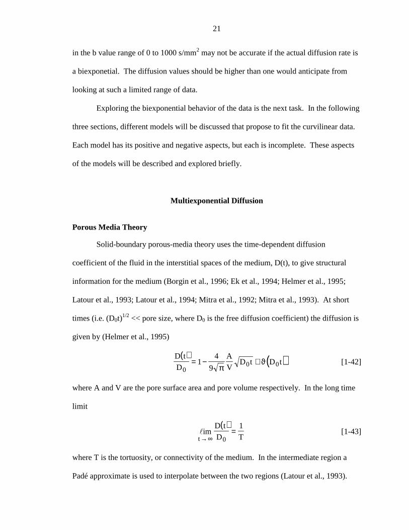
Solid-boundary porous-media theory uses the time-dependent diffusion
coefficient of the fluid in the interstitial spaces of the medium, D(t), to give structural
information for the medium (Borgin et al., 1996; Ek et al., 1994; Helmer et al., 1995;
Latour et al., 1993; Latour et al., 1994; Mitra et al., 1992; Mitra et al., 1993). At short
times (i.e. (D0t)1/2 << pore size, where D0 is the free diffusion coefficient) the diffusion is
given by (Helmer et al., 1995)
( ) ( )D t
D
A
VD t D t
00 01
4
9= − +
πϑ [1-42]
where A and V are the pore surface area and pore volume respectively. In the long time
limit
( )lim
D t
D Tt→∞=
0
1[1-43]
where T is the tortuosity, or connectivity of the medium. In the intermediate region a
Padé approximate is used to interpolate between the two regions (Latour et al., 1993).
22
This model has been demonstrated to work very well for solid systems that have
liquids or gases filling their interstitial spaces. Many of the experiments performed to fit
this model varied diffusion time instead of gradient strength. Usually the experiments
run on tissue vary gradient strength and leave the time constant. This makes the
experiments a bit difficult to compare with the tissue measurements. Latour et al. (1993)
used this model to fit data from water in the “pores” of a monosized sphere pack (spheres
a diameter of 96 µm), and water in packed human red blood cells (1994). Helmer et al.
(1995) extol the virtues of this model in its suggestion that the curvilinear appearance of
the diffusion rate vs. b value data is due to geometrical structure within the sample rather
than the number of distinct compartments within the sample. However, they do not
attempt to fit their biological tissue data (sampling from non-necrotic and necrotic
regions of a tumor) to this model. That suggests some difficulty in applying this model to
tissues. Tissues are not just porous, but have semipermeable membranes that allow the
passage of some substances through but not others. This implies that the cell membrane
is impermeable to all solutes except for very small, uncharged molecules. So diffusional
motion through biological tissue is not as simple as in porous media.
Inside the cell, the diffusion rate is slowed due to water molecules running into
proteins, organelles and other substances contained within the cell. The diffusion rate
outside of the cell will be slowed by the closeness of the cells to one another, similar to
the manner in which the diffusion rate was changed by moving around the packed beads.
Both rates should be modified by exchange between the cells and the surrounding
extracellular space, and the exchange rate will be effected by the permeability of the
membrane in question. The porous media theory does not take into account the
23
cytoskeletal structures or other substances within the cells, nor does it include exchange.
As well as this theory works for solid substances, it is not clear that it will work for
biological systems because of these aforementioned facts.
An Analytical Model of Restricted Diffusion
The second model was created by Stanisz et al. (1997 and 1998) to look at
restricted diffusion in bovine optic nerve using a three pool model. The model has two
intracellular compartments (spherical and ellipsoidal cells) and one extracellular
compartment. One of the assumptions made in this model is that the diffusion rates for
the two intracellular compartments are equal in magnitude, and the intracellular diffusion
rate is different than the extracellular diffusion rate. This model has three analytical
parts: (a) water motion in the extracellular spaces; (b) restricted diffusion inside cells;
and (c) exchange between the intracellular and extracellular compartments.
The diffusion rate in the extracellular compartment is found by
DD
TEAPP E= [1-44]
which is the same equation as was given for the long-time behavior in porous-media
theory (Helmer et al., 1995). The tortuosity is orientation dependent. This accounts for
anisotropy in the observed data.
The intracellular diffusion rate is modeled using a one-dimensional
approximation. The model is for restricted diffusion within an infinite parallel
membrane. The equation for the diffusion rate is (Stanisz et al., 1997)
24
( )( )
( ) ( ) ( )( ) ( )( )
Db
n
G
G
G n DG
G n
JAPP
J
J
J IJ
nJ
Jn
= −
−
−
− −
−
∑
1
21
41 1
2
2 2 22 2 2
2
l
l
l
ll
l
l
cos
expcos
γ δ
γ δ
γ δ πγ δ
γ δ π +
∆[1-45]
where l is the average restricted distance the diffusing species experiences within a cell
of type J = S (spheres), T (ellipsoids).
The exchange rate, K, between the intracellular compartment and the extracellular
compartment is found by multiplying the membrane permeability, P, by the surface-to-
volume ratio A/V. This exchange rate is used by the modified Bloch equations which
were extended according to Karger et al. (1988) to be
dM
dtG D M K M K MT
TAPP
T T T E E= − − +γ δ2 2 2 [1-46]
dM
dtG D M K M K MS
SAPP
S S S E E= − − +γ δ2 2 2 [1-47]
dM
dtG D M K M K M K ME
EAPP
E E E S S T T= − − + +γ δ2 2 2 [1-48]
with the appropriate initial conditions. Here, E represents the extracellular compartment,
S represents the spherical intracellular compartment and T represents the ellipsoidal
intracellular compartment. Using a Monte Carlo simulation, nine parameters are fit into
the three parts of this model. These nine parameters are the intracellular diffusion rate
(DI), the long and short axes of the ellipsoidal cells (aT(⊥) and aT(||)), the diameter of the
spherical cells (aS), the volumes of each cell type (VT and VS), the membrane
permeability of each cell type (PT and PS), and the extracellular diffusion rate (DE).
25
There are a few problems with this model. Stanisz et al. (1997) fit the parameters
to within only 15% using this model. The model seems to fit well at smaller b values, but
the larger the b value, the worse the fit seems to get. That means that the model does not
fit the data quite well enough. Their errors probably stem from two major sources: (a)
the long-time diffusion model used for the extracellular space and (b) the one-
dimensional model used to characterize the diffusion in the intracellular space. The long-
time diffusion model is the same as is used in porous media theory, and the drawbacks of
that model were explained in the previous section. As before, exchange between the
intracellular and extracellular spaces will change how well this model fits the data. The
one-dimensional model used to define diffuison in the intracellular space is inaccurate
because of the infinite parallel barrier approximation that was used. This may be a
reasonable approximation for water travelling down the long axis of an ellipsoid, but it
will not fit as well for water travelling in the small spherical cells, or along one of the
minor axes of the ellipsoid. Also, this model takes into account only very regular shaping
of the cells. Cells are very irregularly shaped, and filed with structures and substances
with which water interacts. True biological systems do not have such regular shapes.
Multiexponential Model
The final model was introduced by Karger et al. (1988) and was reiterated by
Niendorf et al. (1996). Of late, this model has gained popularity, and has been used in
presentations at a few meetings (Bossart et al., 1999a and 1999b; Bui et al., 1999; Helmer
et al., 1999; Kraemer et al., 1999; Mulkern et al., 1999; Pfeuffer et al., 1999). When the
system under consideration is composed of different subregions, then the observed signal
26
attenuation can be given by a superposition of the contributions from individual
subregions
( )S b f bDi ii
( ) exp= −∑ [1-49].
For tissues it can be assumed that the two compartments are an intracellular
compartment and an extracellular compartment. Exchange between the two
compartments occurs on a time scale related to the mean lifetime (τin(ex)) of water
molecules in a compartment. In the short diffusion time limit (t << τin(ex)) the signal is
just a linear superposition of two monoexponentials (Neindorf et al., 1996)
( ) ( ) ( )S b
Sf bD f bDin in ex ex
0= − + −exp exp [1-50].
At the long diffusion time limit (t >> τin(ex)), complete exchange occurs between
the two compartments and the signal attenuation will show a monoexponential
dependence
( ) ( )( )S b
Sb f D f Din in ex ex
0= − +exp [1-51].
In the intermediate range, the signal attenuation appears as the sum of two
monoexponentials as in the short time limit
( ) ( ) ( )S b
Sf bD f bDin in ex ex
0= ′ − ′ + ′ − ′exp exp [1-52];
however, the volume fractions (f′in(ex)) and the diffusion rates (D′in(ex)) in the intermediate
time periods become mixtures of the rates found in the short time limit due to the
exchange of water between the two compartments (Karger et al., 1988). The only thing
lacking in this model is an accounting of the anisotropy. Tensor data taken by our group
27
and by other groups shows that there is anisotropy in some biological samples, otherwise
there would be no difference between the diffusion images along the diagonal of the
tensor. That is to say, the x, y and z images would be exactly the same and the off-
diagonal elements would be zero if the tissue were isotropic. Perhaps the anisotropy
comes from the geometry of the sample, or perhaps it comes from the variety of
substances impeding the diffusion through the tissue sample.
Study Directions
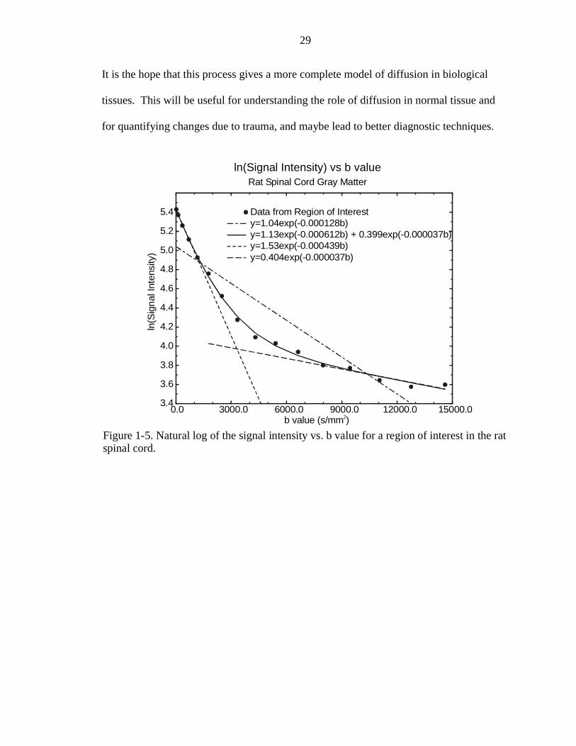
The purpose of this study is to verify that the biexponential model proposed by
Karger et al. (1988) is an accurate one, to adjust the model to take into account anisotropy
in tissues, and to find the roles that compartmentalization, exchange and relaxation play
in diffusion behavior. Although the model proposed by Stanisz et al. (1997 and 1998)
retains some of the characteristics of the Karger model (e.g. assuming distinctly different
diffusion rates in the extracellular and intracellular spaces), it does not seem to fit the data
as closely as the model proposed by Karger et al. (1988). The biexponential model is a
very good two-compartment model with exchange. This model fits well to mono-
directional data taken in rat spinal cord and human corpus callosum (Figures 1-4 and 1-
5). However, as stated before, the model does not adequately explain anisotropic
diffusion in tissues. Also, given large enough diffusion gradients, three or more diffusion
coefficients have been seen. Assaf and Cohen (1998) describe observing a system that
seems to fit the sum of three exponential terms when the gradients are large enough. The
question to answer is whether those different diffusion rates are due to different
compartments or if it is due to other factors. Therefore, the following series of studies are
proposed to aid in determining if this really is a good multicompartment model, to
28
determine how exchange effects the apparent diffusion rate, and to determine how the
anisotropy fits into the model.
1. T1 and T2 relaxation studies of fixative solutions and the effect fixative solutions have
on relaxation in biological tissues were done. These studies will aid in determining
how tissue preparation affects the ex vivo tissue results. It will also help to determine
the best tissue preparation method for comparison with in vivo studies, as well as for
doing histological comparisons.
2. T2 relaxation and diffusion spectroscopy studies were done on human white and gray
matter brain samples. Human brain samples were chosen because nearly
homogeneous tissue samples can be cored from the human brain. The data taken from
brain white and gray matter samples could compare qualitatively with the white and
gray matter in the spinal cord. Pulsed gradient spin-echo spectroscopy was done
because complete data can be taken much more rapidly than with imaging. Also, T2
relaxation imaging experiments are inherently diffusion weighted due to the imaging
gradients used, making the deconvolution of diffusion and relaxation much more
difficult than with spectroscopy studies.
3. Diffusion imaging studies in normal rat spinal cord were done. These studies could
confirm or deny some of the ideas presented in the previous studies on the brain
samples, as well as give the first images of the two different diffusion compartments.
4. Comparison studies of diffusion in normal and injured rat spinal cord were done.
These studies further explore the meaning of the two diffusion compartments, as well
as give some further confirmation of ideas presented in the previous studies.
29
It is the hope that this process gives a more complete model of diffusion in biological
tissues. This will be useful for understanding the role of diffusion in normal tissue and
for quantifying changes due to trauma, and maybe lead to better diagnostic techniques.
0.0 3000.0 6000.0 9000.0 12000.0 15000.0b value (s/mm )2
3.4
3.6
3.8
4.0
4.2
4.4
4.6
4.8
5.0
5.2
5.4
ln(S
igna
l Int
ensi
ty)
ln(Signal Intensity) vs b valueRat Spinal Cord Gray Matter
Data from Region of Interesty=1.04exp(-0.000128b)y=1.13exp(-0.000612b) + 0.399exp(-0.000037b)y=1.53exp(-0.000439b)y=0.404exp(-0.000037b)
Figure 1-5. Natural log of the signal intensity vs. b value for a region of interest in the ratspinal cord.
30
CHAPTER 2FIXATION EFFECTS
Relaxation measurements have been made on both fixed and “fresh” (or unfixed)
tissues ex vivo in order to determine the effects that death and fixation have on tissue as
observed using 1H NMR (Akber, 1996; Baba et al., 1994; Bottomley, et al. 1984; Carvlin
et al., 1989; Fischer et al., 1989; Gyorffy-Wagner et al., 1986; Kamman et al., 1985;
Moseley et al., 1984; Nagara et al., 1987; Pattany et al., 1997; Thickman et al., 1983;
Tovi & Ericsson, 1992; Willcott, 1984). Such measurements provide a greater
understanding of how in vitro and ex vivo tissue studies relate to in vivo tissue studies.
These relaxation experiments on tissue samples in vitro and ex vivo have shown that
tissue death and fixation have a very large effect on the T2 relaxation times and a less
pronounced effect on the T1 relaxation time. However, these early studies did not explore
the reasons for these relaxation changes or the signal-to-noise ratio (SNR) differences
observed between fixed and unfixed tissue samples.
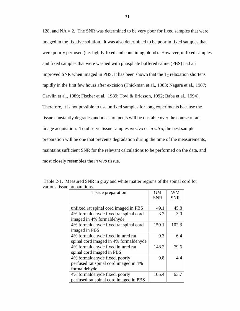
In this study, experiments were performed to find the best tissue preparation for
imaging in vitro. The SNR measurements presented in Table 2-1 show that tissue
preparation has a huge effect on the SNR. Each measurement was performed on a single
sample of this type. The SNR for each tissue preparation was calculated from images
taken at 600 MHz with the following parameters: TR = 3 s, TE = 36 ms, matrix = 128 x
31
128, and NA = 2. The SNR was determined to be very poor for fixed samples that were
imaged in the fixative solution. It was also determined to be poor in fixed samples that
were poorly perfused (i.e. lightly fixed and containing blood). However, unfixed samples
and fixed samples that were washed with phosphate buffered saline (PBS) had an
improved SNR when imaged in PBS. It has been shown that the T2 relaxation shortens
rapidly in the first few hours after excision (Thickman et al., 1983; Nagara et al., 1987;
Carvlin et al., 1989; Fischer et al., 1989; Tovi & Ericsson, 1992; Baba et al., 1994).
Therefore, it is not possible to use unfixed samples for long experiments because the
tissue constantly degrades and measurements will be unstable over the course of an
image acquisition. To observe tissue samples ex vivo or in vitro, the best sample
preparation will be one that prevents degradation during the time of the measurements,
maintains sufficient SNR for the relevant calculations to be performed on the data, and
most closely resembles the in vivo tissue.
Table 2-1. Measured SNR in gray and white matter regions of the spinal cord forvarious tissue preparations.
Tissue preparation GMSNR
WMSNR
unfixed rat spinal cord imaged in PBS 49.1 45.84% formaldehyde fixed rat spinal cordimaged in 4% formaldehyde
3.7 3.0
4% formaldehyde fixed rat spinal cordimaged in PBS
150.1 102.3
4% formaldehyde fixed injured ratspinal cord imaged in 4% formaldehyde
9.3 6.4
4% formaldehyde fixed injured ratspinal cord imaged in PBS
148.2 79.6
4% formaldehyde fixed, poorlyperfused rat spinal cord imaged in 4%formaldehyde
9.8 4.4
4% formaldehyde fixed, poorlyperfused rat spinal cord imaged in PBS
105.4 63.7
32
For multiexponential T2 and multicompartment diffusion experiments, it is
important to have a high SNR (> 60). If the SNR is too low, fitting the data to non-linear
curves is difficult and inconclusive. It is important to understand why these SNR
changes occur in order to avoid these difficulties. The relaxation rates of varying
concentrations of fixative solutions were measured in order to interpret the differences
seen between imaging tissue in fixative solution and PBS. Afterwards, the relaxation rate
for a spinal cord tissue sample fixed with 4% paraformaldehyde solution was measured
both in fixative and in PBS.
Materials and Methods
Relaxation Measurements in Solution
Relaxation times were measured for solutions of formaldehyde (CH2O) and
gluteraldehyde (OCH(CH2)3CHO) at concentrations of 1, 2, 4 and 8 percent. They were
also performed on full, half and quarter Karnowsky’s solution (full Karnowsky’s solution
= 5% gluteraldehyde + 4% formaldehyde). All measurements were performed using a
600 MHz Varian spectrometer with the samples at physiological pH (7.2) and at a
temperature of 25o C. T1 measurements were made using an inversion recovery
sequence, and T2 measurements were made using the Carr-Purcell-Meibloom-Gill
(CPMG) sequence (see Appendix B for the pulse sequences). Each sample spectrum was
performed only once with eight averages.
33
Imaging Measurements in Tissue
The water relaxation measurements in tissue were acquired using an imaging
spin-echo sequence. Repetition time (TR) was arrayed for the T1 measurements, and
echo time (TE) was arrayed for the T2 measurements. These water relaxation
measurements were performed on a single tissue sample with four averages. To provide
the tissue sample, a rat was transcardially exsanguinated with saline solution and heparin,
then perfused with a 4% formaldehyde solution. Water relaxation measurements were
performed on the water within the fixed cord in immersed in fixative solution. The tissue
was then washed with PBS 4 times over a 36 hour period, placed in fresh PBS, and the
water relaxation measurements were repeated.
Finally, rat spinal cord tissue was prepared by exsanguinating in vivo with saline
solution, followed by perfusion with one of three different fixative solutions prior to
removal from the animal: 4% formaldehyde (n = 3), half Karnowsky’s (n = 3) and full
Karnowsky’s solution (n = 3). A total of 9 diffusion experiments were performed. Each
tissue sample was taken from the same spinal cord location, at T13. Following fixation,
these cords were washed with PBS three times over a 36 hour period, and placed in fresh
PBS. A full biexponential diffusion experiment, as described in the Materials and
Methods section of Chapter 4 and Chapter 5, was then performed on these cords at 600
MHz. Numerical data was calculated at specific regions of interest in the cord to find out
if the fixative preparation changes the observed diffusion rates. After the experiments, all
tissue samples were replaced in the fixative solution.
34
Results
Fixative Solution Measurements
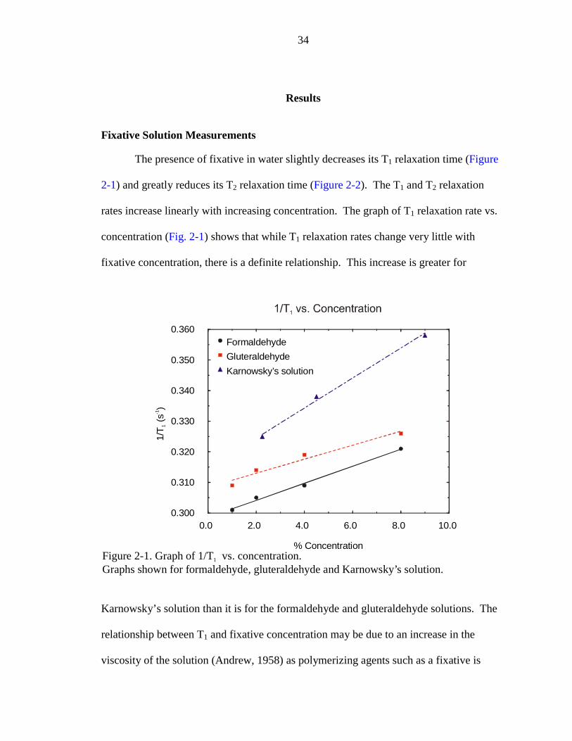
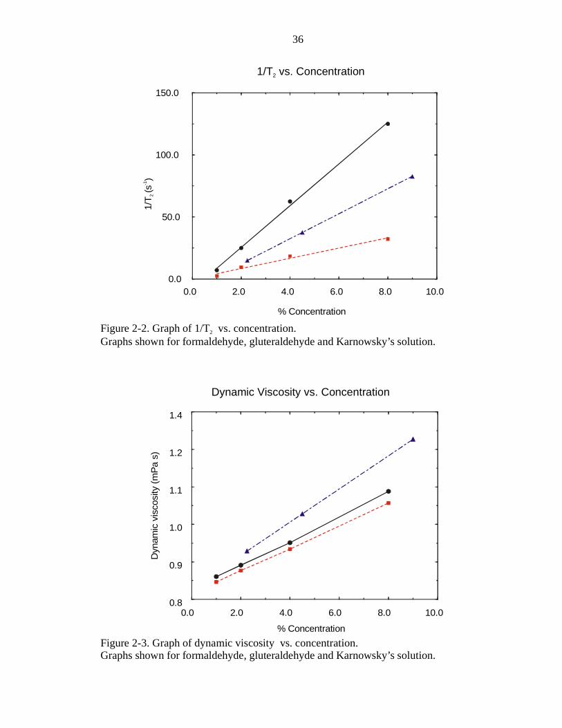
The presence of fixative in water slightly decreases its T1 relaxation time (Figure
2-1) and greatly reduces its T2 relaxation time (Figure 2-2). The T1 and T2 relaxation
rates increase linearly with increasing concentration. The graph of T1 relaxation rate vs.
concentration (Fig. 2-1) shows that while T1 relaxation rates change very little with
fixative concentration, there is a definite relationship. This increase is greater for
Karnowsky’s solution than it is for the formaldehyde and gluteraldehyde solutions. The
relationship between T1 and fixative concentration may be due to an increase in the
viscosity of the solution (Andrew, 1958) as polymerizing agents such as a fixative is
0.0 2.0 4.0 6.0 8.0 10.0
% Concentration
0.300
0.310
0.320
0.330
0.340
0.350
0.360
1/T
(s
)1
-1
Formaldehyde
Gluteraldehyde
Karnowsky’s solution
Figure 2-1. Graph of 1/T vs. concentration.Graphs shown for formaldehyde, gluteraldehyde and Karnowsky’s solution.
1
35
added. To test this hypothesis, the viscosity of each fixative solution was measured at
25o C using a capillary viscometer. The results of the viscosity measurements are shown
on the graph of viscosity vs. fixative concentration in Figure 2-3. The trends seen in the
slopes of the lines on Figure 2-3 are the same as the trends seen in the lines on Figure 2-1
(i.e. Karnowsky’s solution vs. concentration has the steepest slope and formaldehyde
solution vs. concentration has the shallowest slope). The large effect that fixative has on
the T2 relaxation rate of water is most likely due to chemical exchange processes going
on in the solution.
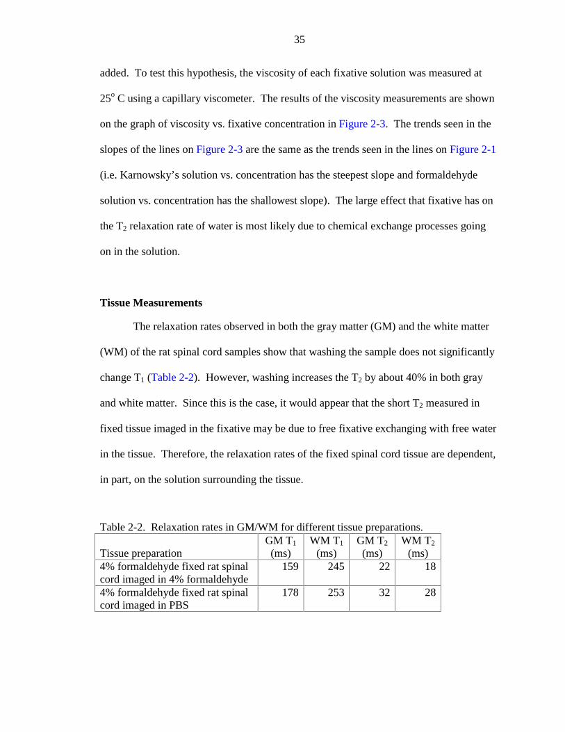
Tissue Measurements
The relaxation rates observed in both the gray matter (GM) and the white matter
(WM) of the rat spinal cord samples show that washing the sample does not significantly
change T1 (Table 2-2). However, washing increases the T2 by about 40% in both gray
and white matter. Since this is the case, it would appear that the short T2 measured in
fixed tissue imaged in the fixative may be due to free fixative exchanging with free water
in the tissue. Therefore, the relaxation rates of the fixed spinal cord tissue are dependent,
in part, on the solution surrounding the tissue.
Table 2-2. Relaxation rates in GM/WM for different tissue preparations.
Tissue preparationGM T1
(ms)WM T1
(ms)GM T2
(ms)WM T2
(ms)4% formaldehyde fixed rat spinalcord imaged in 4% formaldehyde
159 245 22 18
4% formaldehyde fixed rat spinalcord imaged in PBS
178 253 32 28
36
0.0 2.0 4.0 6.0 8.0 10.0
% Concentration
0.0
50.0
100.0
150.0
1/T
(s)
2 -1
1/T vs. Concentration2
Figure 2-2. Graph of 1/T vs. concentration.Graphs shown for formaldehyde, gluteraldehyde and Karnowsky’s solution.
2
0.0 2.0 4.0 6.0 8.0 10.0
% Concentration
0.8
0.9
1.0
1.1
1.2
1.4
Dyn
amic
vis
cosi
ty (
mP
a s)
Dynamic Viscosity vs. Concentration
Figure 2-3. Graph of dynamic viscosity vs. concentration.Graphs shown for formaldehyde, gluteraldehyde and Karnowsky’s solution.
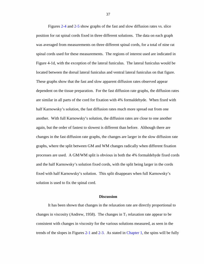
37
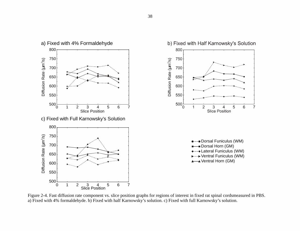
Figures 2-4 and 2-5 show graphs of the fast and slow diffusion rates vs. slice
position for rat spinal cords fixed in three different solutions. The data on each graph
was averaged from measurements on three different spinal cords, for a total of nine rat
spinal cords used for these measurements. The regions of interest used are indicated in
Figure 4-1d, with the exception of the lateral funiculus. The lateral funiculus would be
located between the dorsal lateral funiculus and ventral lateral funiculus on that figure.
These graphs show that the fast and slow apparent diffusion rates observed appear
dependent on the tissue preparation. For the fast diffusion rate graphs, the diffusion rates
are similar in all parts of the cord for fixation with 4% formaldehyde. When fixed with
half Karnowsky’s solution, the fast diffusion rates much more spread out from one
another. With full Karnowsky’s solution, the diffusion rates are close to one another
again, but the order of fastest to slowest is different than before. Although there are
changes in the fast diffusion rate graphs, the changes are larger in the slow diffusion rate
graphs, where the split between GM and WM changes radically when different fixation
processes are used. A GM/WM split is obvious in both the 4% formaldehyde fixed cords
and the half Karnowsky’s solution fixed cords, with the split being larger in the cords
fixed with half Karnowsky’s solution. This split disappears when full Karnowsky’s
solution is used to fix the spinal cord.
Discussion
It has been shown that changes in the relaxation rate are directly proportional to
changes in viscosity (Andrew, 1958). The changes in T1 relaxation rate appear to be
consistent with changes in viscosity for the various solutions measured, as seen in the
trends of the slopes in Figures 2-1 and 2-3. As stated in Chapter 1, the spins will be fully
38
0 1 2 3 4 5 6 7Slice Position
500
550
600
650
700
750
800
Diff
usio
n R
ate
(m
/s)
µ2
a) Fixed with 4% Formaldehyde
Diff
usio
n R
ate
(m
/s)
µ2
Diff
usio
n R
ate
(m
/s)
µ2
0 1 2 3 4 5 6 7Slice Position
500
550
600
650
700
750
800
c) Fixed with Full Karnowsky’s Solution
Dorsal Funiculus (WM)Dorsal Horn (GM)Lateral Funiculus (WM)Ventral Funiculus (WM)Ventral Horn (GM)
Figure 2-4. Fast diffusion rate component vs. slice position graphs for regions of interest in fixed rat spinal cordsmeasured in PBS.a) Fixed with 4% formaldehyde. b) Fixed with half Karnowsky’s solution. c) Fixed with full Karnowsky’s solution.
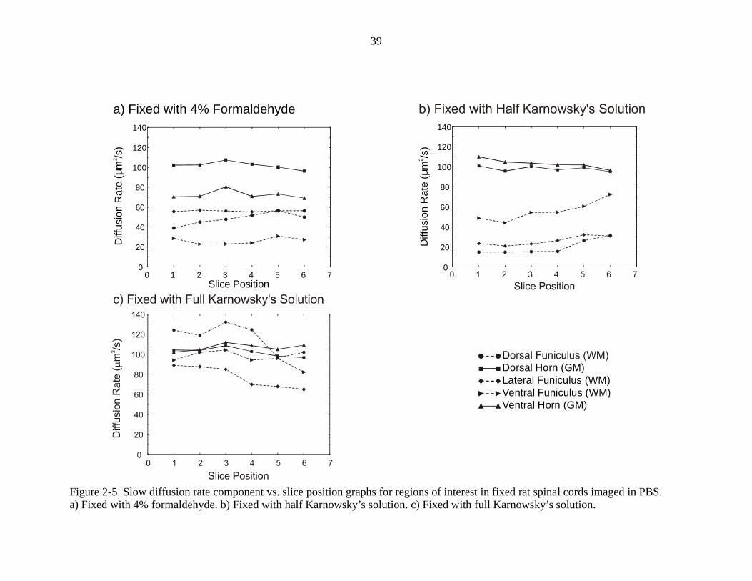
39
Figure 2-5. Slow diffusion rate component vs. slice position graphs for regions of interest in fixed rat spinal cords imaged in PBS.a) Fixed with 4% formaldehyde. b) Fixed with half Karnowsky’s solution. c) Fixed with full Karnowsky’s solution.
Dorsal Horn (GM)Lateral Funiculus (WM)Ventral Funiculus (WM)Ventral Horn (GM)
Slice Position
Diff
usio
n R
ate
(m
/s)
µ2
a) Fixed with 4% Formaldehyde
0 1 2 3 4 5 6 70
20
40
60
80
100
120
140
Diff
usio
n R
ate
(m
/s)
µ2
0
20
40
60
80
100
120
140
40
relaxed at approximately 5 times the T1 relaxation time. The relaxation rate for pure
water is approximately 3 s at 600 MHz, but the fixed tissue samples presented here have
much shorter relaxation rates of approximately 0.5 s. Therefore, full T1 relaxation of the
spins occurs with a TR of approximately 2.5 s. This shortening of T1 relaxation rate
makes it possible to measure the observed signal intensities without T1 dependence.
For the fixative solutions, the shortened T2 relaxation rate is probably due to
chemical exchange. Both formaldehyde and gluteraldehyde are molecules that
polymerize in water, cross-linking the water into a more solid matrix (Hahnenstein et al.,
1994 and 1995; Hopwood 1972; Kawahara et al., 1992; Jayakrishnan and Jameela, 1996;
Prento 1995). The chain length and reaction kinetics are dependent on the pH,
concentration and temperature of the solution. In solution, formaldehyde exists as an
equilibrium mixture of free formaldehyde, a small amount of methylene glycol and the
polymer poly-[oxymethylene] glycol (Hahnenstein et al., 1994 and 1995). Each species
of this solution is highly reactive, though the new bonds formed can be easily broken and
reformed. In solution, gluteraldehyde exists as small amounts of free aldehyde, mono-
and dihydrated monomeric gluteraldehyde, in equilibrium with monomeric and polymeric
cyclical hemiacetals, and various α, β-unsaturated polymeric aldehydes (Hopwood, 1972;
Jayakrishnan and Jameela, 1996). The prominent reactive species for gluteraldehyde in
solution are the α, β-unsaturated polymeric aldehydes. The other polymeric species
formed have a lower reactivity. In both of these solutions, the exchange of water
molecules in and out of these polymer chains, as well as the hydrogen bonds forming
between the water and the polymers, acts as a relaxation sink, as discussed in Chapter 1
(in the section called Exchange Processes). Therefore, the T2 relaxation time is
41
significantly reduced from that of water alone. This is similar to the observation made by
Kennan et al. (1996) in polyacrylamide gels of varying cross-link density. The observed
response of the T1 and T2 relaxation curves for the polyacrylamide gels were similar to
those seen here for various concentrations of formaldehyde and gluteraldehyde. That is,
the greater the number of polymers in solution and the stronger their cross-linking
capability, the greater the drop in T2 relaxation rate.
Formaldehyde and gluteraldehyde fix tissues by cross-linking proteins,
glycoproteins, nucleic acids and polysaccharides, thereby “fixing” their structure and
preventing them from breaking down (Helander, 1994; Hopwood, 1972). Both
formaldehyde and gluteraldehyde fix tissue rapidly. Formaldehyde fixation bonds in
tissue are reversible; they have been shown to break down over time when placed in
solutions not containing the fixative (Helander, 1994; Hopwood, 1972). Gluteraldehyde
solutions react with a wider variety of chemical substances in tissue than gluteraldehyde.
This means that tissue fixed in gluteraldehyde is more solidly bound than tissue fixed in
formaldehyde. Gluteraldehyde creates bonds that are unlikely to break down over time
when the sample is placed in solutions which do not contain the fixative. However,
because formaldehyde is a small molecule and its solution has fewer non-reactive
species, it penetrates and fixes the tissue more rapidly than gluteraldehyde solutions
(Hopwood, 1972). This slow penetration of gluteraldehyde into tissues is why
gluteraldehyde, even though it gives a much stronger fix to the tissue, is rarely used on its
own. Instead it is used with a faster fixative, like formaldehyde, in combinations such as
Karnowsky’s solution. In these fixative solutions, the formaldehyde rapidly penetrates
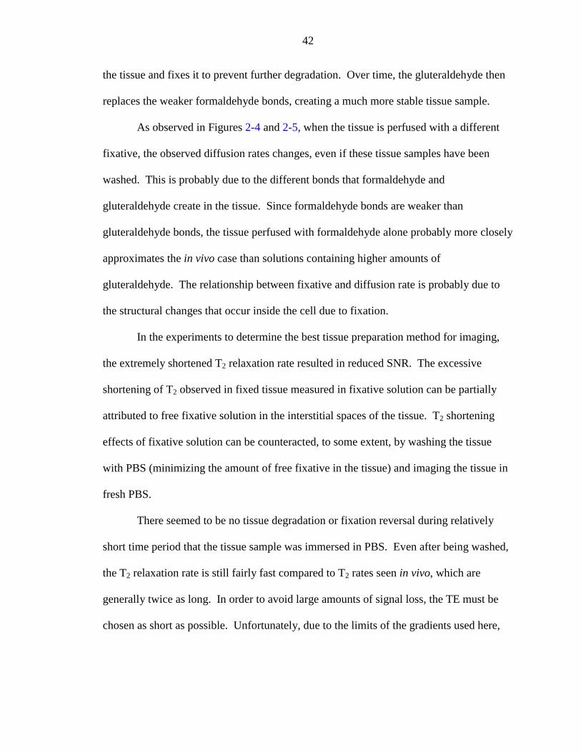
42
the tissue and fixes it to prevent further degradation. Over time, the gluteraldehyde then
replaces the weaker formaldehyde bonds, creating a much more stable tissue sample.
As observed in Figures 2-4 and 2-5, when the tissue is perfused with a different
fixative, the observed diffusion rates changes, even if these tissue samples have been
washed. This is probably due to the different bonds that formaldehyde and
gluteraldehyde create in the tissue. Since formaldehyde bonds are weaker than
gluteraldehyde bonds, the tissue perfused with formaldehyde alone probably more closely
approximates the in vivo case than solutions containing higher amounts of
gluteraldehyde. The relationship between fixative and diffusion rate is probably due to
the structural changes that occur inside the cell due to fixation.
In the experiments to determine the best tissue preparation method for imaging,
the extremely shortened T2 relaxation rate resulted in reduced SNR. The excessive
shortening of T2 observed in fixed tissue measured in fixative solution can be partially
attributed to free fixative solution in the interstitial spaces of the tissue. T2 shortening
effects of fixative solution can be counteracted, to some extent, by washing the tissue
with PBS (minimizing the amount of free fixative in the tissue) and imaging the tissue in
fresh PBS.
There seemed to be no tissue degradation or fixation reversal during relatively
short time period that the tissue sample was immersed in PBS. Even after being washed,
the T2 relaxation rate is still fairly fast compared to T2 rates seen in vivo, which are
generally twice as long. In order to avoid large amounts of signal loss, the TE must be
chosen as short as possible. Unfortunately, due to the limits of the gradients used here,
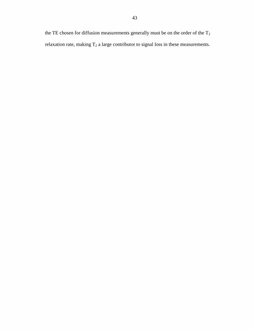
43
the TE chosen for diffusion measurements generally must be on the order of the T2
relaxation rate, making T2 a large contributor to signal loss in these measurements.

44
CHAPTER 3RELAXATION AND DIFFUSION MEASUREMENTS
ON FIXED HUMAN BRAIN SAMPLES
As seen in Chapter 1, at low diffusion gradient weightings (b �������V�PP2), the
diffusion appears to be a single diffusion rate or a single diffusion rate tensor (Fig. 1-3).
At higher gradient weightings, the data points can no longer be fitted to a single diffusion
rate or single diffusion rate tensor (Figs. 3-1 and 3-2). Instead, the data seems to be
comprised of multiple diffusion rates or a multicomponent diffusion rate tensor. Towards
the gradient limits (b §�������V�PP2), two unique diffusion components were seen in
brain and spinal cord tissue: a fast and a slow compartment. These compartments have
been ascribed to the extracellular and intracellular spaces, respectively (Karger et al.,
1988; Neindorf et al., 1996; van Zijl et al., 1991).
Data acquired by non-NMR methods have shown that the volume
fractions for the extracellular space and intracellular space is approximately 0.20 and
0.80, respectively (Nicholson & Sykova, 1998; Sykova, 1997). To test the hypothesis
that the fast component represents extracellular water and the slow component represents
intracellular water, this ratio was taken to be the standard for comparison. In the
biexponential fits (Figure 3-1 and 3-2), the volume fractions differ from the expected
volume fractions. This could be because the two compartments being visualized by
diffusion are not the extracellular and intracellular compartments, or that there are other
45
0.0 5000.0 10000.0 15000.0b value (s/mm )2
3.7
3.8
3.9
4.0
4.1
4.2
4.3
4.4
4.5
4.6
4.7
ln(S
igna
l Int
ensi
ty)
ln(Signal Intensity) vs. b valueHuman Corpus Callosum
peak height datay = 37.5exp(-0.000589b) + 62.5exp(-0.0000172b)y = 95.2exp(-0.000232b)y = 55.0exp(-0.0000162b)y = 81.3exp(-0.0000941b)
0.0 5000.0 10000.0 15000.0b values (s/mm^2)
2.2
2.4
2.6
2.8
3.0
3.2
3.4
3.6
3.8
4.0
4.2
4.4
4.6
ln(S
igna
l In
tens
ity)
ln(Signal Intensity) vs. b valueHuman Cortical Gray Matter
peak height datay = 43.3exp(-0.0004315b) + 56.7exp(0.0000290b)y = 93.8exp(-0.0001486b)y = 18.2exp(-0.0000282b)y = 39.4exp(-0.000098b)
Figure 3-1. The natural log of the signal intensity vs. b value graph for brain white matter.
Figure 3-2. The natural log of the signal intensity vs. b value graph for brain gray matter.
46
factors that effect the volume fractions calculated. Some of the parameters which may
change the observed volume fractions are relaxation weighting, in particular T2 (Chapter
2), water exchange between compartments, restriction, and proton density differences
between each compartment.
To investigate the origin of these two compartments, diffusion tensor and T2
relaxation measurements were performed with NMR spectroscopic methods on small
homogeneous samples of post-mortem, excised, fixed human corpus callosum (white
matter) and human cortical gray matter. These two samples were chosen for later
comparison with white matter and gray matter in the spinal cord. Spinal cord tissue itself
was not used because it is difficult to core a homogeneous sample from the spinal cord.
Diffusion tensor experiments were performed on these samples using echo times and
diffusion times similar to what would be used in Chapters 4 and 5 for the diffusion tensor
measurements. Also, a multiexponential measurement of T2 relaxation rates allowed the
relaxation to be taken out of the volume fractions found by the diffusion tensor
measurements.
Materials and Methods
Sample Preparation
The cadaver was flushed using a 10% formaldehyde solution, and then perfused
with a 4% solution of formaldehyde mixed with glycerin. The brain was then excised
and stored in 70% ethanol. Cylindrical sections approximately 3 mm in length and 4 mm
in diameter were cored from the corpus callosum (WM) and the cortical gray matter
(GM) of the brain. The samples were soaked in PBS for 6 hours, then sealed in a 5 mm
47
NMR tube to prevent dehydration. There was no buffer solution surrounding the tissue
samples.
NMR Measurements
1H spectra for each sample of human brain tissue were acquired on a Bruker
Avance 600 MHz spectrometer (14.1 T magnet, 54 mm bore) using a commercially
available 5 mm, three-axis, actively-shielded gradient probe capable of generating 50
G/cm per axis. The samples were maintained at 20o C throughout the NMR
measurements.
T2 relaxation measurements
T2 relaxation measurements were obtained using the Carr-Purcell-Meibloom-Gill
sequence (CPMG; see Appendix B for the sequence), with TR = 8 s and NA = 8. To
enable calculation of more than one relaxation rate, eighteen time points were taken
between TE = 2 ms and TE = 1000 ms.
Diffusion tensor measurements
ADT spectra were obtained using the method described by Basser, et al. (1992;
1994a; 1994b; Basser, 1995; Basser & Pierpaoli, 1996). For the diffusion experiments,
diffusion-weighting gradients were applied along the gradient-winding directions x, y, z,
x = y, x = z, y = z, and x = y = z. To obtain the diffusion-weighted (DW) spectra of
human brain tissue, forty different gradient weightings were applied in each direction.
Gradient strengths were chosen so that the b values would be linearly spaced between 0
and 15000 s/mm2. To acquire the spectra, the acquisition parameters were TR = 3 s, TE
= 36 ms, δ = 9 ms, ∆ = 20 ms, and NA = 4.
48
Post-Processing
T2 relaxation spectra
The peak heights of each spectrum from the T2 relaxation data were fit to a
biexponential curve of the form
( ) ( )S S TE T S TE Tij a b b= − + −0a 2 0 2exp / exp / [3-1],
where TE is the echo time, T2a(b) the long (short) relaxation times, and S0a(b) is the signal
fraction for T2a(b). As with the diffusion data, this fit was performed using a gradient-
expansion algorithm (IDL, Research Systems Incorporated).
Diffusion tensor spectra
The matrix of b values, bij (i, j = x, y, z) (Mattiello et al., 1994), was determined
for each DW spectrum in IDL. All gradient auto- and cross-terms were taken into
account with the exception of terms involving the imaging phase-encoding gradient,
which was assumed to be zero, i.e. its central value. To obtain a robust biexponential fit,
estimates of the fast and slow diffusion rates were made by separately fitting the peak
heights for the low and high ranges of b. Accordingly, the low (b = 0 to 1000 s/mm2) and
high (b = 6000 to 10000 s/mm2) diffusion-weighted series were fit to the
monoexponential curve in Eq. [1-16] using a multivariate linear regression (Montgomery,
1976). These estimated diffusion rates and the calculated relaxation rates were used as
starting points for fitting the whole data set to the biexponential curve of the form given
in Eq. [1-39], and to a biexponential curve that includes the T2 relaxation weightings:
49
( )
( )
−−+
−−=
∑∑
∑∑
i j)s(ijijb2)s(0
i j)f(ijija2)f(0
DbexpT/TEexpS
DbexpT/TEexpSS
[3-2]
where the subscripts f and s denote fast and slow components of diffusion, respectively,
and i, j = x, y, z. This fit was performed on the peak heights using a gradient-expansion
algorithm (IDL, Research Systems Incorporated, See Appendix A for examples of the
computer code).
Results
Diffusion Tensor Measurements
Figures 3-1 and 3-2 show the natural logarithm of signal intensity vs. b value for
gray matter (GM) and white matter (WM), respectively, with gradients applied along the
z direction. Table 3-1 lists the S0 and the diffusion rate values for a monoexponential fit
to the low diffusion-weighting regime (b = 0 to 1000 s/mm2), the high diffusion-
weighting regime (b = 8000 to 15000 s/mm2), the whole data set, and a biexponential fit
to the whole data set. In the high b regime, most of the signal from the fast diffusing
fraction is lost, so the diffusion rates calculated are similar to the slow component values
found by the biexponential fit. In the low b regime, however, there is a significant
contribution from both diffusion rates, so values found by monoexponential fits are
generally a factor of 2 to 3 smaller than the fast component diffusion values found by the
biexponential fit. Nevertheless, these values provide a good starting point for use in a
non-linear curve fitting routine.
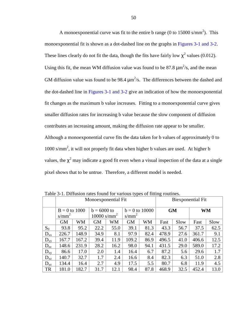
50
A monoexponential curve was fit to the entire b range (0 to 15000 s/mm2). This
monoexponential fit is shown as a dot-dashed line on the graphs in Figures 3-1 and 3-2.
These lines clearly do not fit the data, though the fits have fairly low χ2 values (0.012).
Using this fit, the mean WM diffusion value was found to be 87.8 µm2/s, and the mean
GM diffusion value was found to be 98.4 µm2/s. The differences between the dashed and
the dot-dashed line in Figures 3-1 and 3-2 give an indication of how the monoexponential
fit changes as the maximum b value increases. Fitting to a monoexponential curve gives
smaller diffusion rates for increasing b value because the slow component of diffusion
contributes an increasing amount, making the diffusion rate appear to be smaller.
Although a monoexponential curve fits the data taken for b values of approximately 0 to
1000 s/mm2, it will not properly fit data when higher b values are used. At higher b
values, the χ2 may indicate a good fit even when a visual inspection of the data at a single
pixel shows that to be untrue. Therefore, a different model is needed.
Table 3-1. Diffusion rates found for various types of fitting routines.Monoexponential Fit Biexponential Fit
B = 0 to 1000s/mm2
b = 6000 to10000 s/mm2
b = 0 to 10000s/mm2
GM WM
GM WM GM WM GM WM Fast Slow Fast SlowS0 93.8 95.2 22.2 55.0 39.1 81.3 43.3 56.7 37.5 62.5Dxx 226.7 148.9 34.9 8.1 97.9 82.4 478.9 27.6 361.7 9.1Dyy 167.7 167.2 39.4 11.9 109.2 86.9 496.5 41.0 406.6 12.5Dzz 148.6 231.9 28.2 16.2 98.0 94.1 431.5 29.0 589.0 17.2Dxy 86.6 17.0 2.0 1.4 16.4 6.7 87.2 5.6 29.6 1.7Dxz 140.7 32.7 1.7 2.4 16.6 8.4 82.3 6.3 51.0 2.8Dyz 134.4 16.4 2.7 4.9 17.5 5.5 80.7 6.8 11.9 4.5TR 181.0 182.7 31.7 12.1 98.4 87.8 468.9 32.5 452.4 13.0
51
The solid line in each graph is derived from the zero-diffusion-weighting values
(S0f and S0s) with the fast and slow Dzz values from the full tensor fit to Eq. [1-37]. The
diffusion values and zero-diffusion-weighting values found using the biexponential fit are
given in Table 3-1. The data points (Figures 3-1 and 3-2) follow the solid curves very
closely (in the x and y directions as well, not shown), indicating the biexponential fitting
routine gives an accurate fit to the tensor. For white matter, the fast component average
diffusivity (gTR, where gTR = (Dxx + Dyy + Dzz) / 3) is 452.4 µm2/s and the slow
component average diffusivity value is 13.0 µm2/s. For gray matter, the fast component
average diffusivity is 468.9 µm2/s and the slow component average diffusivity is 32.5
µm2/s. The diffusion rates found by a monoexponential fit to the entire curve are
approximately a factor of 5 smaller than the fast diffusion component, and approximately
a factor of 2.5 larger than the diffusion values found by the monoexponential fit to the
low b value regime.
The fractional contribution of fast and slow diffusion regimes to the total signal
intensity can be found by dividing each of the zero-diffusion weighting values (S0f and
S0s) by the sum of the two values. In the brain white matter, the fast component
contributes a volume fraction of approximately 0.375 and the slow component
contributes a volume fraction of approximately 0.625 to the total signal intensity. In the
brain gray matter, the fast component contributes a volume fraction of approximately
0.433 and the slow component contributes a volume fraction of approximately 0.567 to
the total signal intensity. As stated in the introduction, these differ from the expected
values of approximately 0.20 for the fast and 0.80 for the slow component. To eliminate
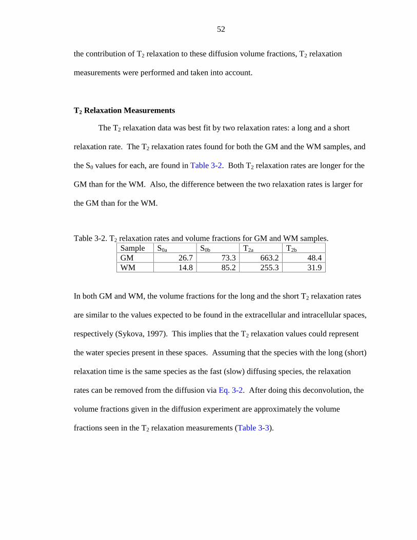
52
the contribution of T2 relaxation to these diffusion volume fractions, T2 relaxation
measurements were performed and taken into account.
T2 Relaxation Measurements
The T2 relaxation data was best fit by two relaxation rates: a long and a short
relaxation rate. The T2 relaxation rates found for both the GM and the WM samples, and
the S0 values for each, are found in Table 3-2. Both T2 relaxation rates are longer for the
GM than for the WM. Also, the difference between the two relaxation rates is larger for
the GM than for the WM.
Table 3-2. T2 relaxation rates and volume fractions for GM and WM samples.Sample S0a S0b T2a T2b
GM 26.7 73.3 663.2 48.4WM 14.8 85.2 255.3 31.9
In both GM and WM, the volume fractions for the long and the short T2 relaxation rates
are similar to the values expected to be found in the extracellular and intracellular spaces,
respectively (Sykova, 1997). This implies that the T2 relaxation values could represent
the water species present in these spaces. Assuming that the species with the long (short)
relaxation time is the same species as the fast (slow) diffusing species, the relaxation
rates can be removed from the diffusion via Eq. 3-2. After doing this deconvolution, the
volume fractions given in the diffusion experiment are approximately the volume
fractions seen in the T2 relaxation measurements (Table 3-3).
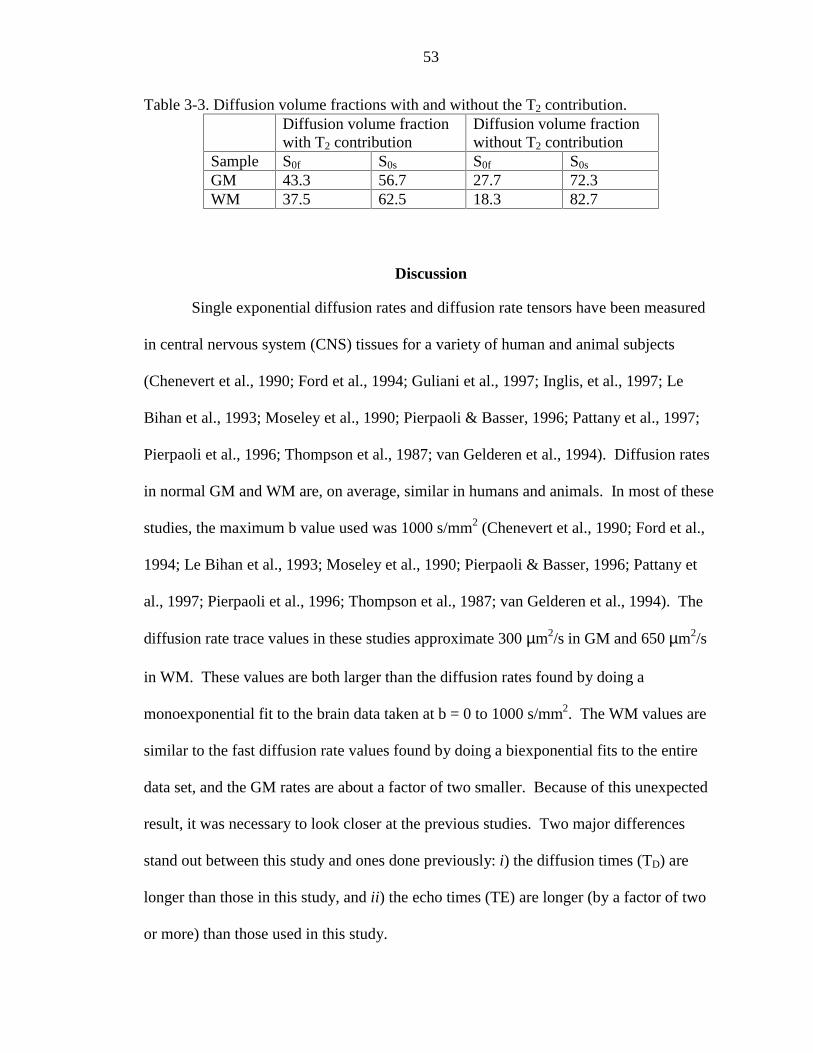
53
Table 3-3. Diffusion volume fractions with and without the T2 contribution.Diffusion volume fractionwith T2 contribution
Diffusion volume fractionwithout T2 contribution
Sample S0f S0s S0f S0s
GM 43.3 56.7 27.7 72.3WM 37.5 62.5 18.3 82.7
Discussion
Single exponential diffusion rates and diffusion rate tensors have been measured
in central nervous system (CNS) tissues for a variety of human and animal subjects
(Chenevert et al., 1990; Ford et al., 1994; Guliani et al., 1997; Inglis, et al., 1997; Le
Bihan et al., 1993; Moseley et al., 1990; Pierpaoli & Basser, 1996; Pattany et al., 1997;
Pierpaoli et al., 1996; Thompson et al., 1987; van Gelderen et al., 1994). Diffusion rates
in normal GM and WM are, on average, similar in humans and animals. In most of these
studies, the maximum b value used was 1000 s/mm2 (Chenevert et al., 1990; Ford et al.,
1994; Le Bihan et al., 1993; Moseley et al., 1990; Pierpaoli & Basser, 1996; Pattany et
al., 1997; Pierpaoli et al., 1996; Thompson et al., 1987; van Gelderen et al., 1994). The
diffusion rate trace values in these studies approximate 300 µm2/s in GM and 650 µm2/s
in WM. These values are both larger than the diffusion rates found by doing a
monoexponential fit to the brain data taken at b = 0 to 1000 s/mm2. The WM values are
similar to the fast diffusion rate values found by doing a biexponential fits to the entire
data set, and the GM rates are about a factor of two smaller. Because of this unexpected
result, it was necessary to look closer at the previous studies. Two major differences
stand out between this study and ones done previously: i) the diffusion times (TD) are
longer than those in this study, and ii) the echo times (TE) are longer (by a factor of two
or more) than those used in this study.
54
Although diffusion time may not play a significant role in the observed
differences, echo time most likely does. The T2 relaxation rate measurements done on
the brain tissue samples showed that T2 relaxation is biexponential. From the volume
fractions found here, and by observations made by others (van Dusschoten et al., 1995;
Stanisz & Henkelman, 1998), the two rates can be ascribed to the extracellular space and
the intracellular space, with the longer T2 relaxation rate being extracellular and the
shorter T2 relaxation rate being intracellular. By revisiting the assumption that the fast
diffusing species has a long T2 and the slow diffusing species have a short T2, then at
long TE the fast diffusing species will contribute more to the overall signal intensity than
the slow diffusing species. The diffusion trace rates found previously appear to support
this supposition (Chenevert et al., 1990; Ford et al., 1994; Le Bihan et al., 1993; Moseley
et al., 1990; Pierpaoli & Basser, 1996; Pattany et al., 1997; Pierpaoli et al., 1996;
Thompson et al., 1987; van Gelderen et al., 1994). The data in these experiments was
taken at echo times ranging from 70 to 110 ms. The echo times were a minimum of 2
times the short T2 relaxation rate in WM and a minimum of 1.5 times the short T2
relaxation rate in GM., So the slowly diffusing component taken at these long TE values
makes little, if any, contribution to the WM, and a slightly greater contribution to the GM
By taking the T2 relaxation time contribution out of diffusion volume fractions,
the diffusion volume fractions come close to the expected 0.20 and 0.80 for extracellular
and intracellular spaces, respectively. Since the two T2 components appear to represent
the extracellular and the intracellular spaces, and the spaces that the T2 components
represent seem to match the spaces the diffusion components represent, the diffusion
components may also represent the extracellular and intracellular compartments. Also,
55
because taking the T2 relaxation contribution away from the diffusion volume fractions
gives volume fractions close to the expected values, other mechanisms may have less of a
contribution to the changes in volume fractionation than the relaxation, at least for fixed
tissue. For example, exchange is very slow, if there is any exchange at all. So, for fixed
tissue, it may be possible to completely separate the extracellular spaces from the
intracellular spaces, making it possible to image intracellular and extracellular
compartments. In this case, the S0f and S0s images will be the relaxation-weighted images
of the extracellular and intracellular compartments, respectively, and the fast and slow
diffusion rate tensor images will show, specifically, diffusion in the extracellular and the
intracellular spaces, respectively.
56
CHAPTER 4MULTIEXPONENTIAL DIFFUSION TENSORIMAGING OF NORMAL RAT SPINAL CORD
The ability to clearly visualize normal tissue and tissue structure so that clear
comparisons can be made with injury and disease states is important. Although
histological sampling of tissue has given clear insight to both normal and pathological
tissues, such methods cannot give images of the tissue in vivo serially and over the long-
term. Though not in the detail of histology, magnetic resonance imaging can give an
overall picture of the tissue and its structure through T1-, T2-, proton density-, and
diffusion-weighted imaging. Such experiments can be done in vivo, allowing serial
measurements to be done.
The apparent diffusion tensor (ADT) can show an overall picture of tissue
structure making it useful for imaging central nervous system tissues (Basser et al.,
1994a; Basser, 1995; Basser & Pierpaoli, 1996; Chenevert et al., 1990). As we saw in
Chapter 3, however, the diffusion values found by making a single ADT map will depend
on the experimental parameters used to take the data (i.e. TE and diffusion time). This is
due to the fact that there are distinct diffusion pools within the tissue that have different
T2 relaxation rates.
Also in Chapter 3, two unique diffusion and T2 relaxation components were found
in homogeneous samples of excised, fixed human brain tissue, perhaps explaining why a
single ADT map depends on the experimental parameters. Further, evidence was seen
57
that the two components within the tissue could represent the extracellular and
intracellular compartments. Since the two diffusion components were different enough to
be separable, imaging experiments were done to visualize the two components.
Materials and Methods
Sample Preparation
A Sprague-Dawley rat was euthanized under deep general anesthesia (sodium
pentobarbital, 100 mg/kg, i.p.), exsanguinated, and perfused transcardially with
physiological (0.9%) saline followed by 4% formaldehyde solution. A 3 cm section of
spinal cord was removed from the rat (from the mid-thoracic region through the lumbar
enlargement) following euthanasia and stored in 4% formaldehyde solution.
Approximately 24 hours prior to the NMR measurements the spinal cord was rinsed in a
bath of phosphate buffered saline (PBS). Three times over the 24 hours the cord was
removed from the PBS and rinsed in a fresh bath of PBS. This procedure removed as
much of the free formaldehyde as possible from the cord since, as seen in chapter 2,
formaldehyde dramatically shortens the T2 of the sample.
Diffusion Tensor Measurements and Post Processing
Diffusion tensor measurements and post processing were done almost as
described in the previous chapter. A PGSE imaging pulse sequence was used for ADT
imaging (LeBihan and Breton, 1985). For both spectroscopy and imaging, diffusion-
weighting gradients were aligned along the gradient-winding directions x, y, z, x = y, x =
z, y = z, and x = y = z. DW-images were created used ten different gradient weightings
per direction, and were chosen so that the b values would be logarithmically spaced
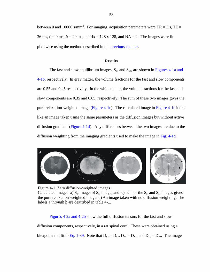
58
between 0 and 10000 s/mm2. For imaging, acquisition parameters were TR = 3 s, TE =
36 ms, δ = 9 ms, ∆ = 20 ms, matrix = 128 x 128, and NA = 2. The images were fit
pixelwise using the method described in the previous chapter.
Results
The fast and slow equilibrium images, S0f and S0s, are shown in Figures 4-1a and
4-1b, respectively. In gray matter, the volume fractions for the fast and slow components
are 0.55 and 0.45 respectively. In the white matter, the volume fractions for the fast and
slow components are 0.35 and 0.65, respectively. The sum of these two images gives the
pure relaxation-weighted image (Figure 4-1c). The calculated image in Figure 4-1c looks
like an image taken using the same parameters as the diffusion images but without active
diffusion gradients (Figure 4-1d). Any differences between the two images are due to the
diffusion weighting from the imaging gradients used to make the image in Fig. 4-1d.
Figures 4-2a and 4-2b show the full diffusion tensors for the fast and slow
diffusion components, respectively, in a rat spinal cord. These were obtained using a
biexponential fit to Eq. 1-39. Note that Dyx = Dxy, Dzx = Dxz, and Dzy = Dyz. The image
Figure 4-1. Zero diffusion-weighted images. Calculated images a) S image, b) S image, and c) sum of the S and S images gives the pure relaxation-weighted image. d) An image taken with no diffusion weighting. The labels a through h are described in table 4-1.
0f 0s 0f 0s
a b c
+ =
d a
bc
d
e
f
gh
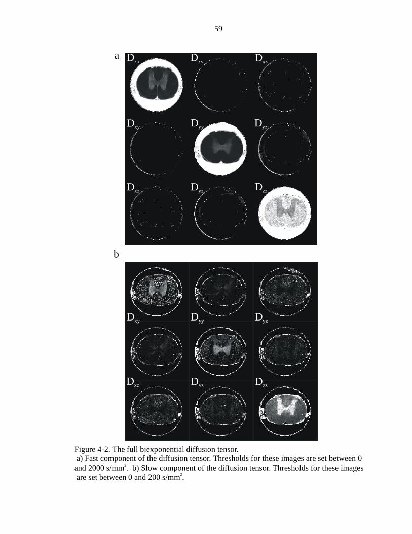
59
Dxx
Dxy
Dxy
Dyy
Dxz
Dxz
Dyz
Dyz
Dzz
a
Dxx
Dxy
Dxy
Dyy
Dxz
Dxz
Dyz
Dyz
Dzz
b
Figure 4-2. The full biexponential diffusion tensor. a) Fast component of the diffusion tensor. Thresholds for these images are set between 0 and 2000 s/mm . b) Slow component of the diffusion tensor. Thresholds for these images are set between 0 and 200 s/mm .
2
2
60
Dzz describes diffusional water motion along the length of the spinal cord (in and out of
the image plane). The image Dyy describes diffusional water motion left and right in the
image plane. The image Dxx describes diffusional water motion up and down in the
image plane. Table 4-1 contains the diffusion values for several anatomical regions of
the spinal cord. The regions chosen for Table 4-1 are numbered 1 to 8 and overlaid on
Figure 4-1d. A more complete picture of spinal cord anatomy can be found in Appendix
C.
The first noticeable difference between the fast and slow regime tensors is that the
slow regime image does not show any buffer surrounding the cord. This is expected
since free water diffusion, unlike the diffusion of water in tissue, fits a monoexponential
and does not have a slow component. The ring artifacts around the sample, noticeable in
the off-diagonal elements of the fast-diffusion tensor and in all the elements of the slow-
diffusion tensor, arise from a poor fit to regions at boundaries due to partial volume
effects.
The fast diffusion tensor (4-2a) appears as expected from the spinal cord
structure, with the white matter being oriented along the z direction (like long, thin tubes)
and the gray matter being more isotropic. The threshold in the fast diffusion trace images
is set so that the darkest points are 0 µm2/s and the brightest points are at 2000 µm2/s.
Though there is some diffusion in these elements, the off-diagonal elements appear
almost uniformly dark. This is because the diffusion rates in the off-diagonal elements
are much slower than the than their corresponding diagonal elements. The uniform
threshold values chosen to show the diagonal elements to their best advantage causes the
off-diagonal elements to disappear.
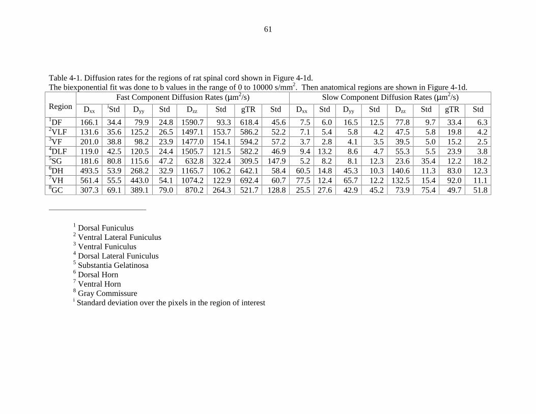
61
Table 4-1. Diffusion rates for the regions of rat spinal cord shown in Figure 4-1d.The biexponential fit was done to b values in the range of 0 to 10000 s/mm2. Then anatomical regions are shown in Figure 4-1d.
Fast Component Diffusion Rates (µm2/s) Slow Component Diffusion Rates (µm2/s)Region Dxx
iStd Dyy Std Dzz Std gTR Std Dxx Std Dyy Std Dzz Std gTR Std1DF 166.1 34.4 79.9 24.8 1590.7 93.3 618.4 45.6 7.5 6.0 16.5 12.5 77.8 9.7 33.4 6.32VLF 131.6 35.6 125.2 26.5 1497.1 153.7 586.2 52.2 7.1 5.4 5.8 4.2 47.5 5.8 19.8 4.23VF 201.0 38.8 98.2 23.9 1477.0 154.1 594.2 57.2 3.7 2.8 4.1 3.5 39.5 5.0 15.2 2.54DLF 119.0 42.5 120.5 24.4 1505.7 121.5 582.2 46.9 9.4 13.2 8.6 4.7 55.3 5.5 23.9 3.85SG 181.6 80.8 115.6 47.2 632.8 322.4 309.5 147.9 5.2 8.2 8.1 12.3 23.6 35.4 12.2 18.26DH 493.5 53.9 268.2 32.9 1165.7 106.2 642.1 58.4 60.5 14.8 45.3 10.3 140.6 11.3 83.0 12.37VH 561.4 55.5 443.0 54.1 1074.2 122.9 692.4 60.7 77.5 12.4 65.7 12.2 132.5 15.4 92.0 11.18GC 307.3 69.1 389.1 79.0 870.2 264.3 521.7 128.8 25.5 27.6 42.9 45.2 73.9 75.4 49.7 51.8
1 Dorsal Funiculus2 Ventral Lateral Funiculus3 Ventral Funiculus4 Dorsal Lateral Funiculus5 Substantia Gelatinosa6 Dorsal Horn7 Ventral Horn8 Gray Commissurei Standard deviation over the pixels in the region of interest
62
The slow diffusion tensor (Fig. 4-2b) has the threshold set such that the darkest
points are at 0 µm2/s and the brightest points are at 200 µm2/s, a factor of 10 less than
used in the fast diffusion tensor. The diffusion elements Dxx and Dyy have a similar
contrast to the fast tensor. The Dzz element, however, has contrast opposite to that seen in
the fast tensor (i.e. the GM is brighter than the WM). Table 4-1 shows explicitly that in
the fast regime, the white matter Dzz is approximately 1.4 times larger than the gray
matter Dzz, whereas in the slow regime, the gray matter Dzz is approximately 2.5 times
larger than the white matter Dzz. The relative decrease of Dzz from fast to slow is much
larger for WM than for GM. The off-diagonal elements are more obvious in the slow
diffusion tensor, but the high amount of noise in these images makes in doubtful that they
are any more significant.
Color diffusion trace (cTR) images are one method to quickly see the structural
information contained within the diffusion tensor. cTR images are not independent of the
relative orientation of the gradients to the sample, so care must be taken in orienting the
spinal cord tissue samples similarly in the magnet. The cord is placed in the gradients
such that the length of the cord (the rostral-caudal extent) is aligned with the z-axis
gradients, the lateral extent of the cord is aligned with the y-axis gradients, and the
anterior-posterior extent is aligned with the x-axis gradients. Therefore, water diffusing
in the rostral-caudal extent (i.e. in and out of the imaged plane) is defined by Dzz, water
The slow diffusion tensor (Fig. 4-2b) has the threshold set such that the darkest
points are at 0 µm2/s and the brightest points are at 200 µm2/s, a factor of 10 less than
used in the fast diffusion tensor. The diffusion elements Dxx and Dyy have a similar
contrast to the fast tensor. The Dzz element, however, has contrast opposite to that seen in
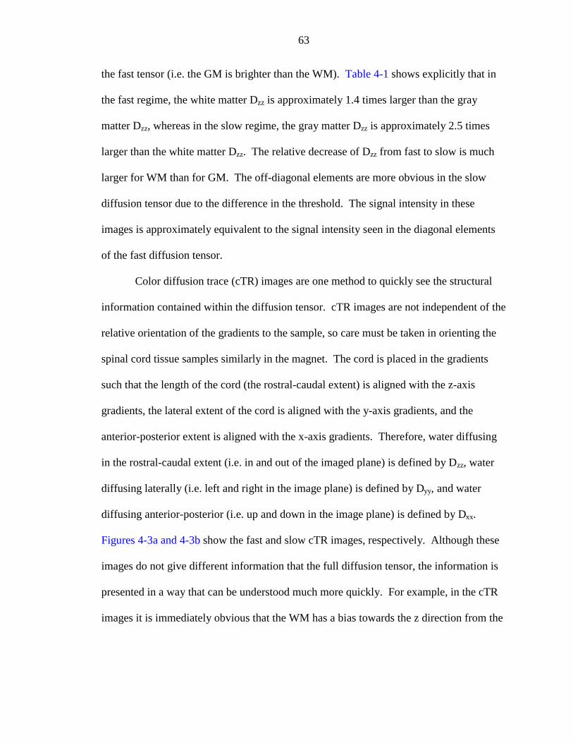
63
the fast tensor (i.e. the GM is brighter than the WM). Table 4-1 shows explicitly that in
the fast regime, the white matter Dzz is approximately 1.4 times larger than the gray
matter Dzz, whereas in the slow regime, the gray matter Dzz is approximately 2.5 times
larger than the white matter Dzz. The relative decrease of Dzz from fast to slow is much
larger for WM than for GM. The off-diagonal elements are more obvious in the slow
diffusion tensor due to the difference in the threshold. The signal intensity in these
images is approximately equivalent to the signal intensity seen in the diagonal elements
of the fast diffusion tensor.
Color diffusion trace (cTR) images are one method to quickly see the structural
information contained within the diffusion tensor. cTR images are not independent of the
relative orientation of the gradients to the sample, so care must be taken in orienting the
spinal cord tissue samples similarly in the magnet. The cord is placed in the gradients
such that the length of the cord (the rostral-caudal extent) is aligned with the z-axis
gradients, the lateral extent of the cord is aligned with the y-axis gradients, and the
anterior-posterior extent is aligned with the x-axis gradients. Therefore, water diffusing
in the rostral-caudal extent (i.e. in and out of the imaged plane) is defined by Dzz, water
diffusing laterally (i.e. left and right in the image plane) is defined by Dyy, and water
diffusing anterior-posterior (i.e. up and down in the image plane) is defined by Dxx.
Figures 4-3a and 4-3b show the fast and slow cTR images, respectively. Although these
images do not give different information that the full diffusion tensor, the information is
presented in a way that can be understood much more quickly. For example, in the cTR
images it is immediately obvious that the WM has a bias towards the z direction from the
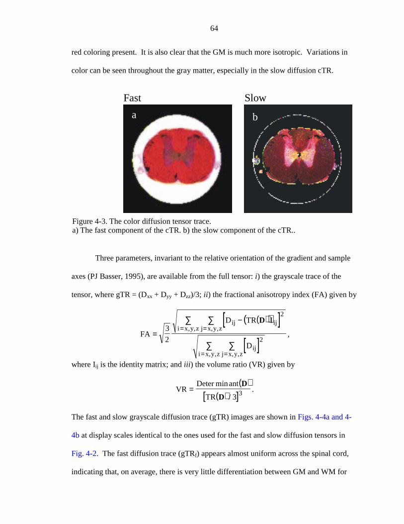
64
red coloring present. It is also clear that the GM is much more isotropic. Variations in
color can be seen throughout the gray matter, especially in the slow diffusion cTR.
Three parameters, invariant to the relative orientation of the gradient and sample
axes (PJ Basser, 1995), are available from the full tensor: i) the grayscale trace of the
tensor, where gTR = (Dxx + Dyy + Dzz)/3; ii) the fractional anisotropy index (FA) given by
( )( )[ ][ ]
FA
D TR I
D
ij ijj x y zi x y z
ijj x y zi x y z
=
−==
==
∑∑
∑∑
3
2
2
2
D, ,, ,
, ,, ,
,
where Iij is the identity matrix; and iii) the volume ratio (VR) given by
( )( )[ ]
VRDeter ant
TR=
min
/
D
D 3 3 .
The fast and slow grayscale diffusion trace (gTR) images are shown in Figs. 4-4a and 4-
4b at display scales identical to the ones used for the fast and slow diffusion tensors in
Fig. 4-2. The fast diffusion trace (gTRf) appears almost uniform across the spinal cord,
indicating that, on average, there is very little differentiation between GM and WM for
a b
Fast Slow
Figure 4-3. The color diffusion tensor trace. a) The fast component of the cTR. b) the slow component of the cTR..
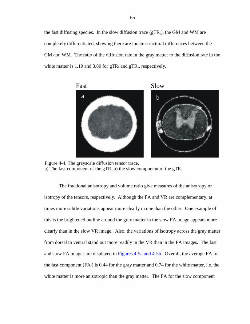
65
the fast diffusing species. In the slow diffusion trace (gTRs), the GM and WM are
completely differentiated, showing there are innate structural differences between the
GM and WM. The ratio of the diffusion rate in the gray matter to the diffusion rate in the
white matter is 1.10 and 3.80 for gTRf and gTRs, respectively.
The fractional anisotropy and volume ratio give measures of the anisotropy or
isotropy of the tensors, respectively. Although the FA and VR are complementary, at
times more subtle variations appear more clearly in one than the other. One example of
this is the brightened outline around the gray matter in the slow FA image appears more
clearly than in the slow VR image. Also, the variations of isotropy across the gray matter
from dorsal to ventral stand out more readily in the VR than in the FA images. The fast
and slow FA images are displayed in Figures 4-5a and 4-5b. Overall, the average FA for
the fast component (FAf) is 0.44 for the gray matter and 0.74 for the white matter, i.e. the
white matter is more anisotropic than the gray matter. The FA for the slow component
a b
Fast Slow
Figure 4-4. The grayscale diffusion tensor trace. a) The fast component of the gTR. b) the slow component of the gTR.
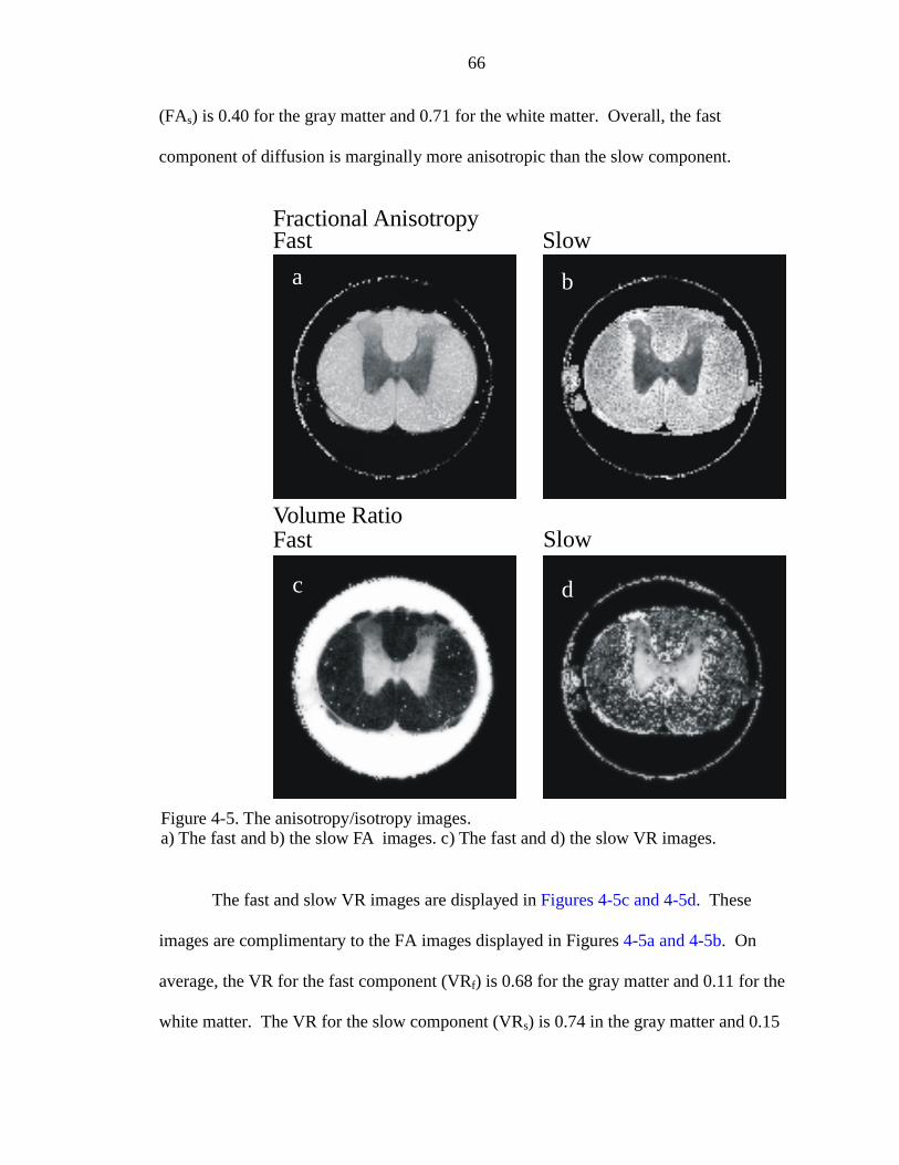
66
(FAs) is 0.40 for the gray matter and 0.71 for the white matter. Overall, the fast
component of diffusion is marginally more anisotropic than the slow component.
The fast and slow VR images are displayed in Figures 4-5c and 4-5d. These
images are complimentary to the FA images displayed in Figures 4-5a and 4-5b. On
average, the VR for the fast component (VRf) is 0.68 for the gray matter and 0.11 for the
white matter. The VR for the slow component (VRs) is 0.74 in the gray matter and 0.15
a b
Fractional AnisotropyFast Slow
c d
Fast SlowVolume Ratio
Figure 4-5. The anisotropy/isotropy images. a) The fast and b) the slow FA images. c) The fast and d) the slow VR images.
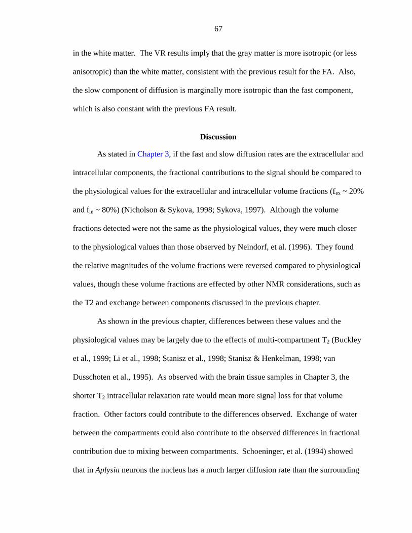
67
in the white matter. The VR results imply that the gray matter is more isotropic (or less
anisotropic) than the white matter, consistent with the previous result for the FA. Also,
the slow component of diffusion is marginally more isotropic than the fast component,
which is also constant with the previous FA result.
Discussion
As stated in Chapter 3, if the fast and slow diffusion rates are the extracellular and
intracellular components, the fractional contributions to the signal should be compared to
the physiological values for the extracellular and intracellular volume fractions (fex ~ 20%
and fin ~ 80%) (Nicholson & Sykova, 1998; Sykova, 1997). Although the volume
fractions detected were not the same as the physiological values, they were much closer
to the physiological values than those observed by Neindorf, et al. (1996). They found
the relative magnitudes of the volume fractions were reversed compared to physiological
values, though these volume fractions are effected by other NMR considerations, such as
the T2 and exchange between components discussed in the previous chapter.
As shown in the previous chapter, differences between these values and the
physiological values may be largely due to the effects of multi-compartment T2 (Buckley
et al., 1999; Li et al., 1998; Stanisz et al., 1998; Stanisz & Henkelman, 1998; van
Dusschoten et al., 1995). As observed with the brain tissue samples in Chapter 3, the
shorter T2 intracellular relaxation rate would mean more signal loss for that volume
fraction. Other factors could contribute to the differences observed. Exchange of water
between the compartments could also contribute to the observed differences in fractional
contribution due to mixing between compartments. Schoeninger, et al. (1994) showed
that in Aplysia neurons the nucleus has a much larger diffusion rate than the surrounding
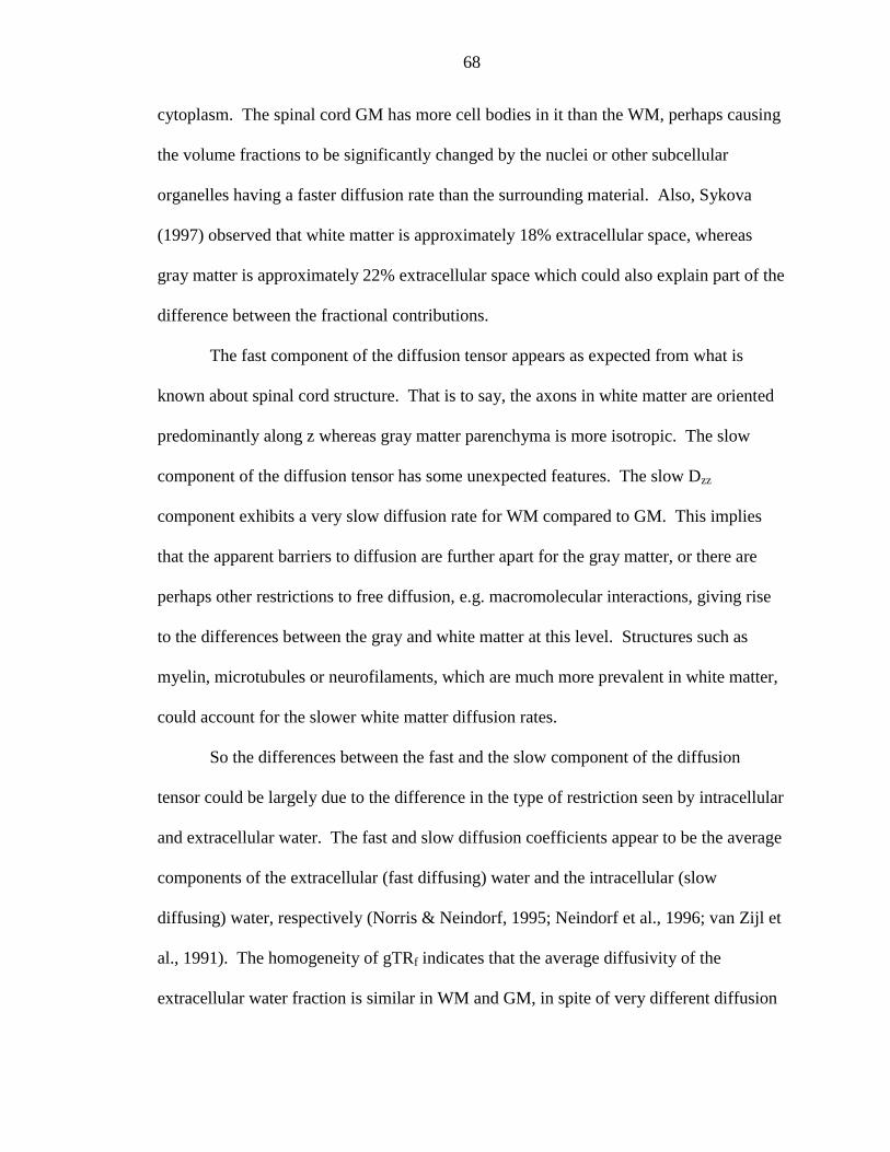
68
cytoplasm. The spinal cord GM has more cell bodies in it than the WM, perhaps causing
the volume fractions to be significantly changed by the nuclei or other subcellular
organelles having a faster diffusion rate than the surrounding material. Also, Sykova
(1997) observed that white matter is approximately 18% extracellular space, whereas
gray matter is approximately 22% extracellular space which could also explain part of the
difference between the fractional contributions.
The fast component of the diffusion tensor appears as expected from what is
known about spinal cord structure. That is to say, the axons in white matter are oriented
predominantly along z whereas gray matter parenchyma is more isotropic. The slow
component of the diffusion tensor has some unexpected features. The slow Dzz
component exhibits a very slow diffusion rate for WM compared to GM. This implies
that the apparent barriers to diffusion are further apart for the gray matter, or there are
perhaps other restrictions to free diffusion, e.g. macromolecular interactions, giving rise
to the differences between the gray and white matter at this level. Structures such as
myelin, microtubules or neurofilaments, which are much more prevalent in white matter,
could account for the slower white matter diffusion rates.
So the differences between the fast and the slow component of the diffusion
tensor could be largely due to the difference in the type of restriction seen by intracellular
and extracellular water. The fast and slow diffusion coefficients appear to be the average
components of the extracellular (fast diffusing) water and the intracellular (slow
diffusing) water, respectively (Norris & Neindorf, 1995; Neindorf et al., 1996; van Zijl et
al., 1991). The homogeneity of gTRf indicates that the average diffusivity of the
extracellular water fraction is similar in WM and GM, in spite of very different diffusion
69
anisotropies. gTRs shows that the intracellular water fraction is much more restricted for
WM than for GM, although the anisotropies are very similar to the fast diffusion regime.
These results seem due to similarities in external architecture (at least for tissue fixed
with 4% formaldehyde) for cells in each tissue type, and differences in internal cellular
architecture in each tissue type. It must be kept in mind, however, that the data was taken
at fairly long diffusion times (> 10 ms) and the two components likely cannot be
completely separated into intracellular and extracellular water due to exchange between
the compartments (Karger et al., 1988; Norris & Neindorf, 1995; Neindorf et al., 1996;
van Zijl et al., 1991).
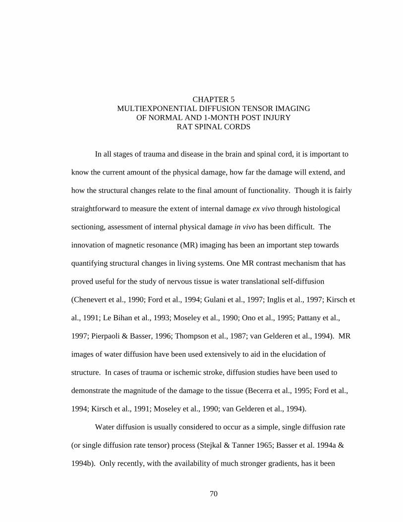
70
CHAPTER 5MULTIEXPONENTIAL DIFFUSION TENSOR IMAGING
OF NORMAL AND 1-MONTH POST INJURYRAT SPINAL CORDS
In all stages of trauma and disease in the brain and spinal cord, it is important to
know the current amount of the physical damage, how far the damage will extend, and
how the structural changes relate to the final amount of functionality. Though it is fairly
straightforward to measure the extent of internal damage ex vivo through histological
sectioning, assessment of internal physical damage in vivo has been difficult. The
innovation of magnetic resonance (MR) imaging has been an important step towards
quantifying structural changes in living systems. One MR contrast mechanism that has
proved useful for the study of nervous tissue is water translational self-diffusion
(Chenevert et al., 1990; Ford et al., 1994; Gulani et al., 1997; Inglis et al., 1997; Kirsch et
al., 1991; Le Bihan et al., 1993; Moseley et al., 1990; Ono et al., 1995; Pattany et al.,
1997; Pierpaoli & Basser, 1996; Thompson et al., 1987; van Gelderen et al., 1994). MR
images of water diffusion have been used extensively to aid in the elucidation of
structure. In cases of trauma or ischemic stroke, diffusion studies have been used to
demonstrate the magnitude of the damage to the tissue (Becerra et al., 1995; Ford et al.,
1994; Kirsch et al., 1991; Moseley et al., 1990; van Gelderen et al., 1994).
Water diffusion is usually considered to occur as a simple, single diffusion rate
(or single diffusion rate tensor) process (Stejkal & Tanner 1965; Basser et al. 1994a &
1994b). Only recently, with the availability of much stronger gradients, has it been
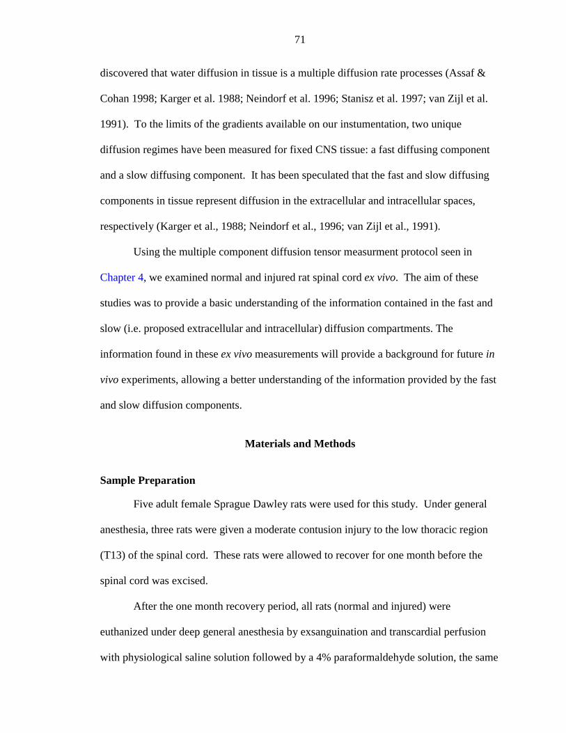
71
discovered that water diffusion in tissue is a multiple diffusion rate processes (Assaf &
Cohan 1998; Karger et al. 1988; Neindorf et al. 1996; Stanisz et al. 1997; van Zijl et al.
1991). To the limits of the gradients available on our instumentation, two unique
diffusion regimes have been measured for fixed CNS tissue: a fast diffusing component
and a slow diffusing component. It has been speculated that the fast and slow diffusing
components in tissue represent diffusion in the extracellular and intracellular spaces,
respectively (Karger et al., 1988; Neindorf et al., 1996; van Zijl et al., 1991).
Using the multiple component diffusion tensor measurment protocol seen in
Chapter 4, we examined normal and injured rat spinal cord ex vivo. The aim of these
studies was to provide a basic understanding of the information contained in the fast and
slow (i.e. proposed extracellular and intracellular) diffusion compartments. The
information found in these ex vivo measurements will provide a background for future in
vivo experiments, allowing a better understanding of the information provided by the fast
and slow diffusion components.
Materials and Methods
Sample Preparation
Five adult female Sprague Dawley rats were used for this study. Under general
anesthesia, three rats were given a moderate contusion injury to the low thoracic region
(T13) of the spinal cord. These rats were allowed to recover for one month before the
spinal cord was excised.
After the one month recovery period, all rats (normal and injured) were
euthanized under deep general anesthesia by exsanguination and transcardial perfusion
with physiological saline solution followed by a 4% paraformaldehyde solution, the same
72
procedure that was done in Chapter 4. A 3 cm section of spinal cord, centering on the
region of injury, was removed from each rat and stored in a 4% paraformaldehyde
solution. Approximately 24 hours prior to NMR measurement, the spinal cords were
placed in a bath of phosphate buffered saline (PBS). These cords were placed in fresh
baths of PBS three more times before being inserted into the magnet. This procedure was
done to remove as much free paraformaldehyde as possible from the cord since free
paraformaldehyde in the solution surrounding the tissue will dramatically shorten the T2
relaxation rate of the sample as seen in Chapter 2.
NMR Experiments
Magnetic resonance microscopy and diffusion measurements were performed on
all rat spinal cords using a Varian Unity 600 spectrometer (14.1 T magnet, 51 mm bore).
The gradient probe used was a 5 mm radio-frequency coil, three-axis actively-shielded
Varian gradient probe capable of 300 mT m-1 per axis. Sample temperature was
maintained at 200 C through the entire measurement protocol. The microimaging
measurements were performed using a pulsed gradient spin echo (PGSE) sequence.
Images of the spinal cords were taken in contiguous 250 µm thick transverse slices.
Other acquisition parameters included TR = 8 s, TE = 14 ms, and a matrix of 256 x 256.
Overall measurement time was 1.5 hours.
The ADT imaging procedure used for the spinal cord was adapted from that
described by Basser, et al. (1994a & 1994b), the same procedure that was utilized in
Chapter 4. Diffusion-weighted (DW) images were acquired using a PGSE imaging
sequence with diffusion gradients aligned along the directions x, y, z, x = y, x = z, y = z
and x = y = z. Ten gradient weightings were applied in each direction to give b values
73
that were approximately logarithmically spaced between 0 and 10000 s/mm2. Other
acquisition parameters included TR = 3 s, TE = 36 ms, δ = 9 ms, ∆ = 20 ms, matrix = 64
x 64 and NA = 4. The in-plane resolution was 78 µm x 78 µm and the slice thickness
was 1.0 mm. The overall measurement time was 16 hours.
For each cord, three sets of diffusion and microimaging experiments were done.
One set (6 diffusion slices) was at the epicenter of injury. One set was rostral to the
epicenter (with slice 6 of this set being the same as slice 1 of the epicenter set). The third
set was caudal to the epicenter of injury (with slice 1 of this set being the same as slice 6
of the epicenter set). This procedure allowed for 16 diffusion slices to be made through
the spinal cord, allowing the visualization of damage to the cord as much as 7-8 mm
rostrally and caudally.
Results
Figures 5-1 to 5-3 show diffusion trace images for both normal and 1-month post-
injury rat spinal cords. Self-diffusion in the spinal cord is given in the coordinate system
of the gradient axes. The gTR images (b, d, f and h in Figs. 5-1, 5-2 and 5-3) give an
average diffusion rate across the cord that is independent of the cord orientation. As in
Chapter 4, the cTR images (a, c, e and g in Figs. 5-1, 5-2 and 5-3), in which red indicates
Dzz, green indicates Dyy, and blue indicates Dxx are not independent of cord orientation
inside the gradients. Although the cTR is not independent of cord orientation, all the
tissue samples were equivalently aligned within the gradients so that the cTR images
from different cords could be compared. The cTR images show some structural
differences more readily than the gTR images.
74
Normal Injured
a
b
e
f
FastColor Diffusion Trace
c
d
g
h
SlowColor Diffusion Trace
Grayscale Diffusion Trace
Grayscale Diffusion Trace
Figure 5-1. Diffusion trace images 7 mm rostral to the epicenter of injury. Fast component of the a) cTR and b) gTR; slow component of the c) cTR and d) gTR for normal rat spinal cord. Fast component of the e) cTR and f) gTR; slow component of the g) cTR and h) gTR for a rat spinal cord 1-month post injury.
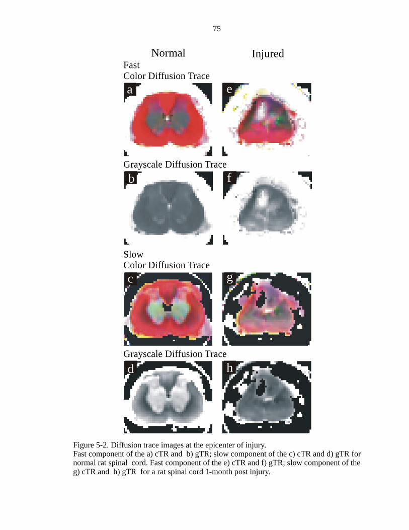
75
Figure 5-2. Diffusion trace images at the epicenter of injury. Fast component of the a) cTR and b) gTR; slow component of the c) cTR and d) gTR for normal rat spinal cord. Fast component of the e) cTR and f) gTR; slow component of the g) cTR and h) gTR for a rat spinal cord 1-month post injury.
ea
b
c
d
f
g
h
Normal InjuredFastColor Diffusion Trace
Grayscale Diffusion Trace
SlowColor Diffusion Trace
Grayscale Diffusion Trace
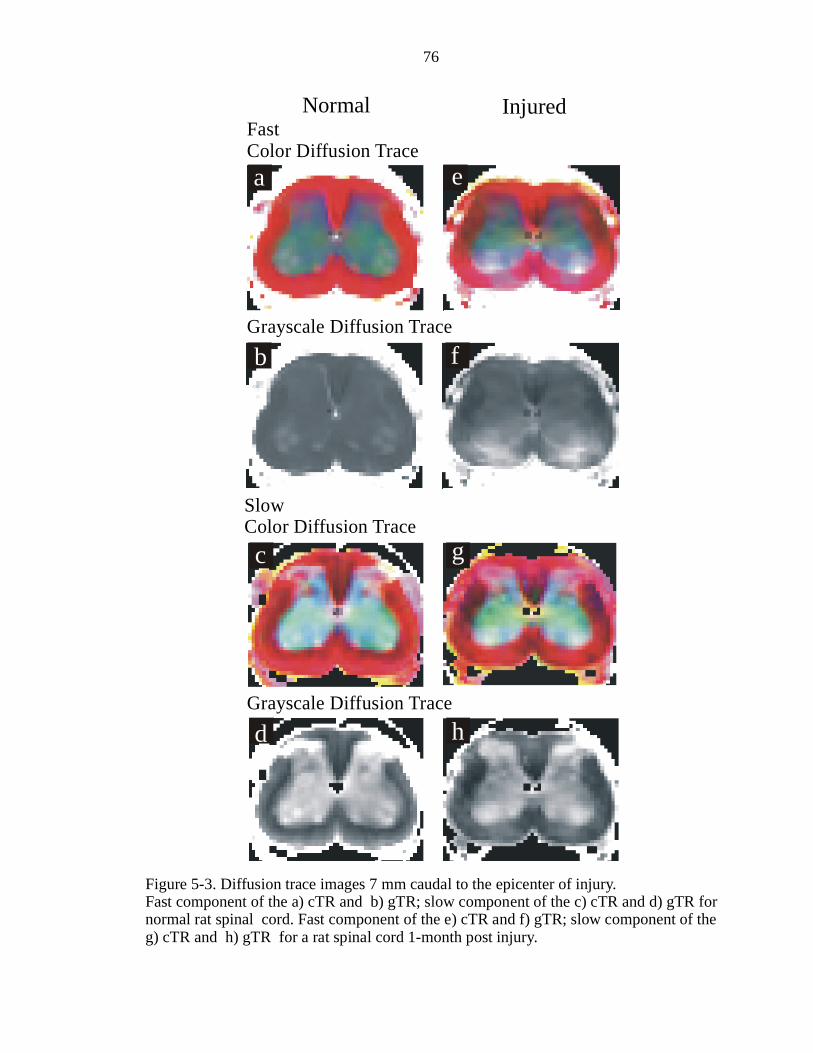
76
Figure 5-3. Diffusion trace images 7 mm caudal to the epicenter of injury. Fast component of the a) cTR and b) gTR; slow component of the c) cTR and d) gTR for normal rat spinal cord. Fast component of the e) cTR and f) gTR; slow component of the g) cTR and h) gTR for a rat spinal cord 1-month post injury.
ea
b f
c g
d h
Normal InjuredFastColor Diffusion Trace
Grayscale Diffusion Trace
SlowColor Diffusion Trace
Grayscale Diffusion Trace
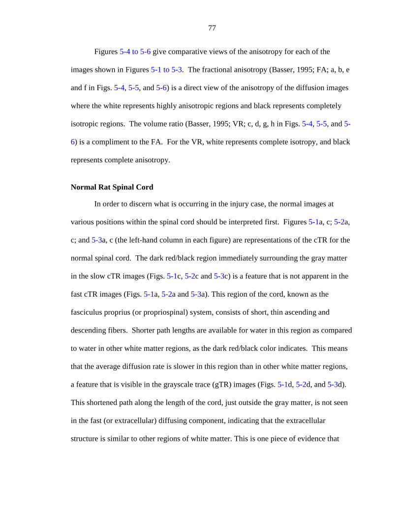
77
Figures 5-4 to 5-6 give comparative views of the anisotropy for each of the
images shown in Figures 5-1 to 5-3. The fractional anisotropy (Basser, 1995; FA; a, b, e
and f in Figs. 5-4, 5-5, and 5-6) is a direct view of the anisotropy of the diffusion images
where the white represents highly anisotropic regions and black represents completely
isotropic regions. The volume ratio (Basser, 1995; VR; c, d, g, h in Figs. 5-4, 5-5, and 5-
6) is a compliment to the FA. For the VR, white represents complete isotropy, and black
represents complete anisotropy.
Normal Rat Spinal Cord
In order to discern what is occurring in the injury case, the normal images at
various positions within the spinal cord should be interpreted first. Figures 5-1a, c; 5-2a,
c; and 5-3a, c (the left-hand column in each figure) are representations of the cTR for the
normal spinal cord. The dark red/black region immediately surrounding the gray matter
in the slow cTR images (Figs. 5-1c, 5-2c and 5-3c) is a feature that is not apparent in the
fast cTR images (Figs. 5-1a, 5-2a and 5-3a). This region of the cord, known as the
fasciculus proprius (or propriospinal) system, consists of short, thin ascending and
descending fibers. Shorter path lengths are available for water in this region as compared
to water in other white matter regions, as the dark red/black color indicates. This means
that the average diffusion rate is slower in this region than in other white matter regions,
a feature that is visible in the grayscale trace (gTR) images (Figs. 5-1d, 5-2d, and 5-3d).
This shortened path along the length of the cord, just outside the gray matter, is not seen
in the fast (or extracellular) diffusing component, indicating that the extracellular
structure is similar to other regions of white matter. This is one piece of evidence that
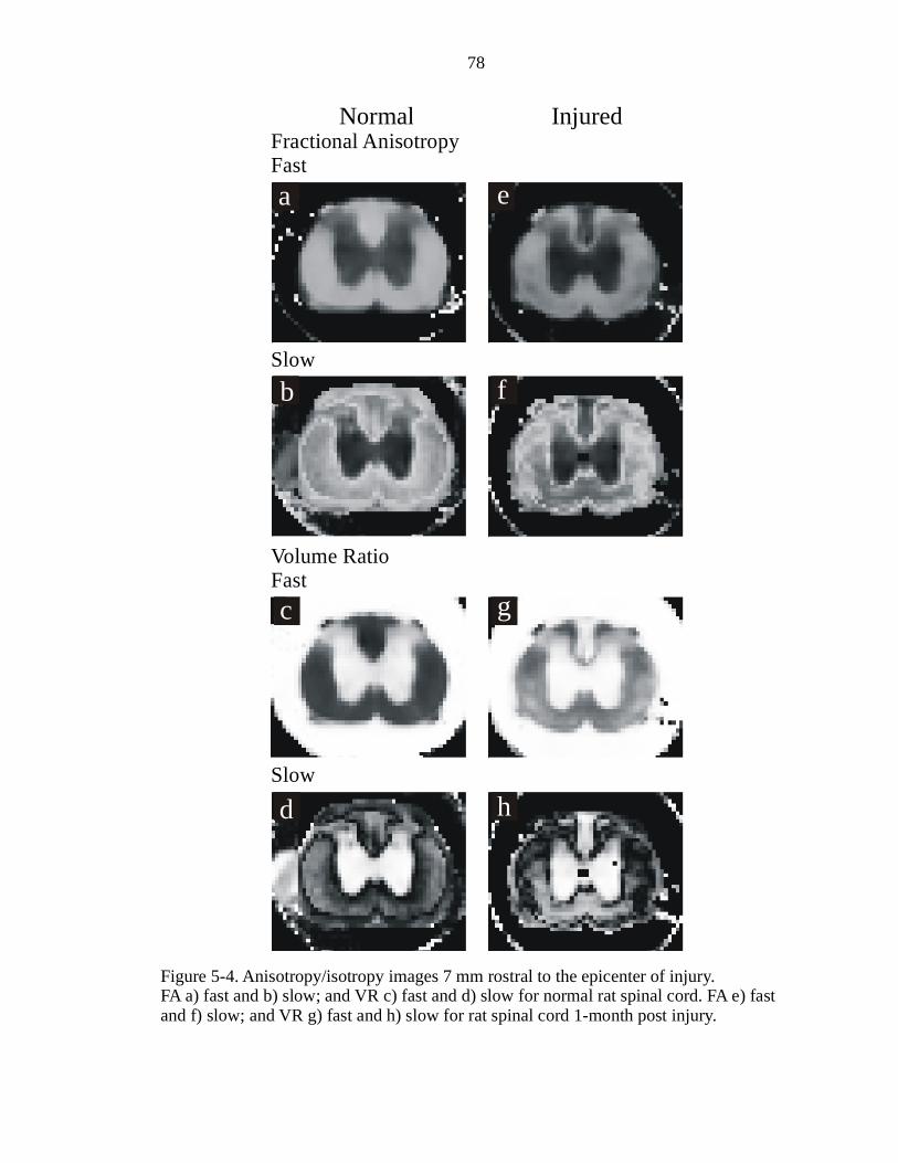
78
Figure 5-4. Anisotropy/isotropy images 7 mm rostral to the epicenter of injury. FA a) fast and b) slow; and VR c) fast and d) slow for normal rat spinal cord. FA e) fast and f) slow; and VR g) fast and h) slow for rat spinal cord 1-month post injury.
Normal Injured
a e
Fractional AnisotropyFast
b fSlow
c g
Volume RatioFast
d hSlow
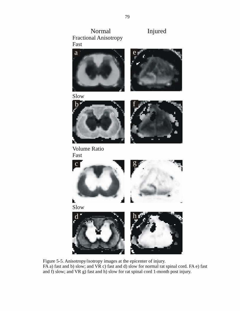
79
Figure 5-5. Anisotropy/isotropy images at the epicenter of injury. FA a) fast and b) slow; and VR c) fast and d) slow for normal rat spinal cord. FA e) fast and f) slow; and VR g) fast and h) slow for rat spinal cord 1-month post injury.
e
f
g
h
a
b
c
dSlow
Volume RatioFast
Slow
Normal InjuredFractional AnisotropyFast
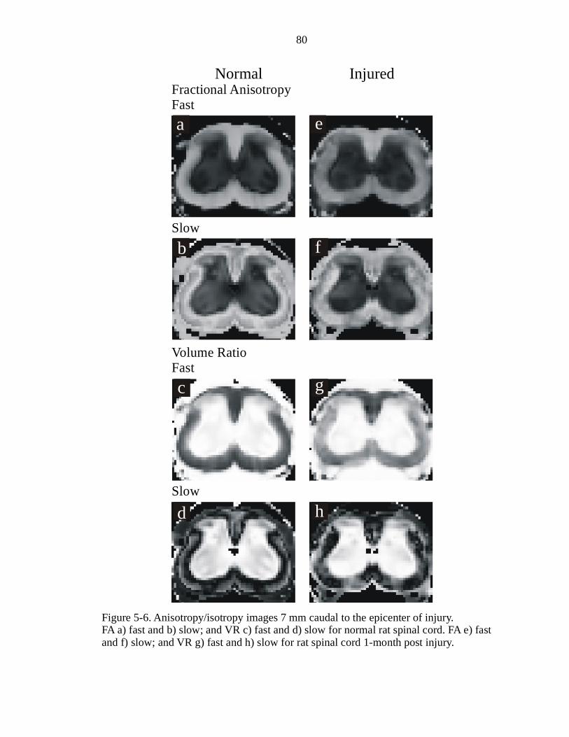
80
Figure 5-6. Anisotropy/isotropy images 7 mm caudal to the epicenter of injury. FA a) fast and b) slow; and VR c) fast and d) slow for normal rat spinal cord. FA e) fast and f) slow; and VR g) fast and h) slow for rat spinal cord 1-month post injury.
a
b
c
d
e
f
g
h
Normal InjuredFractional AnisotropyFast
Slow
Volume RatioFast
Slow
81
seems to confirm the proposition that the two components of diffusion represent the
extracellular (fast) and intracellular (slow) compartments.
For the fast component, the graph of the diffusion trace values vs. slice position
(Fig. 5-7a) shows that the average diffusion rate in the gray matter regions is slightly
higher than the average diffusion rate in the white matter regions. This information leads
to the conclusion that, on average, if the fast component corresponds to water diffusion in
the extracellular space, the rate of diffusion is similar for both gray and white matter.
This would be expected since the extracellular matrix should be similar. For the slow
component, the graph of the diffusion trace values vs. slice position (Fig. 5-7b) shows
that the average diffusion rate in the gray matter regions is approximately two times
faster than the average diffusion rate in the white matter regions. This difference may be
reflective of the difference in internal structure of the gray and white matter, where gray
matter is composed of mostly cell bodies and white matter is composed mostly of axons.
In the fast cTR images (Figs. 5-1a, 5-2a and 5-3a), the majority of the gray matter
regions appear to be varying shades of blue/green to yellow/gray, reflecting the more
isotropic nature of the extracellular spaces in the gray matter. Variations in the color
appear to coincide with the variation in the differing cell types occurring in each gray
matter lamina. These variations are enhanced in the slow cTR images (Figs. 5-1c, 5-2c
and 5-3c) where the gray matter appears in more distinct shades of green, blue and red,
reflecting the orientation of cell bodies and fibers, as well as different internal cell
structure, for each lamina.
From the FA and VR images (a, b, c and d in Figs. 5-4, 5-5, and 5-6), as well as
the graphical representations of each (a and b in Figs. 5-8 and 5-9), gray matter is much
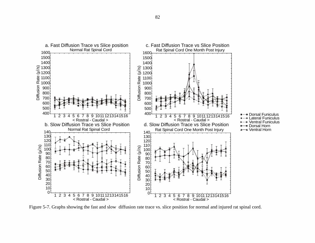
82
1 2 3 4 5 6 7 8 9 10111213141516< Rostral - Caudal >
400500600700800900
1000110012001300140015001600
Diff
usio
n R
ate
(/s
)µ2
a. Fast Diffusion Trace vs Slice positionNormal Rat Spinal Cord
1 2 3 4 5 6 7 8 9 10111213141516< Rostral - Caudal >
400500600700800900
1000110012001300140015001600
Diff
usio
n R
ate
(/s
)µ2
c. Fast Diffusion Trace vs Slice PositionRat Spinal Cord One Month Post Injury
1 2 3 4 5 6 7 8 9 10111213141516< Rostral - Caudal >
0102030405060708090
100110120130140
Diff
usio
n R
ate
(/s
)µ2
b. Slow Diffusion Trace vs Slice PositionNormal Rat Spinal Cord
1 2 3 4 5 6 7 8 9 1011 1213141516< Rostral - Caudal >
0102030405060708090
100110120130140
Diff
usio
n R
ate
(/s
)µ2
d. Slow Diffusion Trace vs Slice PositionRat Spinal Cord One Month Post Injury
Dorsal Funiculus
Dorsal Horn
Lateral FuniculusVentral Funiculus
Ventral Horn
Figure 5-7. Graphs showing the fast and slow diffusion rate trace vs. slice position for normal and injured rat spinal cord.
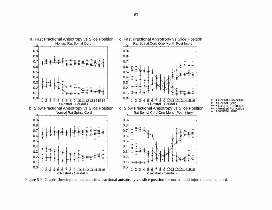
83
Figure 5-8. Graphs showing the fast and slow fractional anisotropy vs. slice position for normal and injured rat spinal cord.
1 2 3 4 5 6 7 8 9 10111213141516< Rostral - Caudal >
0.0
0.1
0.2
0.3
0.4
0.5
0.6
0.7
0.8
0.9
1.0
a. Fast Fractional Anisotropy vs Slice PositionNormal Rat Spinal Cord
1 2 3 4 5 6 7 8 9 1011 1213141516< Rostral - Caudal >
0.0
0.1
0.2
0.3
0.4
0.5
0.6
0.7
0.8
0.9
1.0
b. Slow Fractional Anisotropy vs Slice PositionNormal Rat Spinal Cord
1 2 3 4 5 6 7 8 9 1011 1213141516< Rostral - Caudal >
0.0
0.1
0.2
0.3
0.4
0.5
0.6
0.7
0.8
0.9
1.0
d. Slow Fractional Anisotropy vs Slice PositionRat Spinal Cord One Month Post Injury
< Rostral - Caudal >1 2 3 4 5 6 7 8 9 10111213141516
0.0
0.1
0.2
0.3
0.4
0.5
0.6
0.7
0.8
0.9
1.0
c. Fast Fractional Anisotropy vs Slice PositionRat Spinal Cord One Month Post Injury
Dorsal FuniculusDorsal HornLateral FuniculusVentral FuniculusVentral Horn
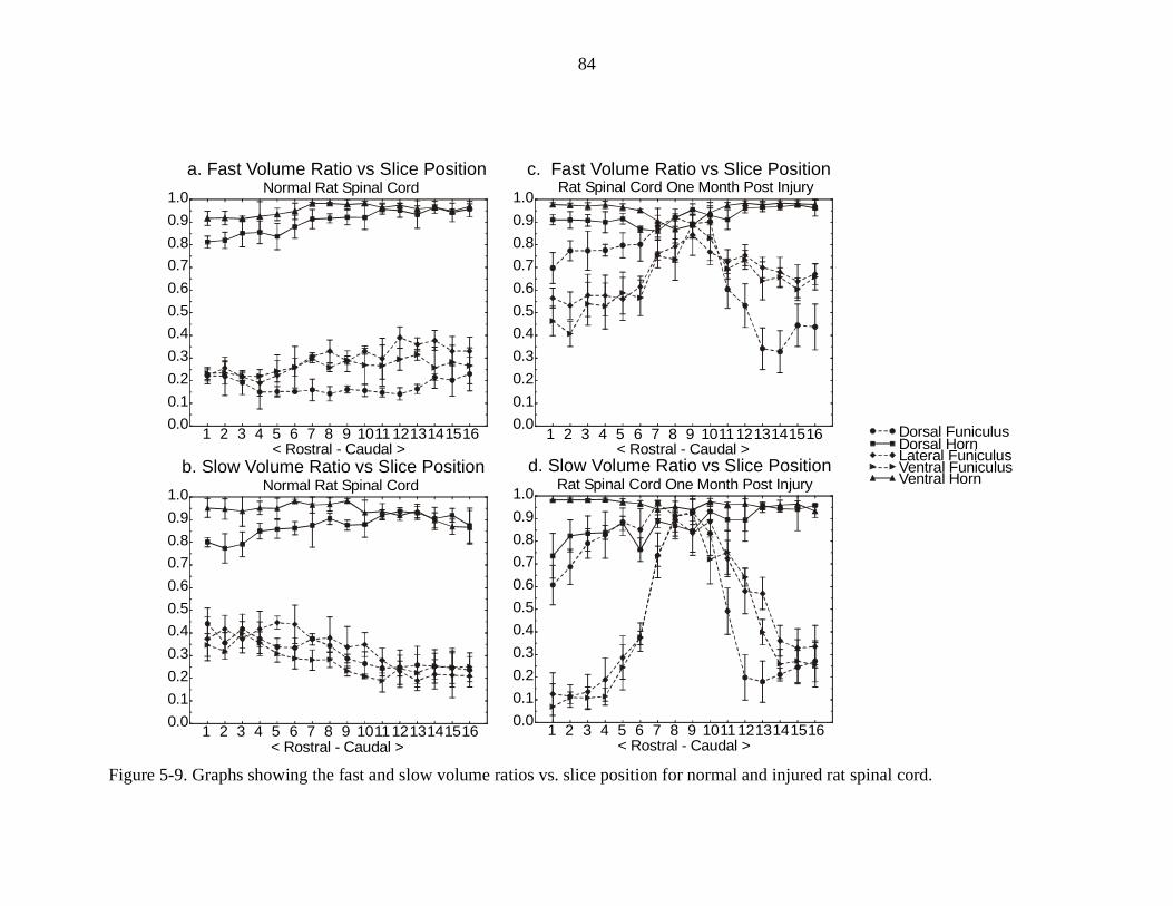
84
Figure 5-9. Graphs showing the fast and slow volume ratios vs. slice position for normal and injured rat spinal cord.
Dorsal FuniculusDorsal HornLateral FuniculusVentral FuniculusVentral Horn
1 2 3 4 5 6 7 8 9 1011 1213141516< Rostral - Caudal >
0.0
0.1
0.2
0.3
0.4
0.5
0.6
0.7
0.8
0.9
1.0
a. Fast Volume Ratio vs Slice PositionNormal Rat Spinal Cord
1 2 3 4 5 6 7 8 9 10111213141516< Rostral - Caudal >
0.0
0.1
0.2
0.3
0.4
0.5
0.6
0.7
0.8
0.9
1.0
b. Slow Volume Ratio vs Slice PositionNormal Rat Spinal Cord
1 2 3 4 5 6 7 8 9 1011 1213141516< Rostral - Caudal >
0.0
0.1
0.2
0.3
0.4
0.5
0.6
0.7
0.8
0.9
1.0
d. Slow Volume Ratio vs Slice PositionRat Spinal Cord One Month Post Injury
1 2 3 4 5 6 7 8 9 10111213141516< Rostral - Caudal >
0.0
0.1
0.2
0.3
0.4
0.5
0.6
0.7
0.8
0.9
1.0
c. Fast Volume Ratio vs Slice PositionRat Spinal Cord One Month Post Injury
85
more isotropic than white matter in all regions of the cord for both the fast and the slow
diffusing components. Rostral to caudal in the sixteen slices of the rat spinal cord, the
fast diffusing species in the gray matter becomes slightly more isotropic in all regions.
Rostral to caudal in the sixteen slices of the rat spinal cord, the slow diffusing species in
the dorsal gray matter becomes slightly more isotropic down the length of the cord, but
ventral gray matter becomes slightly more anisotropic. These variations probably reflect
the changes in structure of the gray matter in various parts of the spinal cord. However,
the white matter has almost no variation in its diffusion isotropy across these sixteen
slices. This is seen in the graphs of FA and VR, as well as in the images in the three
regions: for FA the white matter always appears almost white, and in the VR it appears
the same shade of dark gray. Moving rostral to caudal, the major differences in white
matter are the relative proportions of ascending to descending fibers, but there are few, if
any, differences between the structure of ascending and descending fibers beyond the
location of the main cell body. Therefore, it seems reasonable that the diffusion isotropy
in white matter would not change significantly, but that the diffusion isotropy in gray
matter might change along the length of a normal rat spinal cord.
Rat Spinal Cord 1-Month Post Injury
With a basic understanding of the structures and structural differences seen with
diffusion tensor imaging of the normal cord, the injured cord data can be interpreted.
First, the fasciculus proprius may no longer be easily discerned in the cTR and gTR
images of the slowly diffusing component (Figs. 5-1g, 5-1h, 5-2g, 5-2h, 5-3g and 5-3h).
It has become less differentiated from the surrounding white matter because the
surrounding white matter has, in general, become more isotropic and exhibits slower
86
diffusion rates. There should be some amount of disruptions inside the axons due to
degeneration and apoptosis, where internal cellular structures are breaking apart; or cell
survival strategies, where cells produce more organelles in an effort to survive. These
changes would cause slower diffusion rates to occur in the long white matter axons,
making them indistinguishable from the propriospinal regions of the cord.
Epicenter of injury
At the epicenter of injury, it is clear that there are major changes (Figs. 5-2e-h and
5-5e-h). A fluid filled cavity has appeared in the cord. Diffusion in the remaining white
matter tissue is much more isotropic, particularly in the dorsal and lateral sections of the
cord. This is seen in the FA (Figs. 5-5e, f) and VR images (Figs. 5-5g, h) as well as in
the FA or VR vs. slice position graphs (Figs 5-8 and 5-9). In the most ventral portion of
the cord, the fast component appears to be more anisotropic, and thus the tissue appears
more structured than the rest of the cord. This is indicative of spared white matter in this
region. The slow component of diffusion in that same region appears more isotropic,
which is more consistent with the rest of the cord. Gray matter regions are, on average,
slightly more anisotropic than normal for the fast diffusing species and slightly more
isotropic than normal for the slow diffusing species. Slices 5-8 and 5-9 (epicenter of the
injury) in the graphs of the diffusion trace vs. slice position (Fig. 5-7) show that the fast
diffusion rate is faster than in normal tissue, approaching that of free water, for all
regions of the cord. The slow diffusion rate, however, is slower than in normal tissue for
the gray matter regions, but appears almost normal for the white matter regions. The
quicker than normal rate of diffusion for the fast compartment could indicate a rising
amount of free space due to surrounding cellular damage and death, dissolution of the
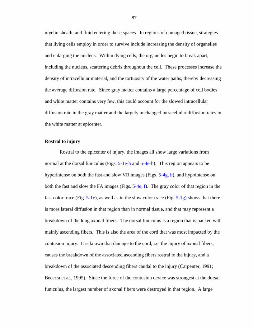
87
myelin sheath, and fluid entering these spaces. In regions of damaged tissue, strategies
that living cells employ in order to survive include increasing the density of organelles
and enlarging the nucleus. Within dying cells, the organelles begin to break apart,
including the nucleus, scattering debris throughout the cell. These processes increase the
density of intracellular material, and the tortuosity of the water paths, thereby decreasing
the average diffusion rate. Since gray matter contains a large percentage of cell bodies
and white matter contains very few, this could account for the slowed intracellular
diffusion rate in the gray matter and the largely unchanged intracellular diffusion rates in
the white matter at epicenter.
Rostral to injury
Rostral to the epicenter of injury, the images all show large variations from
normal at the dorsal funiculus (Figs. 5-1e-h and 5-4e-h). This region appears to be
hyperintense on both the fast and slow VR images (Figs. 5-4g, h), and hypointense on
both the fast and slow the FA images (Figs. 5-4e, f). The gray color of that region in the
fast color trace (Fig. 5-1e), as well as in the slow color trace (Fig. 5-1g) shows that there
is more lateral diffusion in that region than in normal tissue, and that may represent a
breakdown of the long axonal fibers. The dorsal funiculus is a region that is packed with
mainly ascending fibers. This is also the area of the cord that was most impacted by the
contusion injury. It is known that damage to the cord, i.e. the injury of axonal fibers,
causes the breakdown of the associated ascending fibers rostral to the injury, and a
breakdown of the associated descending fibers caudal to the injury (Carpenter, 1991;
Becerra et al., 1995). Since the force of the contusion device was strongest at the dorsal
funiculus, the largest number of axonal fibers were destroyed in that region. A large
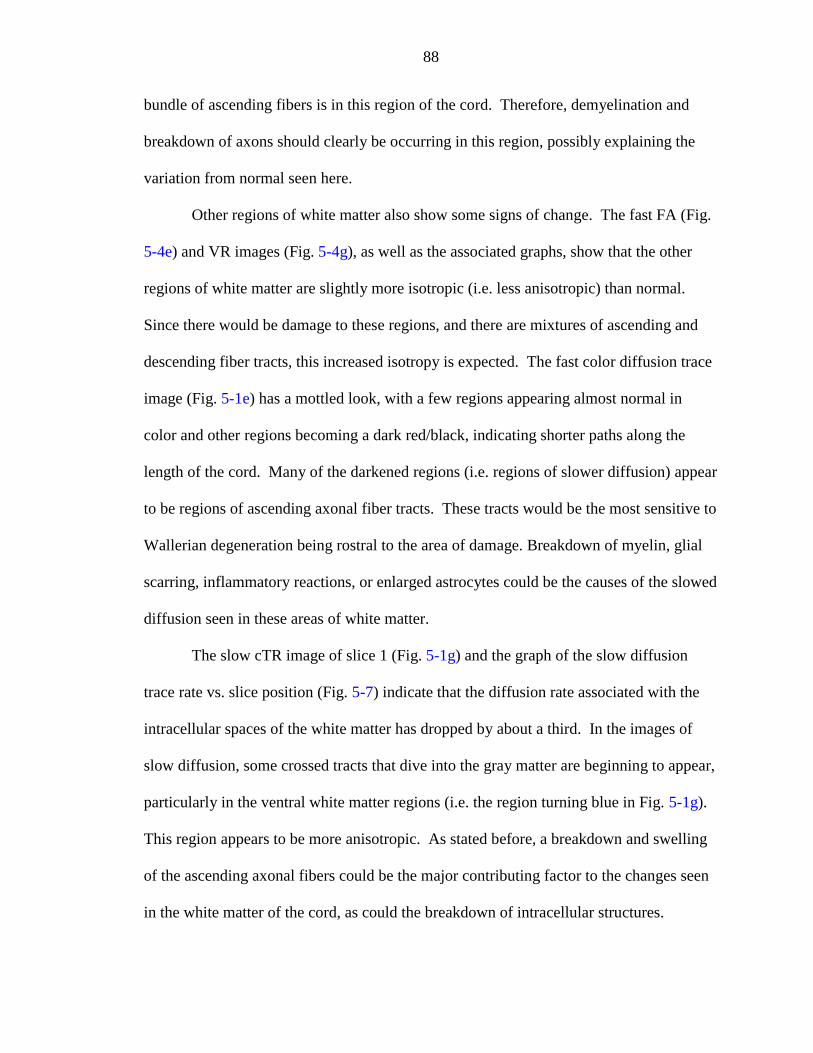
88
bundle of ascending fibers is in this region of the cord. Therefore, demyelination and
breakdown of axons should clearly be occurring in this region, possibly explaining the
variation from normal seen here.
Other regions of white matter also show some signs of change. The fast FA (Fig.
5-4e) and VR images (Fig. 5-4g), as well as the associated graphs, show that the other
regions of white matter are slightly more isotropic (i.e. less anisotropic) than normal.
Since there would be damage to these regions, and there are mixtures of ascending and
descending fiber tracts, this increased isotropy is expected. The fast color diffusion trace
image (Fig. 5-1e) has a mottled look, with a few regions appearing almost normal in
color and other regions becoming a dark red/black, indicating shorter paths along the
length of the cord. Many of the darkened regions (i.e. regions of slower diffusion) appear
to be regions of ascending axonal fiber tracts. These tracts would be the most sensitive to
Wallerian degeneration being rostral to the area of damage. Breakdown of myelin, glial
scarring, inflammatory reactions, or enlarged astrocytes could be the causes of the slowed
diffusion seen in these areas of white matter.
The slow cTR image of slice 1 (Fig. 5-1g) and the graph of the slow diffusion
trace rate vs. slice position (Fig. 5-7) indicate that the diffusion rate associated with the
intracellular spaces of the white matter has dropped by about a third. In the images of
slow diffusion, some crossed tracts that dive into the gray matter are beginning to appear,
particularly in the ventral white matter regions (i.e. the region turning blue in Fig. 5-1g).
This region appears to be more anisotropic. As stated before, a breakdown and swelling
of the ascending axonal fibers could be the major contributing factor to the changes seen
in the white matter of the cord, as could the breakdown of intracellular structures.
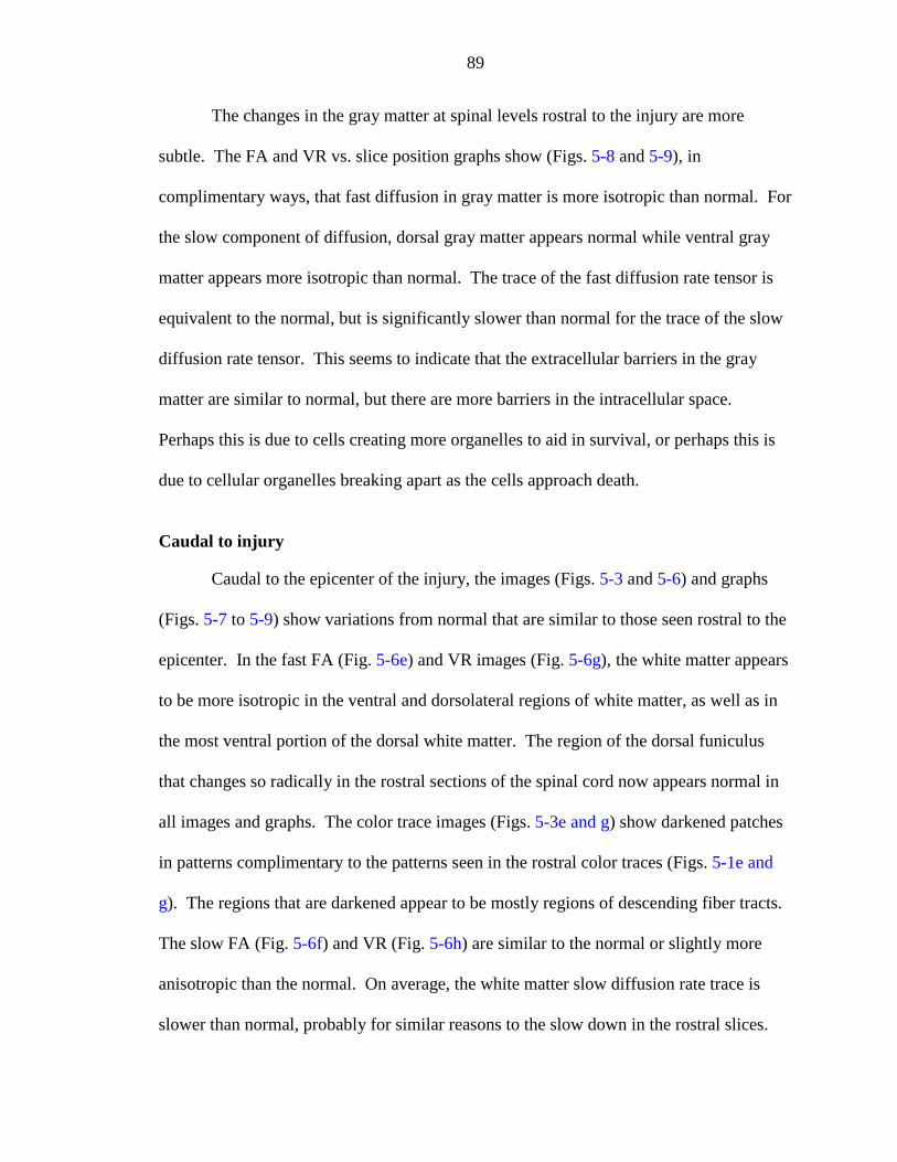
89
The changes in the gray matter at spinal levels rostral to the injury are more
subtle. The FA and VR vs. slice position graphs show (Figs. 5-8 and 5-9), in
complimentary ways, that fast diffusion in gray matter is more isotropic than normal. For
the slow component of diffusion, dorsal gray matter appears normal while ventral gray
matter appears more isotropic than normal. The trace of the fast diffusion rate tensor is
equivalent to the normal, but is significantly slower than normal for the trace of the slow
diffusion rate tensor. This seems to indicate that the extracellular barriers in the gray
matter are similar to normal, but there are more barriers in the intracellular space.
Perhaps this is due to cells creating more organelles to aid in survival, or perhaps this is
due to cellular organelles breaking apart as the cells approach death.
Caudal to injury
Caudal to the epicenter of the injury, the images (Figs. 5-3 and 5-6) and graphs
(Figs. 5-7 to 5-9) show variations from normal that are similar to those seen rostral to the
epicenter. In the fast FA (Fig. 5-6e) and VR images (Fig. 5-6g), the white matter appears
to be more isotropic in the ventral and dorsolateral regions of white matter, as well as in
the most ventral portion of the dorsal white matter. The region of the dorsal funiculus
that changes so radically in the rostral sections of the spinal cord now appears normal in
all images and graphs. The color trace images (Figs. 5-3e and g) show darkened patches
in patterns complimentary to the patterns seen in the rostral color traces (Figs. 5-1e and
g). The regions that are darkened appear to be mostly regions of descending fiber tracts.
The slow FA (Fig. 5-6f) and VR (Fig. 5-6h) are similar to the normal or slightly more
anisotropic than the normal. On average, the white matter slow diffusion rate trace is
slower than normal, probably for similar reasons to the slow down in the rostral slices.
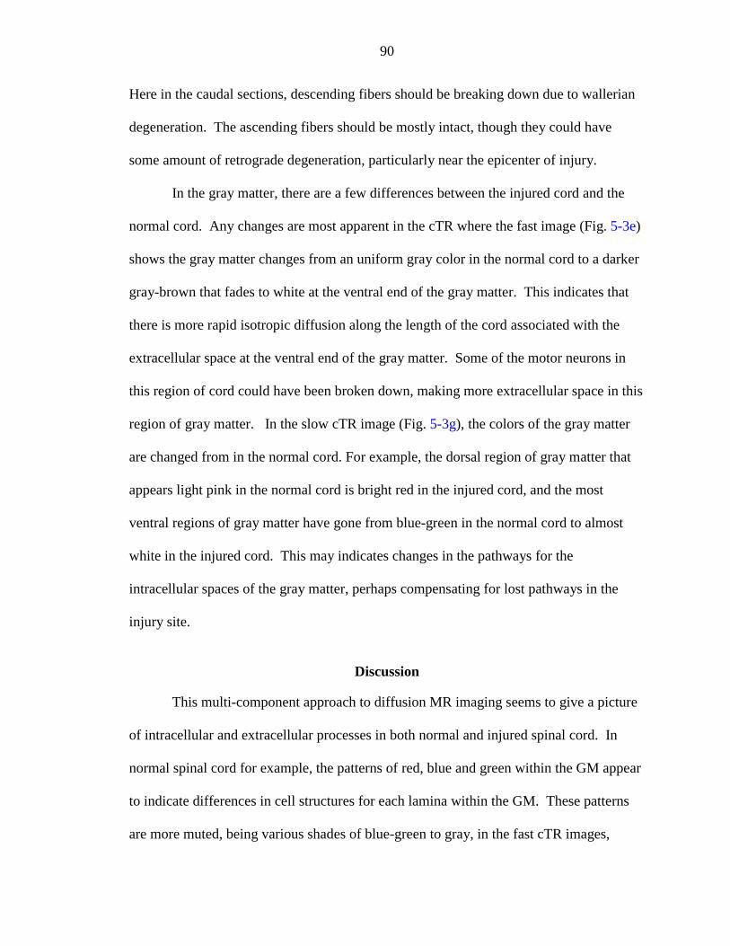
90
Here in the caudal sections, descending fibers should be breaking down due to wallerian
degeneration. The ascending fibers should be mostly intact, though they could have
some amount of retrograde degeneration, particularly near the epicenter of injury.
In the gray matter, there are a few differences between the injured cord and the
normal cord. Any changes are most apparent in the cTR where the fast image (Fig. 5-3e)
shows the gray matter changes from an uniform gray color in the normal cord to a darker
gray-brown that fades to white at the ventral end of the gray matter. This indicates that
there is more rapid isotropic diffusion along the length of the cord associated with the
extracellular space at the ventral end of the gray matter. Some of the motor neurons in
this region of cord could have been broken down, making more extracellular space in this
region of gray matter. In the slow cTR image (Fig. 5-3g), the colors of the gray matter
are changed from in the normal cord. For example, the dorsal region of gray matter that
appears light pink in the normal cord is bright red in the injured cord, and the most
ventral regions of gray matter have gone from blue-green in the normal cord to almost
white in the injured cord. This may indicates changes in the pathways for the
intracellular spaces of the gray matter, perhaps compensating for lost pathways in the
injury site.
Discussion
This multi-component approach to diffusion MR imaging seems to give a picture
of intracellular and extracellular processes in both normal and injured spinal cord. In
normal spinal cord for example, the patterns of red, blue and green within the GM appear
to indicate differences in cell structures for each lamina within the GM. These patterns
are more muted, being various shades of blue-green to gray, in the fast cTR images,
91
though they are brighter in the slow cTR images. This may be indicative of the
differences in the types of restriction seen by each diffusion component. The fast cTR
could indicate the fairly indistinguishable extracellular space, and the slow cTR could
indicate the various cell types and structures within the different laminae within the GM.
The uniform red of the WM clearly shows its long, thin tubelike structure. Also in the
normal spinal cord slow trace images (both cTR and gTR), the ring of white matter
immediately surrounding the gray matter (dark red in the cTR, and dark gray in the gTR)
appears to define the fasciculus proprius, a feature that does not appear in the fast
diffusion trace images.
In injury, this multi-compartmental approach to interpreting the apparent diffusion
tensor map is sensitive to changes occurring both rostral and caudal to the site of injury.
Though differences between normal and injured gray matter are seen, changes visualized
by this technique are most apparent in the white matter of the spinal cord. Degradation of
the axons and their accompanying myelin sheaths away from the cell body and/or injury
site as a result of injury to the axon or its cell body is called wallerian degeneration
(Becerra et al., 1995). By looking at the diffusion anisotropy it is possible to differentiate
normal nerves from demyelinated nerves (Ono et al., 1995). Ono et al. (1995) saw this
difference as a rise ADC of the in-plane diffusion coefficient and a fall in the ADC along
the length of the nerve, leading to a loss in anisotropy. By non-NMR methods, Sykova
(1997) saw that diffusion is more isotropic in the extracellular space of WM when axons
have incomplete myelination or are completely unmyelinated. In the fast component of
diffusion for the images presented here, there is a greater isotropy in the WM regions that
would be affected by demyelination due to wallerian degeneration. These same changes,
92
however, are not as apparent in the equivalent slow component graphs and images. The
exception to this observation is the dorsal funiculus, which would be the region of
greatest damage. Rostral to the site of injury, it stands out as damaged in every image
and graph. This diffusion technique seems particularly sensitive to Wallerian
degeneration that occurs as a result of trauma to the neural tissue. This is evidenced by
the darkening in the cTR of some white matter regions both rostral and caudal to the site
of injury.
The fast diffusion regime images appear to show changes from things like
demyelination of the axons, and cellular and axonal breakdown due to necrosis or
excitotoxic shock. Cellular matter that has been freed into the interstitial spaces
following the breakdown of cells and axons would slow the rate of diffusion through the
extracellular space, though a greater amount of space would be present due to loss of
cells. The slow diffusion regime images seem to show changes that would be apparent
from problems such as cellular edema indicated by a rise in the slow diffusion rate, or the
axon reaction (i.e. upregulation of neurofilaments and intracellular organelles as well as
chromatolysis) that would be indicated by a fall in the slow diffusion rate.
Further study is needed to better understand exactly what is being visualized by
the fast and slow diffusion compartments, though upon first inspection they seem to
demonstrate what is going on in the extracellular and intracellular spaces, respectively.
With a better understanding of the compartments being visualized, in vivo studies could
be performed with this technique. It would be useful to be able to follow a single animal
in a longitudinal study, visualizing the bulk cellular changes that are occurring

93
throughout the spinal cord as a result of trauma. With this multi-component diffusion
technique, such visualizations may ultimately be possible.
94
CHAPTER 6SUMMARY AND CONCLUSIONS
Medical science and research have become more advanced with the appearance of
new techniques, such as MRI, that allow pathologies to be visualized in living organisms.
With these new methods of looking at tissue in vivo comes the responsibility to
understand exactly what is being visualized with these methods before undertaking
treatment protocols. This responsibility includes clearly defining what patterns are
normal for the tissue being visualized within the chosen methodology. It also includes
understanding how various pathologies, including trauma and disease states, change the
patterns seen by the chosen technique. One method of demonstrating and defining
normal and pathological states is to take measurements of the tissue samples ex vivo.
Such measurements can be easily correlated with light microscopy done on histological
sections of the same or other tissue samples. The problem with such studies is that they
are static, yielding only a single time point for the sample in question. Tissue in vivo is
dynamic – interacting with its environment in ways that fixed, ex vivo samples cannot.
This is not to say that measurements made ex vivo cannot be useful. In fact,
making measurements on ex vivo samples can yield knowledge that is useful,
qualitatively, in defining what is seen in vivo. However, as seen in Chapter 2, the sample
preparation can make significant changes in measured MR parameters such as T2
relaxation rate and diffusion rate. In order to draw parallels between the in vivo and ex
vivo cases, a balance must be achieved between the need to have a sample that will
95
remain stable indefinitely and the desire to have a sample that closely resembles a
“snapshot” of the tissue in vivo. Tissue fixed with 4% formaldehyde solution appears to
most closely resembling tissue in vivo, though any fixative surrounding the tissue will
negatively effect the T2 relaxation rate. It is strongly suggested that tissue samples be
bathed in PBS prior to making MR imaging measurements in order to reduce the effect of
fixation on T2-relaxation. However, if the samples have been fixed with formaldehyde
alone it is suggested that the tissue sample be promptly returned to the fixative solution in
order to prevent tissue degradation.
In formaldehyde fixed human brain tissue, two T2 relaxation components were
seen, a long and a short relaxation time. The two components had widely disparate
relaxation rates, though these T2 relaxation components had volume ratios similar to the
extracellular and intracellular volume ratios. This led to the assumption that the long
relaxation time measured water is in the extracellular spaces and the short relaxation time
measured water is in the intracellular spaces. Two diffusion rate components were also
seen in these samples, a fast diffusing species and a slow diffusing species. Although the
two components had volume ratios that differed from the expected extracellular and
intracellular volume ratios, these volume ratios were relaxation-weighted. By using the
measured T2 relaxation rates and making the assumption that the water species with the
long relaxation rate was the same as the water species with the fast diffusion time, the
relaxation could be assumed to be uncoupled from the diffusion volume ratios. After
removing T2 relaxation, the diffusion measurement volume ratios closely matched the
volume ratios determined for the T2 relaxation rate, making the volume ratios closer to
those expected for the extracellular and intracellular spaces.
96
Although T2 relaxation seems to be the major contributor in changing the volume
ratios from the expected, other things could contribute, like exchange between water
compartments, differing proton densities in the two compartments, and differing
restrictions in each compartment. The exchange rate between these two spaces seems to
be long, as evidenced by the appearance of two distinct diffusion rates, allowing a
biexponential diffusion fit to the data. The dwell time in each space needs to be known in
order to understand how quantitatively these fast and slow diffusion components measure
the extracellular and intracellular diffusion rates. Eventually this exchange rate must be
quantified in order to know with certainty that the two diffusion components are
representative of the extracellular and intracellular spaces. One method of finding the
exchange rate would to take diffusion measurements at a variety of diffusion times (from
as short as possible to as long as possible), and fitting for the exchange parameter as well
as the diffusion rates.
However, since the two compartments have volume fractions resembling the
extracellular and intracellular space volume fractions, the assumption is made that the
two compartments are similar to, if not the same as, those spaces. By doing the imaging
experiment in rat spinal cord, further evidence was seen that the two diffusion
components may represent the extracellular and intracellular spaces. The volume
fractions seen in GM and WM regions of the cord (Figure 4-1) were approximately equal
to those found in the brain tissue before removal of the T2 relaxation rates. This implies
that the two components being imaged are the same components as were found in the
spectroscopy on the brain tissue.
97
The fast and slow grayscale trace images (Figures 4-4a and 4-4b) had appearances
very different from one another. Those differences seem to be due to the similar nature
of extracellular space in each tissue type, and the dissimilar nature of intracellular space
in different tissue types. In the slow component images there is a dark ring around the
gray matter that coincides with the propriospinal system (c and d in Figures 5-1, 5-2 and
5-3; b and d in Figures 5-4, 5-5 and 5-6). This ring is not visible in any of the fast
component images. This region is white matter consisting of short, thin axons that
ascend and descend short distances between segments. This piece of evidence seems to
indicate that the extracellular spaces (fast component) in this region appear no different
that any other white matter region, but the intracellular spaces (slow component) are
shorter and more restricted than other white matter regions. In the fast component, the
gray matter appears more isotropic, while in the slow component the various laminae
show up in varying colors of red, green and blue. This is yet another piece of data that
suggests the fast and slow components are indicative of the extracellular and intracellular
compartments within the tissue.
In injury, diffusion tensor imaging can show the amount of white matter spared at
the injury site. Also, it seems particularly sensitive to wallerian degeneration in white
matter away from the site of injury. This was seen most clearly in the color trace images
rostral and caudal to the site of injury (e and g in Figues 5-1 and 5-3). The changes
apparent in the fast diffusion component appear consistent with demyelinaton of the
axons, and cellular and axonal breakdown due to necrosis or excitotoxic shock. The
changes apparent in the slow diffusion regime appear consistent with cellular edema or
the axon reaction. In other words, the fast diffusion component seems to show the
98
changes that occur in the extracellular space and the slow diffusion component seems to
show changes that occur in the intracellular space. More measurements must be taken in
order to sort out if the two components are truly representative of the extracellular and
intracellular spaces, but many of the details seen in these studies seem to indicate that this
assumption is correct.
From this work, there are two take-home messages for the general MR
community. First, when doing ex vivo work, be aware that tissue preparation can have a
large effect on the measurement made. Second, when doing monoexponential diffusion
measurements (both ADC and ADT), the diffusion time, echo time, and maximum b
value should be equivalent for all experiments being compared. Using a different
diffusion time, even if the b values are the same will lead to different quantitative
answers as can be seen in q-space studies (Meier et al., 1999). In nervous tissue, there
are at least two different diffusion compartments that seem to have very disparate T2
relaxation rates. Utilizing a different echo time will lead to each component contributing
a different volume fraction. By using different maximum b values, different fractions of
each compartment contribute to the monoexponential fit as demonstrated by the
differences in the dashed and dot-dashed lines in Figures 3-1 and 3-2.
Lately, in clinical work, there has been a drive towards taking data at higher and
higher b values. A linear fit to data taken in this manner may in no way be a quantitative
measure of the diffusion rate. Instead a non-linear fit to the data should be performed,
and that is difficult without doing 5 points per direction or more and taking the b values
up to at least 6000 s/mm2. It must be kept in mind that a linear fit to data taken up to a b
value of 1000 s/mm2 will not be completely quantitative, but it can give an average
99
qualitative picture of the diffusion. Also, by keeping TE long it may be possible to focus
more clearly on the fast diffusion regime, even at low b values, at the expense of having
exchange take a larger role in the observed problems and losing the slow diffusion
information. If TE is kept short, big gradients will allow both δ and ∆ to be shorter, thus
limiting the problems caused by T2 relaxation and exchange. Also, with shorter δ, the
short time approximation (δ << ∆) is more valid (Helmer et al., 1995). In order to better
understand the various mechanisms that alter the diffusion rates and observed volume
fractions we are planning studies of the T2 relaxation rate, diffusion rates at multiple
diffusion times, and diffusion at various values of TE.
100
GLOSSARY
anisotropic : exhibiting the property of having different values when measured along axesin different directions
anterior : the front surface of the human body; equivalent to ventral in animal anatomy
apoptosis : cell death where the cell encapsulates and is removed
axon reaction : a combination of chromatolysis and the upregulation of neurofilamentsand intracellular organelles that occurs due to axonal injury; an axon in this statelies somewhere between apoptosis and necrosis
chromatolysis : the dissolution and breaking up of intracellular organelles
correlation time : the order of time it takes a molecule to turn through 1 radian, or thetime for a molecule to move through a distance comparable to it’s dimensions
corticospinal tract : white matter region of descending axons going from the cortex downthe spine; located in the dorsal section of the spinal cord, ventral to the fasciculusgracilis
diffusion : the process where particles (solid, liquid and/or gas) intermingle as the resultof spontaneous random motion caused by thermal agitation
dipole : a pair of equal and opposite electric or magnetic charges separated by a smalldistance
dorsal : the back or upper surface in an animal; equivalent to posterior in humans
dorsal spinocerebellar tract : white matter region of ascending axons going from the spineto the cerebellum; located in the dorsolateral section of the white matter
dorsolateral : on the side towards the back surface of an animal
exsanguinate : to drain the blood out of
extracellular : outside the cell; the region between the cells making up the interstitialmatrix of the tissue
101
ex vivo : out of life, or in non-living tissue
fasciculus gracilis (Gracile Fasciculus) : white matter region of ascending axons in thedorsal region of the spine, between the dorsal columns of gray matter
fasciculus proprius (propriospinal tract) : white matter region of short ascending anddescending axons that move between spinal segments; located just dorsal and justventral to the gray matter
fix : to kill, harden, and preserve tissue for later study
fixative : a substance used to fix living tissue for later study
formaldehyde : a molecule with the chemical formula CH2O that can be used as a tissuefixative
gluteraldehyde : a molecule with the chemical formula OCH(CH2)3CHO that can be usedas a tissue fixative
histology : branch of anatomy that deals with tissue structure as can be visualized by amicroscope
intracellular : inside the cell
isotropic : exhibiting the property of having the same value when measured along axes indifferent directions
in vivo : in the living tissue or animal
in vitro : in an artificial environment outside the living animal
Karnowsky’s solution : a fixative solution that is a mixture of 5% gluteraldehyde and 4%formaldehyde
lamina : regions of different cell structure within the gray matter; they are labelled withRoman numeral I to X on the figure in Appendix B.
Larmor frequency : the precessional frequency of a nucleus in a magnetic field given bythe equation ω0 = γ B0 where γ is the gyromagnetic ratio for the nucleus and B0 isthe strength of the magnetic field
lateral : on the side
lateral spinothalamic tract : white matter region of ascending axons going from the spineup to the thalamus; located in the lateral portion of the spine
102
lateral vestibulospinal tract : white matter region of descending axons going from thebrain down the spine; located in the ventrolateral portion of the cord
necrosis : localized death of living tissue
perfuse : force fluid through the body by way of the blood vessels
permeable : having pores or openings that allow the passage of liquids or gasses
porous media : solid substance that has pores making it permeable to liquid
posterior : the back surface of the human body; equivalent to dorsal in animal anatomy
propriospinal tract : see fasciculus proprius
pyramidal tract (Tractus Pyramidalis) : see corticospinal tract
quadrupole : a system consisting of two dipoles with equal and opposite magneticmoments
rubrospinal tract : white matter region of axons descending from the red nucleus in thebrain down the spine; located in the dorsolateral region of the spine
semipermeable : partially, but not wholly and freely, permeable
spino-olivary tract : white matter region of axons ascending from the spine to the brain;located in the ventrolateral region of the spine
spinotectal tract : white matter region of axons ascending from the spine to the brain;located in the ventrolateral region of the spine, just interior to the spino-olivarytract of the spine
T1 Relaxation : also known as spin-lattice, or longitudinal relaxation; characterized by thereturn of the net magnetization to the ground state (i.e. the state where the netmagnetization is along the main magnetic field) from the high-energy stateinduced by an RF pulse
T2 Relaxation : also known as spin-spin, or transverse relaxation; characterized byadjacent spins in high and low energy states exchanging energy without losingthat energy to the surrounding lattice
tensor : a generalized vector with more than three components each of which is a functionof the coordinates of an arbitrary point in space of an appropriate number ofdimensions
103
tortuosity : the quality of a substance as being tortuous (i.e. marked by repeated twists,bends, or turns)
ventral : the front or lower surface in an animal; equivalent to anterior in humans
ventral spinocerebellar tract : white matter region of axons ascending from the spine up tothe cerebellum; located in the ventral region of the spine
ventral spinothalamic tract : white matter region of axons ascending from the spine up tothe thalamus; located in the ventral region of the spine
ventrolateral : on the side towards the front surface of an animal
wallerian degeneration : degradation of the axons and their accompanying myelin sheathsaway from the cell body and/or injury site as a result of injury to the axon or itscell body
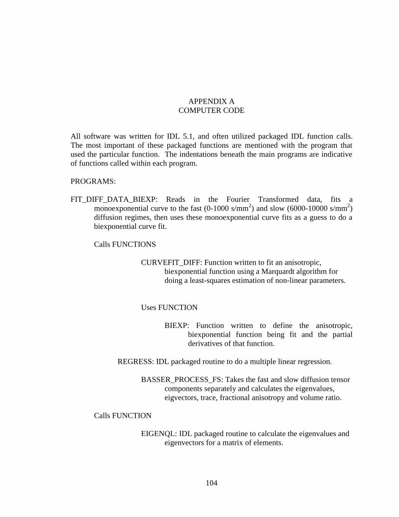
104
APPENDIX ACOMPUTER CODE
All software was written for IDL 5.1, and often utilized packaged IDL function calls.The most important of these packaged functions are mentioned with the program thatused the particular function. The indentations beneath the main programs are indicativeof functions called within each program.
PROGRAMS:
FIT_DIFF_DATA_BIEXP: Reads in the Fourier Transformed data, fits amonoexponential curve to the fast (0-1000 s/mm2) and slow (6000-10000 s/mm2)diffusion regimes, then uses these monoexponential curve fits as a guess to do abiexponential curve fit.
Calls FUNCTIONS
CURVEFIT_DIFF: Function written to fit an anisotropic,biexponential function using a Marquardt algorithm fordoing a least-squares estimation of non-linear parameters.
Uses FUNCTION
BIEXP: Function written to define the anisotropic,biexponential function being fit and the partialderivatives of that function.
REGRESS: IDL packaged routine to do a multiple linear regression.
BASSER_PROCESS_FS: Takes the fast and slow diffusion tensorcomponents separately and calculates the eigenvalues,eigvectors, trace, fractional anisotropy and volume ratio.
Calls FUNCTION
EIGENQL: IDL packaged routine to calculate the eigenvalues andeigenvectors for a matrix of elements.
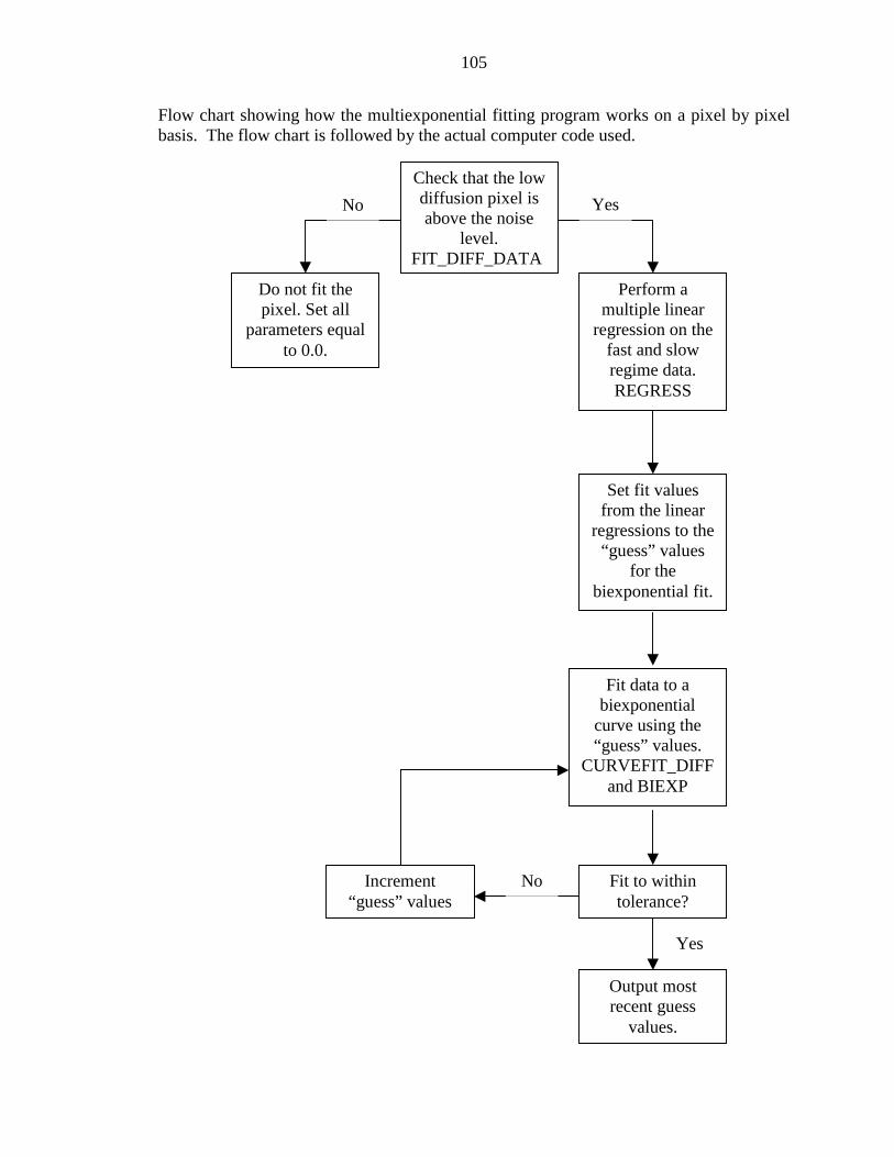
105
Flow chart showing how the multiexponential fitting program works on a pixel by pixelbasis. The flow chart is followed by the actual computer code used.
Check that the lowdiffusion pixel isabove the noise
level.FIT_DIFF_DATA
YesNo
Do not fit thepixel. Set all
parameters equalto 0.0.
Perform amultiple linear
regression on thefast and slowregime data.REGRESS
Set fit valuesfrom the linear
regressions to the“guess” values
for thebiexponential fit.
Fit data to abiexponential
curve using the“guess” values.
CURVEFIT_DIFFand BIEXP
Fit to withintolerance?
Output mostrecent guess
values.
Yes
NoIncrement“guess” values

106
The program FIT_DIFF_DATA_BIEXP.pro takes the data that has been FourierTransformed and fits it to several curves: two monoexponential curves (using thefunction REGRESS) and one biexponential curve (using the functions CURVEFIT_DIFFand BIEXP).
;**** Begin Main Program *****; This program takes ft data and fits it to monoexponential and biexponential curves; NAME:; FIT_DIFF_DATA_BIEXP;; PURPOSE:; Fits diffusion data to a biexponential curve; Uses the functions CURVEFIT_DIFF and BIEXP;; CATEGORY:; Curvefit;; CALLING SEQUENCE:; .RUN FIT_DIFF_DATA_BIEXP;; INPUTS:;; KEYWORDS:; NONE;; OUTPUTS:; alpha_fast : the fast diffusion values; alpha_slow : the slow diffusion values; alpha : the S0f, S0s, fast and slow diffusion values; sigma : error matrix for the biexponential tensor fit;; OPTIONAL OUTPUT PARAMETERS:; NONE;; COMMON BLOCKS:; NONE.;; SIDE EFFECTS:; NONE.;; RESTRICTIONS:; NONE.;; PROCEDURE:;
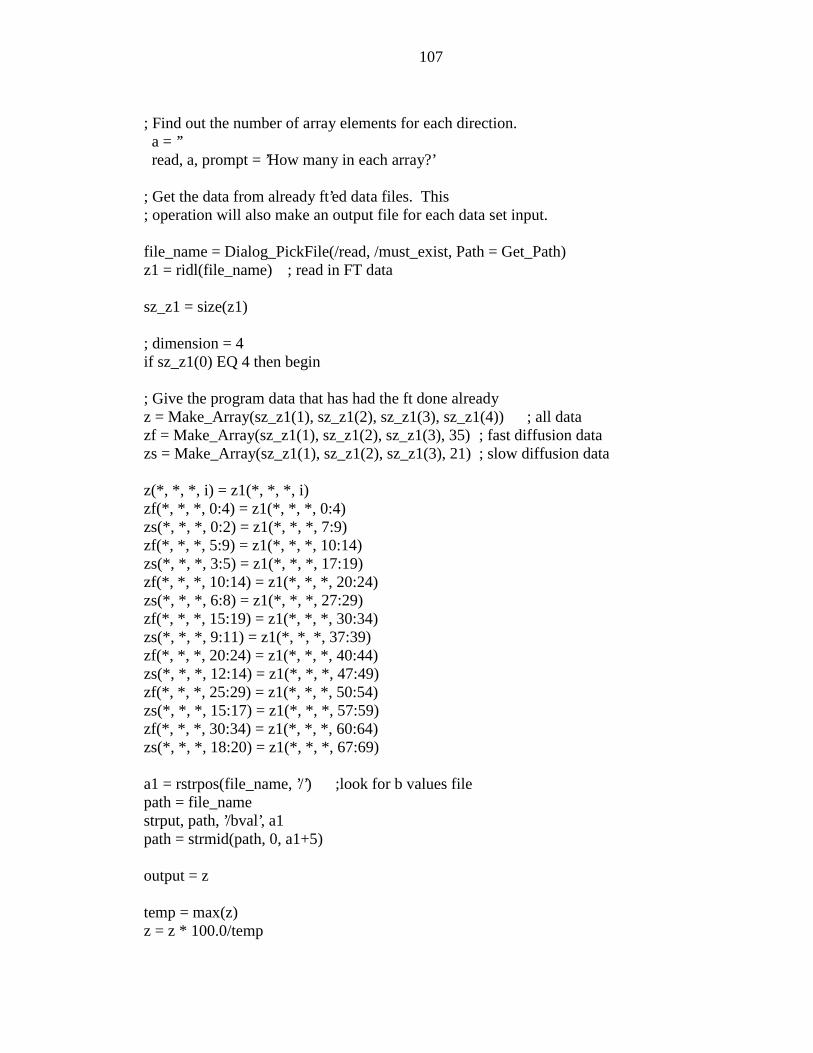
107
; Find out the number of array elements for each direction. a = ’’ read, a, prompt = ’How many in each array?’
; Get the data from already ft’ed data files. This; operation will also make an output file for each data set input.
file_name = Dialog_PickFile(/read, /must_exist, Path = Get_Path)z1 = ridl(file_name) ; read in FT data
sz_z1 = size(z1)
; dimension = 4if sz_z1(0) EQ 4 then begin
; Give the program data that has had the ft done alreadyz = Make_Array(sz_z1(1), sz_z1(2), sz_z1(3), sz_z1(4)) ; all datazf = Make_Array(sz_z1(1), sz_z1(2), sz_z1(3), 35) ; fast diffusion datazs = Make_Array(sz_z1(1), sz_z1(2), sz_z1(3), 21) ; slow diffusion data
z(*, *, *, i) = z1(*, *, *, i)zf(*, *, *, 0:4) = z1(*, *, *, 0:4)zs(*, *, *, 0:2) = z1(*, *, *, 7:9)zf(*, *, *, 5:9) = z1(*, *, *, 10:14)zs(*, *, *, 3:5) = z1(*, *, *, 17:19)zf(*, *, *, 10:14) = z1(*, *, *, 20:24)zs(*, *, *, 6:8) = z1(*, *, *, 27:29)zf(*, *, *, 15:19) = z1(*, *, *, 30:34)zs(*, *, *, 9:11) = z1(*, *, *, 37:39)zf(*, *, *, 20:24) = z1(*, *, *, 40:44)zs(*, *, *, 12:14) = z1(*, *, *, 47:49)zf(*, *, *, 25:29) = z1(*, *, *, 50:54)zs(*, *, *, 15:17) = z1(*, *, *, 57:59)zf(*, *, *, 30:34) = z1(*, *, *, 60:64)zs(*, *, *, 18:20) = z1(*, *, *, 67:69)
a1 = rstrpos(file_name, ’/’) ;look for b values filepath = file_namestrput, path, ’/bval’, a1path = strmid(path, 0, a1+5)
output = z
temp = max(z)z = z * 100.0/temp
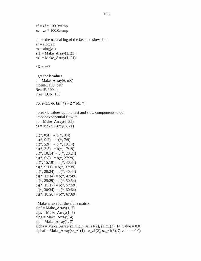
108
zf = zf * 100.0/tempzs = zs * 100.0/temp
; take the natural log of the fast and slow datazf = alog(zf)zs = alog(zs)zf1 = Make_Array(1, 21)zs1 = Make_Array(1, 21)
nX = a*7
; get the b valuesb = Make_Array(6, nX)OpenR, 100, pathReadF, 100, bFree_LUN, 100
For i=3,5 do b(i, *) = 2 * b(i, *)
; break b values up into fast and slow components to do; monoexponential fit withbf = Make_Array(6, 35)bs = Make_Array(6, 21)
bf(*, 0:4) = b(*, 0:4)bs(*, 0:2) = b(*, 7:9)bf(*, 5:9) = b(*, 10:14)bs(*, 3:5) = b(*, 17:19)bf(*, 10:14) = b(*, 20:24)bs(*, 6:8) = b(*, 27:29)bf(*, 15:19) = b(*, 30:34)bs(*, 9:11) = b(*, 37:39)bf(*, 20:24) = b(*, 40:44)bs(*, 12:14) = b(*, 47:49)bf(*, 25:29) = b(*, 50:54)bs(*, 15:17) = b(*, 57:59)bf(*, 30:34) = b(*, 60:64)bs(*, 18:20) = b(*, 67:69)
; Make arrays for the alpha matrixalpf = Make_Array(1, 7)alps = Make_Array(1, 7)alpg = Make_Array(14)alp = Make_Array(1, 7)alpha = Make_Array(sz_z1(1), sz_z1(2), sz_z1(3), 14, value = 0.0)alphaf = Make_Array(sz_z1(1), sz_z1(2), sz_z1(3), 7, value = 0.0)
109
alphas = Make_Array(sz_z1(1), sz_z1(2), sz_z1(3), 7, value = 0.0)sig = Make_Array(sz_z1(1), sz_z1(2), sz_z1(3), 14, value = 0.0)
; weightswtf = replicate(1.0, 35)wts = replicate(1.0, 21)weights = replicate(1.0, a*7)z1 = z(*,*,*,0)z1 = reform(z1, sz_z1(1), sz_z1(2), sz_z1(3))
For i = 0, sz_z1(1)-1 Do Begin For j = 0, sz_z1(2)-1 Do Begin For k = 0, sz_z1(3)-1 Do Begin If z1(i, j, k) GT 2.0 Then Begin zf1 = zf(i, j, k, *) zf1 = reform(zf1, 35) zs1 = zs(i, j, k, *) zs1 = reform(zs1, 21)
alpf = Regress(-bf, zf1, wtf, yfitf, a0f)alps = Regress(-bs, zs1, wts, yfits, a0s)If z1(i, j, k) GE 30.0 Then alps = alps*0.0alphaf(i, j, k, 0) = exp(a0f) - exp(a0s)alphaf(i, j, k, 1:6) = alpfalphas(i, j, k, 0) = exp(a0s)alphas(i, j, k, 1:6) = alpsalpf(1:3) = alpf(1:3)*2.5alpg(0:6) = alphaf(i, j, k, *)alpg(7:13) = alphas(i, j, k, *)z2 = z(i, j, k, *)z2 = reform(z2,70)If z1(i,j,k) LT 30.0 then yfit = curvefit_diff(b, z2, weights, $
alpg, sigma, Function_Name = ’biexp’, iter = iter, $chisq = chisq)
print, iteralpha(i, j, k, *) = alpgsig(i, j, k, *) = sigma
EndIfprint, i, j, k
EndFor EndForEndForendif
alpha = abs(alpha)df = alpha(*,*,*,1:6)ds = alpha(*,*,*,8:13)
110
df = df*1000000ds = ds*1000000z0f = alpha(*,*,*,0)z0s = alpha(*,*,*,7)z0f = z0f*100z0s = z0s*100zfs = z0f + z0sa = where(df gt 3000)df(a) = 3000a = where(ds gt 800)ds(a) = 800df = round(df)df = fix(df)ds = round(ds)ds = fix(ds)z0f = round(z0f)z0f = fix(z0f)z0s = round(z0s)z0s = fix(z0s)zfs = round(zfs)zfs = fix(zfs)
sz1 = size(alphaf)OpenW, 100, ’alpha_fast.flt’WriteU, 100, sz1, alphafFree_LUN, 100
alphaf(*,*,*,0) = alphaf(*,*,*,0)*1000alphaf(*,*,*,1:5) = alphaf(*,*,*,1:5)*1000000alphaf = fix(alphaf)
OpenW, 100, ’alpha_fast.im’WriteU, 100, alphafFree_LUN, 100
OpenW, 100, ’alpha_slow.flt’WriteU, 100, sz1, alphasFree_LUN, 100
alphas(*,*,*,0) = alphas(*,*,*,0)*1000alphas(*,*,*,1:5) = alphas(*,*,*,1:5)*1000000alphas = fix(alphas)
OpenW, 100, ’alpha_slow.im’WriteU, 100, alphasFree_LUN, 100
111
sz = size(alpha)OpenW, 100, ’alpha.flt’WriteU, 100, sz, alphaFree_LUN, 100
OpenW, 100, ’sigma.flt’WriteU, 100, sz, sigmaFree_LUN, 100
End
The procedure curvefit_diff is modified from the curvefit routine written by IDL. Thisfunction is modified to fit a biexponential curve, specifically and utilizes the functionbiexp to define the curve and its partial derivatives.
FUNCTION CURVEFIT_DIFF, x, y, weights, a, $sigma, FUNCTION_NAME = Function_Name, $
ITMAX=itmax, ITER=iter, TOL=tol, CHI2=chi2, $ NODERIVATIVE=noderivative, CHISQ=chisq; NAME:; CURVEFIT_DIFF;; PURPOSE:; Non-linear least squares fit to a function of an arbitrary; number of parameters. Funtion used will be a biexponential; function. This function will have 14 unknowns to calculate; from the guess and the partial derivatives.;;; CATEGORY:; Curve and Surface Fitting.;; CALLING SEQUENCE:; Result = CURVEFIT_DIFF(X1, X2, X3, X4, X5, X6, Y, Weights, $; A, SIGMA, FUNCTION_NAME = name, $; ITMAX=ITMAX, ITER=ITER, TOL=TOL, /NODERIVATIVE);; INPUTS:; Xi: A row vector of independent variables. This routine does; not manipulate or use values in X, it simply passes X; to the user-written function. These are the vectors of; b values. (i = 1, 2, 3, 4, 5, 6);; Y: A row vector containing the dependent variable.
112
;; Weights: A row vector of weights, the same length as Y.; For no weighting,; Weights(i) = 1.0.; For instrumental (Gaussian) weighting,; Weights(i)=1.0/sigma(i)^2; For statistical (Poisson) weighting,; Weights(i) = 1.0/y(i), etc.;; A: A vector, with as many elements as the number of terms, that; contains the initial estimate for each parameter. IF A is double-; precision, calculations are performed in double precision,; otherwise they are performed in single precision. Fitted parameters; are returned in A.;; KEYWORDS:; FUNCTION_NAME: The name of the function (actually, a procedure) to; fit. IF omitted, "FUNCT" is used. The procedure must be written as; described under RESTRICTIONS, below. This program utilizes the function; BIEXP;; ITMAX: Maximum number of iterations. Default = 100.; ITER: The actual number of iterations that were performed; TOL: The convergence tolerance. The routine returns when the; relative decrease in chi-squared is less than TOL in an; iteration. Default = 1.e-7.; CHISQ: The value of reduced chi-squared on exit; NODERIVATIVE: IF this keyword is set THEN the user procedure will not; be requested to provide partial derivatives. The partial; derivatives will be estimated in CURVEFIT using forward; differences. IF analytical derivatives are available they; should always be used.;; OUTPUTS:; Returns a vector of calculated values.; A: A vector of parameters containing fit.;; OPTIONAL OUTPUT PARAMETERS:; Sigma: A vector of standard deviations for the parameters in A.;; COMMON BLOCKS:; NONE.;; SIDE EFFECTS:; NONE.;
113
; RESTRICTIONS:; The function to be fit must be defined and called BIEXP,; FUNCT, Xi, A, F, PDER; where:; Xi= Variables passed into CURVEFIT. It is the job of the user-written; function to interpret this variable.; A = Vector of NTERMS function parameters, input.; F = Vector of NPOINT values of function, y(i) = funct(x), output.; PDER = Array, (NPOINT, NTERMS), of partial derivatives of funct.; PDER(I,J) = DErivative of function at ith point with; respect to jth parameter. Optional output parameter.; PDER should not be calculated IF the parameter is not; supplied in call. IF the /NODERIVATIVE keyword is set in the; call to CURVEFIT THEN the user routine will never need to; calculate PDER.;; PROCEDURE:; Modified from "CURFIT", least squares fit to a non-linear; function, pages 237-239, Bevington, Data Reduction and Error; Analysis for the Physical Sciences. This is adapted from:; Marquardt, "An Algorithm for Least-Squares Estimation of Nonlinear; Parameters", J. Soc. Ind. Appl. Math., Vol 11, no. 2, pp. 431-441,; June, 1963.;; Iterations are performed until the chi square changes by; only TOL or until ITMAX iterations have been performed.;; The initial guess of the parameter values should be; as close to the actual values as possible or the solution; may not converge.;
ON_ERROR,2 ;Return to caller IF error
x1 = x(0, *)x2 = x(1, *)x3 = x(2, *)x4 = x(3, *)x5 = x(4, *)x6 = x(5, *)
;Name of function to fit
IF n_elements(function_name) LE 0 THEN function_name = "FUNCT"
IF n_elements(tol) EQ 0 THEN tol = 1.e-5 ;Convergence tolerance
114
IF n_elements(itmax) EQ 0 THEN itmax = 500 ;Maximum # iterations type = size(a) type = type[type[0]+1] double = type EQ 5
IF (type ne 4) AND (type ne 5) THEN a = float(a) ;Make params floating
; IF we will be estimating partial derivatives THEN compute machine ; precision
IF keyword_set(NODERIVATIVE) THEN BEGIN res = machar(DOUBLE=double) eps = sqrt(res.eps) ENDIF
nterms = n_elements(a) ; # of parameters nfree = n_elements(y) - nterms ; Degrees of freedom
IF nfree LE 0 THEN message, ’Curvefit - not enough data points.’
flambda = 0.001 ;Initial lambda diag = lindgen(nterms)*(nterms+1) ; Subscripts of diagonal elements
; Define the partial derivative array
IF double THEN pder = dblarr(n_elements(y), nterms) $ ELSE pder = fltarr(n_elements(y), nterms); FOR iter = 1, itmax DO BEGIN ; Iteration loop
; Evaluate alpha and beta matricies.
IF keyword_set(NODERIVATIVE) THEN BEGIN
; Evaluate function and estimate partial derivatives CALL_PROCEDURE, Function_name, x1, x2, x3, x4, x5, x6, $
a, yfit
FOR term=0, nterms-1 DO BEGIN
p = a ; Copy current parameters
; Increment size for forward difference derivative inc = eps * abs(p[term]) IF (inc EQ 0.) THEN inc = eps p[term] = p[term] + inc
115
CALL_PROCEDURE, function_name, x1, x2, x3, x4, x5, x6, $ p, yfit1
pder[0,term] = (yfit1-yfit)/inc
ENDFOR ENDIF ELSE BEGIN
; The user’s procedure will return partial derivatives call_procedure, function_name, x1, x2, x3, x4, x5, x6, $
a, yfit, pder
ENDELSE
IF nterms EQ 1 THEN pder = reform(pder, n_elements(y), 1)
beta = (y-yfit)*Weights # pder alpha = transpose(pder) # (Weights # (fltarr(nterms)+1)*pder)
; save current values of return parameters
sigma1 = sqrt( 1.0 / alpha[diag] ) ; Current sigma. sigma = sigma1
chisq1 = total(Weights*(y-yfit)^2)/nfree ; Current chi squared. chisq = chisq1
yfit1 = yfit
done_early = chisq1 LT total(abs(y))/1e7/NFREE IF done_early THEN GOTO, done
c = sqrt(alpha[diag]) c = c # c
lambdaCount = 0
REPEAT BEGIN
lambdaCount = lambdaCount + 1
; Normalize alpha to have unit diagonal.
array = alpha / c
; Augment the diagonal.
116
array[diag] = array[diag]*(1.+flambda)
; Invert modified curvature matrix to find new parameters.
IF n_elements(array) EQ 1 THEN array = (1.0 / array) $ ELSE array = invert(array)
b = a + array/c # transpose(beta) ; New params
call_procedure, function_name, x1, x2, x3, x4, x5, x6, $ b, yfit ; Evaluate function
chisq = total(Weights*(y-yfit)^2)/nfree ; New chisq sigma = sqrt(array[diag]/alpha[diag]) ; New sigma
IF (finite(chisq) EQ 0) OR $ (lambdaCount GT 30 AND chisq GE chisq1) THEN BEGIN
; Reject changes made this iteration, use old values.
yfit = yfit1 sigma = sigma1 chisq = chisq1
message, ’Failed to converge’, /INFORMATIONAL
GOTO, done
ENDIF
flambda = flambda*10. ; Assume fit got worse
ENDREP UNTIL chisq LE chisq1
flambda = flambda/100.
a=b ; Save new parameter estimate.
IF ((chisq1-chisq)/chisq1) LE tol THEN GOTO,done ;Finished? ENDFOR ;iteration loop; MESSAGE, ’Failed to converge’, /INFORMATIONAL
a = findgen(nterms)*0.0;done: chi2 = chisq ; Return chi-squared (chi2 obsolete-still works) IF done_early THEN iter = iter - 1 return,yfit ; return result
117
END
;**** begin biexp procedure *****; This procedure gives the biexponential equation being fit; and the partial derivatives for that equation; begin fit.
PRO biexp, x1, x2, x3, x4, x5, x6, a, f, pder; NAME:; BIEXP;; PURPOSE:; Give the biexponential function and its partial derivatives.; Used by the FUNCTION CURVEFIT_DIFF;; CATEGORY:; Function and partial derivatives;; CALLING SEQUENCE:; RESULT = CURVEFIT_DIFF(X1, X2, X3, X4, X5, X6, Y, Weights, $; A, SIGMA, FUNCTION_NAME = BIEXP, ITMAX = ITMAX, $
ITER = ITER, TOL = TOL, /NODERIVATIVE);; INPUTS:; Xi : a row vector of independent variables; A : a “guess” for the parameters being fit;; KEYWORDS:; NONE;; OUTPUTS:; F : the Function being fit; pder : the partial derivatives of the function being fit;; OPTIONAL OUTPUT PARAMETERS:; NONE;; COMMON BLOCKS:; NONE.;; SIDE EFFECTS:; NONE.;
118
; RESTRICTIONS:; Must be called with the CURVEFIT_DIFF function;; PROCEDURE:;bf1x = exp(-a(1)*x1)bf2x = exp(-a(2)*x2)bf3x = exp(-a(3)*x3)bf4x = exp(-a(4)*x4)bf5x = exp(-a(5)*x5)bf6x = exp(-a(6)*x6)
bs1x = exp(-a(8)*x1)bs2x = exp(-a(9)*x2)bs3x = exp(-a(10)*x3)bs4x = exp(-a(11)*x4)bs5x = exp(-a(12)*x5)bs6x = exp(-a(13)*x6)
f = a(0)*bf1x*bf2x*bf3x*bf4x*bf5x*bf6x + a(7)*bs1x*bs2x*bs3x*bs4x*bs5x*bs6x
IF N_PARAMS() GE 9 THEN BEGIN pder=Fltarr(N_Elements(x1), 14) pder(*, 0) = bf1x*bf2x*bf3x*bf4x*bf5x*bf6x pder(*, 1) = -a(0)*x1*bf1x*bf2x*bf3x*bf4x*bf5x*bf6x pder(*, 2) = -a(0)*x2*bf1x*bf2x*bf3x*bf4x*bf5x*bf6x pder(*, 3) = -a(0)*x3*bf1x*bf2x*bf3x*bf4x*bf5x*bf6x pder(*, 4) = -a(0)*x4*bf1x*bf2x*bf3x*bf4x*bf5x*bf6x pder(*, 5) = -a(0)*x5*bf1x*bf2x*bf3x*bf4x*bf5x*bf6x pder(*, 6) = -a(0)*x6*bf1x*bf2x*bf3x*bf4x*bf5x*bf6x
pder(*, 7) = bs1x*bs2x*bs3x*bs4x*bs5x*bs6x pder(*, 8) = -a(7)*x1*bs1x*bs2x*bs3x*bs4x*bs5x*bs6x pder(*, 9) = -a(7)*x2*bs1x*bs2x*bs3x*bs4x*bs5x*bs6x pder(*, 10) = -a(7)*x3*bs1x*bs2x*bs3x*bs4x*bs5x*bs6x pder(*, 11) = -a(7)*x4*bs1x*bs2x*bs3x*bs4x*bs5x*bs6x pder(*, 12) = -a(7)*x5*bs1x*bs2x*bs3x*bs4x*bs5x*bs6x pder(*, 13) = -a(7)*x6*bs1x*bs2x*bs3x*bs4x*bs5x*bs6xENDIF
END
;**** End biexp procedure *****

119
The program basser_process_fs takes the fast and slow diffusion tensor elements andcalculates the eigenvalues, eigenvectors, trace, fractional anisotropy and volume ratio foreach voxel.
; Begin program basser_process_fs; NAME:; BASSER_PROCESS_FS;; PURPOSE:; Calculates the eigenvalues, eigenvectors and trace; for each voxel in the diffusion tensor; both the fast and the slow; tensor elements get their own set of calculations;; CATEGORY:; Calculation of parameters by Basser (1995);; CALLING SEQUENCE:; .RUN BASSER_PROCESS_FS;; INPUTS:;; KEYWORDS:; NONE;; OUTPUTS:; Fast and slow eigenvalues, eigenvectors, traces,; fractional anisotropy images and volume ratios;; OPTIONAL OUTPUT PARAMETERS:; NONE;; COMMON BLOCKS:; NONE.;; SIDE EFFECTS:; NONE.;; RESTRICTIONS:; NONE.;; PROCEDURE:;; Right now, calculates the eigenvalues, eigenvectors and trace; for each voxel in the diffusion tensor; both the fast and the slow; tensor elements get their own set of calculations
120
file_name = PickFile(/read, /must_exist, Path = Get_Path)
alpha = ridl(file_name)
sz_alpha = size(alpha)
alpha = abs(alpha)
xdim = sz_alpha(1)ydim = sz_alpha(2)zdim = sz_alpha(3)
Af_matrix = Make_array(3, 3)As_matrix = Make_array(3, 3)evalsf = Make_array(xdim, ydim, zdim, 3)evalss = Make_array(xdim, ydim, zdim, 3)evecsf = Make_array(xdim, ydim, zdim, 3, 3)evecss = Make_array(xdim, ydim, zdim, 3, 3)Trace_Df = Make_array(xdim, ydim, zdim)Trace_Ds = Make_array(xdim, ydim, zdim)detf = Make_array(xdim, ydim, zdim)dets = Make_array(xdim, ydim, zdim)
For x = 0, xdim-1 Do Begin For y = 0, ydim-1 Do Begin For z = 0, zdim-1 Do Begin Af_matrix = [[alpha(x, y, z, 1), alpha(x, y, z, 4), alpha(x, y, z, 5)], $
[alpha(x, y, z, 4), alpha(x, y, z, 2), alpha(x, y, z, 6)], $[alpha(x, y, z, 5), alpha(x, y, z, 6), alpha(x, y, z, 3)]]
eigenval = EIGENQL(Af_matrix, EIGENVECTORS = ev) evalsf(x, y, z, *) = eigenval evecsf(x, y, z, *, *) = ev Trace_Df(x, y, z) = TRACE(Af_matrix)/3 As_matrix = [[alpha(x, y, z, 8), alpha(x, y, z, 11), alpha(x, y, z, 12)], $
[alpha(x, y, z, 11), alpha(x, y, z, 9), alpha(x, y, z, 13)], $[alpha(x, y, z, 12), alpha(x, y, z, 13), alpha(x, y, z, 10)]]
eigenval = EIGENQL(As_matrix, EIGENVECTORS = ev) evalss(x, y, z, *) = eigenval evecsf(x, y, z, *, *) = ev Trace_Ds(x, y, z) = Trace(As_matrix)/3
121
EndFor EndForEndFor
Deviatoricf = sqrt(((evalsf(*,*,*,0) - Trace_Df)^2 + $ (evalsf(*,*,*,1) - Trace_Df)^2 + $ (evalsf(*,*,*,2) - Trace_Df)^2))
Deviatorics = sqrt(((evalss(*,*,*,0) - Trace_Ds)^2 + $ (evalss(*,*,*,1) - Trace_Ds)^2 + $ (evalss(*,*,*,2) - Trace_Ds)^2))
Rel_Anisotf = Deviatoricf/(sqrt(3)*Trace_Df)Rel_Anisots = Deviatorics/(sqrt(3)*Trace_Ds)
dot_prodf = sqrt(evalsf(*,*,*,0)^2 + evalsf(*,*,*,1)^2 + evalsf(*,*,*,2)^2)dot_prods = sqrt(evalss(*,*,*,0)^2 + evalss(*,*,*,1)^2 + evalss(*,*,*,2)^2)
Fract_Anisotf = sqrt(3/2) * Deviatoricf/dot_prodfFract_Anisots = sqrt(3/2) * Deviatorics/dot_prods
Trace_Df = abs(Trace_Df)Trace_Ds = abs(Trace_Ds)
a = where(Trace_Df GT 0.0017, count)if count NE 0 then Trace_Df(a) = 0.0017
a = where(Trace_Ds GT 0.00015, count)if count NE 0 then Trace_Ds(a) = 0.00015
detf = evalsf(*,*,*,0) * evalsf(*,*,*,1) * evalsf(*,*,*,2)dets = evalss(*,*,*,0) * evalss(*,*,*,1) * evalss(*,*,*,2)
trf3 = ((evalsf(*,*,*,0)+evalsf(*,*,*,1)+evalsf(*,*,*,2))/3)^3a = where(trf3 EQ 0.0, count)if count NE 0 then trf3(a) = 1.0
trs3 = ((evalss(*,*,*,0)+evalss(*,*,*,1)+evalss(*,*,*,2))/3)^3a = where(trs3 EQ 0.0, count)if count NE 0 then trf3(a) = 1.0
vrf = (evalsf(*,*,*,0)*evalsf(*,*,*,1)*evalsf(*,*,*,2))/(trf3)vrs = (evalss(*,*,*,0)*evalss(*,*,*,1)*evalss(*,*,*,2))/(trs3)
vrf = abs(vrf)vrs = abs(vrs)
122
a = where(vrf GT 1.0, count)if count NE 0 then vrf(a) = 1.0
a = where(vrs GT 1.0, count)if count NE 0 then vrs(a) = 1.0
sz_tr = size(Trace_Df)sz_evals = size(evalsf)sz_evecs = size(evecsf)sz_dev = size(Deviatoricf)sz_vr = size(vrf)
OpenW, 1, ’Trace_fast.flt’WriteU, 1, sz_tr, Trace_DfFree_LUN, 1
OpenW, 1, ’Eigenvalues_f.flt’WriteU, 1, sz_evals, evalsfFree_LUN, 1
OpenW, 1, ’Eigenvectorsf.flt’WriteU, 1, sz_evecs, evecsfFree_LUN, 1
OpenW, 1, ’Deviatoricf.flt’WriteU, 1, sz_dev, DeviatoricfFree_LUN,1
OpenW, 1, ’Rel_Anisotropyf.flt’WriteU, 1, sz_dev, Rel_AnisotfFree_LUN, 1
OpenW, 1, ’Fract_Anisotropyf.flt’WriteU, 1, sz_dev, Fract_AnisotfFree_LUN,1
OpenW, 1, ’Vol_Ratiof.flt’WriteU, 1, sz_vr, vrfFree_LUN, 1
OpenW, 1, ’Trace_slow.flt’WriteU, 1, sz_tr, Trace_DsFree_LUN, 1
OpenW, 1, ’Eigenvalues_s.flt’
123
WriteU, 1, sz_evals, evalssFree_LUN, 1
OpenW, 1, ’Eigenvectorss.flt’WriteU, 1, sz_evecs, evecssFree_LUN, 1
OpenW, 1, ’Deviatorics.flt’WriteU, 1, sz_dev, DeviatoricsFree_LUN,1
OpenW, 1, ’Rel_Anisotropys.flt’WriteU, 1, sz_dev, Rel_AnisotsFree_LUN, 1
OpenW, 1, ’Fract_Anisotropys.flt’WriteU, 1, sz_dev, Fract_AnisotsFree_LUN,1
OpenW, 1, ’Vol_Ratios.flt’WriteU, 1, sz_vr, vrsFree_LUN, 1
Trace_Df = Trace_Df * 1000000Deviatoricf = Deviatoricf * 10000Rel_Anisotf = Rel_Anisotf * 100Fract_Anisotf = Fract_Anisotf * 1000vrf = vrf*1000
Trace_Df = Fix(Trace_Df)Deviatoricf = Fix(Deviatoricf)Rel_Anisotf = Fix(Rel_Anisotf)Fract_Anisotf = Fix(Fract_Anisotf)vrf = fix(vrf)
OpenW, 1, ’Trace_fast.im’WriteU, 1, Trace_DfFree_LUN, 1
OpenW, 1, ’Deviatoricf.im’Writeu, 1, DeviatoricfFree_LUN, 1
OpenW, 1, ’Rel_Anisotropyf.im’WriteU, 1, Rel_AnisotfFree_LUN, 1
124
OpenW, 1, ’Fract_Anisotropyf.im’WriteU, 1, Fract_AnisotfFree_LUN, 1
OpenW, 1, ’Vol_Ratiof.im’WriteU, 1, vrfFree_LUN, 1
Trace_Ds = Trace_Ds * 1000000Deviatorics = Deviatorics * 1000000Rel_Anisots = Rel_Anisots * 100Fract_Anisots = Fract_Anisots * 1000vrs = vrs*1000
Trace_Ds = Fix(Trace_Ds)Deviatorics = Fix(Deviatorics)Rel_Anisots = Fix(Rel_Anisots)Fract_Anisots = Fix(Fract_Anisots)vrs = Fix(vrs)
OpenW, 1, ’Trace_slow.im’WriteU, 1, Trace_DsFree_LUN, 1
OpenW, 1, ’Deviatorics.im’Writeu, 1, DeviatoricsFree_LUN, 1
OpenW, 1, ’Rel_Anisotropys.im’WriteU, 1, Rel_AnisotsFree_LUN, 1
OpenW, 1, ’Fract_Anisotropys.im’WriteU, 1, Fract_AnisotsFree_LUN, 1
OpenW, 1, ’Vol_Ratios.im’WriteU, 1, vrsFree_LUN, 1
End ; end program
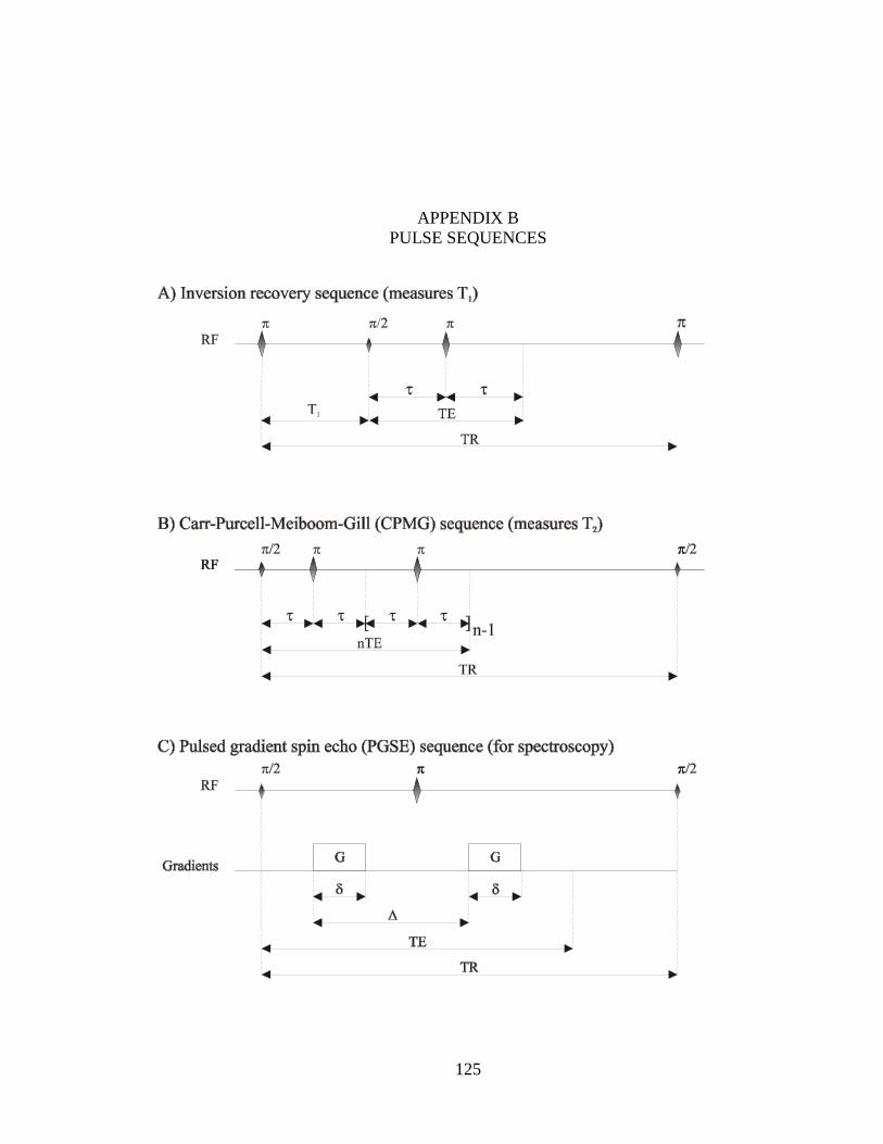
125
APPENDIX BPULSE SEQUENCES
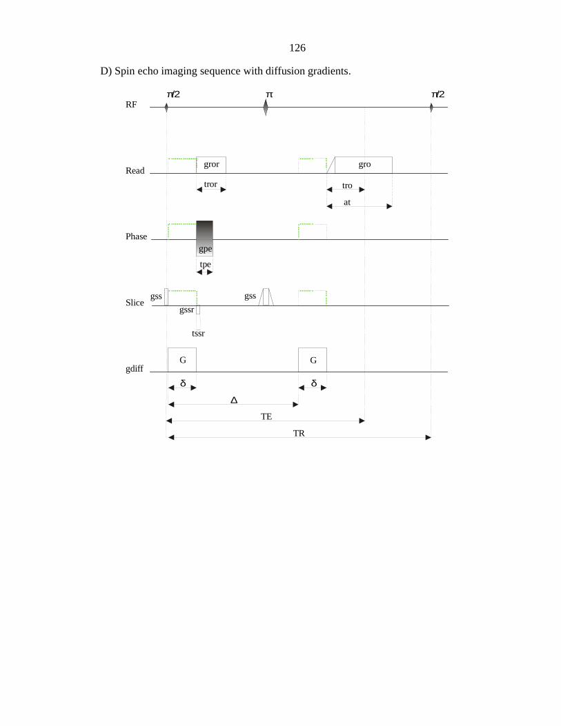
126
π/2 π π/2RF
Read
Phase
Slice
gdiff
δ δ
∆
TE
TR
G G
gssr
gpe
gror gro
gssgss
tror
tpe
tro
at
D) Spin echo imaging sequence with diffusion gradients.
tssr

APPENDIX CRAT SPINAL CORD ANATOMY AT VERTEBRAL LEVEL L1
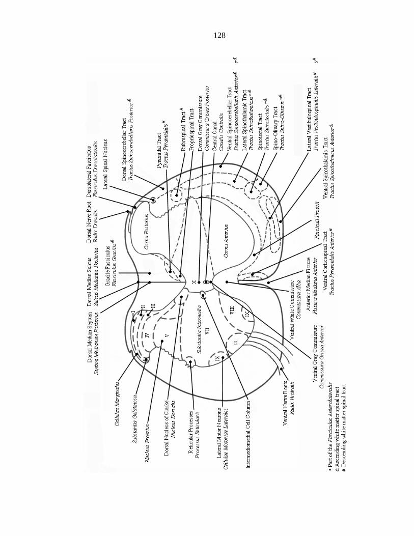
128
129
LIST OF REFERENCES
SF Akber (1996) NMR relaxation data of water proton in normal tissues. Physiol ChemPhys & Med NMR 28, 205-238.
ER Andrew (1958) “Nuclear magnetic resonance.” New York: Cambridge UniversityPress.
Y Assaf and Y Cohen (1998) Non-mono-exponential attenuation of water in n-AcetylAspartate signals due to diffusion in brain tissue. J Mag Reson 131, 69-85.
Y Baba, MM Lerch, DD Stark, A Tanimoto, BP Kreft, L Zhao, AK Saluja and MTakahashi (1994) Time after excision and temperature alter ex vivo tissuerelaxation time measurements. J Mag Reson Imaging 4, 647-651.
PJ Basser (1995) Inferring microstructural features and the physiological state of tissuesfrom diffusion-weighted images. NMR in Biomed 8, 333-344.
PJ Basser, J Mattiello and D Le Bihan (1992) Diagonal and off-diagonal components ofthe self-diffusion tensor: their relation to and estimation from the NMR spin-echosignal. Proc 11th Annual Meet. SMRM, Berlin 1:1222.
PJ Basser, J Mattiello and D Le Bihan (1994a) MR diffusion tensor spectroscopy andimaging. Biophysical J 66, 259-267.
PJ Basser, J Mattiello and D Le Bihan (1994b) Estimation of the effective self-diffusiontensor from the NMR spin echo. J Magn Reson B 103, 247-254.
PJ Basser and C Pierpaoli (1996) Microstructural and physiological features of tissueselucidated by quantitative-diffusion-tensor-MRI. J Mag Reson B 111, 209-219.
JL Becerra, WR Puckett, ED Hiester, RM Quencer, AE Marcillo, MJ Donovan Post andRP Bunge (1995) MR-Pathologic comparisons of wallerian degeneration in spinalcord injury. AJNR: Am J Neurorad 16, 125-133.
G Bodenhausen, J Kogler and RR Ernst (1984) Selection of coherence-transfer pathwaysin NMR experiments. J Mag Reson 58, 370-388.
130
GL Borgin, RJS Brown and R Fantazzini (1996) Nuclear magnetic resonance relaxivityand surface-to-volume ratio in porous media with a wide distribution of poresizes. J Appl Phys 79, 3656-3664.
EL Bossart, BA Inglis, DL Buckley, ED Wirth III and TH Mareci (1999a) Multiplecomponent diffusion tensor imaging in excised fixed CNS tissue. ISMRM 7th
Scientific Meeting and Exhibition, Philadelphia, PA 1, 328.
EL Bossart, BA Inglis, ED Wirth III and TH Mareci (1999b) Multiexponential diffusionimaging of normal and 1-month post-injury rat spinal cords. ISMRM 7th ScientificMeeting and Exhibition, Philadelphia, PA 2, 991.
PA Bottomley (1982) NMR imaging techniques and applications: a review. Rev Sc.Instrum 53, 1319-1337.
PA Bottomley, TH Forster, RE Argersinger and LM Pfeifer (1984) A review of normaltissue hydrogen NMR relaxation times and relaxation mechanisms from 1-100MHz: dependence on tissue type, NMR frequency, temperature, species, excision,and age. Med Phys 11, 425-448.
DL Buckley, JD Bui, MI Phillips, T Zelles, BA Inglis, HD Plant and SJ Blackband(1999) The effect of ouabain on water diffusion in the rat hippocampal slicemeasured by high resolution NMR imaging. Mag Reson Med 41, 137-142.
JD Bui, DL Buckley, SJ Blackband and JR Forder (1999) Biexponential diffusionobserved in myocardial tissue slices. ISMRM 7th Scientific Meeting andExhibition, Philadelphia, PA 1, 556.
PT Callaghan (1991) “Principles of NMR microscopy.” New York: Oxford UniversityPress.
D Canet and JB Robert (1991) Behavior of the NMR relaxation parameters at high fields,pp. 45-89 in “NMR at Very High Field,” P Diehl, E Fluck, H Gunther, R Kosfeld,J Seelig and JB Robert, eds. New York: Springer-Verlag.
MB Carpenter (1991) “Core Text of Neuroanatomy Fourth Edition.” Baltimore: Williamsand Wilkins.
MJ Carvlin, R Asato, DB Hackney, E Kassab and PM Joseph (1989) High-resolution MRof the spinal cord in human and rats. Am J Neuroradiol 10, 13-17.
TL Chenevert, JA Brunberg and JG Pipe (1990) Anisotropic diffusion in human whitematter: demonstration with NMR techniques in vivo. Radiology 177, 401-405.
131
R Ek, U Henriksson, C Nystrom and L Odberg (1994) Pore characterization in cellulosebeads from diffusion studies using spin echo NMR technique. PowderTechnology 81, 279-286.
HW Fischer, Y Van Haverbeke, PA Rinck, I Schmitz-Feuerhake and RN Muller (1989)The effects of aging and storage conditions on excised tissues as monitored bylongitudinal relaxation dispersion profiles. Mag Reson Med 9, 315-324.
JC Ford, DB Hackney, DC Alsop, H Jara, PM Joseph, CM Hand and P Black (1994)MRI characterization of diffusion coefficients in a rat spinal cord injury model.Mag Reson Med 31, 488-494.
V Gulani, GA Iwamoto, H Jiang, JS Shimony, AG Webb and PC Lauterbur (1997) Amultiple echo pulse sequence for diffusion tensor imaging and its application inexcised rat spinal cord. Mag Reson Med 38, 868-873.
Z Gyorffy-Wagner, E Englund, E-M Larson, A Brun, S Cronqvist and B Persson (1986)Proton magnetic resonance relaxation times T1 and T2 related to postmorteminterval. Acta Radiol Diag 27, 115-118.
I Hahnenstein, M Albert, H Hasse, CG Kreiter and G Maurer (1995) NMR spectroscopicand densimetric study of reaction-kinetics of formaldehyde polymer formation inwater, deuterium-oxide, and methanol. Indus Eng Chem Res 34, 440-450.
I Hahnenstein, H Hasse, CG Kreiter and G Maurer (1994) H-1-NMR and C-13-NMRspectroscopic study of chemical-equilibria in solutions of formaldehyde in water,deuterium-oxide, and methanol. Indus Eng Chem Res 33, 1022-1029.
KG Helander (1994) Kinetic studies of formaldehyde binding in tissue. Biotech andHistochem 69, 177-179.
KG Helmer, BJ Dardzinski and CH Sotak (1995) The application of porous-media theoryto the investigation of time-dependent diffusion in In Vivo systems. NMR inBiomed 8, 297-306.
KG Helmer, MD Silva, O Oreg-Mayzel and CH Sotak (1999) Deconvolution ofrestriction effects compartmental diffusion using relaxography and diffusionmeasurements. 40th Experimental Nuclear Magnetic Resonance Conference, Feb.28 – Mar. 5 1999, Orlando, FL, abstract 169, p.188.
WS Hinshaw and AH Lent (1983) An introduction to NMR imaging: from the Blochequation to the imaging equation. Proc of the IEEE 71, 338-.
D Hopwood (1972) Theoretical and practical aspects of gluteraldehyde fixation.Histochem J 4, 267-303.
132
BA Inglis, L Yang, ED Wirth III, D Plant and TH Mareci (1997) Diffusion anisotropy inexcised normal rat spinal cord measured by NMR microscopy. Mag ResonImaging 15, 441-450.
A Jayakrishnan and SR Jameela (1996) Gluteraldehyde as a fixative in bioprostheses anddrug delivery matrices. Biomaterials 17, 471-484.
RL Kamman, KG Go, GP Stomp, CE Hulstaert and HJC Berendsen (1985) Changes ofrelaxation times T1 and T2 in rat tissues after biopsy and fixation. Mag ResonImaging 3, 245-250.
JI Kaplan and G Fraenkel (1980) “NMR of Chemically Exchanging Systems.” NewYork: Academic Press.
J Karger, H Pfeifer and W Heink (1988) Principles and application of self-diffusionmeasurements by NMR. Adv Mag Reson 12, 1-89.
J Kawahara, T Ohmori, T Ohkubo, S Hattori and M Kawamura (1992) The structure ofgluteraldehyde in aqueous-solution determined by ultraviolet-absorption andlight-scattering. Anal Biochem 201, 94-98.
RP Kennan, KA Richardson, JH Zhong, MJ Maryanski and JC Gore (1996) The effectsof cross-link density and chemical exchange on magnetization transfer inpolyacrylamide gels. J Mag Reson B 110, 267-277.
CF Kirsch, M Neeman, KR Halliday and LO Sillerud (1991) NMR microscopy anddiffusion anisotorpy of experimental spinal cord trauma. 10th Annual Meet.SMRM, San Fransisco 1, 1261.
F Kraemaer, A Darquie, CA Clark and D Le Bihan (1999) Separation of two diffusioncompartments in the human brain. ISMRM 7th Scientific Meeting and Exhibition,Philadelphia, PA 3, 1808.
LL Latour, PP Mitra, RL Kleinberg and CH Sotak (1993) Time-dependent diffusioncoefficient of fluids in porous media as a probe of surface-to-volume ratio. J MagReson A 101, 342-346.
LL Latour, K Svoboda, PP Mitra and CH Sotak (1994) Time-dependent diffusion ofwater in a biological model system. Proc Natl Acad Sci USA 91, 1229-1233.
PC Lauterbur (1973) Image formation by induced local interactions; Examplesemploying nuclear magnetic resonance. Nature 242, 190-191.
D Le Bihan and E Breton (1985) Imagerie de diffusion in-vivo par resonance magnetiquenucleaire. Cr Acad Sci 301, 1109-1112.
133
D Le Bihan, R Turner and P Douek (1993) Is water diffusion restricted in human brainwhite matter? An echo planar NMR imaging study. NeuroReport 4, 887-890.
R Lenk (1986) “Fluctuations, Diffusion and Spin Relaxation.” New York: Elsevier.
JG Li, GJ Stanisz and RM Henkelman (1998) Integrated analysis of diffusion andrelaxation of water in blood. Mag Reson Med 40, 79-88.
TH Mareci (1988) Principles of multiple-quantum spectroscopy, in “Pulse methods in 1Dand 2D liquid-phase NMR,” WD Brey, ed. New York: Academic Press.
J Mattiello, PJ Basser and D Le Bihan (1994) Analytical expressions for the b matrix inNMR diffusion imaging and spectroscopy. J Mag Reson A 108, 131-141
PP Mitra, PN Sen and LM Schwartz (1993) Short-time behavior of the diffusioncoefficient as a geometrical probe of porous media. Phys Rev B 47, 8565-8574.
PP Mitra, PN Sen, LM Schwartz and P Le Doussal (1992) Diffusion propagator as aprobe of the structure of porous media. Phys Rev Letters 68, 3555-3558.
DC Montgomery (1976) “Design and Analysis of Experiments,” New York: Wiley,Chapter 13.
ME Moseley, Y Cohen, J Kucharczyk, J Mintorovitch, HS Asgari, MF Wardland, JTsuruda and D Norman (1990) Diffusion-weighted MR imaging of anisotropicdiffusion in cat central nervous system. Radiology 176, 439-445.
ME Moseley, MC Nishimura, LH Pitts, HM Bartkowski and TL James (1984) Protonnuclear magnetic resonance spectroscopy of normal and edematous brain tissue invitro: changes in relaxation during tissue storage. Mag Reson Imaging 2, 205-209.
RV Mulkern, HP Zengingonul, D Holtzman, CRG Guttmann, RL Robertson, WKyriakos, JA Jolesz and SE Maier (1999) Multi-component apparent diffusioncoefficients in human brain: gray/white matter differences and spin-latticerelaxation times. ISMRM 7th Scientific Meeting and Exhibition, Philadelphia, PA3, 1806.
H Nagara, T Inoue, T Koga, T Kitaguchi, J Tateishi and I Goto (1987) Formalin fixedbrains are useful for magnetic resonance imaging (MRI) study. J Neurol Sci 81,67-77.
C Nicholson and E Sykova (1998) Extracellular space structure revealed by diffusionanalysis. Trends Neurosci 21, 207-215.
134
T Niendorf, RM Dijkhuizen, DG Norris, M van Lookeren Campagne and K Nicolay(1996) Biexponential diffusion attenuation in various states of brain tissue:Implications for diffusion-weighted imaging. Mag Reson Med 36, 847-857.
DG Norris and T Niendorf (1995) Interpretation of DW-NMR data: dependence onexperimental conditions. NMR in Biomed 8, 280-288.
DG Norris, T Niendorf and D Leibfritz (1994) Healthy and infarcted brain tissues studiedat short diffusion times: the origins of apparent restriction and the reduction inapparent diffusion coefficient. NMR in Biomed 7, 304-310.
J Ono, K Harada, N Takahashi, M Maeda, K Ikenaka, K Sakurai, N Sakai, T Kagawa, BFritz-Zieroth, T Nagai, A Nihei, S Hashimoto and S Okada (1995) Differentiationbetween dysmyelination and demyelination using magnetic resonance diffusionalanisotropy. Brain Res 671, 141-148.
PM Pattany, WR Puckett, KJ Klose, RM Quencer, RP Bunge, L Kasubuski and RGWalker (1997) High-resolution diffusion-weighted MR of fresh and fixed catspinal cords: evaluation of diffusion coefficients and anisotropy. Am JNeuroradiol 18, 1049-1056.
J Pfeuffer, SW Provencer and R. Gruetter (1999) Water diffusion in rat brain in vivo asdetected at very large b values is multicompartmental. ISMRM 7th ScientificMeeting and Exhibition, Philadelphia, PA 1, 557.
C Pierpaoli and PJ Basser (1996) Toward a quantitative assessment of diffusionanisotropy. Mag Reson Med 36, 893-904.
C Pierpaoli, P Jezzard, PJ Basser, A Barnett and G DiChiro (1996) Diffusion Tensor MRImaging of the Human Brain. Radiology 201, 637-648.
P Prento (1995) Gluteraldehyde for electron-microscopy – a practical investigation ofcommercial gluteraldehydes and gluteraldehyde-storage conditions.Hisotchemical J 27, 906-913.
JS Schoeniger, N Aiken, E Hsu and SJ Blackband (1994) Relaxation-time and diffusionNMR microscopy of single neurons. J Mag Reson B 103, 261-273.
GJ Stanisz and RM Henkelman (1998) Diffusional anisotropy of T2 components inbovine optic nerve. Mag Reson Med 40, 405-410.
GJ Stanisz, A Szafer, GA Wright and RM Henkelman (1997) An analytical model ofrestricted diffusion in bovine optic nerve. Mag Reson Med 37, 103-111.
EO Stejskal (1965) Use of spin echoes in a pulsed magnetic-field gradient to studyanisotropic, restricted diffusion and flow. J Chem Phys 43, 3597-3603.
135
EO Stejskal and JE Tanner (1965) Spin diffusion measurements: spin echos in thepresence of time-dependent field gradients. J Chem Phys 42, 288-292.
E Sykova (1997) The extracellular space in the CNS: Its regulation, volume andgeometry in normal and pathological neuronal function. The Neuroscientist 3, 28-41.
E Sykova, L Vargova, S Prokopova and Z Simonova (1999) Glial swelling andastrogliosis produce diffusion barriers in the rat spinal cord. Glia 25, 56-70.
A Szafer, J Zhong and JC Gore (1995a) Theoretical model for water diffuison in tissues.Mag Reson Med 33, 697-712.
A Szafer, J Zhong and JC Gore (1995b) Diffusion-weighted imaging in tissues:theoretical models. NMR in Biomed 8, 289-296.
DI Thickman, HL Kundel and G Wolf (1983) Nuclear magnetic resonance characteristicsof fresh and fixed tissue: the effect of elapsed time. Radiology 148, 183-185.
C Thompson, O Henriksen and P Ring (1987) In vivo measurements of water self-diffusion in the human brain by magnetic resonance imaging. Acta Radiol Scand28, 353-361.
HC Torrey (1956) Bloch equations with diffusion terms. Phys Rev 104, 563-.
M Tovi and A Ericsson (1992) Measurements of T1 and T2 over time in formalin-fixedhuman whole-brain specimens. Acta Radiol 33, 400-404.
R Tycko (1994) How does nuclear magnetic resonance probe molecular dynamics, in“Nuclear Magnetic Resonance Probes of Molecular Dynamics,” R. Tycko, ed.Boston: Kluwer.
D van Dusschoten, P Adric De Jager and H van As (1995) Extracting diffusion constantsfrom echo-time-dependent PFG NMR data using relaxation-time information. JMag Reson A 116, 22-28.
P van Gelderen, MHM de Vleeschouwer, D DesPres, J Pekar, PCM van Zijl and CTWMoonen (1994) Water diffusion in acute stroke. Mag Reson Med 31, 154-163.
PCM van Zijl, CTW Moonen, P Faustino, J Pekar, O Kaplan and JS Cohen (1991)Complete separation of intracellular and extracellular information in NMR spectraof perfused cells by diffusion-weighted spectroscopy. Proc Natl Acad Sci USA88, 3228-3232.
136
RE Wasylichen (1987) NMR Relaxation and Dynamics, in “NMR SpectroscopyTechniques,” C Dybowske and RL Lichter, eds. New York: Marcel Dekker Inc.
MR Willcott (1984) Comparison of in vivo and in vitro NMR relaxation times. Prog NuclMed 8, 62-64.
L Yang, BA Inglis, S Yang and TH Mareci (1994) A building-block approach to theanalysis of generalized gradient weighting: application to diffusion tensormeasurements. 35th Experimental Nuclear Magnetic Resonance Conference, April1994, Pacific Grove, CA, abstract MP113, p.143.
137
BIOGRAPHICAL SKETCH
Elizabeth L. Bossart was born in Cincinnati, OH and raised in Texas. After
completing high school in Houston, she headed, on scholarship, for Southwestern
University in Georgetown, TX, to pursue degrees in biology and chemistry, or so she
thought. After a year in the program she changed her majors to physics and mathematics,
where she happily remained for her final three years as an undergraduate. She was
awarded a physics scholarship in her final two years of undergraduate study, and also
earned the highest honor for a student studying physics at Southwestern, the Golden
Eagle Award. Also during her undergraduate career, she spent two summers at the North
Carolina State University Department of Physics in a National Science Foundation
sponsored summer research program. This taste of research showed her that she enjoyed
it, and with that experience she decided to pursue her doctorate in physics. She was
awarded a US Department of Energy fellowship at the University of Florida for her first
two years of graduate study, after which she began work in the lab of Dr. T.H. Mareci,
doing studies of water self-diffusion in tissue using magnetic resonance techniques. Her
hope for the future is to continue learning and growing through both research and
teaching.