Earth Planets Space, 60, 937–948, 2008

Magnetic poles and dipole tilt variation over the past decades to millennia

M. Korte and M. Mandea

GeoForschungsZentrum Potsdam, Telegrafenberg, 14473 Potsdam, Germany

(Received December 6, 2007; Revised July 2, 2008; Accepted August 2, 2008; Online published October 15, 2008)

Due to the strong dipolar character of the geomagnetic field the shielding effect against cosmic and solar rayparticles is weakest in the polar regions. We here present a comprehensive study of the evolution of magneticand geomagnetic pole locations and the Earth’s magnetic core field in both polar regions over the past few yearsto millennia. North and south magnetic poles change independently according to the asymmetric complexity ofthe field in the two hemispheres, and the changes are not correlated to variations of the dipole axis. The recent,strong acceleration of the north magnetic pole motion appears to be linked to a reverse flux patch at the core-mantle boundary, and an increasing deceleration of the pole over the next years seems likely. Over the wholestudied period of 7000 years two periods of comparatively high velocity of the north magnetic pole are observedat 4500 BC and 1300 BC, based on the presently available data and models. Geographic latitudes and longitudesof magnetic and geomagnetic poles based on the studied geomagnetic field models are available together withanimations of the poles and polar field behaviour from our webpage http://www.gfz-potsdam.de/geomagnetic-field/poles.Key words: Geomagnetic field, magnetic poles, dipole axis.

1. IntroductionThe geomagnetic main field, generated in the Earth’s

outer fluid core, is constantly changing, this temporal vari-ation being known as secular variation. At and above theEarth’s surface the observed time scales of secular variationrange from about one year (geomagnetic jerks) to millionsof years, where extreme events like excursions and polarityreversals occur. The field is approximately dipole-shaped inthe near-Earth environment. Recently, a strong decrease ofthe dipole moment, persisting at least since the beginning ofsystematic, full vector field measurements around 1830, hasraised attention (Gubbins, 1987; Hulot et al., 2002; Olson,2002; Constable and Korte, 2006; Gubbins et al., 2006).Another feature of the field is currently showing quite ex-treme changes, and this is the magnetic north pole location(Newitt et al., 2002). Since about 1970 its velocity hassuddenly increased to almost 60 km/yr, much higher thanthe average observed over the past centuries (Mandea andDormy, 2003).

The polar regions are the areas where incoming cosmicand solar wind particles, being deflected by and followingthe geomagnetic field lines, penetrate most deeply into theatmosphere. Connections between geomagnetic field andclimate changes have once again become discussed contro-versially lately (Courtillot et al., 2007; Bard and Delaygue,2007). If mechanisms like galactic cosmic rays influencingcloud cover play a role, then the location of the geomag-netic field poles, particularly with regard to latitude and/orrelative to land mass, might be important in terms of cli-

Copyright c© The Society of Geomagnetism and Earth, Planetary and Space Sci-ences (SGEPSS); The Seismological Society of Japan; The Volcanological Societyof Japan; The Geodetic Society of Japan; The Japanese Society for Planetary Sci-ences; TERRAPUB.

matological effects. The behaviour of the magnetic polesis investigated in the present study together with the gen-eral main field behaviour in the polar regions. Part of ourmotivation also comes from the recently increased interestin the Arctic and Antarctic during the International PolarYear (IPY) which started in March 2007.

Two sets of poles are defined with respect to the magneticfield, the magnetic and the geomagnetic poles, with charac-teristics summarised in the following. The magnetic poleor dip pole positions are the areas where the field lines pen-etrate the Earth vertically, i.e. the inclination reaches 90◦.Due to the non-dipole influences in the core field, north(NMP) and south (SMP) magnetic poles are not diametri-cally opposed. Their locations can be determined in twoways, by direct measurements or from global geomagneticfield models. Direct observations involve costly expedi-tions to inhospitable areas, as currently the NMP is situ-ated far away on the icy Arctic Ocean, and the SMP is inthe Ocean, just off the Antarctic coast and south of Aus-tralia (see Fig. 1). Measurements can be influenced by localcrustal field anomalies. Moreover, due to the strong influ-ence of external magnetic field contributions at high geo-magnetic latitudes the magnetic pole locations are not fixedpoints, but move within a radius of a couple of km up to100 km per day, depending on geomagnetic activity (Daw-son and Newitt, 1982). For this reason, measurements todetermine the magnetic poles of the core field have to beproperly designed to account not only for the specific con-ditions in the Arctic and Antarctic regions, but also for thehigh variability of the vertical field lines locations. Eightdirect measurements of the pole locations for the northernhemisphere have been carried out (1831, 1905, 1947, 1962,1973, 1984, 1994 and 2001, see Newitt and Barton, 1996;

937

938 M. KORTE AND M. MANDEA: MAGNETIC AND GEOMAGNETIC POLES

1590

20061590

2006

1590

2006

15902006

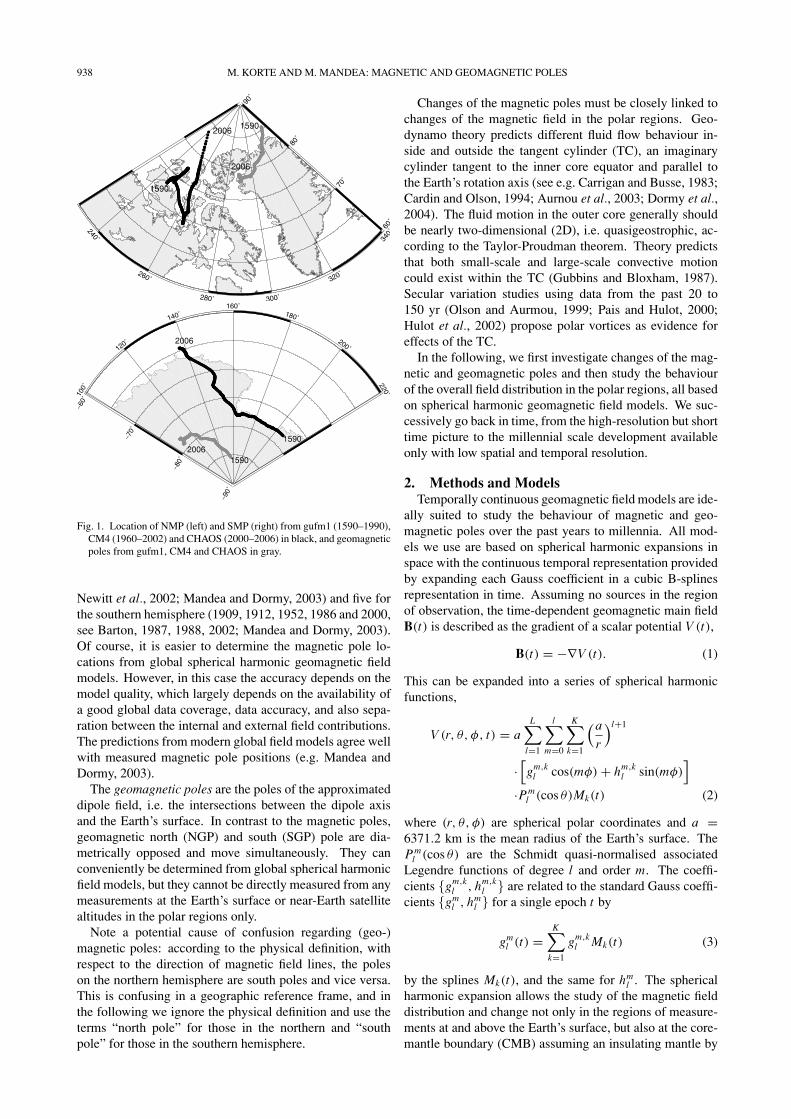
Fig. 1. Location of NMP (left) and SMP (right) from gufm1 (1590–1990),CM4 (1960–2002) and CHAOS (2000–2006) in black, and geomagneticpoles from gufm1, CM4 and CHAOS in gray.

Newitt et al., 2002; Mandea and Dormy, 2003) and five forthe southern hemisphere (1909, 1912, 1952, 1986 and 2000,see Barton, 1987, 1988, 2002; Mandea and Dormy, 2003).Of course, it is easier to determine the magnetic pole lo-cations from global spherical harmonic geomagnetic fieldmodels. However, in this case the accuracy depends on themodel quality, which largely depends on the availability ofa good global data coverage, data accuracy, and also sepa-ration between the internal and external field contributions.The predictions from modern global field models agree wellwith measured magnetic pole positions (e.g. Mandea andDormy, 2003).

The geomagnetic poles are the poles of the approximateddipole field, i.e. the intersections between the dipole axisand the Earth’s surface. In contrast to the magnetic poles,geomagnetic north (NGP) and south (SGP) pole are dia-metrically opposed and move simultaneously. They canconveniently be determined from global spherical harmonicfield models, but they cannot be directly measured from anymeasurements at the Earth’s surface or near-Earth satellitealtitudes in the polar regions only.

Note a potential cause of confusion regarding (geo-)magnetic poles: according to the physical definition, withrespect to the direction of magnetic field lines, the poleson the northern hemisphere are south poles and vice versa.This is confusing in a geographic reference frame, and inthe following we ignore the physical definition and use theterms “north pole” for those in the northern and “southpole” for those in the southern hemisphere.

Changes of the magnetic poles must be closely linked tochanges of the magnetic field in the polar regions. Geo-dynamo theory predicts different fluid flow behaviour in-side and outside the tangent cylinder (TC), an imaginarycylinder tangent to the inner core equator and parallel tothe Earth’s rotation axis (see e.g. Carrigan and Busse, 1983;Cardin and Olson, 1994; Aurnou et al., 2003; Dormy et al.,2004). The fluid motion in the outer core generally shouldbe nearly two-dimensional (2D), i.e. quasigeostrophic, ac-cording to the Taylor-Proudman theorem. Theory predictsthat both small-scale and large-scale convective motioncould exist within the TC (Gubbins and Bloxham, 1987).Secular variation studies using data from the past 20 to150 yr (Olson and Aurmou, 1999; Pais and Hulot, 2000;Hulot et al., 2002) propose polar vortices as evidence foreffects of the TC.

In the following, we first investigate changes of the mag-netic and geomagnetic poles and then study the behaviourof the overall field distribution in the polar regions, all basedon spherical harmonic geomagnetic field models. We suc-cessively go back in time, from the high-resolution but shorttime picture to the millennial scale development availableonly with low spatial and temporal resolution.

2. Methods and ModelsTemporally continuous geomagnetic field models are ide-

ally suited to study the behaviour of magnetic and geo-magnetic poles over the past years to millennia. All mod-els we use are based on spherical harmonic expansions inspace with the continuous temporal representation providedby expanding each Gauss coefficient in a cubic B-splinesrepresentation in time. Assuming no sources in the regionof observation, the time-dependent geomagnetic main fieldB(t) is described as the gradient of a scalar potential V (t),

B(t) = −∇V (t). (1)

This can be expanded into a series of spherical harmonicfunctions,

V (r, θ, φ, t) = aL∑

l=1

l∑m=0

K∑k=1

(a

r

)l+1

·[gm,k

l cos(mφ) + hm,kl sin(mφ)

]·Pm

l (cos θ)Mk(t) (2)

where (r, θ, φ) are spherical polar coordinates and a =6371.2 km is the mean radius of the Earth’s surface. ThePm

l (cos θ) are the Schmidt quasi-normalised associatedLegendre functions of degree l and order m. The coeffi-cients {gm,k

l , hm,kl } are related to the standard Gauss coeffi-

cients {gml , hm

l } for a single epoch t by

gml (t) =

K∑k=1

gm,kl Mk(t) (3)

by the splines Mk(t), and the same for hml . The spherical

harmonic expansion allows the study of the magnetic fielddistribution and change not only in the regions of measure-ments at and above the Earth’s surface, but also at the core-mantle boundary (CMB) assuming an insulating mantle by

M. KORTE AND M. MANDEA: MAGNETIC AND GEOMAGNETIC POLES 939

simple downward continuation via the relation of the radii((ar

)l+1)

.

We consider four continuous field models in this study toinvestigate pole and field changes over different time-scales.

• CHAOS is the first continuous model based on satel-lite data only, covering the time interval from March1999 to December 2005 (Olsen et al., 2006). Thename represents the three satellites which have pro-vided data: CHAMP, Ørsted, SAC-C. The CHAOSmodel describes the core field and its secular varia-tion with the highest possible spatial and temporal res-olution. The core field is fully resolved up to degreeswhere its contribution is hidden by the crustal field.Secular variation is reliably resolved up to sphericalharmonic degree and order 15, unprecedented by anyother continuous field model. The knot-point spacingof the splines is 1 yr.

• CM4, the Comprehensive Model (4th generation), isan attempt to describe all field contributions in onemodel, from core, lithosphere, sources external to theEarth and their induced counterparts (Sabaka et al.,2004). It covers the time span 1960 to mid-2002 with aspline knot-point spacing of 2.5 yrs. This model can beuseful for separating certain contributions of the quiettime magnetic field. Here, we only consider the corefield and its secular variation given by this model.

• Gufm1 goes as far back in time as direct magneticfield measurements allow, covering the interval 1590to 1990 (Jackson et al., 2000) with spline knot-pointsevery 2.5 yrs. This is the latest achievement of the pi-oneering work by Bloxham and Jackson (1992) to de-velop spline-based continuous models, which also areparticularly useful for studying the geomagnetic fieldat the CMB. In order not to include artificial structurecaused by data errors and insufficient data coverage, aregularisation has been applied in the modelling. Theresult is a smoother model which shows the minimumamount of structure necessary to explain the used data.As a consequence, the spatial resolution of this modelclearly changes and improves with time due to increas-ing amounts of (better) data. Comparing geomagneticpower spectra we estimate the reliable spatial resolu-tion of main field and secular variation to increase fromabout degree 6 and 5, respectively, in 1590 to 10 (mainfield) and 7 (secular variation) for the last years of themodel.

• CALS7K.2, a Continuous model based on Archaeo-magnetic and Lake Sediment data of the past 7 kyr, isone of the first attempts to extend continuous globalfield models towards paleomagnetic time-scales withresolution beyond the quadrupole contribution (Korteand Constable, 2005a). Although the modelling tech-nique is nearly the same as for gufm1, the resolutionis severely limited by the inferior data distribution anduncertainties in the archaeo- and paleomagnetic dataand their dating, which are much higher than even inhistorical direct field observations. A similar regular-isation as in gufm1 has been applied and the reliablespatial resolution of this model is about spherical har-

monic degree 4 to 5, while the temporal resolution isno better than 50 to 100 yr (spline knot-points are sep-arated by about 50 yrs).

Geomagnetic north pole longitude φ and latitude λ areconveniently found from spherical harmonic dipole coeffi-cients g0

1, g11 and h1

1 following Langel (1987)

tan φ = h11

g11

, (4)

and

λ = 90◦ − θ,

cos θ = g01

m,

(5)

with

m =√(

g01

)2 + (g1

1

)2 + (h1

1

)2. (6)

Geomagnetic south pole locations are obtained straight-forwardly as the diametrically opposed points. Magneticpoles predicted by the models are found by evaluating thefull core field description in the north and south polar re-gions and finding the locations where inclination valuesare 90◦. The velocity, v(t) of the pole movement at timet = (t1 + t2)/2 is calculated as

v(t) =

([(λ(t2) − λ(t1))

2π Rpol

360◦

]2

+[(φ(t2) − φ(t1))

2π Req

360◦ cos(λ(t2))

]2) 1

2

t2 − t1,

(7)

with Rpol = 6356.8 km and Req = 6378.2 km the polar andequatorial radius of the Earth, respectively.

Computer-readable ASCII files with geographic latitudesand longidutes of all the magnetic and geomagnetic pole lo-cations discussed in this work are provided on our webpagehttp://www.gfz-potsdam.de/geomagnetic-field/poles.

3. Migration of the Magnetic and GeomagneticPoles

In the following we first describe the behaviour of the ge-omagnetic (i.e. dipole axis) poles, and then of the magneticpoles, for the last four centuries coverd by models based ondirect field observations (Section 3.1). The same is done forthe past 7 millennia, when only indirect data can be used formodelling, in Section 3.2.3.1 From decades to centuries

The changes of magnetic and geomagnetic pole positionssince 1590 are shown in Fig. 1. The corresponding ve-locities together with latitudinal and longitudinal changesare given in Fig. 2. The dipole axis has been tilting awayfrom the geographical axis for most of the time, whileturning slightly westward in the northern hemisphere. Be-tween 1800 and 1950 its latitude remained nearly constantand for the past five decades the axis tilt has been slowlydecreasing. The velocity of this movement has generallyslightly decreased between 1590 and 1900 and increasedafterwards, possibly somewhat correlated to increasing and

940 M. KORTE AND M. MANDEA: MAGNETIC AND GEOMAGNETIC POLES

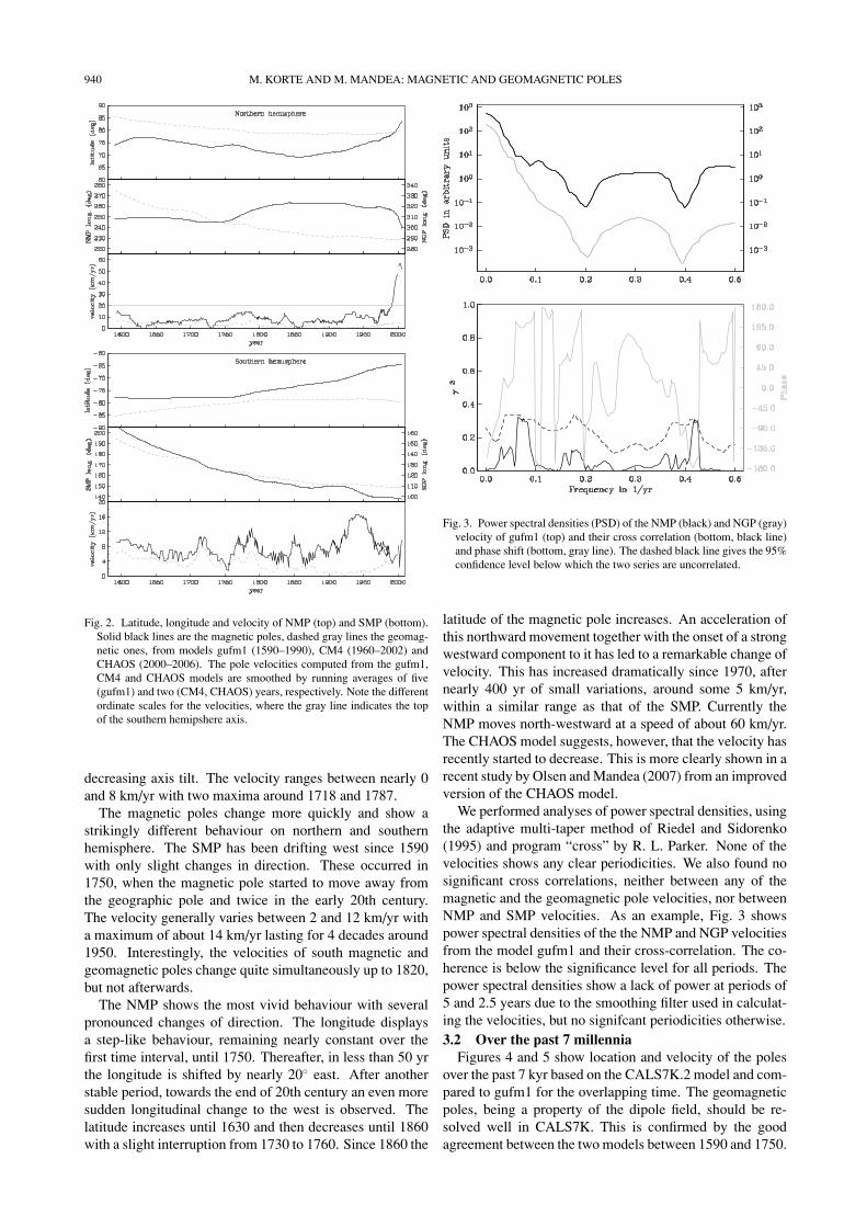
Fig. 2. Latitude, longitude and velocity of NMP (top) and SMP (bottom).Solid black lines are the magnetic poles, dashed gray lines the geomag-netic ones, from models gufm1 (1590–1990), CM4 (1960–2002) andCHAOS (2000–2006). The pole velocities computed from the gufm1,CM4 and CHAOS models are smoothed by running averages of five(gufm1) and two (CM4, CHAOS) years, respectively. Note the differentordinate scales for the velocities, where the gray line indicates the topof the southern hemipshere axis.

decreasing axis tilt. The velocity ranges between nearly 0and 8 km/yr with two maxima around 1718 and 1787.

The magnetic poles change more quickly and show astrikingly different behaviour on northern and southernhemisphere. The SMP has been drifting west since 1590with only slight changes in direction. These occurred in1750, when the magnetic pole started to move away fromthe geographic pole and twice in the early 20th century.The velocity generally varies between 2 and 12 km/yr witha maximum of about 14 km/yr lasting for 4 decades around1950. Interestingly, the velocities of south magnetic andgeomagnetic poles change quite simultaneously up to 1820,but not afterwards.

The NMP shows the most vivid behaviour with severalpronounced changes of direction. The longitude displaysa step-like behaviour, remaining nearly constant over thefirst time interval, until 1750. Thereafter, in less than 50 yrthe longitude is shifted by nearly 20◦ east. After anotherstable period, towards the end of 20th century an even moresudden longitudinal change to the west is observed. Thelatitude increases until 1630 and then decreases until 1860with a slight interruption from 1730 to 1760. Since 1860 the

Fig. 3. Power spectral densities (PSD) of the NMP (black) and NGP (gray)velocity of gufm1 (top) and their cross correlation (bottom, black line)and phase shift (bottom, gray line). The dashed black line gives the 95%confidence level below which the two series are uncorrelated.

latitude of the magnetic pole increases. An acceleration ofthis northward movement together with the onset of a strongwestward component to it has led to a remarkable change ofvelocity. This has increased dramatically since 1970, afternearly 400 yr of small variations, around some 5 km/yr,within a similar range as that of the SMP. Currently theNMP moves north-westward at a speed of about 60 km/yr.The CHAOS model suggests, however, that the velocity hasrecently started to decrease. This is more clearly shown in arecent study by Olsen and Mandea (2007) from an improvedversion of the CHAOS model.

We performed analyses of power spectral densities, usingthe adaptive multi-taper method of Riedel and Sidorenko(1995) and program “cross” by R. L. Parker. None of thevelocities shows any clear periodicities. We also found nosignificant cross correlations, neither between any of themagnetic and the geomagnetic pole velocities, nor betweenNMP and SMP velocities. As an example, Fig. 3 showspower spectral densities of the the NMP and NGP velocitiesfrom the model gufm1 and their cross-correlation. The co-herence is below the significance level for all periods. Thepower spectral densities show a lack of power at periods of5 and 2.5 years due to the smoothing filter used in calculat-ing the velocities, but no signifcant periodicities otherwise.3.2 Over the past 7 millennia

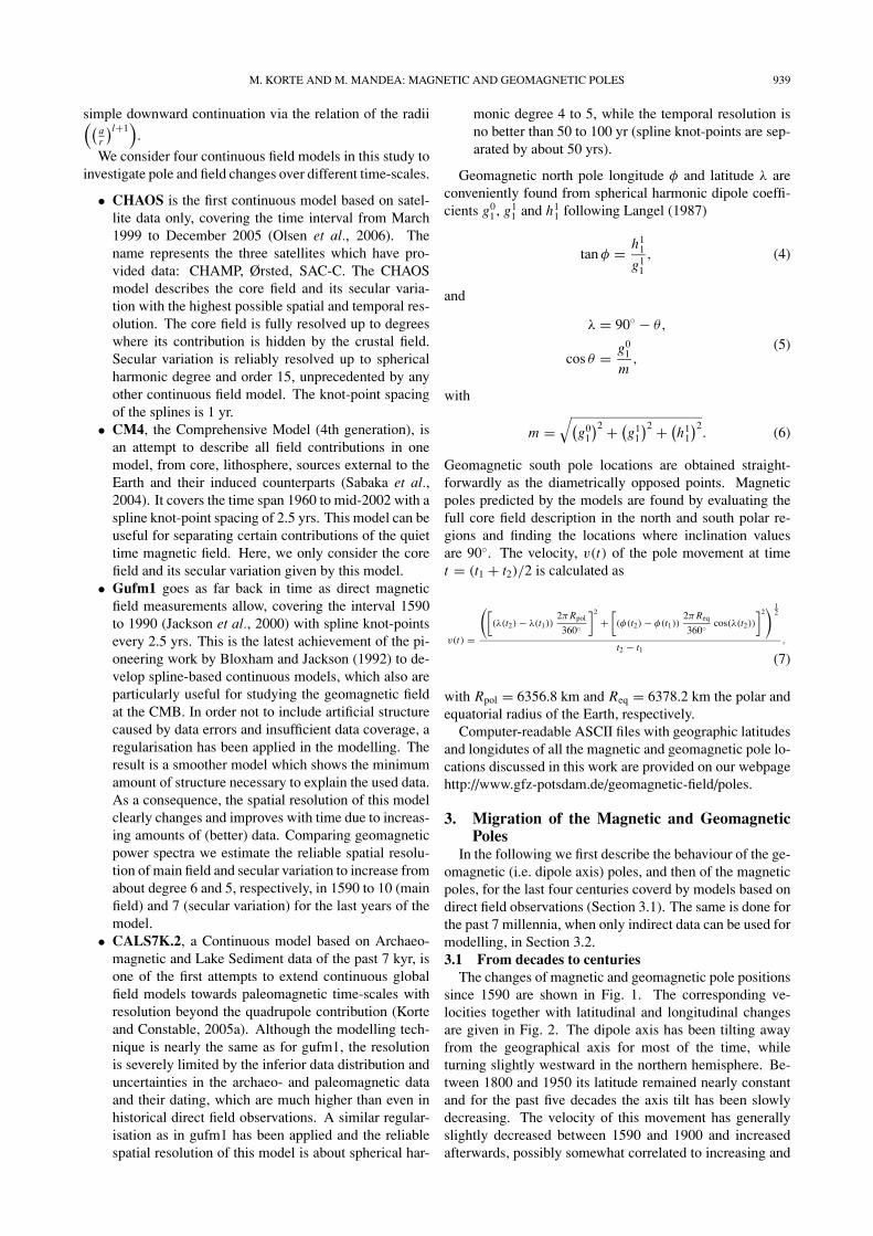
Figures 4 and 5 show location and velocity of the polesover the past 7 kyr based on the CALS7K.2 model and com-pared to gufm1 for the overlapping time. The geomagneticpoles, being a property of the dipole field, should be re-solved well in CALS7K. This is confirmed by the goodagreement between the two models between 1590 and 1750.

M. KORTE AND M. MANDEA: MAGNETIC AND GEOMAGNETIC POLES 941

-2800

-2200

-1900-1500

-1200

-1000

-2750

-2600

-2350-2100

-1000

-1800

-1450-1200

-1900-1900-1000-1000

-3000-3000

3000 BC - 1000 BC

-3600

-5000-4600

-4300

-3000-3400

5000 BC - 3000 BC

-4100-5000

-4800

-4100

-3000-3200

-3850

-4450-4600-5000 -3900

1000 BC - AD 1000

-350

-1000

-500800

0

1000 -1000

1000

250-400

800

-750

1000

-600

-350

-150

600

200

AD 1000 - 1950

1000

1400

1750

19501590

1860

1650

19501000

15901950

17501590

1990

1760

1920

1000

19501300

1600

1000

1950

1950

1150 1350

1550 1750

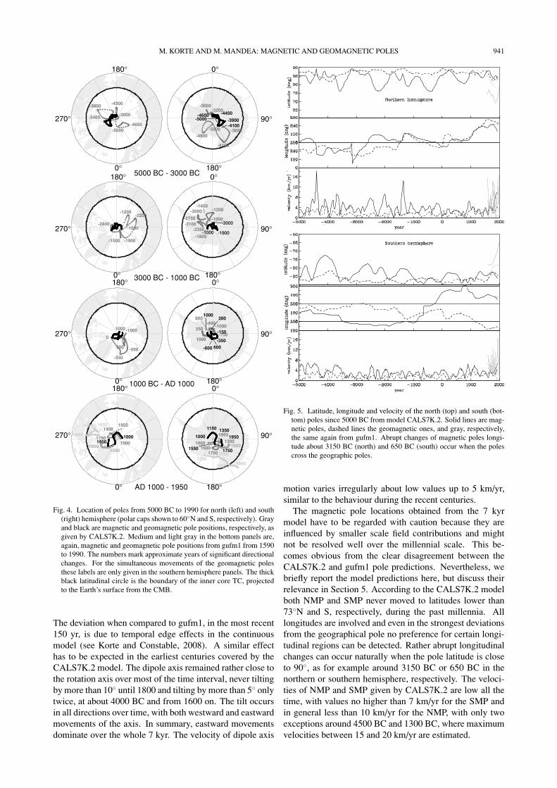
Fig. 4. Location of poles from 5000 BC to 1990 for north (left) and south(right) hemisphere (polar caps shown to 60◦N and S, respectively). Grayand black are magnetic and geomagnetic pole positions, respectively, asgiven by CALS7K.2. Medium and light gray in the bottom panels are,again, magnetic and geomagnetic pole positions from gufm1 from 1590to 1990. The numbers mark approximate years of significant directionalchanges. For the simultaneous movements of the geomagnetic polesthese labels are only given in the southern hemisphere panels. The thickblack latitudinal circle is the boundary of the inner core TC, projectedto the Earth’s surface from the CMB.

The deviation when compared to gufm1, in the most recent150 yr, is due to temporal edge effects in the continuousmodel (see Korte and Constable, 2008). A similar effecthas to be expected in the earliest centuries covered by theCALS7K.2 model. The dipole axis remained rather close tothe rotation axis over most of the time interval, never tiltingby more than 10◦ until 1800 and tilting by more than 5◦ onlytwice, at about 4000 BC and from 1600 on. The tilt occursin all directions over time, with both westward and eastwardmovements of the axis. In summary, eastward movementsdominate over the whole 7 kyr. The velocity of dipole axis

Fig. 5. Latitude, longitude and velocity of the north (top) and south (bot-tom) poles since 5000 BC from model CALS7K.2. Solid lines are mag-netic poles, dashed lines the geomagnetic ones, and gray, respectively,the same again from gufm1. Abrupt changes of magnetic poles longi-tude about 3150 BC (north) and 650 BC (south) occur when the polescross the geographic poles.

motion varies irregularly about low values up to 5 km/yr,similar to the behaviour during the recent centuries.

The magnetic pole locations obtained from the 7 kyrmodel have to be regarded with caution because they areinfluenced by smaller scale field contributions and mightnot be resolved well over the millennial scale. This be-comes obvious from the clear disagreement between theCALS7K.2 and gufm1 pole predictions. Nevertheless, webriefly report the model predictions here, but discuss theirrelevance in Section 5. According to the CALS7K.2 modelboth NMP and SMP never moved to latitudes lower than73◦N and S, respectively, during the past millennia. Alllongitudes are involved and even in the strongest deviationsfrom the geographical pole no preference for certain longi-tudinal regions can be detected. Rather abrupt longitudinalchanges can occur naturally when the pole latitude is closeto 90◦, as for example around 3150 BC or 650 BC in thenorthern or southern hemisphere, respectively. The veloci-ties of NMP and SMP given by CALS7K.2 are low all thetime, with values no higher than 7 km/yr for the SMP andin general less than 10 km/yr for the NMP, with only twoexceptions around 4500 BC and 1300 BC, where maximumvelocities between 15 and 20 km/yr are estimated.

942 M. KORTE AND M. MANDEA: MAGNETIC AND GEOMAGNETIC POLES

4. Polar Field EvolutionThe movements of the magnetic poles originate from

changes in the polar field morphology, so in this sectionwe study the changes of the radial field component withtime. To get a detailed picture of the polar fields of purelyinternal origin is a difficult task. Firstly, there are nolong series of ground measurement data from these regionsand young paleo-/archeomagnetic data from there are alsosparse. Therefore, the resolution of long-term models mightbe particularly limited in these areas. Secondly, despite thedata selection criteria the recent high-resolution field mod-els based on satellite data are not completely free of exter-nal contributions, particularly in the high-latitude regionswhere these influences are strongest. Small-scale detailstherefore might be somewhat distorted from external fieldresiduals in the data. These limitations should be kept inmind when we now investigate the behaviour of the corefield and its secular variation, based again on the four mod-els, both at the Earth’s surface and the CMB. For this, wecomputed the core field of the CHAOS and CM4 modelsto maximum spherical harmonic degree 12, to avoid influ-ences from the crustal field. For gufm1 and CALS7K.2 sim-ilar limitations are not necessary, because the regularisationapplied in these models depletes the influence of sphericalharmonic degrees beyond the effective resolution. Figure 6in this section combines information about the CMB andthe Earth’s surface. The position of the magnetic poles ismainly of interest at the Earth’s surface, while we inves-tigate the field morphology generating these poles at theCMB. The panels show the radial field at the CMB withthe TC indicated by a circle. For reference, the continentoutlines are overlain, and these and the TC circle representthe area at the Earth’s surface which is influenced by therespective areas of the core field if we assume no signifi-cant influences across the borders of a cone from the centerof the Earth. This allows us to include the position of themagnetic poles at the Earth’s surface in the same panels.

At the Earth’s surface and in the northern polar region theradial component of the magnetic field is currently charac-terised by two maxima, situated in the Siberian and Cana-dian region. They correspond to two prominent areas ofstrong magnetic flux at the CMB (Bloxham and Gubbins,1985), more or less just outside the TC (Gubbins and Blox-ham, 1987). Two patches of reversed magnetic flux withrespect to the dominating dipole direction are identifiedwithin the TC at the CMB (Fig. 6(a)).

The southern hemisphere field morphology is signifi-cantly different (Mandea and Dormy, 2003). At the Earth’ssurface, one field maximum centred between Australia andAntarctica, i.e. the expected appearance of a tilted dipolefield, is observed. This is accompanied by the large areaof anomalously weak field, known as the South AtlanticAnomaly, which reaches well into the near-polar regions.At the CMB, the maximum normal flux of high southern lat-itudes is mainly concentrated in one big patch with severalless outstanding maxima. Two maxima lie within the TC,one just outside. Weak polar field is observed only at lon-gitudes between 0 and 90◦, with an extension of the strongreversed flux patch under the south Atlantic/south Africanregion stretching across the TC boundary.

The evolution of the high latitudes radial field at theCMB back in time, for the northern and the southern hemi-sphere, is shown by animations provided on our webpagehttp://www.gfz-potsdam.de/geomagnetic-field/poles. Some(unevenly spaced) snapshots from these animations areshown as representative examples of different field config-urations in Fig. 6(b) to (g).4.1 Northern hemisphere

In the northern hemisphere, the CM4 model suggests thatthe evolution of the prominent Canadian flux lobe mainlycorresponds to a slow eastward rotational movement since1960. This is, however, not confirmed as a longer-termmovement by gufm1. In contrast, similar to the behaviouralso seen for the second, Siberian flux lobe in CM4, gufm1suggests that the prominent flux lobes remain more or lessstationary on centennial time scales (Bloxham and Jackson,1992), with modest changes to both east and west and occa-sional absorption or release of smaller flux maxima. The re-gion within the TC remains a region of weak flux, includingreversed patches. The CM4 model predicts one rather largereversed patch stretching across the rotation axis, whichsplits into two parts in 1975. The part just north of Scandi-navia shrinks in the following years and disappears by 1996.However, the re-appearance of an almost identical patch at2000 in the CHAOS, but not the CM4 model casts somedoubt on the full reliability of such small-scale details. Go-ing further back in time, a reversed flux patch within theTC appears for the first time in gufm1 at about 1730. As itevolves it only roughly resembles the one observed in CM4for the overlapping time span. No reversed flux patches inthe polar region appear in gufm1 prior to 1730 (Fig. 6(b)).

According to the CALS7K.2 model the prominent struc-ture of strong normal flux lobes outside the TC and signif-icantly weaker flux within the northern hemisphere is notpersistent over longer time scales. Large areas of strongnormal flux in each hemisphere are a characteristic of adipole dominated field, but the distribution of flux maximamight have changed significantly. In fact the CALS7K.2model suggests that the current pattern of two distinct north-ern flux lobes only evolved at about 1600 (i.e. the earli-est epochs of the gufm1 model), while for 2500 yr before(i.e. since 900 BC) the magnetic flux was similarly strongnear the rotation axis (Fig. 6(c)). Between 900 BC and1800 BC a pair of two distinct flux lobes existed, but atlongitudes about 90◦ off from the locations of the currentones (Fig. 6(d)). For 1000 yr before, the maximum fluxwas concentrated in one area mainly outside the TC, whichmoved around in the European-Asian longitudinal sector(Fig. 6(e)). From 2800 BC back to about 3500 BC, whenthe flux was generally weaker during the time of weakerdipole moment, the model shows again maximum flux inone larger region including the TC (Fig. 6(f)). Betweenabout 4400 BC and 3500 BC, however, flux within the TCwas weak again, with 2 to 4 maxima around, approximatelyat the positions of the current flux lobes and of the onesobserved between 900 BC and 1800 BC (Fig. 6(g)).

Reversed flux patches near the polar regions are observedvery rarely in the CALS7K.2 model. The earliest one ap-pears around 2260 BC for a few decades only, in fact at thelimit of effective temporal resolution of the model. This is

M. KORTE AND M. MANDEA: MAGNETIC AND GEOMAGNETIC POLES 943

-400

-300

-200

-100

0

100

200

300

400

CHAOS

T

2006 rB(a)

-400

-300

-200

-100

0

100

200

300

400

CHAOS

T

2006 rB

-400

-300

-200

-100

0

100

200

300

400

GUFM

T

1700 rB(b)

-400

-300

-200

-100

0

100

200

300

400

GUFM

T

1700 rB

-400

-300

-200

-100

0

100

200

300

400

CALS7K.2

T

1200 rB(c)

-400

-300

-200

-100

0

100

200

300

400

CALS7K.2

T

1200 rB

-400

-300

-200

-100

0

100

200

300

400

CALS7K.2

T

-1300 rB(d)

-400

-300

-200

-100

0

100

200

300

400

CALS7K.2

T

-1300 rB

Fig. 6. Snapshots of radial magnetic field (Br ) at the CMB, with locations of magnetic (yellow star) and geomagnetic (green cross) poles at the Earth’ssurface overlaid (left northern, right southern hemisphere). The pole marks have tails from their previous positions during the preceding 50 and 500 yrin panels from the gufm1 and CALS7K.2 model, respectively. The rotation axis, i.e. geographic pole is marked by a black dot, the inner core TCat the CMB or projected to the Earth’s surface by a white circle. (a) CHAOS predictions for 2006, (b) gufm1 predictions for 1700, (c) CALS7K.2predictions for AD 1200, (d) CALS7K.2 predictions for 1300 BC. (e) CALS7K.2 predictions for 2500 BC, (f) CALS7K.2 predictions for 3000 BC,(g) CALS7K.2 predictions for 4200 BC.

944 M. KORTE AND M. MANDEA: MAGNETIC AND GEOMAGNETIC POLES

-400

-300

-200

-100

0

100

200

300

400

CALS7K.2

T

-2500 rB(e)

-400

-300

-200

-100

0

100

200

300

400

CALS7K.2

T

-2500 rB

-400

-300

-200

-100

0

100

200

300

400

CALS7K.2

T

-3000 rB(f)

-400

-300

-200

-100

0

100

200

300

400

CALS7K.2

T

-3000 rB

-400

-300

-200

-100

0

100

200

300

400

CALS7K.2

T

-4200 rB(g)

-400

-300

-200

-100

0

100

200

300

400

CALS7K.2

T

-4200 rB

Fig. 6. (continued).

at the time when there is only one strong normal flux max-imum moving around the TC, and the small reversed patchoccurs in western Greenland, just inside the TC bound-ary. A larger reversed patch persists from 1340 BC to1060 BC in northern Russia, mostly outside the TC, al-though again during a time when the field inside the TCis weak (Fig. 6(d)). Finally, a reversed patch evolves from1860 to the end of the model in 1950, first appearing nearIceland. This probably is the representation of the patch ob-served in gufm1 since 1730. In contrast to gufm1, CALS7Kshows this patch mostly just outside the TC, but the longi-tudes agree with the gufm1 patch.4.2 Southern hemisphere

In the southern hemisphere, the general pattern of strongnormal flux and a small sector of weak flux, includingreversed, with all these features clearly crossing the TCboundary has changed little during the past decades, whenthe CHAOS, CM4 and gufm1 model are in good to rea-

sonable agreement. The observed changes mainly are ag-gregations or separations of small flux patches and max-ima, but exact details, e.g. of the time when two reversedflux patches connect to one, are again not unambiguouslyresolved when comparing the overlapping models. Thegufm1 model predicts that the current pattern started toevolve about 1750, with reversed flux appearing in the near-polar region early in the 20th century. Before, one large areaof normal flux is observed in and around the TC, strongerin the Pacific hemisphere and weaker on the Atlantic/IndianOcean side (Fig. 6(b)).

The CALS7K.2 model does not resolve the current pat-tern with the weak field sector, but shows a large area ofnormal flux with one varying maximum over the TC andadjacent areas since 1400 B.C. (Fig. 6(c) and (d)). Before,since about 2800 BC the radial field was weaker inside theTC than around, with stronger field for some times fully,for some partly encircling the weak area (Fig. 6(e)). In the

M. KORTE AND M. MANDEA: MAGNETIC AND GEOMAGNETIC POLES 945

earlier times, back to 4500 BC the maximum of one largenormal flux area for most of the time again included at leastparts of the region inside the TC (Fig. 6(f) and (g)). It isstriking that when the maximum is strongest, it tends tolie at South American longitudes for the whole 7 kyr, ac-cording to the CALS7K.2 model. No reversed flux patchesappear in the south polar region in this model.

5. Discussion5.1 Geomagnetic poles

The behaviour of the geomagnetic poles over the past 2and 10 kyr has been studied twice previously (Merrill andMcElhinny, 1983; Ohno and Hamano, 1992). The resultsfrom these studies agree well, but our results for 7 kyr arequite different for much of the time. This is not surpris-ing because the geomagnetic poles of the previous stud-ies in fact are averaged virtual geomagnetic poles (VGPs).VGPs are obtained from palaeodirectional data under theassumption that the field was simply a tilted dipole. Anynon-dipole field contributions are mapped into dipole fieldand bias the location of a VGP with respect to the true ge-omagnetic pole. To minimise this problem, VGP resultsfrom different locations are averaged, but available data arehardly well-distributed over the whole Earth. Ohno andHamano (1992) already state that their results mainly re-flect the geomagnetic variation in northern hemisphere mid-dle to high latitudes, where most of the data come from.Our analysis confirms a westward movement of the dipoleaxis for the recent 400 yr and a strong eastward swing be-fore, but prior to AD 800 the CALS7K.2 model suggeststhat there is no predominant westward trend as suggested bythe VGPs, but rather more variability in longitudinal move-ment. Large and strongly varying dipole tilts reported byOhno and Hamano (1992) prior to 1600 back to 1800 BCare not confirmed by the CALS7K.2 model. On the con-trary, this model suggests that the dipole axis was tilted lessthan today for most of the 7 kyrs, and stayed well within theTC.

Figure 4 might suggest that the dipole tends to tilt morestrongly during times of weak dipole moment. Indeed, thiswas generally weak from 5000 to 2000 BC, but strong from1000 BC to AD 1000 and currently is decreasing. However,this impression does not hold up to a rigorous correlationanalysis. Particularly the dipole tilt is currently larger thanever before during the studied time interval, while the dipolemoment is still stronger than on the 7 kyr average.5.2 Magnetic poles

The magnetic poles have always raised public interest,although their importance with respect to the geodynamois less clear. The location of NMP and SMP depends ontheir distance from the source. At the CMB, the influenceof non-dipole field is much stronger than at the Earth’s sur-face, and two northern areas where inclination is nearly 90◦

at the CMB can be located in current high-resolution fieldmodels. Far out in the magnetosphere, the non-dipole struc-ture has decayed so much that magnetic and geomagneticpoles practically coincide. The area, where the magneticfield shielding effect against incoming cosmic particles isweakest therefore is determined by a combination of geo-magnetic and magnetic poles. Figure 7 shows the magnetic

˚

Fig. 7. The magnetic poles at different altitudes: at the Earth’s surface(cross), at 100 km (circle), 300 km (triangle), 600 km (inverted triangle),and at one (square), 3 (diamond) and 6 (full circle) Earth radii above.The star marks the geomagnetic pole or dipole axis position.

pole locations at different altitudes above the Earth. In thenear atmosphere (less than 100 km altitude) and the iono-sphere (up to about 400 km altitude) the magnetic pole po-sitions are still similar to the ones at the surface, while theychange significantly over the distances of a few Earth radiiwithin the magnetosphere. The variation of location withaltitude close to the surface is stronger for the NMP thanthe SMP, which is a consequence of the smaller-scale fieldstructure currently observed in the northern polar region. Atintermediate distances of about 1 Earth radius the change ofpole location with altitude is stronger in the southern hemi-sphere.

On time scales longer than the most recent 4 centurieswe have to be careful with conclusions about the magneticpoles. The CALS7K.2 model does not seem to represent themagnetic pole positions reasonably. We performed a simpleexercise to obtain a better understanding of the model limi-tation, and investigated what an effect truncating the gufm1model at low spherical harmonic degrees has on the mag-netic pole positions. Figure 8 shows the results for trunca-tion at degree 4, 3 and even 2 in comparison to the originalgufm1 predictions and the CALS7K.2 predictions. The re-sult is somewhat surprising: directions and changes of polemotion are a feature of the large-scale field, already con-tained mainly in quadrupole (for the SMP) or octupole (forthe NMP) contributions. The higher degrees determine ba-sically only the exact latitudes and longitudes.

At a first glance, the CALS7K.2 predictions in this figure

946 M. KORTE AND M. MANDEA: MAGNETIC AND GEOMAGNETIC POLES

1580

1950

1590

1990

Fig. 8. Magnetic pole location 1590 to 1990 from gufm1 (dots) andfrom the same model truncated at spherical harmonic degree 4 (stars),3 (diamonds) and 2 (triangles). Gray are the CALS7K.2 predictionsfrom 1580 to 1950, with the time interval since 1750, which might besignificantly influenced by spline edge effects in light gray.

look significantly different. However, a closer comparisonreveals that yet there is some agreement, considering againthat edge effects due to the spline basis and sparse data to-wards the ends of the model exist, for the recent end fromapproximately 1750 onwards. Similar edge effects mightinfluence gufm1 for the earliest few decades. For the re-maining overlapping period (only the dark gray CALS7K.2predictions in Fig. 8) the general trends of movement inboth longitude and latitude mainly agree with the gufm1predictions. It is only surprising that the CALS7K.2 pre-dictions are much more offset in latitude than even thosecontaining no more than dipole and quadrupole contribu-tions from gufm1. It is difficult to make inferences about

the reliability of the CALS7K.2 predictions of pole veloci-ties based on this comparison because of the low temporalresolution of the millennial scale model. Indeed, not muchvariation is observed between the early 17th and mid-18thcentury. However, we assume that relative differences in ve-locity predicted by CALS7K.2 result from reliable changesin pole behaviour, i.e. the NMP moved faster than on av-erage at 4500 BC and 1300 BC (Fig. 5). Note, however,that accelerations lasting less than a century, as the currentone probably will do, are generally not resolved in the 7 kyrmodel.

The magnetic poles show significantly stronger devia-tions from the rotation axis than the geomagnetic poles onall time-scales. Nevertheless, their trace at the Earth’s sur-face generally stayed within the the TC boundary projectedto the surface, i.e. the approximate surface region influencedby the core field inside the TC. Note that this is not a sharpboundary at the Earth’s surface and that the magnetic polelocation depends on distance from the CMB. With the un-certainties on exact pole locations predicted by CALS7K.2,however, it is likely that occasional movements up to orcrossing the TC boundary have occured, e.g. at 4100 BC inthe southern or 350 BC in the northern hemisphere (Fig. 4),similar to 1920 and 1860 AD in Antarctica and Canada, re-spectively.5.3 Polar fields

The current and past field behaviour described in Sec-tion 4 shows no persistent differences between the areas in-side and outside the TC. Significant changes of flux bun-dles over centennial to millennial time scales are in princi-ple agreement with theoretical results by Bloxham (2002),who found that heat flux variations imposed on a numericaldynamo model cause significant changes in flux concentra-tions. However, the latitude of the heat flux variation wasfixed in that study, leaving open the question of influence ofthe inner core and TC on the location of flux maxima. Ourresults suggest that significant weaker flux within the TC isnot a persistent feature of the field. One might caution thatthe CALS7K.2 model could be missing weak field structurein polar regions at least at certain times, due to the limitedresolution and particularly sparse data from high latitudes.However, the current southern hemisphere polar field withtwo flux maxima within the TC rather supports the possibil-ity that the influence of inner core and TC boundary on thegeodynamo process could be less important than heat fluxvariations in determination of field morphology, and that the(general large-scale) field features predicted by CALS7K.2could be reliable. More detailed structure like particularlythe presence or absence of rather small reversed flux patchesin weak flux regions, however, is very likely not resolvedwell enough in CALS7K.2 to permit any interpretation.

Our results suggest that an asymmetry not only in fieldmorphology, but also in amount of field changes persistedduring the past 7 kyr, with both more structure and vari-ation in the northern hemisphere. Unfortunately, the databasis for CALS7K.2 is strongly biased towards the north-ern hemisphere (Korte and Constable, 2005b), with signif-icant amounts of southern hemisphere data coming fromtwo narrow longitudinal sectors only, namely the South-ern American and western Australian/New Zealand regions.

M. KORTE AND M. MANDEA: MAGNETIC AND GEOMAGNETIC POLES 947

The lower agreement of southern than northern hemisphericfield from CALS7K.2 to gufm1 confirms the suspicion thatthe southern polar field is not resolved to the same degreeas the northern field in the millennial scale model. There-fore we cannot be completely confident about the inferenceson the persistence of asymmetric field behaviour over longtimes. New southern hemisphere data are needed for a con-firmation.

6. ConclusionsAlthough our study of truncated gufm1 model predic-

tions suggests that the general magnetic pole evolution isdetermined by large scale field, we found no significant cor-relations between NMP, SMP and dipole axis behaviour.We conclude that the dipole axis changes independentlyfrom other field contributions. The different behaviour ofNMP and SMP is not surprising, given the asymmetry ofnorthern and southern hemisphere field, and particularly po-lar field morphology and variation. The independent polebehaviour might be taken as an indication that significantdifferences exist between the field inside the northern hemi-sphere TC, inside the southern one and outside. However,we could not find any clear evidence for the TC signaturewhen studying the polar field evolution at the CMB. Weakand reversed flux areas within the TC with strong flux lobesaround do not seem to be a feature of the field persistentover more than a few centuries. The CALS7K.2 model sug-gests strong changes in flux distribution over 7 kyr. More-over, current high-resolution models show strong normalflux within the southern hemisphere TC.

The abrupt increase in velocity of the NMP at the Earth’ssurface is linked to a reversed polar flux patch at the CMB,as also noted by Olsen and Mandea (2007). The currentposition of the NMP is straight above this patch. For sev-eral centuries it had been above the northern margin of thestrong normal Canadian flux patch. The movement towardshigher latitudes must have been triggered by the opposite,Siberian normal flux patch getting stronger. At about 1950the NMP was above the null-flux curve, getting close to themaximum. This leads to the conclusion that most likely theNMP will slow down after crossing the maximum and willcontinue to decelerate for a while, if it keeps its current di-rection of movement towards the location of the Siberianflux lobe. The CHAOS model suggests that the NMP hasjust crossed the position of maximal reversed flux at theCMB and indeed Olsen and Mandea (2007) find in an ex-tended model that the pole recently started to decelerate.However, if the flux concentration in the two strong normalflux lobes should change significantly and the Canadian onebecome more dominant once again, the NMP would reverseits direction of motion, probably quite abruptly as it alreadydid several times in the past. The velocity would remainhigh as long as its position remains above a region of strongreversed flux. The current knowledge about the geodynamoprocess is insufficient to predict magnetic core field changesand continuous measurements remain indispensable.

Acknowledgments. We thank Susan Macmillan and TadahiroHatakeyama for constructive reviews that helped to improve theoriginal manuscript. Maps were created using the free software

GMT (Wessel and Smith, 1998), and Magmap and Color byRobert L. Parker.

ReferencesAurnou, J., S. Andreadis, L. Zhu, and P. Olson, Experiments on convection

in the Earth’s core tangent cylinder, Earth Planet. Sci. Lett., 212, 119–134, 2003.

Bard, E. and G. Delaygue, Comment on “Are there connections betweenthe Earth’s magnetic field and climate?” by V. Courtillot, Y. Gallet, J.-L.LeMouel, F. Fluteau, A. Genevey, EPSL, 253, 328, 2007, Earth Planet.Sci. Lett., 265, 302–307, 2007.

Barton, C. E., Position of the south magnetic pole, January 1986, EosTrans. AGU, 68(12), 162, 1987.

Barton, C. E., More on the south magnetic pole, Eos Trans. AGU, 69(4),50, 1988.

Barton, C., Survey tracks current position of south magnetic pole, EosTrans. AGU, 83(27), 291, 2002.

Bloxham, J., Time-independent and time-dependent behaviour of high-latitude flux bundles at the core-mantle boundary, Geophys. Res. Lett.,29, 1854, doi:10.1029/2001GL014543, 2002.

Bloxham, J. and D. Gubbins, The secular variation of Earth’s magneticfield, Nature, 317, 777–781, 1985.

Bloxham, J. and A. Jackson, Time-dependent mapping of the magneticfield at the core-mantle boundary, J. Geophys. Res., 97, 19,537–19,563,1992.

Cardin, P. and P. Olson, Chaotic thermal convection in a rapidly rotatingspherical shell: consequences for flow in the outer core, Phys. EarthPlanet. Inter., 82, 235–259, 1994.

Carrigan, C. R. and F. H. Busse, An experimental and theoretical inves-tigation of the onset of convection in rotating spherical shells, J. FluidMech., 126, 287–305, 1983.

Constable, C. and M. Korte, Is Earth’s magnetic field reversing?, EarthPlanet. Sci. Lett., 246, 1–6, 2006.

Courtillot, V., Y. Gallet, J.-L. LeMouel, F. Fluteau, and A. Genevey, Arethere connections between the Earth’s magnetic field and climate, EarthPlanet. Sci. Lett., 253, 328–339, 2007.

Dawson, E. and L. R. Newitt, The magnetic poles of the Earth, J. Geomag.Geoelectr., 34(4), 225–240, 1982.

Dormy, E., A. M. Soward, C. A. Jones, D. Jault, and P. Cardin, The onsetof thermal convection in rotating spherical shells, J. Fluid Mech., 501,43–70, 2004.

Gubbins, D., Mechanism for geomagnetic polarity reversals, Nature, 326,167–169, 1987.

Gubbins, D. and J. Bloxham, Morphology of the geomagnetic field andimplications for the geodynamo, Nature, 325, 1521–1524, 1987.

Gubbins, D., A. L. Jones, and C. C. Finlay, Fall in Earth’s magnetic fieldis erratic, Science, 312, 900–902, 2006.

Hulot, G., C. Eymin, B. Langlais, M. Mandea, and N. Olsen, Small-scalestructure of the geodynamo inferred from Oersted and Magsat satellitedata, Nature, 416, 620–623, 2002.

Jackson, A., A. R. T. Jonkers, and M. R. Walker, Four centuries of geo-magnetic secular variation from historical records, Phil. Trans. R. Soc.Lond. A, 358, 957–990, 2000.

Korte, M. and C. G. Constable, Continuous geomagnetic field modelsfor the past 7 millennia: 2. CALS7K, Geochem. Geophys. Geosyst., 6,Q02H16, doi:10.1029/2004GC000801, 2005a.

Korte, M. and C. G. Constable, Continuous geomagnetic field modelsfor the past 7 millennia: A new global data compilation, Geochem.Geophys. Geosyst., 6, Q02H15, doi:10.102/2004GC000800, 2005b.

Korte, M. and C. G. Constable, Spatial and temporal resolution of millen-nial scale field models, Adv. Space Res., 41, 57–69, 2008.

Langel, R. A., The main field, in Geomagnetism, 1, edited by J. A. Jacobs,249–512, Academic Press, Orlando, 1987.

Mandea, M. and E. Dormy, Asymmetric behaviour of magnetic dip poles,Earth Planets Space, 55, 153–157, 2003.

Merrill, R. T. and M. W. McElhinny, The Earth’s magnetic field: Its history,origin and planetary perspective, 401 pp, Academic Press, London,1983.

Newitt, L. R. and C. E. Barton, The position of the north magnetic dip polein 1994, J. Geomag. Geoelectr., 48, 221–232, 1996.

Newitt, L. R., M. Mandea, L. A. McKee, and J.-J. Orgeval, Recent accel-eration of the north magnetic pole linked to magnetic jerks, Eos Trans.AGU, 83(35), 381–389, 2002.

Ohno, M. and Y. Hamano, Geomagnetic poles over the past 10,000 years,Geophys. Res. Lett., 19, 1715–1718, 1992.

948 M. KORTE AND M. MANDEA: MAGNETIC AND GEOMAGNETIC POLES

Olsen, N. and M. Mandea, Will the magnetic north pole move to siberia?,Eos Trans. AGU, 88(29), 293, 2007.

Olsen, N., H. Luhr, T. J. Sabaka, M. Mandea, M. Rother, L. Toffner-Clausen, and S. Choi, CHAOS—A model of the Earth’s magnetic fieldderived from CHAMP, orsted, and SAC-C magnetic satellite data, Geo-phys. J. Int., 166(1), 67–75, 2006.

Olson, P., The disappearing dipole, Nature, 416, 591–594, 2002.Olson, P. and J. Aurnou, A polar vortex in the Earth’s core, Nature, 402,

170–173, 1999.Pais, A. and G. Hulot, Length of day decade variations, torsional oscilla-

tions and inner core superrotation: evidence from recovered core surfacezonal flows, Phys. Earth Planet. Inter., 118, 291–316, 2000.

Riedel, K. S. and A. Sidorenko, Minimum bias multiple taper spectralestimation, IEEE Trans. Signal Process., 43, 188–195, 1995.

Sabaka, T. J., N. Olsen, and M. E. Purucker, Extending comprehensivemodels of the Earth’s magnetic field with Ørsted and CHAMP data,Geophys. J. Int., 159, 521–547, 2004.

Wessel, P. and W. H. F. Smith, New, improved version of the genericmapping tools released, Eos Trans. AGU, 79, 579, 1998.

M. Korte (e-mail: monika@gfz-potsdam.de) and M. Mandea