Magnetic Nanocomposites at Microwave Frequenciesrras/publications/21.pdf · Magnetic Nanocomposites at Microwave Frequencies 259 magnetic granularmaterials. A granular material is

Magnetic Nanocomposites at MicrowaveFrequencies

Jaakko V.I. Timonen, Robin H.A. Ras, Olli Ikkala, Markku Oksanen,Eira Seppälä, Khattiya Chalapat, Jian Li, and Gheorghe Sorin Poraoanu

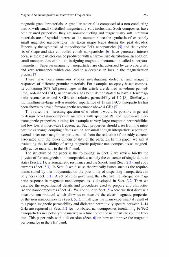
Abstract Most conventional magnetic materials used in the electronic devices areferrites, which are composed of micrometer-size grains. But ferrites have smallsaturation magnetization, therefore the performance at GHz frequencies is ratherpoor. That is why functionalized nanocomposites comprising magnetic nanoparti-cles (e.g. composed of Fe, Co) with dimensions ranging from a few nm to 100 nm,and embedded in dielectric matrices (e.g. silicon oxide, aluminium oxide) have asignificant potential for the electronics industry. When the size of the nanoparticlesis smaller than the critical size for multidomain formation, these nanocompositescan be regarded as an ensemble of particles in single-domain states and the losses(due for example to eddy currents) are expected to be relatively small.

Here we review the theory of magnetism in such materials, and we present anovel measurement method used for the characterization of the electromagneticproperties of composites with nanomagnetic insertions. We also present a few exper-imental results obtained on composites consisting of iron nanoparticles in a dielec-tric matrix.

1 Introduction

For a long time have ferrites been the best choice of material for various applica-tions requiring magnetic response at radio frequencies (RF). In recent times, therehas been a strong demand both from the developers and the end-users side fordecreasing the size of the modern-day portable communication devices and to addnew functionalities that require access to broader communication bands or to otherbands than those commonly used in communication between such devices. All thisshould be achieved without increasing power consumption; rather, a decrease wouldbe desired. The antenna for example is a relatively large component of modern-day communication devices. If the size of the antenna is decreased by a certain

J.V.I. Timonen (B)Molecular Materials, Department of Applied Physics, School of Science and Technology,Aalto University, PO Box 15100, FI-00076 AALTO, Finlande-mail: [email protected]

A. Aldea, V. Bârsan (eds.), Trends in Nanophysics, Engineering Materials,DOI 10.1007/978-3-642-12070-1_11, C! Springer-Verlag Berlin Heidelberg 2010

257

258 J.V.I. Timonen et al.

factor, then the resonance frequency of the antenna is increased by the same factor[1]. As a result, in order to compensate this increase in the resonance frequency,the antenna cavity may be filled with a material in which the wavelength of theexternal radiation field is reduced by the same factor. The wavelength ! inside amaterial of relative dielectric permittivity " and the relative magnetic permeabilityµ is given by ! = !0/

""µ where !0 is the wavelength in vacuum. Hence, it is

possible to decrease the wavelength inside the antenna – and therefore also the sizeof the antenna – by increasing the permittivity or the permeability or the both. Oncethe size reduction is fixed – that is, "µ is fixed – the relative strength between thepermittivity and the permeability needs to be decided. It is known that the balancebetween these two affects the bandwidth of the antenna. Generally speaking, high-"and low-µ materials decrease the bandwidth of the microstrip antenna while low-"and high-µ materials keep the bandwidth unchanged or even increase it [2].

Typical high-µ materials are magnetically soft metals, alloys, and oxides. Ofthese, metals and alloys are unsuitable for high-frequency applications since theyare conducting. On the other hand, non-conducting oxides – such as the ferritesmentioned above – have been used and are still being used in many applications.Their usefulness originates from poor conductivity and the ferrimagnetic ordering.But ferrites are limited by low saturation magnetization which results in a low fer-romagnetic resonance frequency and a cut-off in permeability below the communi-cation frequencies [3]. The ferromagnetic resonance frequency has to be well abovethe designed operation frequency to avoid losses and to have significant magneticresponse. However, modern standards such as the Global System for Mobile com-munications (GSM), the Wireless Local Area Network (WLAN), and the WirelessUniversal Serial Bus (Wireless USB) operate in the Super High Frequency (SHF)band or in its immediate vicinity [4]. The frequency range covered by the SHF bandis 3–30 GHz and it cannot be accessed by the ferrites whose resonance frequency istypically of the order of hundreds of MHz [3]. Hence, other kinds of materials needto be developed for the applications mentioned.

The important issue related to the miniaturization by increasing the permittivityand/or the permeability is the introduced energy dissipation. In some contexts, lossesare good in a sense that they reduce the resonance quality factor and hence increasethe bandwidth. The cost is increased energy consumption which goes to heating ofthe antenna cavity. In general, several processes contribute to losses in magneticmaterials. At low frequencies, the dominant loss process is due to hysteresis: itbecomes less important as the frequency increases, due to the fact that the motion ofthe domain walls becomes dampened. The eddy current loss plays a dominant role inthe higher-frequency range: the power dissipated in this process scales quadraticallywith frequency. In this paper will have a closer look at this source of dissipation,which can be reduced in principle by using nanoparticles instead of bulk materials.Another important process which we will discuss is ferromagnetic resonance (dueto rotation of the magnetization).

All these phenomena limit the applicability of standard materials for high-frequency electronics. However, the SHF band may be accessed by the so called

Magnetic Nanocomposites at Microwave Frequencies 259

magnetic granularmaterials. A granular material is composed of a non-conductingmatrix with small (metallic) magnetically soft inclusions. Such composites haveboth desired properties; they are non-conducting and magnetically soft. Granularmaterials are of special interest at the moment since the synthesis of extremelysmall magnetic nanoparticles has taken major leaps during the past decades.Especially the synthesis of monodisperse FePt nanoparticles [5] and the synthe-sis of shape and size controlled cobalt nanoparticles [6] have generated interestbecause these particles can be produced with a narrow size distribution. In addition,small nanoparticles exhibit an intriguing magnetic phenomenon called superpara-magnetism. Superparamagnetic nanoparticles are characterized by zero coercivityand zero remanence which can lead to a decrease in loss in the magnetizationprocess [7].

There have been numerous studies investigating dielectric and magneticresponses of different granular materials. For example, an epoxy-based compos-ite containing 20% (all percentages in this article are defined as volume per vol-ume) rod-shaped CrO2 nanoparticles has been demonstrated to have a ferromag-netic resonance around 8 GHz and relative permeability of 1.2 [8]. Similarly, amultimillimetre-large self-assembled superlattice of 15 nm FeCo nanoparticles hasbeen shown to have a ferromagnetic resonance above 4 GHz [9].

This raises the interesting question of whether it would be possible in generalto design novel nanocomposite materials with specified RF and microwave elec-tromagnetic properties, aiming for example at very large magnetic permeabilitiesand low loss at microwave frequencies. Such properties should arise from the inter-particle exchange coupling effects which, for small enough interparticle separation,extends over near-neighbour particles, and from the reduction of the eddy currentsassociated with the lower dimensionality of the particles. In this paper, we aim atevaluating the feasibility of using magnetic polymer nanocomposites as magneti-cally active materials in the SHF band.

The structure of the paper is the following: in Sect. 2 we review briefly thephysics of ferromagnetism in nanoparticles, namely the existence of single-domainstates (Sect. 2.1), ferromagnetic resonance and the Snoek limit (Sect. 2.3), and eddycurrents (Sect. 2.3). In Sect. 3 we discuss theoretically issues such as the require-ments stated by thermodynamics on the possibility of dispersing nanoparticles inpolymers (Sect. 3.1). A set of rules governing the effective high-frequency mag-netic response in magnetic nanocomposites is developed in Sect. 3.2. Then wedescribe the experimental details and procedures used to prepare and character-ize the nanocomposites (Sect. 4). We continue to Sect. 5 where we first discuss ameasurement protocol which allow us to measure the electromagnetic propertiesof the iron nanocomposites (Sect. 5.1). Finally, as the main experimental result ofthis paper, magnetic permeability and dielectric permittivity spectra between 1–14GHz are reported in Sect. 5.2 for iron-based nanocomposites (containing Fe/FeOnanoparticles in a polystyrene matrix) as a function of the nanoparticle volume frac-tion. This paper ends with a discussion (Sect. 6) on how to improve the magneticperformance in the SHF band.


2 Magnetism in Nanoparticles

Magnetic behavior in ferromagnetic nanoparticles is briefly reviewed in this sec-tion c.f. [10–12]. The focus is especially in the so called single-domain magneticnanoparticles which lack the typical multi-domain structure observed in bulk ferro-magnetic materials. The topics to be discussed are: (A) when does the single-domainstate appear, (B) what is its ferromagnetic resonance frequency, and (C) what are thesources of energy dissipation in single-domain nanoparticles.

2.1 Existence Criteria for the Single-Domain State

A magnetic domain is a uniformly magnetized region within a piece of ferro-magnetic or ferrimagnetic material. Magnetic domains are separated by boundaryregions called the domain walls (DW) in which the magnetization gradually rotatesfrom the direction defined by one of the domains to the direction defined by theother. The domain wall thickness (dDW), which depends on the material’s exchangestiffness coefficient (A) and the anisotropy energy density (K ), extends from 10 nmin high-anisotropy materials to 200 nm in low-anisotropy materials. The domainthickness, on the other hand, depends more on geometrical considerations. Forexample, in one square centimeter iron ribbon, 10 µm thick, the domain wall spac-ing is of the order of 100 µm. The spacing increases if the thickness is reduced.Reducing the thickness over a critical value leads to the complete disappearance ofthe domain walls. That state is called the single-domain (SD) state. Between mul-tidomain and single-domain states there may be a vortex state: this is not discussedhowever here. Similarly, the domains in spherical nanoparticles vanish below a cer-tain diameter which is of the order of few nanometers or few tens of nanometers.In hard materials this diameter (dSD,HARD) can be estimated to be roughly ([11],p. 303):

dSD,HARD # 18

"AK

µ0 M2S

, (1)

where MS is the saturation magnetization and µ0 is the vacuum permeability. Theequation is based on the assumption that the magnetization follows the energeticallyfavorable directions (easy axes or easy planes) defined by the anisotropy. The single-domain diameter given by Eq. (1) should be always compared to the domain wallthickness given by ([11], p. 283)

dDW = #

!AK

. (2)

If the diameter of the particle is less than the wall thickness, it is obvious that itcannot support the wall. The condition dSD,HARD > dDW, leads to the criterion


Q def= 18#

K

µ0 M2S

> 1. (3)

On the other hand, in magnetically soft nanoparticles the magnetization does notnecessary follow the easy directions. In the perfectly isotropic case, that is K = 0,the surface spins are oriented along the spherical surface and a vortex core is formedin the center of the particle if the particle is above the single-domain limit. Thesingle-domain diameter (dSD,SOFT) of a perfectly isotropic nanoparticle is given by([11], p. 305),

dSD,SOFT # 6

"A

µ0 M2S

#ln

dSD,SOFT

a$ 1

$, (4)

where a is the lattice constant. This equation can be solved by the iteration method.The single-domain diameter is more difficult to estimate if the anisotropy is non-zero but does not meet the requirement of Eq. (3). In that case, the single-domaindiameter is likely to rest between the values predicted by Eqs. (1) and (4).

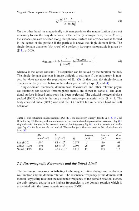
Single-domain diameters, domain wall thicknesses and other relevant physi-cal quantities for selected ferromagnetic metals are shown in Table 1. The addi-tional surface-induced anisotropy has been neglected. The uniaxial hexagonal closepacked (HCP) cobalt is the only strongly anisotropic material with Q # 1. Thebody centered cubic (BCC) iron and the FCC nickel fall in between hard and softbehavior.

Table 1 The saturation magnetization (MS) [13], the anisotropy energy density K [13, 14], theQ-factor Eq. (3), the single-domain diameter in the hard material approximation dSD,HARD Eq. (1),single-domain diameter in the isotropic material limit dSD,SOFT Eq. (4), and the domain wall widthdDW Eq. (2), for iron, cobalt, and nickel. The exchange stiffnesses used in the calculations arefrom [15]

MS K dSD,HARD dSD,SOFT dDW(emu/cm3) (erg/cm3) Q (nm) (nm) (nm)

Iron (BCC) 1707 4.8 % 105 0.075 5 89 63Cobalt (HCP) 1440 4.5 % 106 0.996 26 169 26Nickel (FCC) 485 $5.7 % 104 0.110 13 173 113

2.2 Ferromagnetic Resonance and the Snoek Limit

The two major processes contributing to the magnetization change are the domainwall motion and the domain rotation. The resonance frequency of the domain wallmotion is typically less than the resonance frequency of the domain rotation. Hence,the only process active in the highest frequencies is the domain rotation which isassociated with the ferromagnetic resonance (FMR).


The natural1 ferromagnetic resonance was first explained by Snoek to be theresonance of the magnetization vector ( &M) pivoting under the action of some energyanisotropy field ( &HA) [16]. The origin of the anisotropy is not restricted. It can beinduced, for example, by an external magnetic field, magnetocrystalline anisotropyor shape anisotropy. It is common to treat any energy anisotropy as if it was due toan external magnetic field.

The motion of the magnetization around in the anisotropy field is described bythe Landau-Lifshitz equation [17],

d &Mdt

= $$( &M % &HA) $ 4#µ0!̂

M2S

( &M % ( &M % &HA)), (5)

where !̂ is the relaxation frequency (not the resonance frequency) and $ is the gyro-magnetic constant given by ([10], p. 559)

$ = geµ0

2m# 1.105 % 105g(mA$1s$1) # 2.2 % 105mA$1s$1, (6)

where g is the gyromagnetic factor (taken to be 2), e is the magnitude of the electroncharge and m is the electron mass.

If the Landau-Lifshitz equation is solved, one obtains the resonance condition([10] p. 559)

fFMR = (2#)$1$HA, (7)

where fFMR is the resonance frequency and HA is the magnitude of the anisotropyfield.

For example, for HCP cobalt the magnetocrystalline anisotropy energy density(UA) is given by ([10], p. 264)

UA = K sin2% # K%

%2 $ 13%4 + . . .

&, (8)

1“Natural” is used so that this resonance is distinguished from the dimensional resonance asso-ciated with standing waves within a sample of finite size. The dimensional resonance takesplace when the end-to-end length (L) of the sample times two is equal to an integer multipleof the wavelength of the radiation (!) in the material. The same is mathematically expressed asL = n!/2 = n/2!0/

""µ where !0 is the wavelength in vacuum and n is a positive integer. The

resonance frequency ( fr ) is given by fr = c/!0 = nc/2L"

"µ where c is the speed of light. Forexample, the first dimensional resonance in a 10 mm long sample with "µ = 9 is approximately5 GHz. The dimensional resonance can be avoided in experiments by carefully estimating theproduct "µ and designing the sample length accordingly.


where % is the angle between the easy axis and the magnetization. The energy den-sity due to an imaginary magnetic field is given by ([10], p. 264)

UA = $µ0 HA MScos % # $µ0 HA MS

%1 $ 1

2%2 + . . .

&. (9)

By comparing the exponents one obtains

HA = 2Kµ0 MS

# 0.62 Tµ0

, (10)

and from Eq. (7)

fFMR = (2#)$1$HA # 17 GHz. (11)

It is tempting to use nanoparticles with as high anisotropy as possible in order tomaximize the FMR frequency. Unfortunately, the permeability decreases with theincreasing anisotropy; for uniaxial materials the relative permeability µ is given by([10], p. 493),

µ = 1 + µ0 M2Ssin2%

2K. (12)

It is easy to show that that Eqs. (7),(10), and (12) lead to

'µ( · fFMR = $MS

3#, (13)

where 'µ( is the angular average of the relative permeability (which we assumemuch larger than the unit). This equation is known as the Snoek limit. It is anextremely important result since it predicts the maximum permeability achievablewith a given FMR frequency as a function of the saturation magnetization. It can beshown to be valid for both the uniaxial and cubic materials (taken that K > 0). Somevalues for the maximum relative permeability as a function of the FMR frequencyand the saturation magnetization are shown in Table 2.

It has been found out that the Snoek limit can be exceeded in materials of negativeuniaxial anisotropy [18]. In that case, the magnetization can rotate in the easy planeperpendicular to the c-axis. Such materials obey the modified Snoek limit ([10],p. 561)

µ · fFMR = $MS

3#

"HA1

HA2, (14)

where HA1 is the anisotropy field along the c-plane (small) and HA2 is the anisotropyfield out of the c-plane (large). One such material is the Ferroxplana [12].


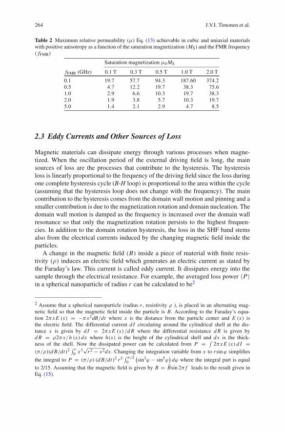
Table 2 Maximum relative permeability (µ) Eq. (13) achievable in cubic and uniaxial materialswith positive anisotropy as a function of the saturation magnetization (MS) and the FMR frequency( fFMR)

Saturation magnetization µ0 MS

fFMR (GHz) 0.1 T 0.3 T 0.5 T 1.0 T 2.0 T

0.1 19.7 57.7 94.3 187.60 374.20.5 4.7 12.2 19.7 38.3 75.61.0 2.9 6.6 10.3 19.7 38.32.0 1.9 3.8 5.7 10.3 19.75.0 1.4 2.1 2.9 4.7 8.5

2.3 Eddy Currents and Other Sources of Loss

Magnetic materials can dissipate energy through various processes when magne-tized. When the oscillation period of the external driving field is long, the mainsources of loss are the processes that contribute to the hysteresis. The hysteresisloss is linearly proportional to the frequency of the driving field since the loss duringone complete hysteresis cycle (B-H loop) is proportional to the area within the cycle(assuming that the hysteresis loop does not change with the frequency). The maincontribution to the hysteresis comes from the domain wall motion and pinning and asmaller contribution is due to the magnetization rotation and domain nucleation. Thedomain wall motion is damped as the frequency is increased over the domain wallresonance so that only the magnetization rotation persists to the highest frequen-cies. In addition to the domain rotation hysteresis, the loss in the SHF band stemsalso from the electrical currents induced by the changing magnetic field inside theparticles.

A change in the magnetic field (B) inside a piece of material with finite resis-tivity (&) induces an electric field which generates an electric current as stated bythe Faraday’s law. This current is called eddy current. It dissipates energy into thesample through the electrical resistance. For example, the averaged loss power 'P(in a spherical nanoparticle of radius r can be calculated to be2

2 Assume that a spherical nanoparticle (radius r , resistivity & ), is placed in an alternating mag-netic field so that the magnetic field inside the particle is B. According to the Faraday’s equa-tion 2#x E (x) = $#x2dB/dt where x is the distance from the particle center and E (x) isthe electric field. The differential current d I circulating around the cylindrical shell at the dis-tance x is given by d I = 2#x E (x) /d R where the differential resistance d R is given byd R = &2#x/h (x) dx where h(x) is the height of the cylindrical shell and dx is the thick-ness of the shell. Now the dissipated power can be calculated from P =

'2#x E (x) d I =

(#/&)(d B/dt)2 ' r0 x3

"r2 $ x2dx . Changing the integration variable from x to rsin ' simplifies

the integral to P = (#/&) (d B/dt)2 r5 ' #/20

(sin3' $ sin5'

)d' where the integral part is equal

to 2/15. Assuming that the magnetic field is given by B = B̂sin 2# f leads to the result given inEq. (15).


'P( = 2#

151&

r5

*%d Bdt

&2+

= 4#3

15&r5

,f B̂

-2, (15)

where f is the frequency of the driving field and B̂ is the amplitude of the oscil-lating component of the total magnetization. From Eq. (15) it is obvious that theloss power per unit volume increases as r2, indicating that the loss can be decreasedby using finer nanoparticles. Notice that the loss power will vanish above the FMRresonance since there cannot be magnetic response above that frequency, that isB̂ ) 0.

For example, the loss power per unit volume (p) in cobalt nanoparticles can becalculated to be

p # 32, r

nm

-2%

fGHz

&2.

B̂T

/2W

cm3 . (16)

If the volume of the magnetic element is 0.1 cm3, the radius of the nanoparticles5 nm, and B̂ = 1.8 T one obtains 0.26 mW for loss power.

It has been shown that this simple approach is inadequate to describe the eddycurrent loss in materials containing domain walls [10]. The eddy currents in mul-tidomain materials are localized at the domain walls, which leads to a roughlyfour-times increase in the loss. However, since there are no walls present in single-domain nanoparticles and the magnetization reversal can take place by uniform rota-tion, this model is considered here to be adequate in describing the eddy current lossin single-domain nanoparticles.

One more matter to be addressed is the penetration depth of the magnetic fieldinto the nanoparticles. Because the eddy currents create a magnetic field counter-acting the magnetic field that induced the eddy currents, the total magnetic field isreduced when moving from the nanoparticle surface towards its core. The depth (s)at which the magnetic field is reduced by the factor 1/e is called the skin-depth andit is given by ([10], p. 552),

s ="

2&

(µµ0. (17)

For example, from Eq. (17) the skin-depth for cobalt (& = 62 n)m and µ= 10) at1 GHz is 1.3 µm and at 10 GHz 400 nm. Hence, cobalt nanoparticles that are lessthan 100 nm in diameter would already be on the safe side. The situation is ratherdifferent in typical ferrites for which & # 104 )m and µ=103, giving 5 cm forthe skin depth. Therefore ferrites can be used in the bulk form in near-microwaveapplications.


3 Magnetic Polymer Nanocomposites

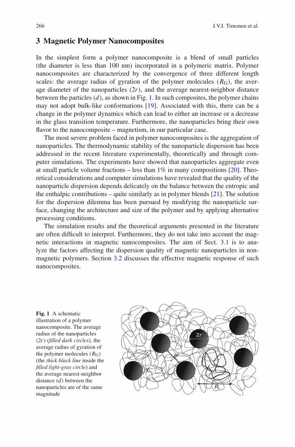
In the simplest form a polymer nanocomposite is a blend of small particles(the diameter is less than 100 nm) incorporated in a polymeric matrix. Polymernanocomposites are characterized by the convergence of three different lengthscales: the average radius of gyration of the polymer molecules (RG), the aver-age diameter of the nanoparticles (2r), and the average nearest-neighbor distancebetween the particles (d), as shown in Fig. 1. In such composites, the polymer chainsmay not adopt bulk-like conformations [19]. Associated with this, there can be achange in the polymer dynamics which can lead to either an increase or a decreasein the glass transition temperature. Furthermore, the nanoparticles bring their ownflavor to the nanocomposite – magnetism, in our particular case.

The most severe problem faced in polymer nanocomposites is the aggregation ofnanoparticles. The thermodynamic stability of the nanoparticle dispersion has beenaddressed in the recent literature experimentally, theoretically and through com-puter simulations. The experiments have showed that nanoparticles aggregate evenat small particle volume fractions – less than 1% in many compositions [20]. Theo-retical considerations and computer simulations have revealed that the quality of thenanoparticle dispersion depends delicately on the balance between the entropic andthe enthalpic contributions – quite similarly as in polymer blends [21]. The solutionfor the dispersion dilemma has been pursued by modifying the nanoparticle sur-face, changing the architecture and size of the polymer and by applying alternativeprocessing conditions.

The simulation results and the theoretical arguments presented in the literatureare often difficult to interpret. Furthermore, they do not take into account the mag-netic interactions in magnetic nanocomposites. The aim of Sect. 3.1 is to ana-lyze the factors affecting the dispersion quality of magnetic nanoparticles in non-magnetic polymers. Section 3.2 discusses the effective magnetic response of suchnanocomposites.

Fig. 1 A schematicillustration of a polymernanocomposite. The averageradius of the nanoparticles(2r) (filled dark circles), theaverage radius of gyration ofthe polymer molecules (RG)(the thick black line inside thefilled light-gray circle) andthe average nearest-neighbordistance (d) between thenanoparticles are of the samemagnitude

d

2r

RG


3.1 Factors Affecting the Nanoparticle Dispersion Quality

3.1.1 Attractive Interparticle Interactions

There has been considerable interest in modifying chemically the nanoparticle sur-face towards being more compatible with the polymer [22, 23]. Especially importantsurface modification techniques are the grafting-techniques. They involve either asynthesis of polymer molecules onto nanoparticle surface (grafting-from) or attach-ment of functionalized polymers onto the the nanoparticle surface (grafting-to). Theadvantage of the grafting-techniques is that they can make the nanoparticle surfacenot only enthalpically compatible with a polymer, but the grafted chains also exhibitsimilar entropic behavior as the surrounding polymer molecules. One disadvantageis that these techniques require precise knowledge of the chemistry involved.

It is well-established that a monolayer of small molecules attached to thenanoparticle surface is not enough to significantly enhance the quality of the dis-persion even if the surface molecules were perfectly compatible with the polymer –that is, they were identical to the constitutional units of the polymer. This is dueto the fact that the London dispersion force3 acting between the nanoparticles iseffective over a length which increases linearly with the nanoparticle diameter. Thisis proven in the following.

The London dispersion energy (ULONDON) between two identical spheres, diam-eters 2r , separated by a distance d was first shown by Hamaker to be [24],

ULONDON = $ A121

6

0(2r)2

2(2r + d)2 + (2r)2

2((2r + d)2 $ (2r)2)

+ ln

.

1 $ (2r)2

(2r + d)2

/ 1

, (18)

where A121 is the effective Hamaker for the nanoparticles (phase 1) immersed inthe polymeric matrix (phase 2). The Hamaker constants are typically listed for twoobjects of the same material in vacuum from which the effective value can be cal-culated by using the approximation [24]

A121 #,2

A11 $2

A22

-2, (19)

where A11 is the Hamaker constant for the nanoparticles and A22 is the Hamakerconstant for the medium. The typical effective Hamaker constant for metal particlesimmersed in organic solvent or a polymer is approximately 25·10$20 J. By using thisvalue, the London potential Eq. (18) is plotted for 5 nm metal particles in Fig. 2a andfor 15 nm particles in Fig. 2b. The distance

(dkBT ,LONDON

)over which the London

3Despite of its name it is an attractive force.


0 5 10–10

–8

–6

–4

–2

0

d (nm) d (nm)

U (

k B T

)

U (

k B T

)

0 10 20 30 40 50–50

–40

–30

–20

–10

0

0 5 10 150

10

20

30

2r (nm)

d kB T

(nm

)BA

DC

d

2r

Fig. 2 Comparison between the London dispersion force and the magnetic dipolar interactionbetween two identical metal nanoparticles. (a) The reduced London potential Eq. (18) (grey thincurve), the magnetic dipolar energy Eq. (24) (black thin curve) and the total interaction energy(black thick curve) between two 5 nm metal nanoparticles. (b) The same for two metal particles15 nm in diameter. The magnetic dipolar energy curve is overlapping with the total interactioncurve. (c) The distance between the particle surfaces as a function of the particle diameter when theinteraction energy is comparable to the thermal energy. The black line corresponds to the magneticinteraction Eq. (25) and the grey to the London dispersion Eq. (20). (d) Schematic illustration anddefinition of the used variables

dispersion force is effective can be estimated by setting the interaction energy equalto the thermal energy and by solving for the distance. The result is4

dkBT ,LONDON = (* $ 1) · 2r # 2r3

, (20)

where * is a constant in excess of unity and typically around 1.33 for metalsimmersed in organic medium. This linear dependence is shown in Fig. 2c. Typically,

4By setting ULONDON = $kBT and defining a reduced variable * = 1 + dkBT,LONDON/2r onecan rewrite Eq. (18) as 6kBT/A121 = 1/(2*2) + 1/[2

(*2 $ 1

)] + ln

(1 $ 1/*2) * f (*) . This

equation can be solved for * by plotting y = f (*) and y = 6kBT/A121 and by locating the pointof intersection. The effective distance can be calculated by inserting the obtained intersection pointinto the equation defining the reduced variable.


nanoparticles are covered with a monolayer of alkyl chains ranging up to 20 carbon-carbon bonds in length. Even if the chains were totally extended and rigid, theirlength would be only roughly 2 nm. Such a shielding layer can protect only nanopar-ticles less than 12 nm in diameter from aggregation.

Fortunately, the thermodynamic equilibrium is not solely dependent on theenthalpy which always drives the system towards the phase separation. The addi-tional component is entropy which opposes the separation. The Gibbs free energy(G) which determines the thermodynamic stability in the constant temperature andthe constant pressure is given by G = H $T S, where H is enthalpy and S is entropy.The entropic term per unit volume in a mixture of nanoparticles and small molecularweight solvent molecules can be estimated to be5

$ T SV

= $kBTVS

#ln

%x

x $ +

&+ +

xln

%x $ +

+

& $# $kBT

VS

+

xln

x+

, (21)

where VS is the volume of the solvent molecule, + is the volume fraction ofthe nanoparticles and x is the volume ratio between a nanoparticle and a solventmolecule. In the case of x = 1 the equation properly reduces to

$ T SV

= $kBTVS

[$+ln + $ (1 $ +) ln (1 $ +)] , (22)

which corresponds to the entropy of mixing between two molecules of the samesize.

For example, the volume of a toluene molecule is approximately 0.177 nm3 andthe volume of a 10 nm nanoparticle is 524 nm3. In that case x # 3000. Equa-tion (21) states that the entropy of mixing is reduced by a factor 1/1300 in a 1%nanocomposite when compared to a situation in which both the nanoparticles andthe solvent molecules were of the same size. Without a proof, it is suggested thatthe magnitude of the entropy is even less when the nanoparticles are mixed withpolymer molecules. The suggestion is justifiable due to the entropic restrictionsintroduced by covalent bonding between the monomer units.

If the nanoparticles are magnetic, they interact with each other more strongly thannon-magnetic nanoparticles. The magnetic dipolar interaction energy (UM) betweentwo particles, 2r in diameter, is given by [10]

UM = µ0

4#(d + 2r)3 (3 (m1 ·3r ) (m2 · 3r ) $ m1 · m2) , (23)

5Assume that an arbitrary lattice of N sites is filled with N1 nanoparticles and N2 solvent molecules.Each nanoparticle incorporates x lattice sites and each solvent molecule one lattice site. Then thenumber of microstates ()) is approximately ) # N !/((N $ N1)!N1!). Notice that N $ N1 += N2in contrast to the mixing theory of small molecules of same size. The Eq. (22) is obtained fromthe definition of entropy S = kBln ) by simple algebraic manipulation and by assuming that thedensity of the nanoparticles is low (N1 , N ).


where3r is the unit vector between the particles, d is the distance between the particlesurfaces and m1 and m2 are the magnetic moments of the particles. Assuming thatthe particles are magnetically single-domain, their saturation magnetization is MSand that the magnetization vectors are parallel to each other and to the unit vector,the interaction energy is reduced to

UM = $8#

9r6

(d + 2r)3 µ0 M2S . (24)

Similarly to the effective distance of the London dispersion force, one can derivethe distance at which the magnetic energy is comparable to the thermal energy. It isgiven by

dkBT,MAGNETIC =.

8#

9µ0 M2

S

kBT

/ 13

r2 $ 2r. (25)

To give an example, the magnetic interaction energy Eq. (24) is drawn for twopairs of cobalt particles, 5 nm and 15 nm in diameter, in Fig. 2a and b, respectively.The interaction between the 5 nm particles is dominated by the London dispersionpotential and only weakly modified by the magnetic interaction. In the case of the15 nm particles, the magnetic interaction is effective over a distance of 50 nm, ren-dering the London attraction negligible. In order to shield magnetic nanoparticlesfrom such a long-ranging interaction with a protective shell is unpractical. First ofall, the maximum achievable nanoparticle volume fraction

,+̂MAGNETIC

-is lim-

ited by the shielding. If the shielding layer volume is not taken to be a part of thenanoparticle volume, the maximum achievable volume fraction (neglecting entropicconsiderations) is proportional to

+̂MAGNETIC - r3

(dkBT,MAGNETIC + 2r

)3 - r$3. (26)

On the other hand, the maximum volume fraction,+̂LONDON

-limited by shielding

against the London attraction does not depend on the nanoparticle size:

+̂LONDON - r3

(dkBT,LONDON + 2r

)3 = const. (27)

Second, the shielding against the magnetic dipolar attraction by using the conven-tional grafting techniques is difficult due to the enormous length required from thegrafted chains.

Based on the considerations presented in this section, it is unlikely that a uni-form dispersion of magnetic nanoparticles of decent size can be achieved by usingthe conventional shielding strategy. The magnetic interaction starts to dominate the


free energy when the magnetic nanoparticles are 10 nm in diameter or larger. Fur-thermore, the entropic contribution decreases approximately as x$1 where x is thevolume of the nanoparticle relative to the volume of the solvent molecule. Hence,the dispersion dilemma needs to be approached from some other point of view thanthe conventional shielding strategy.

3.1.2 Effect of the Polymer Size, Architecture, and Functionalization

A general dispersion strategy proposed by Mackay et al. suggests that the qualityof a nanoparticle dispersion is strongly enhanced if the radius of gyration of thepolymer is larger than the average diameter of the nanoparticle [20]. The radius ofgyration (RG) for a polymer molecule which is interacting neutrally with its sur-roundings is given by RG # "

C/6"

Na where N is the number of monomers, ais the length of a single monomer and C is the Flory ratio. For the polystyrene thatfor example we use the equation yields 16 nm for the radius of gyration (C # 9.9,N # 2400 and a # 0.25 nm). It is based on the assumption that small particlescan be incorporated within polymer chains easily but large particles prevent chainsfrom achieving their true bulk conformations. In other words, large particles stretchthe polymer molecules and hence introduce an entropic penalty. Pomposo et al.have verified the Mackay’s proposition in a material consisting of polystyrene andcrosslinked polystyrene nanoparticles [25]. Such a system is ideal in a sense thatthe interaction between the polymer matrix and the nanoparticles is approximatelyneutral. That emphasizes the entropic contribution to the free energy. However, if themain contribution to the free energy is enthalpic, as it is in magnetic nanocompos-ites, one should use the Mackay’s proposition with a considerable care. The entropicenhancement is most likely much smaller than the enthalpic term, rendering theimprovement in the dispersion quality negligible.

One other remedy for the dispersion dilemma is to replace the linear polymer bya star-shaped one. It has been shown both theoretically [21] and experimentally [26]that it can lead to a spontaneous exfoliation of a polymer-nanoclay composite. It hasbeen also demonstrated that replacing polystyrene in a polystyrene-nanoclay com-posite by a telechelic hydroxyl-terminated polystyrene results in exfoliation. Sincethe polymer-nanoclay composites are geometrically different from the polymer-nanoparticle composites, one cannot directly state that these techniques would alsowork with polymer-nanoparticles composites.

3.2 Effective Magnetic Response

The effective relative permeability of a nanocomposite containing spherical mag-netic inclusions can be determined from several different effective medium theories(EMT) [27]. The two most popular are the Maxwell-Garnett formula

µ = 1 + 3+µNP$1

µNP + 2 $ + (µNP $ 1), (28)


10

9

8

7

6

5

4

3

2

10 0.2 0.4

Effe

ctiv

e pe

rmea

bilit

y µ

0.6Nanopracticle volume fraction !

0.8 1

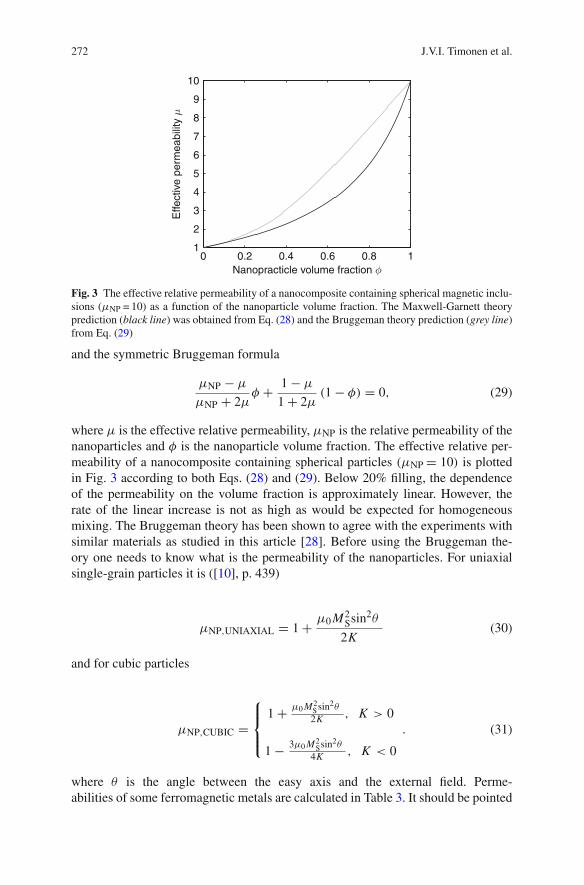
Fig. 3 The effective relative permeability of a nanocomposite containing spherical magnetic inclu-sions (µNP = 10) as a function of the nanoparticle volume fraction. The Maxwell-Garnett theoryprediction (black line) was obtained from Eq. (28) and the Bruggeman theory prediction (grey line)from Eq. (29)

and the symmetric Bruggeman formula

µNP $ µ

µNP + 2µ+ + 1 $ µ

1 + 2µ(1 $ +) = 0, (29)

where µ is the effective relative permeability, µNP is the relative permeability of thenanoparticles and + is the nanoparticle volume fraction. The effective relative per-meability of a nanocomposite containing spherical particles (µNP = 10) is plottedin Fig. 3 according to both Eqs. (28) and (29). Below 20% filling, the dependenceof the permeability on the volume fraction is approximately linear. However, therate of the linear increase is not as high as would be expected for homogeneousmixing. The Bruggeman theory has been shown to agree with the experiments withsimilar materials as studied in this article [28]. Before using the Bruggeman the-ory one needs to know what is the permeability of the nanoparticles. For uniaxialsingle-grain particles it is ([10], p. 439)

µNP,UNIAXIAL = 1 + µ0 M2Ssin2%

2K(30)

and for cubic particles

µNP,CUBIC =

456

57

1 + µ0 M2Ssin2%

2K , K > 0

1 $ 3µ0 M2Ssin2%

4K , K < 0

. (31)

where % is the angle between the easy axis and the external field. Perme-abilities of some ferromagnetic metals are calculated in Table 3. It should be pointed


Table 3 The saturation magnetization MS [13], the anisotropy energy density (K) [13, 14], andthe calculated relative permeabilities µNP (from Eqs. (30) and (31)) for selected ferromagneticmetals. 'µNP( refers to the calculation where the permeability has been averaged over the isotropicdistribution of the easy axes

MS K µNP(emu/cm3) (erg/cm3) (% = #/2) 'µNP(

Iron (BCC) 1707 4.8 % 105 39 26Cobalt (HCP) 1440 4.5 % 106 4 3Nickel (FCC) 485 $5.7 % 104 40 27

out that once again the surface anisotropy has been neglected, and that it is mostlikely that the experimentally determined permeabilities are smaller than those inTable 3.

The effective magnetic response of a polymer nanocomposite containing single-domain nanoparticles can be determined from the following rules:

• The FMR frequency determines the high-frequency limit of the magneticresponse. The FMR frequency is determined from the effective anisotropy fieldby using Eq. (7).

• The permeability below the FMR is dispersion-free since the only magnetizationprocess taking place in single-domain particles is the domain rotation (which isassociated with the FMR).

• The magnitude of the permeability is determined from the Bruggeman theory,Eq. (29).

• The permeability of the nanoparticles – which is used in the Bruggemantheory – is determined from the effective anisotropy energy density and the satu-ration magnetization according to the Eqs. (30) and (31).

The anisotropy used in the calculations should be the true total anisotropy:the sum of the (bulk) magnetocrystalline anisotropy, the surface anisotropy,and the anisotropy due to magnetic field. Especially if the bulk anisotropy issmall, the surface anisotropy can be the dominant term. Since the experimentaldata on the surface anisotropy is scarce, it has been neglected in the analysisso far.

4 Preparation and Characterization

In this section we describe the experimental details and procedures used to prepareand characterize the nanocomposites.

4.1 High Volume Fraction Nanocomposites for High-Frequencies

Nanocomposites containing iron nanoparticles for the SHF band characteriza-tion were made according to the following procedure. First, a desired amount of


Table 4 Compositions of the nanocomposites prepared for electromagnetic characterization

Designation Nanoparticle type ' (%)

PS/QS-Fe 5% Quantum sphere iron 5PS/QS-Fe 10% Quantum sphere iron 10PS/QS-Fe 15% Quantum sphere iron 14.7

nanoparticles (provided by Quantum Sphere, from now on abbreviated QS) wereweighted and mixed with 15 ml of toluene (Fluka, purity better than 99.7%). Thedesired amount of polystyrene was added and allowed to dissolve before vigurouslysonicating the solution to break nanoparticle aggregates. The toluene was allowedto evaporate, resulting in a dark polystyrene-like film which was then collected.

Using this method, we have prepared nanocomposites of iron nanoparticles, withthree different concentrations, 5, 10 and 15% (see Table 4).

4.2 Transmission Electron Microscopy: Structural Analysis

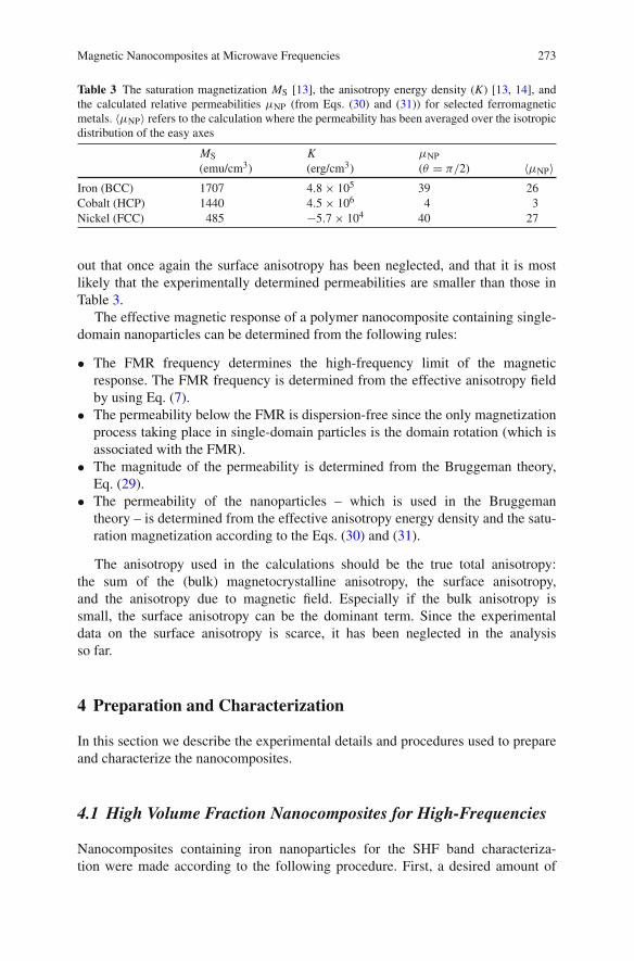
The nanoparticles were imaged with a TEM (FEI Company model Tecnai G2BioTwin) in bright field at the acceleration voltage of 120 kV. Before imaging thealignment of the microscope was checked and corrected. The image was recordedwith a digital camera (Gatan model UltrascanTM 1000) and its contrast and bright-ness was adjusted after acquisition. An image of iron nanoparticles is shown inFig. 4.

Fig. 4 Bright field TEM images of the quantum sphere iron (scale bar is 50 nm)


4.3 Magnetometry: Low-Frequency Permeability

Static hysteresis loops (the magnetization versus the applied field) of the nanoparti-cles were measured with a Superconducting Quantum Interference Device (SQUID)magnetometer (Quantum Design model MPMS XL) at 300 K. Roughly 1 mg of thenanoparticles was encapsulated in a piece of aluminum foil (approximately 100 mg)and attached to the plastic straw sample holder with Kapton tape. The permeabilitywas extracted from the measured magnetization curve by fitting a straight line tothe low-field part of the curve. The demagnetizing factor was approximated to bezero because the nanoparticles were compressed into flat layers inside the aluminumwrap and the layer surface was aligned along the external field.

4.4 X-Ray Diffraction: Structure of the Nanoparticles

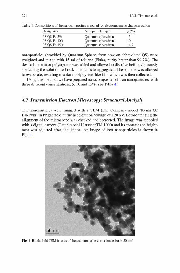
The nanoparticle structure was analyzed with XRD. The diffraction intensities of thenanoparticles were measured as a function of the diffraction angle 2% with a diffrac-tometer (PANalytical model X’Pert PRO MRD) using Cu K* radiation (wavelengthof 0.154056 nm) at room temperature. The XRD patterns of QS-Fe nanoparticlesis shown in Fig. 5. The samples were prepared by filling a circular cavity (35 mmin diameter and 0.7 mm high) bored into an acrylic glass plate with the particles.The powder was compressed and smoothed with a piece of a silicon wafer. Theadhesion between the powder and the plate was sufficient to hold the powder withinthe cavity even though the plate was turned vertically for the measurement. Thesample was scanned from 30. to 90. for one hour. The resulting data was processedby first stripping off the peaks due to the Cu K*2 radiation and by filtering thebackground noise. The data was smoothed if the signal-to-noise ratio was poor.Second, the Lorentzian function was fitted to all peaks using the (self-implemented)Gauss-Newton algorithm. The performance of the algorithm was excellent in thecase of well-defined peaks, but vague peaks had to be fitted manually. From the fittedpeaks the angle, the FWHM and the intensity (integrated over the peak area) wereextracted. Based on these values, the composition of nanoparticles was determined.Furthermore, the coherently scattering domain size was estimated from broadeningof the FWHM. The natural width of a peak due to diffractometer was determinedby measuring an annealed silicon powder sample and assuming that the coherently

30 40 50 60 70 80 90100

101

102

2!

Intensity QS!Fe

Fig. 5 XRD spectrum of iron nanoparticles


scattering domains were so large that their contribution to the broadening of theFWHM was negligible. The broadening due to the lattice strain was assumed to beminimal.

4.5 Summary

To summarize our results (see Table 5), we find that The Quantum Sphere iron(QS-Fe) nanoparticles are roughly 20–30 nm in diameter and most of the particlesexhibit a core-shell structure. Based on the XRD analysis, the core is suggested tocomprise 9 nm BCC iron crystallites and the shell 3 nm FeO crystallites. The com-position was determined to be a 50–50% balance between the oxide and the metalphases. The measured saturation magnetization (125 emu/g) is in rough agreementwith the metal volume fraction estimated from XRD and the saturation magnetiza-tion given in literature for pure iron (218 emu/g) [13].

Table 5 Summary of the nanoparticles and their properties. Particle diameters d were estimatedfrom the TEM images and the crystalline composition and the average crystallite diameters dCRYSTfrom the XRD measurement

MS Crystal dcrystd nm (emu/g) µ (nm) ' (%) (nm)

Quantum sphere iron 20–30 125 12.3 Fe (BCC) 50 ± 5 9 ± 1FeO 50 ± 5 3 ± 1

5 High-Frequency Properties

5.1 Coaxial Airline Technique: Permittivity and Permeabilityin the SHF Band

A broadband coaxial airline method developed in [29] was used to measure thecomplex permittivity and the complex permeability of magnetic composites inthe superhigh-frequency band (SHF). The technique involves measurement of thereflection parameters S11 and S22, the transmission parameters S12 and S21, and thegroup delay through a sample inserted inside a 7 mm precision coaxial airline. Themeasurement was done by connecting the coaxial airline to a vector network ana-lyzer (Rohde and Schwarz ZVA40) using a pair of high-performance cables (Anritsu3671K50-1). Prior to the measurement, the errors due to the loss and reflection in thecables, connectors and the network analyzer were removed by performing a SOLTcalibration up to both ends of the RF cables.

The sample required in the coaxial waveguide measurement is a cylinder, 7.00mm in diameter, with a 3.04 mm hole in the middle. Its thickness can be adjustedbetween 4 and 10 mm in order to avoid the dimensional resonance. The sam-ples were made by hot-pressing each nanocomposite inside a polished 7 mm hole


drilled through a steel plate. Prior to the pressing, the plate and the nanocompositesinside the holes were sandwiched between two sheets of poly(ethylene terephtha-late) and further between two solid steel plates. The assembly was inserted into ahot-press (Fontijne model TP 400) at 160.C and kept there for two minutes. Afterthe nanocomposite had softened, a 400 kN force was applied over the plates. Afterwaiting for another two minutes, the pressure was released and the plate systemwas disassembled. The holes containing the softened and compressed nanocompos-ites were refilled and the pressing was done again. The filling was repeated onemore time. After the third pressing, the assembly was placed between two metalplates cooled with circulating water under a 400 kN force. After the plates hadcooled down to room temperature, the pressure was released and the plates weredisassembled. Before detaching the solidified cylindrical samples, the plate withthe samples was sandwiched between two 5 mm thick steel plates with 3.1 mmholes exactly above and under of each of the 7 mm holes in the central plate.All the three plates were aligned with respect to each other and clamped together.The assembly was fixed under a vertical boring machine and holes were drilledthrough the nanocomposites through the guiding 3.10 mm holes in the upper plate.The used drill bit was 2.9 mm in diameter since it was found out that the drillingproduced holes 0.1–0.2 mm wider than the drill bit. After drilling, the construc-tion was disassembled and the samples were detached by gently pushing themout of the holes. If necessary, the pellets were finished by carefully removingany imperfections with sandpaper. The sample dimensions were measured with acaliper.

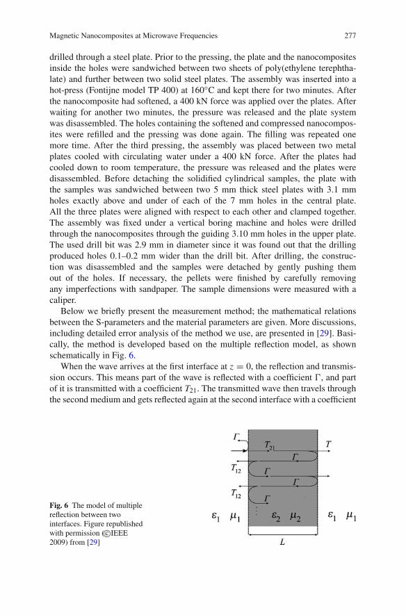
Below we briefly present the measurement method; the mathematical relationsbetween the S-parameters and the material parameters are given. More discussions,including detailed error analysis of the method we use, are presented in [29]. Basi-cally, the method is developed based on the multiple reflection model, as shownschematically in Fig. 6.

When the wave arrives at the first interface at z = 0, the reflection and transmis-sion occurs. This means part of the wave is reflected with a coefficient ,, and partof it is transmitted with a coefficient T21. The transmitted wave then travels throughthe second medium and gets reflected again at the second interface with a coefficient

Fig. 6 The model of multiplereflection between twointerfaces. Figure republishedwith permission (c!IEEE2009) from [29]


, while part of it is transmitted through the second interface with a coefficient T12.It can be seen from Fig. 6 that this transmission and reflection continuously occurs(ideally) an infinite number of times or until the wave has lost all of its energy.

To find the total reflection coefficient in this model, we need to sum up all thereflected waves. The superposition of waves can be calculated in the same way asthe summation of vectors in which both amplitude and phase must be considered.We know that a wave traveling a distance L through the second medium has a prop-agation factor given by

P = e$-2 L , (32)

where -2 = i(/v2 = i(n2/c.The total reflection coefficient can then be expressed as follows

,tot = , + T21T12,P2 + T21T12,3 P4 + . . . = ,(1 $ P2)

1 $ ,2 P2 , (33)

where

, =1 $

8"2µ1"1µ2

1 +8

"2µ1"1µ2

, (34)

and

T12 = 1 + , = 2

1 +8

"1µ2"2µ1

=!

"2µ1

"1µ2T21. (35)

Similarly, the total transmission coefficient in terms of , and P is

Ttot = P(1 $ ,2)

1 $ ,2 P2 . (36)

In practice, the study of discontinuities within a transmission line is done viathe measurement of S-parameters. Considering the measurement setup as illustratedschematically in Fig. 7, we can see that when a wave travels from the first port tothe first interface, it accumulates a phase change of $-1L1, where -1 = i(n1/c #i(/c. Similarly, from the second interface to the second port, it will pick up anotherphase change of $-1L2. This means

S21 = S12 = e$-1(L1+L2)Ttot = e$-1(L1+L2)P(1 $ ,2)

1 $ ,2 P2 , (37)

S11 = e$2-1 L1,tot = e$2-1 L1,

(1 $ P2)

1 $ ,2 P2 , (38)


Fig. 7 The diagram of atransmission line containingtwo interfaces and the planesat which scatteringparameters are measured.Figure republished withpermission ( c!2009 IEEE)from [29]

L1 L L2

Port 1Calibration Plane

Port 2Calibration Plane

Air Sample Air

and

S22 = e$2-1 L2,tot = e$2-1 L2,

(1 $ P2)

1 $ ,2 P2 . (39)

In principle, there are many ways to obtain the material parameters based on theabove equations. The method presented here is chosen because it does not requirethe measurement of L1 and L2; as a result, material parameters can be accuratelydetermined.

The algorithm proceeds further by first defining two reference-plane invariantquantities, namely

A = S11S22

S21S12= ,2

(1 $ ,2)2

(1 $ P2)2

P2 , (40)

and

B = e2-1(Lair$L)(S21S12 $ S11S22) = P2 $ ,2

1 $ ,2 P2 . (41)

Next, Eq. (41) is solved for P2,

P2 = B + ,2

1 + B,2 . (42)

Then, simply by substituting P2 into (40), a new expression for A is obtained,

A = ,2(1 $ B)2

(B + ,2)(1 + B,2), (43)

which gives us

,2 = $A(1 + B2) + (1 $ B)2

2AB±

8$4A2 B2 +

9A(1 + B2) $ (1 $ B)2

:2

2AB, (44)


where the sign in this equation is chosen so that |,| / 1. As we can see, theseexpressions for P2 and ,2 are reference-plane invariant.

In the next step, another quantity is defined, namely

R = S21

So21

= e-1 L P(1 $ ,2)

1 $ P2,2 . (45)

Substituting P2 from Eq. (42) into Eq. (45), we get a new expression for P ,

P = R1 + ,2

1 + B,2 e$-1 L . (46)

By using Eqs. (44) and (46), we can determine the other constitutive parametersof materials, for example the complex index of refraction,

n = n0 + in00 = "µr"r = 1

-1Lln

%1P

&. (47)

Similar to the Nicolson-Ross Weir algorithm, [30, 31], the method requires theevaluation of group delay for choosing the correct result. But, it should be notedthat, only the real part of n, in Eq. (47), is multi-valued, the imaginary part is not,i.e. every root provides the same n00. So measuring the imaginary part of the indexof refraction does not require the evaluation of the group delay. This concept couldbe practically useful for examples when energy loss resonances are studied.

In case of non-magnetic materials, determining the complex permittivity from"r = n2 provides a better alternative relative to the NRW method. This isbecause, this way, one does not need to calculate the relative wave impedancez = (1 + ,)/(1 $ ,), which exhibits high errors at and around the Bragg resonancefrequencies [32].

As discussed in [29], extra steps must be done if this method is applied to measurematerials with unknown magnetic properties. One way to do so, is to simply use oneof the roots ±, of Eq. (44), and simultaneously plot the spectra of both "r and µr .Then, based on chemical analysis, the permeability spectra can be extracted. Thisalgorithm is based on the fact that the sign of , only swaps the values of permittivityand permeability.

5.2 Nanocomposites: Permittivity and Permeabilityin the SHF Band

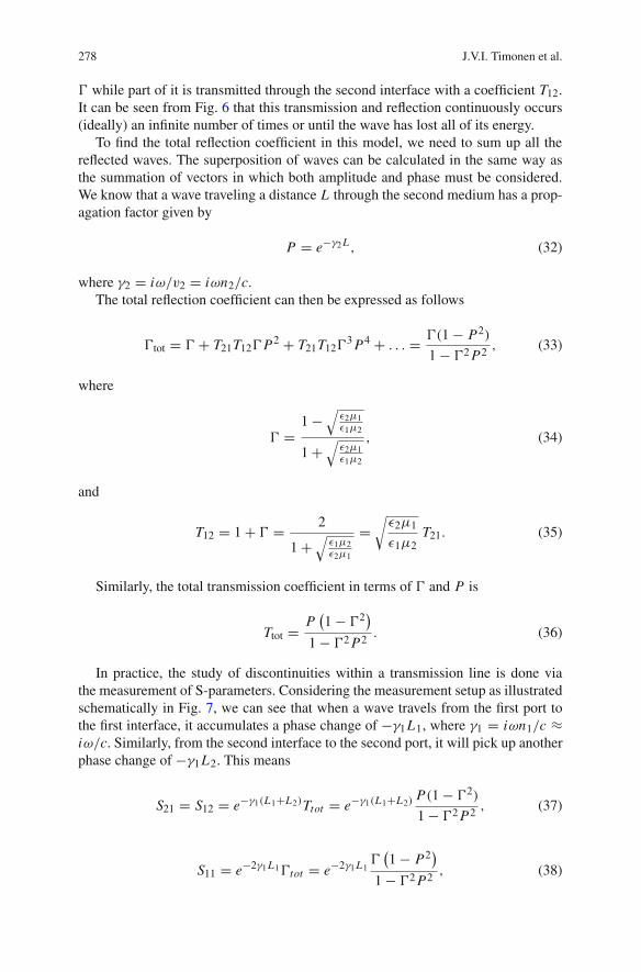
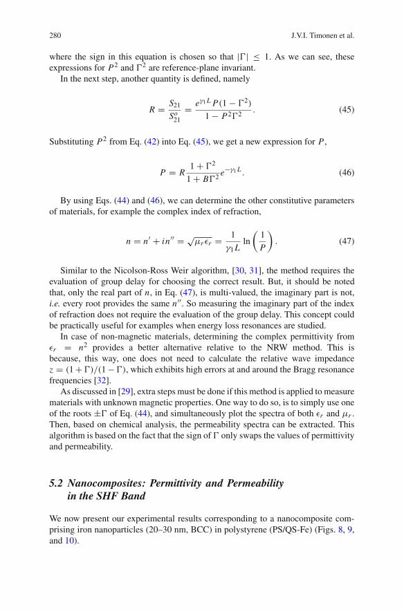
We now present our experimental results corresponding to a nanocomposite com-prising iron nanoparticles (20–30 nm, BCC) in polystyrene (PS/QS-Fe) (Figs. 8, 9,and 10).


Fig. 8 The complex relative permeability (real part in the left figure and imaginary part in the rightfigure) of PS/QS-Fe nanocomposites between 2 and 12 GHz. The three sets of points correspondto samples with 5% (squares), 10% (dots), and 15% (triangles) magnetic inclusions

–

–

–

Fig. 9 The complex relative permittivity (real part in the left figure and imaginary part in the rightfigure) of PS/QS-Fe nanocomposites between 2 and 12 GHz. The three sets of points correspondto samples with 5% (squares), 10% (dots), and 15% (triangles) magnetic inclusions

All the composites 5, 10 and 15% exhibited mild ferromagnetic resonancesbetween 6 and 8 GHz. These resonances correspond to the anisotropy fields between0.20 and 0.27 T. The expected anisotropy field calculated from bulk BCC ironmagnetocrystalline anisotropy is 56 mT. This large difference may be explained byadditional anisotropy components due to surface effects or particle-particle inter-actions. In the case of surface anisotropy the broadening of the resonance peakwould be due to the finite size distribution of the nanoparticles, and in the caseof particle-particle interactions due to variations of the polarizing field due to irreg-ular spatial arrangement and orientation of the particles. The Snoek limit (Eq. 13)predicts that no higher relative magnetic permeability than 8.5 can be achieved at5 GHz in (positive) uniaxial and cubic materials which are either bulk or compositescontaining spherical inclusions. According to the Bruggeman theory (Eq. 29) theeffective relative permeability is at maximum one sixth of 8.5 in a nanocomposite


–

––

––

–

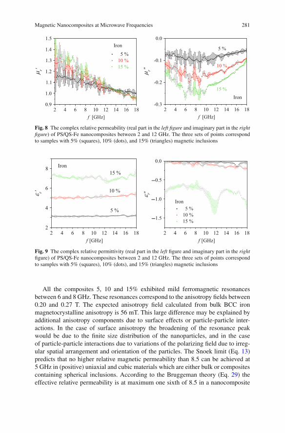
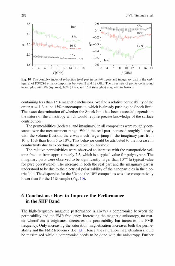
Fig. 10 The complex index of refraction (real part in the left figure and imaginary part in the rightfigure) of PS/QS-Fe nanocomposites between 2 and 12 GHz. The three sets of points correspondto samples with 5% (squares), 10% (dots), and 15% (triangles) magnetic inclusions

containing less than 15% magnetic inclusions. We find a relative permeability of theorder µ = 1.3 in the 15% nanocomposite, which is already pushing the Snoek limit.The exact determination of whether the Snoek limit has been exceeded depends onthe nature of the anisotropy which would require precise knowledge of the surfacecontribution.

The permeabilities (both real and imaginary) in all composites were roughly con-stants over the measurement range. While the real part increased roughly linearlywith the volume fraction, there was much larger jump in the imaginary part from10 to 15% than from 5 to 10%. This behavior could be attributed to the increase inconductivity due to exceeding the percolation threshold.

The relative permittivities were observed to increase with the nanoparticle vol-ume fraction from approximately 2.5, which is a typical value for polystyrene. Theimaginary parts were observed to be significantly larger than 10$4 (a typical valuefor pure polystyrene). The increase in both the real part and the imaginary part isunderstood to be due to the electrical polarizability of the nanoparticles in the elec-tric field. The dispersion for the 5% and the 10% composites was also comparativelylower than for the 15% sample (Fig. 10).

6 Conclusions: How to Improve the Performancein the SHF Band

The high-frequency magnetic performance is always a compromise between thepermeability and the FMR frequency. Increasing the magnetic anisotropy, no mat-ter wherefrom it originates, decreases the permeability but increases the FMRfrequency. Only increasing the saturation magnetization increases both the perme-ability and the FMR frequency (Eq. 13). Hence, the saturation magnetization shouldbe maximized while a compromise needs to be done with the anisotropy. Further


degree of freedom stems from the shape of the magnetic inclusions. It is well knownthat the resonance frequency of an arbitrary magnetic body with the demagnetizationfactors Nx , Ny and Nz is given by the Kittel formula [12]

fFMR = (2#)$1$

89HA + (Nx $ Nz) MS

: 9HA +

(Ny $ Nz

)MS

:, (48)

from which the well known resonance formulas for bulk, film, rod and sphere canbe derived ($ is the gyromagnetic constant, defined as in Eq. (6)). In the cases ofspheres (Nx = Ny = Nz = 1/3) and bulk material (Nx = Ny = Nz = 0), theresonance frequency is directly proportional to the anisotropy field (as was assumedin Subsection 2.2). In the infinite rod limit (Nx = Ny = 1/2, Nz = 0) the FMRfrequency is linearly proportional to the saturation magnetization (assuming thatMS 1 HA) and in the thin film limit (Nx = Ny = 0, Nz = 1) to the square rootof the saturation magnetization and the anisotropy field (assuming that MS 1 HA).Even in the case of HCP cobalt, which has a high anisotropy field of µ0 HA #0.63 T, the highest resonance frequency is obtained in the non-isotropic geometries,namely the infinite rod and the thin film. The same conclusion is valid for the BCCiron (µ0 HA # 56 mT), and the FCC nickel (µ0 HA # 16 mT). However, due tothe surface anisotropy, in the end the anisotropy field in nanoscale rods, spheresand films can be much larger than in bulk. It should be understood that the FMRfrequency depends on the shape of the magnetic inclusions, but obtaining qualitativeresults from calculations without knowing the surface anisotropy is not possible(as already pointed out in Sect. 2.2). In addition, the FMR frequency depends onparticle-particle interactions.

The volume fraction of the inclusions has obviously an effect on both theresonance frequency and the permeability. The permeability of a nanocompositewith spherical inclusions can be calculated directly from the Bruggeman theory(Sect. 3.2) but in all the other cases the Bruggeman equation must be solved itera-tively and self-consistently with the Landau-Lifshitz equation [33]. The results fromsuch calculations indicate that (1) the FMR frequency of a nanocomposite contain-ing spherical inclusion does not depend on the volume fraction and (2) in all othercases the FMR frequency smoothly varies from the single-inclusion limit to thehomogeneous bulk limit. Hence, the set of rules for predicting the high-frequencymagnetic performance stated in Sect. 3.2 are valid only for spherical nanoparticles.As argued above, the FMR resonance is the lowest in the bulk and spherical particlelimits. The results presented in Sect. 5.2 agree with the literature in a sense that theFMR frequency was found out to vary only a little with the nanoparticle volumefraction. The small variation might be due to slight deviations from ideal sphericalform or due to the aggregation of the nanoparticles.

The magnetic performance in nanocomposites could be improved by taking allthe above considerations into account when designing the material. In addition, itis preferential to use monodisperse, single-crystal nanoparticles in order to observewell-defined resonance peaks. Without such information, quantitative evaluation ofthe magnetic performance is difficult. Also, the surface effects such as the surface


anisotropy have to be taken into account since nanoparticles have a huge surface-to-volume ratio compared to bulk materials. Because the magnitude and the symmetryof the surface anisotropy is difficult to calculate, it cannot be taken in practice intoconsideration before the measurement. Instead, it is the deviation of the observedFMR frequency from the value expected from bulk magnetocrystalline anisotropythat indicates the magnitude of the surface anisotropy. After having decided thetarget permeability and resonance frequency and having approximated the type andthe volume fraction of the magnetic inclusions, one still needs to find the appro-priate processing route which can lead to such a nanocomposite. As argued in thisarticle, and also accepted in literature, homogeneous blends of plain nanoparticlesin polymers are almost impossible to achieve even at the lowest filling ratios. In thehigh-frequency applications the role of the nanoparticles is not just an additive sincethe practical volume fractions (from the application perspective) begin from 10%.Hence, the nanoparticles should be a supporting part of the nanocomposite – not anadditive.

Suppressing the large permittivity and dielectric loss will be a difficult task. Theimaginary losses can be reduced by using single-crystal nanoparticles in which theconduction electron scattering is suppressed. Tackling the real part is much moredifficult, since all metallic nanoparticles are highly conductive and their polarizabil-ity should of the same order.

Acknowledgements This work was supported by the Finnish Funding Agency for Technologyand Innovation (TEKES). G.S.P. would like to acknowledge also partial support from the Academyof Finland (Acad. Res. Fellowship 00857 and projects 129896, 118122, and 135135). K.C. wishesto thank the Thailand Commission on Higher Education for financial support.

References

1. Y. Shirakata et al., High permeability and low loss Ni-Fe composite material for high-frequency applications. IEEE Trans. Magn. 44, 2100 (2008)

2. R.C. Hansen, M. Burke, Antennas with magneto-dielectrics. Microw. Opt. Technol. Lett. 26,75 (2000)

3. R.A. Waldron, Ferrites: An Introduction for Microwave Engineers, (Van Nostrand, London,1961)

4. Super high frequency (2009), http://en.wikipedia.org/wiki/Super_high_frequency5. S. Sun et al., Monodisperse FePt nanoparticles and ferromagnetic FePt nanocrystal superlat-

tices. Science 287, 1989 (2000)6. V.F. Puntes et al., Colloidal nanocrystal shape and size control: the case of cobalt. Science

291, 2115 (2001)7. S. Moerup, M.F. Hansen, Fundamentals and Theory, in Handbook of Magnetism and Advanced

Magnetic Materials, ed. by H. Kronmueller, S. Parkin (Wiley, New York, NY, 2007)8. L.Z. Wu et al., Studies of high-frequency magnetic permeability of rod-shapes CrO2 nanopar-

ticles. Phys. Stat. Sol. 204, 755 (2006)9. C. Desvaux et al., Multimillimetre-large superlattices of air-stable iron-cobalt nanoparticles.

Nat. Mater. 4, 750 (2005)10. S. Chikazumi, Physics of Ferromagnetism (Oxford University Press, New York, 1997)11. R.C. O’Handley, Modern Magnetic Materials (Wiley, New York, NY, 2000)


12. C. Kittel, Introduction to Solid State Physics (Wiley, New York, NY, 1971)13. C.M. Sorensen, Magnetism in Nanoscale Materials in Chemistry, ed. by K.J. Klabunce

(Wiley-IEEE, New York, NY, 2001)14. S.J. Steinmuller et al., Effect of substrate roughness on the magnetic properties of thin fcc Co

films. Phys. Rev. B 76, (2007)15. P.K. George, E.D. Thompson, Exchange stiffness in hexagonal cobalt. Phys. Rev. Lett. 24,

1431 (1970)16. J.L. Snoek, Dispersion and absorption in magnetic ferrites at frequencies above one Mc/s.

Physica 15, 207 (1948)17. L. Landau, E. Lifshitz, On the theory of the dispersion of magnetic permeability in ferromag-

netic bodies. Phys. Z. Sowjetunion 8, (1935)18. G.H. Jonker et al., Philips Tech. Rev. 18, 1956 (1956)19. R. Krishnamoorti, R.A. Vaia, Polymer nanocomposites. J. Polymer Sci. B: Polymer Phys. 45,

3252 (2007)20. M.E. Mackay et al., General strategies for nanoparticle dispersion. Science 311, 1740 (2006)21. A.C. Balazs, S. Chandralekha, Effect of polymer architecture on the miscibility of poly-

mer/clay mixtures. Polymer Int. 49, 469 (2000)22. E. Glogowski et al., Functionalization of nanoparticles for dispersion in polymers and assem-

bly in fluids. J. Polymer Sci. A: Polymer Chem. 44, 5076 (2006)23. A.H. Latham, M.E. Williams, Controlling transport and chemical functionality of magnetic

nanoparticles. Acc. Chem. Res. 41, 411 (2008)24. J. Israelachvili, Intermolecular and Surface Forces (Academic, London, 1985)25. J.A. Pomposo et al., Key role of entropy in nanoparticle dispersion: polystyrene-

nanoparticle/linear-polystyrene nanocomposites as a model system. Phys. Chem. Chem. Phys.10, 650 (2007)

26. C. Barnes et al., Spontaneous formation of an exfoliated polystyrene-clay nanocompositeusing a star-shaped polymer. J. Am. Chem. Soc. 126, 8118 (2004)

27. Sihvola, Electromagnetic Mixing Formulas and Applications (The Institution of ElectricalEngineers, 1999)

28. J.H. Paterson et al., Complex permeability of soft magnetic ferrite/polyester resin compositesat frequencies above 1 MHz. J. Magn. Magn. Mater. 196–197, 394 (1999)

29. K. Chalapat, K. Sarvala, J. Li, G.S. Paraoanu, Wideband reference-plane invariant method formeasuring electromagnetic parameters of materials. IEEE Trans. Microw. Theory Tech. 57,2257 (2009)

30. A.M. Nicolson, G.F. Ross, Measurement of the intrinsic properties of materials by time-domain techniques. IEEE Trans. Instrum. Meas. IM-19, 377–382 (1970)

31. William B. Weir, Automatic measurement of complex dielectric constant and permeability atmicrowave frequencies. Proc. IEEE, 62, 33–36 (1974)

32. A.-H. Boughriet, C. Legrand, A. Chapoton, Noniterative stable transmission/reflection methodfor low-loss material complex permittivity determination. IEEE Tran. Microw. Theory Tech.45, 52–57 (1997)

33. R. Ramprasad et al., Fundamental limits of soft magnetic particle composites for high fre-quency applications. Phys. Stat. Sol. 233, 31 (2002)

34. H.P. Klug, L.E. Alexander, X-Ray Diffraction Procedures (Wiley, New York, NY, 1954)35. Å. Björck, Numerical methods for least squares problems, (SIAM, Philadelphia, 1996)

Documents

Magnetic Nanocomposites at Microwave Frequenciesrras/publications/21.pdf · Magnetic Nanocomposites at Microwave Frequencies 259 magnetic granularmaterials. A granular material is