t57

1

Magnetic Injection of Nanoparticles into Rat Inner Ears at a Human Head Working Distance

Azeem Sarwar1,3*, Roger Lee2,3, Didier A. Depireux2,3, Benjamin Shapiro1,2,3

1Fischell Department of Bioengineering, 2Institute for Systems Research, 3University of Maryland at College Park; *Corresponding author: azeem@umd.edu

Due to the physics of magnetic fields and forces, any single magnet will always attract or pull-in magnetically-responsive particles. However, there are a variety of clinical needs where it is advantageous to be able to push away or ‘magnetically inject’ therapeutic particles. Here we focus on magnetic injection to treat inner-ear diseases. The inner ear is behind the blood-ear barrier, meaning, blood vessels that supply blood to the inner ear have vessel walls that are impermeable and prevent drugs from exiting the vessels and reaching inner ear tissues. In our prior work, we showed that a simple four-magnet system could successfully push nanoparticles from the middle into the inner ear, thus circumventing the blood-ear barrier. That first-generation system could only push at a 2 cm distance: a range sufficient for rat experiments but not appropriate for adult human patients whose face-to-middle-ear distance varies from 3 to 5 cm. Here we demonstrate an optimal two-magnet system that can push at 3 to 5 cm distances. The system is designed using semi-definite quadratic programming which guarantees a globally optimal magnet configuration, is fabricated, characterized in detail, compared to theory, and then tested in rat experiments but now at a human 4 cm working distance.

Index Terms— Halbach magnet design, inner ear, magnetic nanoparticles, magnetic pushing

I. INTRODUCTION

herapeutic magnetizable nanoparticles can be manipulated by external magnets to direct drugs to regions of disease: to tumors [1–3], infections [4], and blood clots [5].

Magnetic targeting has allowed in-vivo focusing of systemically administered drugs [6–12], polymer capsules and liposomes [13-14], as well as gene therapy [15] and magnetized stem-cells [16].

Due to the physics of magnetic fields and forces, single magnets, whether permanent or electro-magnetic, attract ferromagnetic particles [17–19]. Hence the majority of prior magnetic systems have been designed to pull in or attract therapeutic particles to target regions [20–26]. For example, magnets have been held next to inoperable but shallow breast, head, and neck tumors to capture and concentrate chemotherapy in cancer patients [1,9]. It is, however, also possible to use two or more magnets to push away or “magnetically inject” particles [27]. Magnetic injection can be useful for situations where magnetic pull is impractical, inaccurate, insufficient, or otherwise undesirable due to anatomy or treatment constraints. For example, push can be used to direct therapies to the back of the eye [17-18] and into the inner ear [30–32] by using a magnet system that need only push over a short distance, instead of the much stronger system that would be required to create the same magnetic forces by pulling through the entire width of the human head [31].

In this paper we focus on improving magnetic push to treat inner ear diseases. There are a variety of inner ear diseases – such as sudden sensorineural hearing loss (SSHL), tinnitus (a loud ringing or roaring in the ears), and Meniere’s disease [33] – which respectively affect 5-20,000 [34], 15 million [35] and 600,000 [36] people per year in the United States. While it is thought that effective drugs are available (e.g. steroids), these drugs cannot reach the inner ear [43-44] because the inner ear

Fig. 1: Magnetic pulling versus pushing for ear [30] magnetic treatments. To magnetically direct drugs to the inner ear (A,B), one can either magnetically push over a short distance or pull over a much longer distance. Since magnetic forces fall off quickly with distance from magnets [39], pushing significantly outperforms pulling for comparable systems (×20 more push than pull force for the inner ear using 1 Tesla magnets [31]). In the schematic, the treatment target is shown in red, distances in purple, nanoparticles in black, and pull and push magnets in yellow and blue respectively.

(which comprises the cochlea, the vestibule and the semi-circular canals) is isolated by the blood-ear barrier [40], which is similar to the blood-brain barrier. All vessels that bring blood to the inner ear have vessel walls that are largely impermeable even to the smallest drug molecules [41]. Thus drugs that are taken orally or are injected into the blood-stream either do not elute or elute only poorly out into inner ear tissues [42].

Although it is possible to safely reach the middle ear by mechanical means – for example by injecting drugs with a syringe through the ear drum into the middle ear [45, 47–50] (the ear drum heals after the injection [46–48]) – it is not possible to do the same for the inner ear. As shown in Fig. 2, to reach the inner ear from the outside requires first going through the ear drum and then through either the round window membrane (RWM) or the oval window membrane (OWM). There is no line-of-sight from outside the human ear to the RWM and OWM, and most of the OWM is covered by

T

t57

2

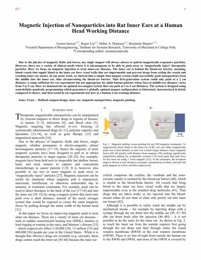
Fig. 2: Schematic of external, middle, and inner ear, and a cross section through the window membranes. A) The inner ear is located approximately 4 cm away from the outside of the human face. B) Magnified view of the middle ear. The oval and round window membranes that lead to the inner ear are marked by ‘OWM’ and ‘RWM’. C) The inner ear consists of the cochlea and the vestibular loops. D) Each of the window membranes, the RWM or the OWM, is composed of connective tissue sandwiched between layers of cuboidal epithelium cells. These membranes are approximately 70 m thick in humans (and 16 m thick in rats).

a small bone. Further, puncturing either of these delicate membranes would irreversibly destroy hearing. An alternate option is to deliver a large dose of drugs into the middle ear and wait for passive diffusion into the inner ear. However, diffusion through the RWM and OWM membranes is limited [54-55] and this treatment results in a steep drug concentration gradient inside the cochlea leading to too-high concentrations in the base of the cochlea with too-low concentrations in the region of trauma [37]. In summary, there is currently no drug delivery method that is both safe and effective for the inner ear, as shown schematically by Fig. 3 taken from the Salt and Plontke review article [37].

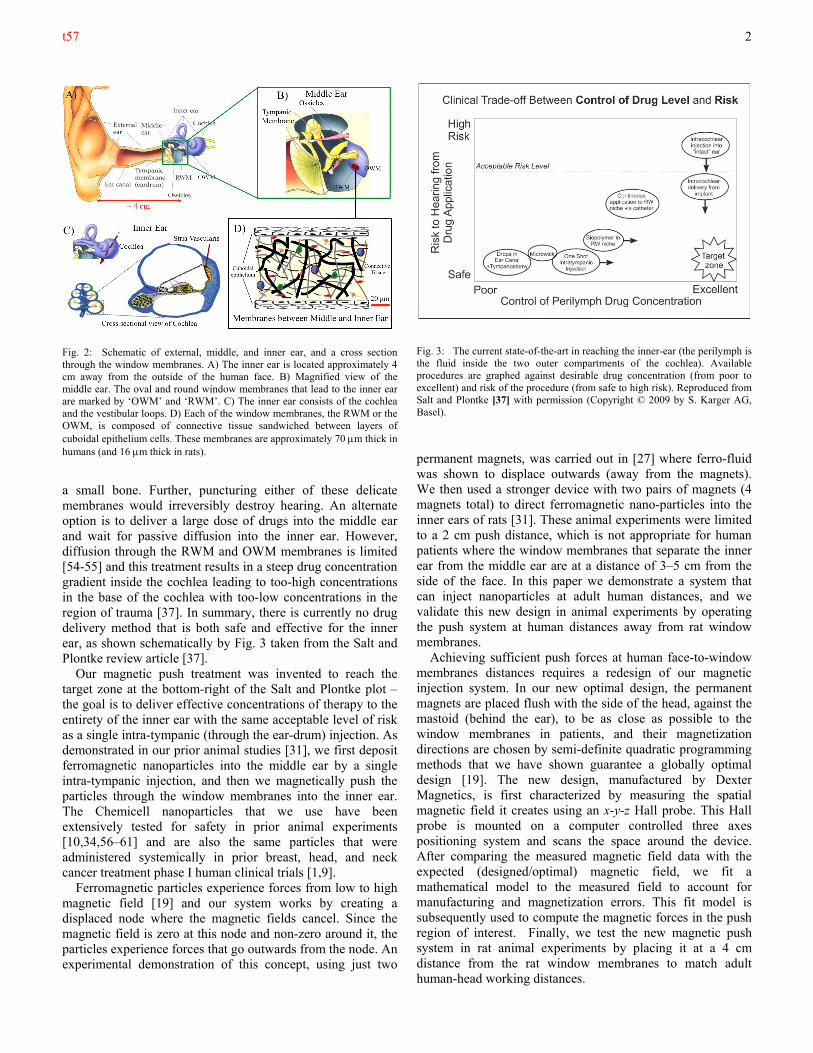
Our magnetic push treatment was invented to reach the target zone at the bottom-right of the Salt and Plontke plot – the goal is to deliver effective concentrations of therapy to the entirety of the inner ear with the same acceptable level of risk as a single intra-tympanic (through the ear-drum) injection. As demonstrated in our prior animal studies [31], we first deposit ferromagnetic nanoparticles into the middle ear by a single intra-tympanic injection, and then we magnetically push the particles through the window membranes into the inner ear. The Chemicell nanoparticles that we use have been extensively tested for safety in prior animal experiments [10,34,56–61] and are also the same particles that were administered systemically in prior breast, head, and neck cancer treatment phase I human clinical trials [1,9].

Ferromagnetic particles experience forces from low to high magnetic field [19] and our system works by creating a displaced node where the magnetic fields cancel. Since the magnetic field is zero at this node and non-zero around it, the particles experience forces that go outwards from the node. An experimental demonstration of this concept, using just two

Fig. 3: The current state-of-the-art in reaching the inner-ear (the perilymph is the fluid inside the two outer compartments of the cochlea). Available procedures are graphed against desirable drug concentration (from poor to excellent) and risk of the procedure (from safe to high risk). Reproduced from Salt and Plontke [37] with permission (Copyright © 2009 by S. Karger AG, Basel).

permanent magnets, was carried out in [27] where ferro-fluid was shown to displace outwards (away from the magnets). We then used a stronger device with two pairs of magnets (4 magnets total) to direct ferromagnetic nano-particles into the inner ears of rats [31]. These animal experiments were limited to a 2 cm push distance, which is not appropriate for human patients where the window membranes that separate the inner ear from the middle ear are at a distance of 3–5 cm from the side of the face. In this paper we demonstrate a system that can inject nanoparticles at adult human distances, and we validate this new design in animal experiments by operating the push system at human distances away from rat window membranes.

Achieving sufficient push forces at human face-to-window membranes distances requires a redesign of our magnetic injection system. In our new optimal design, the permanent magnets are placed flush with the side of the head, against the mastoid (behind the ear), to be as close as possible to the window membranes in patients, and their magnetization directions are chosen by semi-definite quadratic programming methods that we have shown guarantee a globally optimal design [19]. The new design, manufactured by Dexter Magnetics, is first characterized by measuring the spatial magnetic field it creates using an x-y-z Hall probe. This Hall probe is mounted on a computer controlled three axes positioning system and scans the space around the device. After comparing the measured magnetic field data with the expected (designed/optimal) magnetic field, we fit a mathematical model to the measured field to account for manufacturing and magnetization errors. This fit model is subsequently used to compute the magnetic forces in the push region of interest. Finally, we test the new magnetic push system in rat animal experiments by placing it at a 4 cm distance from the rat window membranes to match adult human-head working distances.

t57

3

II. PHYSICS FOR MAGNETIC PUSH

The magnetic force on a single ferro-magnetic particle is [57–60]

(1) 3 3 2

0 04 2

3 1 3 3 1 3

T

M

a H aF H H

x

where H

is the magnetic intensity [with units A/m], χ is the magnetic susceptibility, and μo = is the permeability of a vacuum, a is the radius of the particle [m], is the gradient operator [with units 1/m], and xH

/ is the

Jacobian matrix of H

and both are evaluated at the location of the particle. The first relation, which is more common in the magnetic drug delivery literature, shows that a spatially varying magnetic field ( 0/ xH

) is required to create

magnetic forces. It also shows that the force on a single particle is directly proportional to its volume. The second relation, which is equivalent to the first one by the chain rule, states that the force on particles is along the gradient of the magnetic field intensity squared – i.e. a ferro-magnetic particle will always experience a force from low to high applied magnetic field. Around a single magnet, 2|| ||H

is largest

closest to the magnet, and thus the magnetic force is always directed towards the magnet. This is why a single magnet can only attract or pull-in para-, ferro-, or super-magnetic particles towards it.

However, two or more magnets can be arranged to create a push force. Magnet system design can only change the magnetic field: in the second relation it can only modify

2|||| H

since all the other terms depend on the size and

material properties of the nanoparticles. Thus, to create an outward push force, 2|| ||H

must be made to increase going

away from the system of magnets. A simple way to achieve this is to create a local magnetic field minimum at a distance – the magnetic field strength will increase outwards from this minimum and create outward forces.

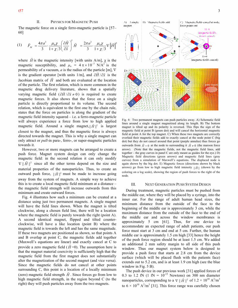
Fig. 4 illustrates how such a minimum can be created at a distance using just two permanent magnets. A single magnet will have the field lines shown. When the magnet is tilted clockwise, along a chosen field line, there will be a location where the magnetic field is purely towards the right (point A). A second identical magnet, flipped and tilted counter-clockwise, will have a like location (point B) where the magnetic field is towards the left and has the same magnitude. If these two magnets are positioned as shown, so that points A and B overlap at point C, the magnetic fields add together (Maxwell’s equations are linear) and exactly cancel at C to provide a zero magnetic field ( H

=0). The assumption here is

that the magnet material coercivity is sufficiently high that the magnetic field from the first magnet does not substantially alter the magnetization of the second magnet (and vice versa). Since the magnetic fields do not cancel at other points surrounding C, this point is a location of a locally minimum (zero) magnetic field strength H

. Since forces go from low to

high magnetic field strength, in the region beyond C (to the right) they will push particles away from the two magnets.

Fig. 4: Two permanent magnets can push particles away. A) Schematic field lines around a single magnet magnetized along its length. B) The bottom magnet is tilted up and its polarity is reversed. This flips the sign of the magnetic field at point B (green dot) and will cancel the horizontal magnetic field at point A for the top magnet. C) When these two magnets are correctly overlaid their magnetic fields add to exactly cancel at the node point C (big dot) but they do not cancel around that point (purple annulus) thus forces go outwards from 0H

at the node to surrounding it 0H

(the maroon force

arrow). (Note that the magnetic fields, not the magnetic field lines, add together – the gray curves in panel C are only meant as guides for the eye.) D) Magnetic field directions (green arrows) and magnetic field lines (gray curves) from a simulation of Maxwell’s equations. The displaced node is again shown by the big dot. E) Magnetic forces (directions shown by black arrows) go from low to high magnetic field intensity |||| H

(shown by the

coloring on a log scale), showing the region of push forces to the right of the node.

III. NEXT GENERATION PUSH SYSTEM DESIGN

During treatment, magnetic particles must be pushed from the middle ear, where they will be placed by a syringe, into the inner ear. For the range of adult human head sizes, the minimum distance from the outside of the face to the beginning of the middle ear is approximately 3 cm, while the maximum distance from the outside of the face to the end of the middle ear and across the window membranes is approximately 5 cm [61]. Thus, for one device to accommodate an expected range of adult patients, our push force must start at 3 cm and end at 5 cm. Further, the human middle ear is approximately 1.5 cm high [33] hence the height of the push force region should be at least 1.5 cm. We added an additional 2 mm safety margin to all side of this push window. Thus our magnet system below is designed to provide a push force that starts at 2.8 cm from the device surface (which will be placed flush with the patients face) extends out to 5.2 cm, and is at least 1.9 cm high (see the blue window in Fig. 5 B).

The push device in our previous work [31] applied forces of 0.3 to 1.2 fN (1 fN = 10-15 Newtons) on 300 nm diameter nanoparticles, corresponding to a 2|||| H

of 1.2 × 1010 A2/m3

to 6 × 1010 A2/m3 [31]. This force range was carefully chosen

t57

4

by first doing a succession of simpler pull experiments where a single magnet was placed at a sequence of distances from particles in the rat’s middle ear. It was found that when pull forces were too weak (< 0.3 fN) they did not transport a significant amount of particles into the inner ear of the rats, while when the pull forces were too strong (> 1.2 fN) they embedded nanoparticles into the walls of the cochlea. The details of these prior calibration pull experiments are summarized in the Appendix A.

A. Optimal Two-Magnet System Design and Manufacture

For ease of fabrication, we considered a two magnet system with two identical magnets side by side, each having a height of 11.25 cm (along the z-axis), width of 5.62 cm (along the y-axis), and a thickness of 4.44 cm (along the x-axis). We employed the methods described in [19] to determine the optimal magnetization directions of these two magnets to generate maximum push force at a distance of 4 cm from the yz face of the magnet. We briefly describe below how this problem was mathematically formulated and solved along the lines of [19].

The task is to select the magnetization directions to maximize push forces on particles located at 4 cm from the face of magnet assembly given a practical maximum allowable magnetic field strength. Since we used grade N52 NdFeB magnets, the maximum magnetization of each magnet was restricted to 1.48 Tesla [62]. The magnetic field around a uniformly magnetized rectangular magnet is known analytically [63]. Let ),,( zyxA

, ),,( zyxB

, and ),,( zyxC

respectively represent the analytical expressions for the magnetic field around a rectangular magnet that is uniformly magnetized either along x, y, or z axis. Then the magnetic field created by the two magnet assembly at an external location (x0,y0,z0) is given by

(2)

),,(

),,(),,(

),,(

000

2

1000000

000

iiiii

iiiiiiiiiii

czbyaxC

czbyaxBczbyaxA

zyxH

where ai, bi, ci is the location of each rectangular magnet, and i, i, and γi are the design coefficients, and must satisfy the constraint αi

2+ βi2 +γi

2≤ 1.482. According to equation (1), the strength of the magnetic force experienced by a magnetic particle at a point (x0,y0,z0) is directly proportional to the gradient of the square of the magnetic field at that point. Simplify the notation to

(3) ),,( 000 iiiii czbyaxAA

(4) ),,( 000 iiiii czbyaxBB

and (5) ),,( 000 iiiii czbyaxCC

then squaring equation (2) and taking the gradient, the expression for ),,( 000

2 zyxH

becomes

(6)

)()(

)()()()(

)()()((

),,(2

1

2

1

0002

jijijiji

jijijijijijijiji

j ijijijijijiji

CCBC

ACCBBBAB

CABAAA

zyxH

since the gradient operator is linear, and the coefficients i, i, and γi are not functions of x, y, z and can therefore be pulled out of the summation. The design goal is to maximize magnetic push forces along the horizontal axis and, thus, the focus is solely on the horizontal component of

),,( 0002 zyxH

, which will be denoted by an x sub-script.

Define the vector p

as

(7) Tp 212121 ,,,,,:

and define the matrix P as

(8)

xCCCCBCBCACAC

CCCCBCBCACAC

CBCBBBBBABAB

CBCBBBBBABAB

CACABABAAAAA

CACABABAAAAA

P

)()()()()()(

)()()()()()(

)()()()()()(

)()()()()()(

)()()()()()(

)()()()()()(

:

211222122212

211121112111

211222122212

211121112111

221222122212

211121112111

Now xzyxH ),,( 000

2

can be written in compact form as

(9) pPpzyxH T

x

),,( 000

2 .

To include the αi

2+ βi2 +γi

2≤ 1.482 magnetization constraints, let Ki be a 6×6 matrix having 1/(1.482) at the locations (i,i) (2+i,2+i), and (4+i,4+i) and with zeros everywhere else. Then the element magnetization constraints can be written in matrix form as

(10) 1pKp iT

for all i=1,2. The push force optimization problem can, therefore, be stated as follows: maximize the quadratic cost

pPpT of equation (9) subject to the two constraints of

equation (10), one for each of the two magnets. The optimization problem is quadratic in the design variables and was solved using semi-definite relaxation [64] and the majorization method [65] yielding a provably globally optimum solution.

This optimal magnetization, along with the side-by-side arrangement of the magnets, worked out to be

1 ( 1.033, 1.060,0) TeslaM

and 2 ( 1.033, 1.060,0) TeslaM

,

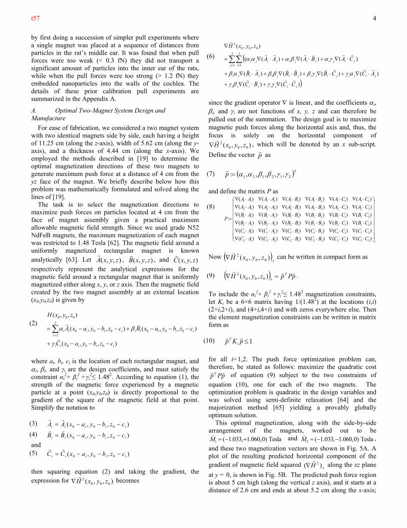
and these two magnetization vectors are shown in Fig. 5A. A plot of the resulting predicted horizontal component of the gradient of magnetic field squared

xH )( 2

along the xz plane

at y = 0, is shown in Fig. 5B. The predicted push force region is about 5 cm high (along the vertical z axis), and it starts at a distance of 2.6 cm and ends at about 5.2 cm along the x-axis;

t57

5

thus it overlaps the 2.8 to 5.2 cm horizontal extent and significantly exceeds the 1.9 cm vertical range desired for adult human patients. The push

xH )( 2

ranges between 1.2 ×

1010 A2/m3 and 6 × 1010 A2/m3 over the push region, and is 4.5 × 1010 A2/m3 at 4 cm away from the yz-face of the magnet. Thus this two-magnet design meets both the spatial extent requirements for human head sizes and the forces that were required to direct particles through the window membranes in prior rat experiments.

-5

0

5 -50

5

-5

0

5

y[cm]x[cm]

z[cm

]

Fig. 5: A) Schematic showing the placement and magnetization of the two magnets for the optimal push system. B) Plot of

xH )( 2

in the xz-plane at the

center of magnet. White arrows indicate the direction of the push forces, colors indicate the magnitude of

xH )( 2

in the push domain, white denotes

pull regions, and the underlying gray shows a sample ear anatomy. The spatial range of required push forces to accommodate adult patients is indicated by the blue window.

The designed magnetic system was manufactured by Dexter Magnetic Technologies using grade N52 NdFeB magnetic material, supplied by Vacuumschmelze GmbH & Co. Retaining the magnetization along the easy axis of the magnetic material results in a more stable and homogenous magnet as opposed to magnetizing at an angle different from the easy axis [66]. To achieve this for the design shown in Fig. 5, bigger blocks were cut by diamond cutting wheels and ground down using grinding wheels into angled rectangular blocks that had their easy magnetization directions along the desired angles. These cut pieces were then magnetized using a 6.5 inch diameter magnetizing coil (F-756 coil made by Magnetic Instrumentation) applying a magnetic field of 31.58 kG (3.15 Tesla) at 2000 V. The magnetized pieces were then glued together using Loctite 330 and Activator 7387. This glue layer was approximately 0.08 mm thick. The magnetic assembly was then partially coated by epoxy (Resinlab EP965 parts 1 &2) to further strengthen the magnet assembly.

IV. CHARACTERIZATION OF THE BUILT SYSTEM

In this section we discuss the characterization of the built magnetic system. We first discuss spatial measurements of the magnetic vector field in and around the push region. This measured magnetic field is compared with the designed field, and the mismatch between the two is analyzed. Then, a new mathematical model is fit to the measured magnetic field, and this model is used to quantify the push force and its range of action. The fitted model can be differentiated analytically to find the gradients of the magnetic field, and to thus calculate the applied forces, as compared to numerically differentiating noisy measured data which would lead to a less accurate quantification of the forces produced by the built system.

A. Magnetic Field Measurement

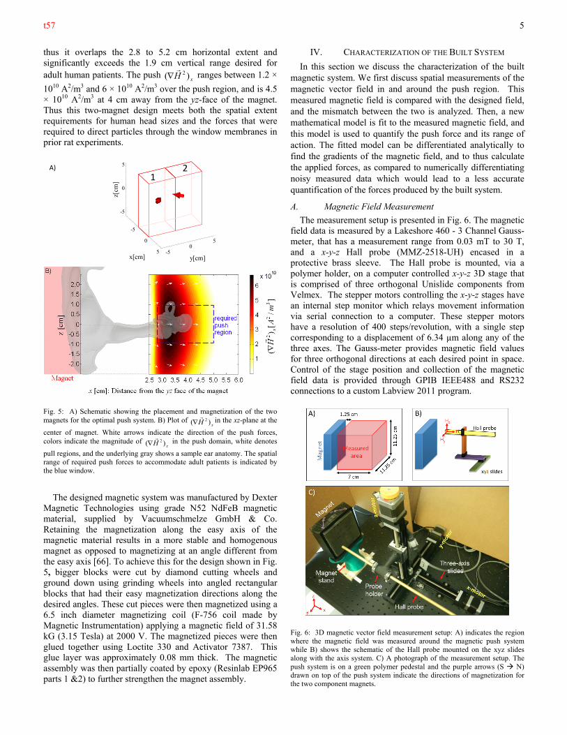
The measurement setup is presented in Fig. 6. The magnetic field data is measured by a Lakeshore 460 - 3 Channel Gauss-meter, that has a measurement range from 0.03 mT to 30 T, and a x-y-z Hall probe (MMZ-2518-UH) encased in a protective brass sleeve. The Hall probe is mounted, via a polymer holder, on a computer controlled x-y-z 3D stage that is comprised of three orthogonal Unislide components from Velmex. The stepper motors controlling the x-y-z stages have an internal step monitor which relays movement information via serial connection to a computer. These stepper motors have a resolution of 400 steps/revolution, with a single step corresponding to a displacement of 6.34 µm along any of the three axes. The Gauss-meter provides magnetic field values for three orthogonal directions at each desired point in space. Control of the stage position and collection of the magnetic field data is provided through GPIB IEEE488 and RS232 connections to a custom Labview 2011 program.

Fig. 6: 3D magnetic vector field measurement setup: A) indicates the region where the magnetic field was measured around the magnetic push system while B) shows the schematic of the Hall probe mounted on the xyz slides along with the axis system. C) A photograph of the measurement setup. The push system is on a green polymer pedestal and the purple arrows (S N) drawn on top of the push system indicate the directions of magnetization for the two component magnets.

A) 

1 2 

t57

6

The magnetic field was measured in a 7 cm × 11.25 cm × 11.25 cm region 1.25 cm away from the front face of the magnetic system, as shown in Fig. 6A. Measurements of the vector magnetic field were taken at a spacing of 2.08 mm along the y and z axes and at a spacing of 3 mm along the x-axis. The measured 3-dimensional magnetic vector field data at each point (Hx, Hy, and Hz) was then compared with the magnetic vector field theoretically predicted for the designed system.

Qualitatively, the measured and theoretically predicted magnetic fields match reasonably well. In the measured field there is a strong |||| H

minimum close to the predicted point

of cancellation as shown in Fig. 7 which presents contour plots of the magnetic field strength along a horizontal and vertical slice for the designed and the built push systems. Along the x-axis, the cancellation node can be seen to be at about 2.8 cm for the built system as opposed to the predicted location of 2.6 cm in the ideal design. Along the y-axis, it is at -0.1 cm for the built system as opposed to the predicted on-center (y = 0 cm) location. Likewise, along the z-axis it is at -0.3 cm for the built system as opposed to the anticipated centered (z = 0 cm) location

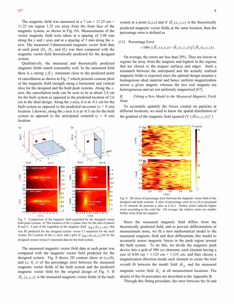
Fig. 7: Comparison of the magnetic field generated by the designed versus built push systems. A) The location of the xy-plane slice for the data of panels B and C. A plot of the logarithm of the magnetic field ||)0,,(||log yxH

that

was B) predicted for the designed system versus C) measured for the built system. D) Location of the xz slice, and a plot of ||),0,(||log zxH

for E) the

designed system versus F) measured data for the built system.

The measured magnetic vector field data at each point was compared with the magnetic vector field predicted for the designed system. Fig. 8 shows 2D contour slices at (x,y,0), and (x, 0, z) of the percentage error between the measured magnetic vector fields of the built system and the predicted magnetic vector field for the original design of Fig. 5. If

),,( zyxH F

is the measured magnetic vector fields of the built

system at a point (x,y,z) and if ),,( zyxHT

is the theoretically

predicted magnetic vector fields at the same location, then the percentage error is defined as

(11) Percentage Error

||),,(||||),,(),,(||100 zyxHzyxHzyxH FTF

.

On average, the errors are less than 20%. They are lowest at

regions far away from the magnets and highest in the regions that are closest to the magnet surfaces and edges. Such a mismatch between the anticipated and the actually realized magnetic fields is expected since the optimal design assumes a homogenous ideal material and hence uniform magnetization across a given magnet, whereas the two real magnets are heterogeneous and are not uniformly magnetized [67].

B. Fitting a New Model to the Measured Magnetic Field Data

To accurately quantify the forces created on particles at different locations, we need to know the spatial distribution of

the gradient of the magnetic field squared ( 2|| ( , , ) ||H x y z

).

Fig. 8: 2D slices of percentage error between the magnetic vector field of the designed and built systems. A slice of percentage error at (x,y,0) is presented in A) whereas B) presents a slice at (x,0,z). Darker colors indicate higher errors according to the scale bar. On average, the relative errors are smaller further away from the magnets.

Since the measured magnetic field differs from the

theoretically predicted field, and to prevent differentiation of measurement noise, we fit a new mathematical model to the measured magnetic field and then differentiate this model to accurately assess magnetic forces in the push region around the built system. To do this, we divide the magnetic push device into a grid of 500 xyz elements, each element having a size of 0.88 cm × 1.125 cm × 1.125 cm, and then choose a magnetization direction inside each element to create the best overall fit between the model field

MH

and the measured

magnetic vector field FH

at all measurement locations. The

details of this fit procedure are described in the Appendix B. Through this fitting procedure, the error between the fit and

t57

7

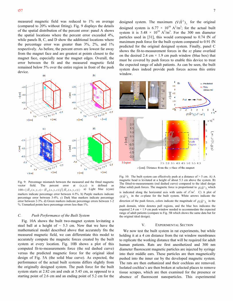
measured magnetic field was reduced to 1% on average (compared to 20% without fitting). Fig. 9 displays the details of the spatial distribution of the percent error: panel A shows the spatial locations where the percent error exceeded 4%, while panels B, C, and D show the additional locations where the percentage error was greater than 3%, 2%, and 1% respectively. As before, the percent errors are lowest far away from the magnet face and are greatest at points closest to the magnet face, especially near the magnet edges. Overall, the error between the fit and the measured magnetic field remained below 5% over the entire region in front of the push device.

Fig. 9: Percentage mismatch between the measured and the fitted magnetic vector field. The percent error at (x,y,z) is defined as

100 || ( , , ) ( , , ) || || ( , , ) ||F M FH x y z H x y z H x y z

. a) Light blue (cyan)

markers indicate percentage error between 4-5%. b) Purple markers indicate percentage error between 3-4%. c) Dark blue markers indicate percentage error between 2-3%. d) Green markers indicate percentage errors between 1-2 %. Unmarked points have percentage errors less than 1%.

C. Push Performance of the Built System

Fig. 10A shows the built two-magnet system levitating a steel ball at a height of ~ 5.3 cm. Now that we have the mathematical model described above that accurately fits the measured magnetic field, we can differentiate this model to accurately compute the magnetic forces created by the built system at every location. Fig. 10B shows a plot of this computed fit-to-measurements force (the red dashed curve) versus the predicted magnetic force for the original ideal design of Fig. 5A (the solid blue curve). As expected, the performance of the actual built systems differs slightly from the originally designed system. The push force for the built system starts at 2.82 cm and ends at 5.45 cm, as opposed to a starting point of 2.6 cm and an ending point of 5.2 cm for the

designed system. The maximum xH )( 2

for the original

designed system is 6.77 × 1010 A2/m3; for the actual built system it is 5.48 × 1010 A2/m3. For the 300 nm diameter particles used in [31], this would correspond to 0.74 fN of maximum push force for the built system compared to 0.91 fN predicted for the original designed system. Finally, panel C shows the fit-to-measurement forces in the xz plane overlaid on the desired 2.4 cm × 1.9 cm push window (blue box) that must be covered by push forces to enable this device to treat the expected range of adult patients. As can be seen, the built system does indeed provide push forces across this entire window.

Fig. 10: The built system can effectively push at a distance of > 5 cm. A) A magnetic bead is levitated at a height of about 5.3 cm above the system. B) The fitted-to-measurements (red dashed curve) compared to the ideal design (blue solid) push forces. The magnetic force is proportional to

xH )( 2

which

is indicated along the horizontal axis with units of A2/m3. C) A plot of

xH )( 2

in the zx-plane for the built system. White arrows indicate the

direction of the push forces, colors indicate the magnitude of xH )( 2

in the

push domain, white denotes pull regions, and the blue box indicates the required 2.4 cm × 1.9 cm push window needed to accommodate the expected range of adult patients (compare to Fig. 5B which shows the same data but for the original ideal design).

V. EXPERIMENTAL SECTION

We now test the built system in rat experiments, but while holding it at a 4 cm distance from the rat window membranes to replicate the working distance that will be required for adult human patients. Rats are first anesthetized and 300 nm diameter fluorescent magnetic particles are injected by syringe into their middle ears. These particles are then magnetically pushed into the inner ear by the developed magnetic system. The rats are then euthanized and their cochleas are removed. Isolated cochlea’s are then broken at selected places to remove tissue scrapes, which are then examined for the presence or absence of fluorescent nanoparticles. This experimental

t57

8

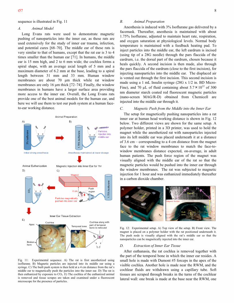
sequence is illustrated in Fig. 11

A. Animal Model

Long Evans rats were used to demonstrate magnetic pushing of nanoparticles into the inner ear, as these rats are used extensively for the study of inner ear trauma, infection, and potential cures [68–70]. The middle ear of these rats is very similar to that of humans, except that the rat ear is 3 to 4 times smaller than the human ear [71]. In humans, the middle ear is 15 mm high, and 2 to 6 mm wide; the cochlea forms a spiral shape, with an average axial length of 5 mm and a maximum diameter of 6.2 mm at the base, leading to a spiral length between 31 mm and 33 mm. Human window membranes are about 70 μm thick while rat window membranes are only 16 μm thick [72–74]. Finally, the window membranes in humans have a larger surface area providing more access to the inner ear. Overall, the Long Evans rats provide one of the best animal models for the human ear, and here we will use them to test our push system at a human face-to-ear working distance.

Fig. 11: Experimental sequence. A) The rat is first anesthetized using isoflurane. B) Magnetic particles are injected into its middle ear using a syringe. C) The built push system is then held at a 4 cm distance from the rat’s middle ear to magnetically push the particles into the inner ear. D) The rat is then euthanized by exposure to CO2. E) The cochlea of the euthanized animal is removed and tissue scrapes are taken and examined under a fluorescent microscope for the presence of particles.

B. Animal Preparation

Anesthesia is induced with 3% Isoflurane gas delivered by a facemask. Thereafter, anesthesia is maintained with about 1.75% Isoflurane, adjusted to maintain heart rate, respiration, and oxygen saturation at physiological levels. Normal body temperature is maintained with a feedback heating pad. To inject particles into the middle ear, the left eardrum is incised (using tip of a 28G needle) through the pars flaccida of the eardrum, i.e. the dorsal part of the eardrum, chosen because it heals quickly. A second incision is then made, also through the pars flaccida of the eardrum (close to the first incision), for injecting nanoparticles into the middle ear. The displaced air is vented out through the first incision. This second incision is made using a 1 mL Insulin syringe (28G x 1/2 in. BD Micro-Fine), and 70 µL of fluid containing about 5.7×1012 of 300 nm diameter starch coated red fluorescent magnetic particles (nano-screen MAG/R-D) obtained from Chemicell are injected into the middle ear through it.

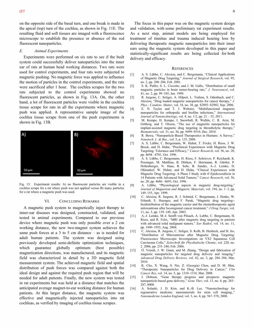
C. Magnetic Push from the Middle into the Inner Ear

The setup for magnetically pushing nanoparticles into a rat inner ear at human head working distance is shown in Fig. 12 below. Two different views are shown for the same setup. A polymer holder, printed in a 3D printer, was used to hold the magnet while the anesthetized rat with nanoparticles injected into its left middle ear was placed underneath it at a distance of 3.6 cm – corresponding to a 4 cm distance from the magnet face to the rat window membranes to match the face-to-window membranes distance expected, on-average, in adult human patients. The push force region of the magnet was visually aligned with the middle ear of the rat so that the magnetic particles would be pushed into the inner ear through the window membranes. The rat was subjected to magnetic injection for 1 hour and was euthanized immediately thereafter in a carbon dioxide chamber.

Fig. 12: Experimental setup. A) Top view of the setup. B) Front view. The magnet is placed on a polymer holder with the rat positioned underneath it. The push node is visually aligned with the rat’s middle ear so that the nanoparticles can be magnetically injected into the inner ear.

D. Extraction of Inner Ear Tissue

After euthanasia, the rat cochlea is removed together with the part of the temporal bone in which the inner ear resides. A small hole is made with Dumont #5 forceps in the apex of the visible cochlea. Another hole is made near the RWM, and the cochlear fluids are withdrawn using a capillary tube. Soft tissues are scraped through breaks in the turns of the cochlear lateral wall: one break is made at the base near the RWM, one

t57

9

on the opposite side of the basal turn, and one break is made in the apical (top) turn of the cochlea, as shown in Fig. 11E. The resulting fluid and soft tissues are imaged with a fluorescence microscope to establish the presence or absence of the red fluorescent nanoparticles.

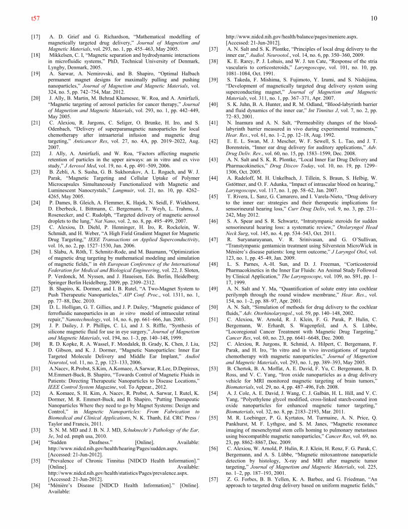
E. Animal Experiments

Experiments were performed on six rats to see if the built system could successfully deliver nanoparticles into the inner ear of rats at human head working distances. Two rats were used for control experiments, and four rats were subjected to magnetic pushing. No magnetic force was applied to influence the motion of particles in the control experiments, and the rats were sacrificed after 1 hour. The cochlea scrapes for the two rats subjected to the control experiments showed no fluorescent particles, as shown in Fig. 13A. On, the other hand, a lot of fluorescent particles were visible in the cochlea tissue scrape for rats in all the experiments where magnetic push was applied. A representative sample image of the cochlea tissue scrape from one of the push experiments is shown in Fig. 13B.

Fig. 13: Experiment results: A) no fluorescent particles are visible in a cochlea scrape for a rat where push was not applied versus B) many particles for a rat where a magnetic push was used.

VI. CONCLUDING REMARKS

A magnetic push system to magnetically inject therapy to inner-ear diseases was designed, constructed, validated, and tested in animal experiments. Compared to our previous device where magnetic push was only possible over a 2 cm working distance, the new two-magnet system achieves the same push forces at a 3 to 5 cm distance – as is needed for adult human patients. The system was designed using previously developed semi-definite optimization techniques, which guarantee globally optimum (best possible) magnetization directions, was manufactured, and its magnetic field was characterized in detail by a 3D magnetic field measurement system. The achieved magnetic field and spatial distribution of push forces was compared against both the ideal design and against the required push region that will be needed for adult patients. Finally, the new system was tested in rat experiments but was held at a distance that matches the anticipated average magnet-to-ear working distance for human patients. At this larger distance, the magnetic system was effective and magnetically injected nanoparticles into rat cochleas, as verified by imaging of cochlea tissue scrapes.

The focus in this paper was on the magnetic system design and validation, with some preliminary rat experiment results. As a next step, animal models are being employed for treatment of tinnitus and trauma induced hearing loss by delivering therapeutic magnetic nanoparticles into their inner ears using the magnetic system developed in this paper and statistically-significant results are being collected for both delivery and efficacy.

REFERENCES

[1] A. S. Lübbe, C. Alexiou, and C. Bergemann, “Clinical Applications of Magnetic Drug Targeting,” Journal of Surgical Research, vol. 95, no. 2, pp. 200–206, Feb. 2001.

[2] S. K. Pulfer, S. L. Ciccotto, and J. M. Gallo, “Distribution of small magnetic particles in brain tumor-bearing rats,” J. Neurooncol, vol. 41, no. 2, pp. 99–105, Jan. 1999.

[3] R. Jurgons, C. Seliger, A. Hilpert, L. Trahms, S. Odenbach, and C. Alexiou, “Drug loaded magnetic nanoparticles for cancer therapy,” J. Phys.: Condens. Matter, vol. 18, no. 38, pp. S2893–S2902, Sep. 2006.

[4] E. N. Taylor and T. J. Webster, “Multifunctional magnetic nanoparticles for orthopedic and biofilm infections,” International Journal of Nanotechnology, vol. 8, no. 1/2, pp. 21 – 35, 2011.

[5] M. Kempe, H. Kempe, I. Snowball, R. Wallén, C. R. Arza, M. Götberg, and T. Olsson, “The use of magnetite nanoparticles for implant-assisted magnetic drug targeting in thrombolytic therapy,” Biomaterials, vol. 31, no. 36, pp. 9499–9510, Dec. 2010.

[6] R. Bawa, “Nanoparticle-Based Therapeutics in Humans: A Survey,” Nanotech. L. & Bus., vol. 5, p. 135, 2008.

[7] A. S. Lübbe, C. Bergemann, W. Huhnt, T. Fricke, H. Riess, J. W. Brock, and D. Huhn, “Preclinical Experiences with Magnetic Drug Targeting: Tolerance and Efficacy,” Cancer Research, vol. 56, no. 20, pp. 4694 –4701, Oct. 1996.

[8] A. S. Lübbe, C. Bergemann, H. Riess, F. Schriever, P. Reichardt, K. Possinger, M. Matthias, B. Dörken, F. Herrmann, R. Gürtler, P. Hohenberger, N. Haas, R. Sohr, B. Sander, A.-J. Lemke, D. Ohlendorf, W. Huhnt, and D. Huhn, “Clinical Experiences with Magnetic Drug Targeting: A Phase I Study with 4′-Epidoxorubicin in 14 Patients with Advanced Solid Tumors,” Cancer Research, vol. 56, no. 20, pp. 4686 –4693, Oct. 1996.

[9] A. Lübbe, “Physiological aspects in magnetic drug-targeting,” Journal of Magnetism and Magnetic Materials, vol. 194, no. 1–3, pp. 149–155, Apr. 1999.

[10] C. Alexiou, R. Jurgons, R. J. Schmid, C. Bergemann, J. Henke, W. Erhardt, E. Huenges, and F. Parak, “Magnetic drug targeting--biodistribution of the magnetic carrier and the chemotherapeutic agent mitoxantrone after locoregional cancer treatment,” J Drug Target, vol. 11, no. 3, pp. 139–149, Apr. 2003.

[11] A.-J. Lemke, M.-I. Senfft von Pilsach, A. Lubbe, C. Bergemann, H. Riess, and R. Felix, “MRI after magnetic drug targeting in patients with advanced solid malignant tumors,” Eur Radiol, vol. 14, no. 11, pp. 1949–1955, Aug. 2004.

[12] C. Alexiou, R. Jurgons, C. Seliger, S. Kolb, B. Heubeck, and H. Iro, “Distribution of Mitoxantrone after Magnetic Drug Targeting: Fluorescence Microscopic Investigations on VX2 Squamous Cell Carcinoma Cells,” Zeitschrift für Physikalische Chemie, vol. 220, no. 2_2006, pp. 235–240, Feb. 2006.

[13] O. Veiseh, J. W. Gunn, and M. Zhang, “Design and fabrication of magnetic nanoparticles for targeted drug delivery and imaging,” Advanced Drug Delivery Reviews, vol. 62, no. 3, pp. 284–304, Mar. 2010.

[14] K. Cho, X. Wang, S. Nie, Z. (Georgia) Chen, and D. M. Shin, “Therapeutic Nanoparticles for Drug Delivery in Cancer,” Clin Cancer Res, vol. 14, no. 5, pp. 1310–1316, Mar. 2008.

[15] J. Dobson, “Gene therapy progress and prospects: magnetic nanoparticle-based gene delivery,” Gene Ther, vol. 13, no. 4, pp. 283–287, 0000.

[16] A. Solanki, J. D. Kim, and K.-B. Lee, “Nanotechnology for regenerative medicine: nanomaterials for stem cell imaging.,” Nanomedicine London England, vol. 3, no. 4, pp. 567–578, 2008.

t57

10

[17] A. D. Grief and G. Richardson, “Mathematical modelling of magnetically targeted drug delivery,” Journal of Magnetism and Magnetic Materials, vol. 293, no. 1, pp. 455–463, May 2005.

[18] Mikkelsen, C. I, “Magnetic separation and hydrodynamic interactions in microfluidic systems,” PhD, Technical University of Denmark, Lyngby, Denmark, 2005.

[19] A. Sarwar, A. Nemirovski, and B. Shapiro, “Optimal Halbach permanent magnet designs for maximally pulling and pushing nanoparticles,” Journal of Magnetism and Magnetic Materials, vol. 324, no. 5, pp. 742–754, Mar. 2012.

[20] J. Ally, B. Martin, M. Behrad Khamesee, W. Roa, and A. Amirfazli, “Magnetic targeting of aerosol particles for cancer therapy,” Journal of Magnetism and Magnetic Materials, vol. 293, no. 1, pp. 442–449, May 2005.

[21] C. Alexiou, R. Jurgons, C. Seliger, O. Brunke, H. Iro, and S. Odenbach, “Delivery of superparamagnetic nanoparticles for local chemotherapy after intraarterial infusion and magnetic drug targeting,” Anticancer Res, vol. 27, no. 4A, pp. 2019–2022, Aug. 2007.

[22] J. Ally, A. Amirfazli, and W. Roa, “Factors affecting magnetic retention of particles in the upper airways: an in vitro and ex vivo study,” J Aerosol Med, vol. 19, no. 4, pp. 491–509, 2006.

[23] B. Zebli, A. S. Susha, G. B. Sukhorukov, A. L. Rogach, and W. J. Parak, “Magnetic Targeting and Cellular Uptake of Polymer Microcapsules Simultaneously Functionalized with Magnetic and Luminescent Nanocrystals,” Langmuir, vol. 21, no. 10, pp. 4262–4265, May 2005.

[24] P. Dames, B. Gleich, A. Flemmer, K. Hajek, N. Seidl, F. Wiekhorst, D. Eberbeck, I. Bittmann, C. Bergemann, T. Weyh, L. Trahms, J. Rosenecker, and C. Rudolph, “Targeted delivery of magnetic aerosol droplets to the lung,” Nat Nano, vol. 2, no. 8, pp. 495–499, 2007.

[25] C. Alexiou, D. Diehl, P. Henninger, H. Iro, R. Rockelein, W. Schmidt, and H. Weber, “A High Field Gradient Magnet for Magnetic Drug Targeting,” IEEE Transactions on Applied Superconductivity, vol. 16, no. 2, pp. 1527–1530, Jun. 2006.

[26] I. Slabu, A. Röth, T. Schmitz-Rode, and M. Baumann, “Optimization of magnetic drug targeting by mathematical modeling and simulation of magnetic fields,” in 4th European Conference of the International Federation for Medical and Biological Engineering, vol. 22, J. Sloten, P. Verdonck, M. Nyssen, and J. Haueisen, Eds. Berlin, Heidelberg: Springer Berlin Heidelberg, 2009, pp. 2309–2312.

[27] B. Shapiro, K. Dormer, and I. B. Rutel, “A Two-Magnet System to Push Therapeutic Nanoparticles,” AIP Conf. Proc., vol. 1311, no. 1, pp. 77–88, Dec. 2010.

[28] D. L. Holligan, G. T. Gillies, and J. P. Dailey, “Magnetic guidance of ferrofluidic nanoparticles in an in vitro model of intraocular retinal repair,” Nanotechnology, vol. 14, no. 6, pp. 661–666, Jun. 2003.

[29] J. P. Dailey, J. P. Phillips, C. Li, and J. S. Riffle, “Synthesis of silicone magnetic fluid for use in eye surgery,” Journal of Magnetism and Magnetic Materials, vol. 194, no. 1–3, pp. 140–148, 1999.

[30] R. D. Kopke, R. A. Wassel, F. Mondalek, B. Grady, K. Chen, J. Liu, D. Gibson, and K. J. Dormer, “Magnetic Nanoparticles: Inner Ear Targeted Molecule Delivery and Middle Ear Implant,” Audiol Neurotol, vol. 11, no. 2, pp. 123–133, 2006.

[31] A.Nacev, R.Probst, S.Kim, A.Komaee, A.Sarwar, R.Lee, D.Depireux, M.Emmert-Buck, B. Shapiro, “Towards Control of Magnetic Fluids in Patients: Directing Therapeutic Nanoparticles to Disease Locations,” IEEE Control System Magazine, vol. To Appear., 2012.

[32] A. Komaee, S. H. Kim, A. Nacev, R. Probst, A. Sarwar, I. Rutel, K. Dormer, M. R. Emmert-Buck, and B. Shapiro, “Putting Therapeutic Nanoparticles Where they need to go by Magnet Systems: Design and Control,” in Magnetic Nanoparticles: From Fabrication to Biomedical and Clinical Applications, N. K. Thanh, Ed. CRC Press / Taylor and Francis, 2011.

[33] S. N. M. MD and J. B. N. J. MD, Schuknecht’s Pathology of the Ear, 3e, 3rd ed. pmph usa, 2010.

[34] “Sudden Deafness.” [Online]. Available: http://www.nidcd.nih.gov/health/hearing/Pages/sudden.aspx. [Accessed: 21-Jun-2012].

[35] “Prevalence of Chronic Tinnitus [NIDCD Health Information].” [Online]. Available: http://www.nidcd.nih.gov/health/statistics/Pages/prevalence.aspx. [Accessed: 21-Jun-2012].

[36] “Ménière’s Disease [NIDCD Health Information].” [Online]. Available:

http://www.nidcd.nih.gov/health/balance/pages/meniere.aspx. [Accessed: 21-Jun-2012].

[37] A. N. Salt and S. K. Plontke, “Principles of local drug delivery to the inner ear,” Audiol. Neurootol., vol. 14, no. 6, pp. 350–360, 2009.

[38] K. E. Rarey, P. J. Lohuis, and W. J. ten Cate, “Response of the stria vascularis to corticosteroids,” Laryngoscope, vol. 101, no. 10, pp. 1081–1084, Oct. 1991.

[39] S. Takeda, F. Mishima, S. Fujimoto, Y. Izumi, and S. Nishijima, “Development of magnetically targeted drug delivery system using superconducting magnet,” Journal of Magnetism and Magnetic Materials, vol. 311, no. 1, pp. 367–371, Apr. 2007.

[40] S. K. Juhn, B. A. Hunter, and R. M. Odland, “Blood-labyrinth barrier and fluid dynamics of the inner ear,” Int Tinnitus J, vol. 7, no. 2, pp. 72–83, 2001.

[41] N. Inamura and A. N. Salt, “Permeability changes of the blood-labyrinth barrier measured in vivo during experimental treatments,” Hear. Res., vol. 61, no. 1–2, pp. 12–18, Aug. 1992.

[42] E. E. L. Swan, M. J. Mescher, W. F. Sewell, S. L. Tao, and J. T. Borenstein, “Inner ear drug delivery for auditory applications,” Adv. Drug Deliv. Rev., vol. 60, no. 15, pp. 1583–1599, Dec. 2008.

[43] A. N. Salt and S. K. R. Plontke, “Local Inner Ear Drug Delivery and Pharmacokinetics,” Drug Discov Today, vol. 10, no. 19, pp. 1299–1306, Oct. 2005.

[44] A. Radeloff, M. H. Unkelbach, J. Tillein, S. Braun, S. Helbig, W. Gstöttner, and O. F. Adunka, “Impact of intrascalar blood on hearing,” Laryngoscope, vol. 117, no. 1, pp. 58–62, Jan. 2007.

[45] T. Rivera, L. Sanz, G. Camarero, and I. Varela-Nieto, “Drug delivery to the inner ear: strategies and their therapeutic implications for sensorineural hearing loss,” Curr Drug Deliv, vol. 9, no. 3, pp. 231–242, May 2012.

[46] S. A. Spear and S. R. Schwartz, “Intratympanic steroids for sudden sensorineural hearing loss: a systematic review,” Otolaryngol Head Neck Surg, vol. 145, no. 4, pp. 534–543, Oct. 2011.

[47] R. Suryanarayanan, V. R. Srinivasan, and G. O’Sullivan, “Transtympanic gentamicin treatment using Silverstein MicroWick in Ménière’s disease patients: long term outcome,” J Laryngol Otol, vol. 123, no. 1, pp. 45–49, Jan. 2009.

[48] L. S. Parnes, A.-H. Sun, and D. J. Freeman, “Corticosteroid Pharmacokinetics in the Inner Ear Fluids: An Animal Study Followed by Clinical Application,” The Laryngoscope, vol. 109, no. S91, pp. 1–17, 1999.

[49] A. N. Salt and Y. Ma, “Quantification of solute entry into cochlear perilymph through the round window membrane,” Hear. Res., vol. 154, no. 1–2, pp. 88–97, Apr. 2001.

[50] A. N. Salt, “Simulation of methods for drug delivery to the cochlear fluids,” Adv. Otorhinolaryngol., vol. 59, pp. 140–148, 2002.

[51] C. Alexiou, W. Arnold, R. J. Klein, F. G. Parak, P. Hulin, C. Bergemann, W. Erhardt, S. Wagenpfeil, and A. S. Lübbe, “Locoregional Cancer Treatment with Magnetic Drug Targeting,” Cancer Res, vol. 60, no. 23, pp. 6641–6648, Dec. 2000.

[52] C. Alexiou, R. Jurgons, R. Schmid, A. Hilpert, C. Bergemann, F. Parak, and H. Iro, “In vitro and in vivo investigations of targeted chemotherapy with magnetic nanoparticles,” Journal of Magnetism and Magnetic Materials, vol. 293, no. 1, pp. 389–393, May 2005.

[53] B. Chertok, B. A. Moffat, A. E. David, F. Yu, C. Bergemann, B. D. Ross, and V. C. Yang, “Iron oxide nanoparticles as a drug delivery vehicle for MRI monitored magnetic targeting of brain tumors,” Biomaterials, vol. 29, no. 4, pp. 487–496, Feb. 2008.

[54] A. J. Cole, A. E. David, J. Wang, C. J. Galbán, H. L. Hill, and V. C. Yang, “Polyethylene glycol modified, cross-linked starch-coated iron oxide nanoparticles for enhanced magnetic tumor targeting,” Biomaterials, vol. 32, no. 8, pp. 2183–2193, Mar. 2011.

[55] M. R. Loebinger, P. G. Kyrtatos, M. Turmaine, A. N. Price, Q. Pankhurst, M. F. Lythgoe, and S. M. Janes, “Magnetic resonance imaging of mesenchymal stem cells homing to pulmonary metastases using biocompatible magnetic nanoparticles,” Cancer Res, vol. 69, no. 23, pp. 8862–8867, Dec. 2009.

[56] C. Alexiou, W. Arnold, P. Hulin, R. J. Klein, H. Renz, F. G. Parak, C. Bergemann, and A. S. Lübbe, “Magnetic mitoxantrone nanoparticle detection by histology, X-ray and MRI after magnetic tumor targeting,” Journal of Magnetism and Magnetic Materials, vol. 225, no. 1–2, pp. 187–193, 2001.

[57] Z. G. Forbes, B. B. Yellen, K. A. Barbee, and G. Friedman, “An approach to targeted drug delivery based on uniform magnetic fields,”

t57

11

IEEE Transactions on Magnetics, vol. 39, no. 5, pp. 3372– 3377, Sep. 2003.

[58] D. Fleisch, A Student’s Guide to Maxwell’s Equations, 1st ed. Cambridge University Press, 2008.

[59] Z. G. Forbes, B. B. Yellen, D. S. Halverson, G. Fridman, K. A. Barbee, and G. Friedman, “Validation of high gradient magnetic field based drug delivery to magnetizable implants under flow,” IEEE Trans Biomed Eng, vol. 55, no. 2 Pt 1, pp. 643–649, Feb. 2008.

[60] B. Shapiro, “Towards dynamic control of magnetic fields to focus magnetic carriers to targets deep inside the body,” J Magn Magn Mater, vol. 321, no. 10, pp. 1594–1594, May 2009.

[61] M. S. Sørensen, A. B. Dobrzeniecki, P. Larsen, T. Frisch, J. Sporring, and T. A. Darvann, “The visible ear: a digital image library of the temporal bone,” ORL J. Otorhinolaryngol. Relat. Spec., vol. 64, no. 6, pp. 378–381, Dec. 2002.

[62] Y. Matsuura, “Recent development of Nd–Fe–B sintered magnets and their applications,” Journal of Magnetism and Magnetic Materials, vol. 303, no. 2, pp. 344–347, Aug. 2006.

[63] R. Engel-Herbert and T. Hesjedal, “Calculation of the magnetic stray field of a uniaxial magnetic domain,” J. Appl. Phys., vol. 97, no. 7, p. 074504, 2005.

[64] Zhi-quan Luo, Wing-kin Ma, A. M.-C. So, Yinyu Ye, and Shuzhong Zhang, “Semidefinite Relaxation of Quadratic Optimization Problems,” IEEE Signal Processing Magazine, vol. 27, no. 3, pp. 20–34, May 2010.

[65] J. de Leeuw and K. Lange, “Sharp Quadratic Majorization in One Dimension,” Comput Stat Data Anal, vol. 53, no. 7, pp. 2471–2484, May 2009.

[66] E. A. Nesbitt and J. H. Wernick, Rare Earth Permanent Magnets. Academic Press Inc, 1973.

[67] J. M. D. Coey, Rare-Earth Iron Permanent Magnets. Oxford University Press, 1996.

[68] A. A. Tan, A. Quigley, D. C. Smith, and M. R. Hoane, “Strain differences in response to traumatic brain injury in Long-Evans compared to Sprague-Dawley rats,” J. Neurotrauma, vol. 26, no. 4, pp. 539–548, Apr. 2009.

[69] E. Poon, B. E. Powers, R. M. McAlonan, D. C. Ferguson, and S. L. Schantz, “Effects of developmental exposure to polychlorinated biphenyls and/or polybrominated diphenyl ethers on cochlear function,” Toxicol. Sci., vol. 124, no. 1, pp. 161–168, Nov. 2011.

[70] N. Rybalko, Z. Bureš, J. Burianová, J. Popelář, J. Grécová, and J. Syka, “Noise exposure during early development influences the acoustic startle reflex in adult rats,” Physiol. Behav., vol. 102, no. 5, pp. 453–458, Mar. 2011.

[71] R. F. Judkins and H. Li, “Surgical anatomy of the rat middle ear,” Otolaryngol Head Neck Surg, vol. 117, no. 5, pp. 438–447, Nov. 1997.

[72] M. V. Goycoolea and L. Lundman, “Round window membrane. Structure function and permeability: a review,” Microsc. Res. Tech., vol. 36, no. 3, pp. 201–211, Feb. 1997.

[73] U. Johansson, S. Hellström, and M. Anniko, “Round window membrane in serous and purulent otitis media. Structural study in the rat,” Ann. Otol. Rhinol. Laryngol., vol. 102, no. 3 Pt 1, pp. 227–235, Mar. 1993.

[74] I. D. Juan and F. H. Linthicum, “Round Window Fibrous Plugs,” Otology & Neurotology, vol. 31, no. 8, pp. 1354–1355, Oct. 2010.

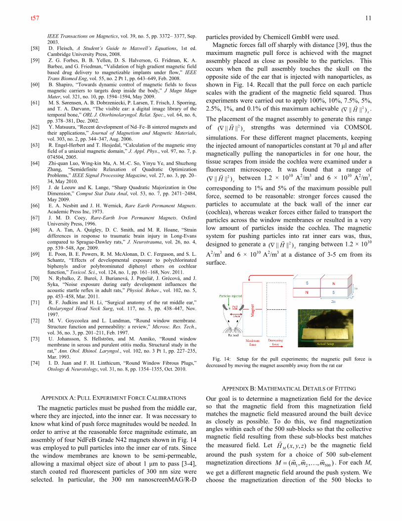
APPENDIX A: PULL EXPERIMENT FORCE CALIBRATIONS

The magnetic particles must be pushed from the middle ear, where they are injected, into the inner ear. It was necessary to know what kind of push force magnitudes would be needed. In order to arrive at the reasonable force magnitude estimate, an assembly of four NdFeB Grade N42 magnets shown in Fig. 14 was employed to pull particles into the inner ear of rats. Since the window membranes are known to be semi-permeable, allowing a maximal object size of about 1 μm to pass [3-4], starch coated red fluorescent particles of 300 nm size were selected. In particular, the 300 nm nanoscreenMAG/R-D

particles provided by Chemicell GmbH were used. Magnetic forces fall off sharply with distance [39], thus the

maximum magnetic pull force is achieved with the magnet assembly placed as close as possible to the particles. This occurs when the pull assembly touches the skull on the opposite side of the ear that is injected with nanoparticles, as shown in Fig. 14. Recall that the pull force on each particle scales with the gradient of the magnetic field squared. Thus experiments were carried out to apply 100%, 10%, 7.5%, 5%, 2.5%, 1%, and 0.1% of this maximum achievable

xH )||||( 2

.

The placement of the magnet assembly to generate this range of

xH )||||( 2

strengths was determined via COMSOL

simulations. For these different magnet placements, keeping the injected amount of nanoparticles constant at 70 μl and after magnetically pulling the nanoparticles in for one hour, the tissue scrapes from inside the cochlea were examined under a fluorescent microscope. It was found that a range of

xH )||||( 2

between 1.2 × 1010 A2/m3 and 6 × 1010 A2/m3,

corresponding to 1% and 5% of the maximum possible pull force, seemed to be reasonable: stronger forces caused the particles to accumulate at the back wall of the inner ear (cochlea), whereas weaker forces either failed to transport the particles across the window membranes or resulted in a very low amount of particles inside the cochlea. The magnetic system for pushing particles into rat inner ears was, thus, designed to generate a

xH )||||( 2

ranging between 1.2 × 1010

A2/m3 and 6 × 1010 A2/m3 at a distance of 3-5 cm from its surface.

Fig. 14: Setup for the pull experiments; the magnetic pull force is decreased by moving the magnet assembly away from the rat ear

APPENDIX B: MATHEMATICAL DETAILS OF FITTING

Our goal is to determine a magnetization field for the device so that the magnetic field from this magnetization field matches the magnetic field measured around the built device as closely as possible. To do this, we find magnetization angles within each of the 500 sub-blocks so that the collective magnetic field resulting from these sub-blocks best matches the measured field. Let ),,( zyxH M

be the magnetic field

around the push system for a choice of 500 sub-element magnetization directions ),,,( 50021 mmmM

. For each M,

we get a different magnetic field around the push system. We choose the magnetization direction of the 500 blocks to

t57

12

minimize the mismatch between ),,( zyxH M

and the

measured magnetic field FH

, meaning, we choose M to

minimize the sum of 2|||| MF HH

across all the

measurement points. Our goal is to choose M only to fit the measured data as best as possible, but the sub-element magnetizations that we find can also be thought of as representing the magnetization anisotropy of the manufactured system.

The magnetic field from each of the sub-blocks can be stated using the analytical expression provided by Herbert and

Hesjedal in [63]. Let ),,( zyxA

, ),,( zyxB

, and ),,( zyxC

represent the analytical expression for the magnetic field around a given rectangular sub-magnet that is uniformly magnetized along the positive x-axis, positive y-axis, and positive z-axis respectively.

Now, let the ith magnet, located at (ai,bi,ci), be uniformly magnetized at an arbitrary angle with respect to the x, y and z-axes. The magnetic field created at location (x,y,z) by this element is

(12) ).,,(),,(

),,(),,(

iiiiiiii

iiiii

czbyaxCczbyaxB

czbyaxAzyxH

The coefficients αi, βi, and γi are the unknown fitting variables. In order to limit the strength of any given element to 1.48 T (which is the remanence magnetization of Grade N52 NdFeB material), the constraint αi

2+ βi2+ γi

2 ≤ 1.482 is imposed for all i = 1,2,3,…,500. For a total number of 500 sub-elements the expression for the collective magnetic field at point j = (x,y,z) is

(13)

).,,(),,(

),,(500

1

iiiiiiii

iiiii

jM

czbyaxCczbyaxB

czbyaxAH

The square of the difference between

FH

, and MH

at point j

can now be written as

(14) 222 ||||22|||||||| jM

jM

jF

jF

jM

jF HHHHHH

.

Define

(15) ),,( iiij

i czbyaxAA

,

(16) ),,( iiij

i czbyaxBB

,

(17) ),,( iiij

i czbyaxCC

.

The term 2|||| j

MH

can be expanded as follows

(18)

jk

jiki

jk

jiki

jk

jiki

jk

jiki

jk

jiki

jk

jiki

jk

jiki

jk

jiki

i k

jk

jiki

jk

jiki

jk

jiki

jM

CCBCACCB

BBABCAAB

CABAAAH

500

1

500

1

2

Define the matrix Q as

jjjjjjjjjjjj

jjjjjjjjjjjj

jjjjjjjjjjjj

jjjjjjjjjjjj

jjjjjjjjjjjj

jjjjjjjjjjjj

j

CCCCBCBCACAC

CCCCBCBCACAC

CBCBBBBBABAB

CBCBBBBBABAB

CACABABAAAAA

CACABABAAAAA

Q

500500150050050015005005001500

500111500111500111

500500150050050015005005001500

500111500111500111

500500150050050015005005001500

50011500111500111 1

:

and define the vector q

as a concatenated list of the modeling

variables αi, βi, and γi as

(19) TTq 500150015001 ,,,,,,,,: .

We can now write, 2|||| j

MH

in compact form as

(20) qQqH jTj

M

2|||| .

The term j

Mj

F HH

can be expanded as follows

(21)

500

1i

jii

jii

jii

jF

jM

jF CBAHHH

(22)

500

1

)()()()(i

yj

Fyj

iij

iij

iixj

Fxj

iij

iij

ii HCBAHCBA

zj

Fzj

iij

iij

ii HCBA )()(

where, for any vector v

, )0,0,1( vv x

,

)0,1,0( vv y

, and )1,0,0( vv z

. Define the vector b

as

(23)

zj

Fzj

Nyj

Fyj

Nxj

Fxj

N

zj

Fzj

yj

Fyj

xj

Fxj

zj

Fzj

Nyj

Fyj

Nxj

Fxj

N

zj

Fzj

yj

Fyj

xj

Fxj

zj

Fzj

Nyj

Fyj

Nxj

Fxj

N

zj

Fzj

yj

Fyj

xj

Fxj

j

HCHCHC

HCHCHC

HBHBHB

HBHBHB

HAHAHA

HAHAHA

b

111

111

111

where N=500. The term j

Mj

F HH

can now be written in

compact form as

(24) jTjM

jF bqHH

.

Note that in (14), 2|||| j

FH

is fixed and cannot be changed as it

is the measured magnetic vector field and, hence, we only need to minimize the expression 2||||2 j

Mj

Mj

F HHH

,

which is equivalent to minimizing qQqbq jTjT 2 for the

measured data point j. In order to minimize the sum of the last expression over all measured data points, define Q to be the

t57

13

sum of all Qj, and b to be the sum of all bj ; our goal is then to minimize qQqbq TT

2 . This expression contains one term

that is linear in q

(i.e., bqT2 ) and another term that is

quadratic in q

(i.e., qQqT ). By introducing a dummy scalar

variable t, we can convert this expression into a pure quadratic form as follows

(25)

q

t

Qb

bqtqQqbqt

TTTT

0

][2 .

Defining

(26) ][ TT qtp

, and

Qb

bQ

T

0~

we can write (25) as pQpqQqbqt TTT ~

2 , with an

additional requirement that the absolute value of t should be

equal to one, i.e. |t| = 1. Note that since pQpT ~ is a quadratic,

replacing p with p

does not change its value. Therefore,

even if the optimization yields t = –1, we can replace p

with

p

making sure that t=1. Requiring that the absolute value of

t to be equal to one is equivalent to requiring t2 = 1. We can further relax this constraint and instead require t2 ≤ 1. Optimization makes use of the extreme values of this bound, i.e. the optimal solution will always generate a value of t = 1, or t = –1. To see this, suppose that jT bq

is negative; picking

any value of t other than –1 will make jT bqt

2 less negative.

Similarly, if jT bq

is positive; picking any value of t other

than 1 will make jT bqt

2 less negative. Thus, the

optimization must pick t = 1, or t = –1, even though other values of t that are in-between these extreme values are allowed. In order to write this constraint in matrix form, let G1 be a 3(N+1)×3(N+1) matrix (with N=500) with having 1 at the location (1,1) and zeros everywhere else; this constraint can then be written in matrix form as

(27) 11 pGpT

To include the αi

2+ βi2+ γi

2 ≤ 1.482 magnetization constraints, let Gi+1 be a )1(3)1(3 NN matrix having 1/(1.482) at the

locations )1,1( ii , )1,1( iNiN , and )12,12( iNiN

and zeros everywhere else. Then the element magnetization constraints can be written in matrix form as

(28) 11 pGp iT

.

The fitting problem, therefore, can be stated as follows: minimize the cost pQpT ~ subject to the constraint of equation

(27) and the N (=500) constraints of equation (28), one for each element (for i = 1, 2, … 500 sub-magnets). We, therefore have a quadratic cost to minimize, along with quadratic constraints. We employ a combination of two methods to find the optimal solutions: 1) semi-definite

relaxation [64] and 2) the majorization method [65]. Further details on the technique we employ to solve this type of problem can be found in [19].

ACKNOWLEDGEMENT

This research was supported in part by funding from the National Institutes of Health (NIH).