Embed Size (px)
Citation preview
Magnetic fields and tokamak plasmas Alan Wootton
1
Magnetic Fields and Magnetic Diagnostics
for
Tokamak Plasmas
Alan Wootton
pitch changes sign 'width' changes sign
p pII
Magnetic fields and tokamak plasmas Alan Wootton
2
INTRODUCTION........................................................................................................................... 5
1. SOME CONCEPTS AND DEFINITIONS................................................................................ 7
Maxwell's equations.................................................................................................................... 7
Pick-up or Induction Coils .......................................................................................................... 7
Integration ................................................................................................................................... 8
Vector potential......................................................................................................................... 12
Mutual inductance..................................................................................................................... 16
Self inductance.......................................................................................................................... 17
Poloidal flux.............................................................................................................................. 18
Field lines and flux surfaces ..................................................................................................... 21
An example ............................................................................................................................... 23
Circuit equations ....................................................................................................................... 28
2. SOME NON STANDARD MEASUREMENT TECHNIQUES............................................. 30
Hall Probe ................................................................................................................................. 30
Faraday Effect ........................................................................................................................... 31
The Compass............................................................................................................................. 31
Flux gates .................................................................................................................................. 32
3. GENERAL FIELD CHARACTERIZATION.......................................................................... 34
Fourier components .................................................................................................................. 34
Field components on a rectangle............................................................................................... 36
4. PLASMA CURRENT.............................................................................................................. 39
Rogowski coil ........................................................................................................................... 39
5. LOOP VOLTS, VOLTS per TURN, SURFACE VOLTAGE.............................................. 40
Introduction............................................................................................................................... 40
The single volts per turn loop ................................................................................................... 40
Poynting’s theorem ................................................................................................................... 41
Uses of the Volts per turn measurement ................................................................................... 44
6. TOKAMAK EQUILIBRIA....................................................................................................... 45
6.0. AN INTUITIVE DERIVATION OF TOKAMAK EQUILIBRIUM ................................ 45
Introduction........................................................................................................................... 45
Energy associated with plasma pressure ............................................................................... 46
Energy associated with toroidal fields .................................................................................. 47
Energy associated with poloidal fields.................................................................................. 48
Total forces ........................................................................................................................... 49
6.1. THE FLUX OUTSIDE A CIRCULAR TOKAMAK ........................................................ 50
6. CIRCULAR EQUILIBRIUM .............................................................................................. 53
Derivation of the Grad Shafranov equation .......................................................................... 53
Solving the Grad Shafranov equation ................................................................................... 57
The poloidal field at the plasma edge ................................................................................... 59
Simple current distributions.................................................................................................. 60
The surface displacements: the Shafranov Shift ................................................................... 64
Matching vacuum and plasma solutions ............................................................................... 65
More complicated configurations. ........................................................................................ 69
7. Position and βI + li/2 for the circular equilibrium ................................................................... 70
Magnetic fields and tokamak plasmas Alan Wootton
3
An ‘exact’ circular equilibrium................................................................................................. 70
Extension of position measurement to non circular shapes ...................................................... 73
Extension of βI + li/2 measurement to non circular shapes...................................................... 74
Non-circular contours. .............................................................................................................. 75
8. SOME FUNDAMENTAL RELATIONS ................................................................................ 78
Geometry................................................................................................................................... 78
Field representation................................................................................................................... 79
Identities.................................................................................................................................... 80
Ideal MHD ................................................................................................................................ 82
Boundary conditions ................................................................................................................. 82
9. MOMENTS OF THE TOROIDAL CURRENT DENSITY.................................................... 84
10. PLASMA POSITION ............................................................................................................ 87
Position by multipole moments ................................................................................................ 87
Application to the large aspect ratio circular tokamak.............................................................. 89
11. PLASMA SHAPE.................................................................................................................. 92
12. MOMENTS OF PLASMA PRESSURE ............................................................................... 94
The Virial Equation................................................................................................................... 94
m = -1, B2 = Bext ..................................................................................................................... 96
m = 0, B2 = 0 ............................................................................................................................ 97
m = -1, B2 = 0 ........................................................................................................................... 98
13. βI + li/2 ................................................................................................................................ 100
Solution................................................................................................................................... 100
Separation of βI and li............................................................................................................. 101
Comments on the definition of poloidal beta.......................................................................... 102
14. DIAMAGNETISM .............................................................................................................. 103
Comments ............................................................................................................................... 103
Microscopic picture for a square profile plasma in a cylinder................................................ 103
Macroscopic picture................................................................................................................ 104
Paramagnetic and diamagnetic flux ........................................................................................ 105
Toroidal, non circular geometry.............................................................................................. 106
The meaning of βI................................................................................................................... 107
Measurements ......................................................................................................................... 109
15. FULL EQUILIBRIUM RECONSTRUCTION.................................................................... 113
16. FAST SURFACE RECONSTRUCTION............................................................................ 115
17. FLUCTUATING FIELDS ................................................................................................... 118
(MIRNOV OSCILLATIONS and TURBULENCE) .................................................................. 118
Mirnov Oscillations ................................................................................................................ 118
Analysis techniques................................................................................................................. 124
Turbulence .............................................................................................................................. 127
18. INTERNAL PLASMA MEASUREMENTS....................................................................... 133
Equilibrium ............................................................................................................................. 134
Mirnov Oscillations ................................................................................................................ 138
19 . THE CONDUCTING VACUUM VESSEL....................................................................... 140
Skin depths.............................................................................................................................. 140
Application to a diamagnetic loop .......................................................................................... 142
Magnetic fields and tokamak plasmas Alan Wootton
4
Application to position measurement ..................................................................................... 143
20 . THE IRON CORE .............................................................................................................. 144
21. TOKAMAK POSITION CONTROL .................................................................................. 149
The axisymmetric instability................................................................................................... 149
Analysis of sensor coils allowing for vessel currents ............................................................. 152
The dipole model .................................................................................................................... 152
The feedback model ................................................................................................................ 156
Application of stability criteria. .............................................................................................. 159
22. MAGNETIC ISLANDS........................................................................................................ 161
23. SOME EXPERIMENTAL TECHNIQUES.......................................................................... 164
Coils winding.......................................................................................................................... 164
Interference suppression.......................................................................................................... 164
Screened rooms....................................................................................................................... 165
Misaligned sensor coils........................................................................................................... 166
Magnetic fields and tokamak plasmas Alan Wootton
5
INTRODUCTION
This series of notes tries to lay the foundations for the interpretation of magnetic fields and
fluxes, often in terms of equilibrium plasma parameters. The title, 'magnetic diagnostics', is
taken to mean those diagnostics which are used to measure magnetic fields and fluxes using
induction, or pick-up, coils. More specifically, what is often inferred is a question: "How much
can we tell about a plasma given certain measurements of magnetic fields, and fluxes, outside
that plasma?" I don’t consider here diagnostics which measure the plasma current density
distribution utilizing phenomena such as the motional Stark effect, or Faraday rotation; these are
found in a series of notes on Plasma Diagnostics..
The measurements themselves are in principle simple, although in practice they are always
complicated by unwanted field components, for example from misaligned pick-up coils. There is
also the problem of allowing for image currents flowing in nearby conductors; dealing with these
image currents becomes a large part of the problem. Including the effects of an iron core also
leads to complications.
Many people think the topic under consideration is boring, in that there is nothing new to do.
You have only to read current issues of plasma physics journals to recognize that there is still
much interest in the topic. For example, equilibrium and its determination, axisymmetric stability
and disruptions are all of current interest, and all involve ‘magnetic diagnostics’. The subject
does appear to be difficult (students starting in the topic have a hard time).
The layout of the notes is as given in the list of contents. Generally I have included topics which
I have found useful in trying to understand tokamaks. Some basic concepts (inductances, fluxes,
etc.) are included, because they are made use of throughout the notes. There is also a section on
plasma equilibrium, in which the large aspect ratio, circular tokamak is described. The fluxes
and fields from this model are used as examples for application of certain ideas in the remainder
of the text.
References I find useful include:
o B. J. Braams, The interpretation of tokamak diagnostics: status and prospects, IPP
Garching report IPP 5/2, 1985.
o L. E. Zakharov and V. D. Shafranov, Equilibrium of current carrying plasmas in toroidal
configurations, in Reviews of Plasma Physics volume 11, edited by M. A.
Leontovich, Consultants Bureau, New York (1986).
o V. S. Mukhovatov and V. D. Shafranov, Nucl. Fusion 11 (1971) 605.
o V. D. Shafranov, Plasma Physics 13 (1971) 757.
o L. E. Zakharov and V. D. Shafranov, Sov. Phys. Tech. Phys. 18 (1973) 151

Magnetic fields and tokamak plasmas Alan Wootton
6
o J. A. Wesson, in Tokamaks, Oxford Science Publications, Clarendon press, Oxford, 1987.
o P. Shkarofsky, Evaluation of multipole moments over the current density in a tokamak
with magnetic probes, Phys. Fluids 25 (1982) 89.
Magnetic fields and tokamak plasmas Alan Wootton
7
1. SOME CONCEPTS AND DEFINITIONS
Maxwell's equations
We are going to make extensive use of Maxwell’s equations. In vector form, these are
∇ × B = µ j +∂D
∂t
1.1
∇ ⋅ B = 0 1.2
∇ × E = −∂B
∂t 1.3
∇ ⋅ D = ρ 1.4
If charge is conserved we can add to these the continuity equation. We shall ignore the
displacement current ∂D/∂t, and take µ = µo, the free space value, inside a plasma. Without the
last term Equation 1.1 is Amperes law. We have effectively restricted ourselves to assuming ni =
ne = n, the charge neutral assumption, and that any waves have frequencies much less than the
electron plasma frequency, with characteristic lengths much greater than the Debye length . We
have not said E or ∇.E = 0. When considering plasma equilibrium we shall also assume the
electron mass me approaches 0. This allows electrons to have an infinitely fast response time.
Pick-up or Induction Coils
This is the heart of the matter. Magnetic fields are usually measured with pick-up or induction
coil circuits. Changing the magnetic flux in a circuit generates a current; the direction of this
current is in a direction such as to set up a magnetic flux opposing the change. The
electromotence or voltage ε (∇ ε = -E, the electric field intensity) in Volts induced in a circuit
equals the rate of change of flux N = B ⋅ ndSS∫ in Webers per second, i.e.
ε =dN
dt 1.5
The flux can be changed either by changing its strength, changing the shape of the circuit, or
moving the circuit. Then
E ⋅ dll∫ = −
d
dtB ⋅ndS
S∫ 1.6
Magnetic fields and tokamak plasmas Alan Wootton
8
for any path l, with n the normal to a two sided surface S. Applying Stokes theorem
( A • dl =l∫ n • ∇ × AdS
S
∫ for any vector A) to the left hand side of Equation 1.6 gives Equation
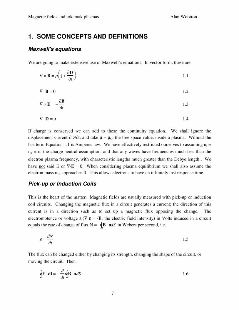
1.3. Figure 1.1 shows the geometry of a coil used in applying Equation 1.6, Faraday’s Law. The
output signal must be time integrated to obtain the required flux. By taking a small enough coil
the local field B can then be determined. This becomes difficult if very small scale variations in
field exist, because the pick-up coils must then be very small themselves. The surface S includes
any area between the leads; this is minimized by twisting them together. A hand drill is
particularly useful for this.
Surface S
Contour l
Coil
leads
voltage producedacross leads
Figure 1.1. The contour l and surface S of a pick-up coil.
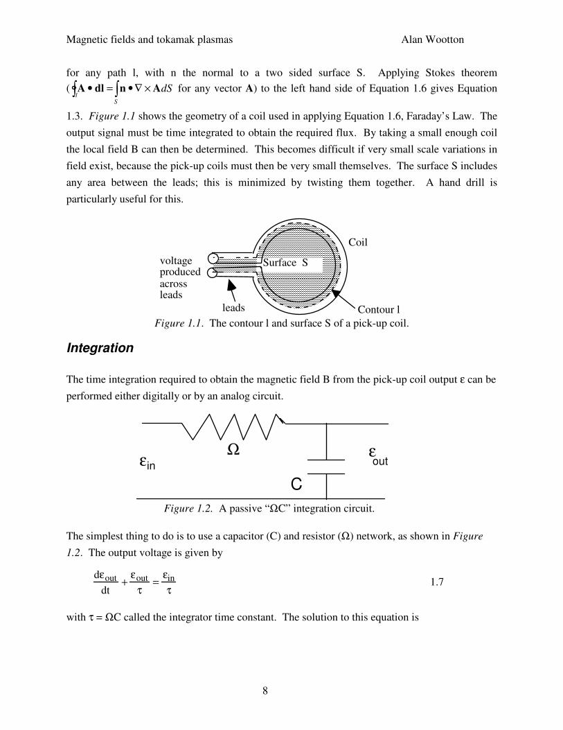
Integration
The time integration required to obtain the magnetic field B from the pick-up coil output ε can be
performed either digitally or by an analog circuit.
εinεout
Ω
C
Figure 1.2. A passive “ΩC” integration circuit.
The simplest thing to do is to use a capacitor (C) and resistor (Ω) network, as shown in Figure
1.2. The output voltage is given by
dεout
dt+
εout
τ=
εin
τ 1.7
with τ = ΩC called the integrator time constant. The solution to this equation is
Magnetic fields and tokamak plasmas Alan Wootton
9
εout = e− t
τ e−t'
τ
εin (t
')
dt'
τ0
t
∫ 1.8
For example, suppose at t = 0 we start an input voltage εin = εin0 sin(ωt), so that the required
integral is εint = εin0 (1-cos(ωt))/ω. The output from the passive circuit is (obtained using
Laplace transforms)
εout = εin0ωτ
etτ 1 + ωτ( )2( )
+sin(ωt) − ωτ cos(ωt)
1 + ωτ( )2( )
1.9
Now consider two extremes. First, if ωτ >> 1 and t << τ we have
εout =εin0
ωτ1− cos(ωt)( ) 1.10
That is, εout = 1/τ times the required integral. In this limit we have integrated the input signal. If
ωτ << 1 and t >> τ, then εout = εin.
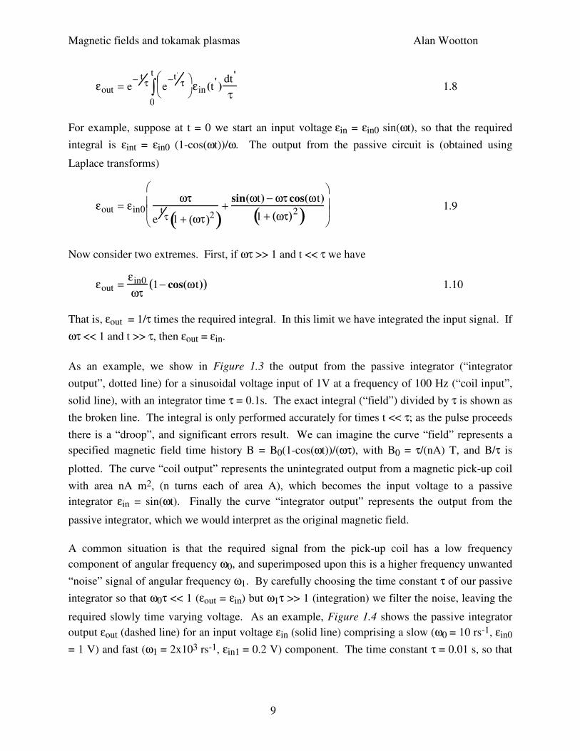
As an example, we show in Figure 1.3 the output from the passive integrator (“integrator
output”, dotted line) for a sinusoidal voltage input of 1V at a frequency of 100 Hz (“coil input”,
solid line), with an integrator time τ = 0.1s. The exact integral (“field”) divided by τ is shown as
the broken line. The integral is only performed accurately for times t << τ; as the pulse proceeds
there is a “droop”, and significant errors result. We can imagine the curve “field” represents a
specified magnetic field time history B = B0(1-cos(ωt))/(ωτ), with B0 = τ/(nA) T, and B/τ is
plotted. The curve “coil output” represents the unintegrated output from a magnetic pick-up coil
with area nA m2, (n turns each of area A), which becomes the input voltage to a passive
integrator εin = sin(ωt). Finally the curve “integrator output” represents the output from the
passive integrator, which we would interpret as the original magnetic field.
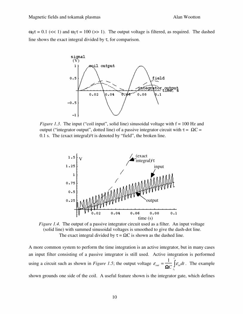
A common situation is that the required signal from the pick-up coil has a low frequency
component of angular frequency ω0, and superimposed upon this is a higher frequency unwanted
“noise” signal of angular frequency ω1. By carefully choosing the time constant τ of our passive
integrator so that ω0τ << 1 (εout = εin) but ω1τ >> 1 (integration) we filter the noise, leaving the
required slowly time varying voltage. As an example, Figure 1.4 shows the passive integrator
output εout (dashed line) for an input voltage εin (solid line) comprising a slow (ω0 = 10 rs-1, εin0
= 1 V) and fast (ω1 = 2x10³ rs-1, εin1 = 0.2 V) component. The time constant τ = 0.01 s, so that
Magnetic fields and tokamak plasmas Alan Wootton
10
ω0τ = 0.1 (<< 1) and ω1τ = 100 (>> 1). The output voltage is filtered, as required. The dashed
line shows the exact integral divided by τ, for comparison.
(V)
Figure 1.3. The input (“coil input”, solid line) sinusoidal voltage with f = 100 Hz and
output (“integrator output”, dotted line) of a passive integrator circuit with τ = ΩC =
0.1 s. The (exact integral)/τ is denoted by “field”, the broken line.
time (s)
input
(exact integral)/τ
output
V
Figure 1.4. The output of a passive integrator circuit used as a filter. An input voltage
(solid line) with summed sinusoidal voltages is smoothed to give the dash-dot line.
The exact integral divided by τ = ΩC is shown as the dashed line.
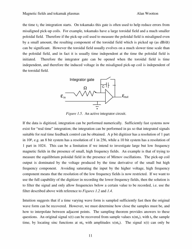
A more common system to perform the time integration is an active integrator, but in many cases
an input filter consisting of a passive integrator is still used. Active integration is performed
using a circuit such as shown in Figure 1.5; the output voltage εout =1
ΩΩΩΩCε indt
t1
t
∫ . The example
shown grounds one side of the coil. A useful feature shown is the integrator gate, which defines
Magnetic fields and tokamak plasmas Alan Wootton
11
the time t1 the integration starts. On tokamaks this gate is often used to help reduce errors from
misaligned pick-up coils. For example, tokamaks have a large toroidal field and a much smaller
poloidal field. Therefore if the pick-up coil used to measure the poloidal field is misaligned even
by a small amount, the resulting component of the toroidal field which is picked up (as dB/dt)
can be significant. However the toroidal field usually evolves on a much slower time scale than
the poloidal field, and in fact it is usually time independent at the time the poloidal field is
initiated. Therefore the integrator gate can be opened when the toroidal field is time
independent, and therefore the induced voltage in the misaligned pick-up coil is independent of
the toroidal field.
Integrator gate
inε εout
Ω C
.
Figure 1.5. An active integrator circuit.
If the data is digitized, integration can be performed numerically. Sufficiently fast systems now
exist for “real time” integration; the integration can be performed in µs so that integrated signals
suitable for real time feedback control can be obtained. A p bit digitizer has a resolution of 1 part
in 10p, e.g. an 8 bit system has a resolution of 1 in 256, while a 10 bit system has a resolution of
1 part in 1024. This can be a limitation if we intend to investigate large but low frequency
magnetic fields in the presence of small, high frequency fields. An example is that of trying to
measure the equilibrium poloidal field in the presence of Mirnov oscillations. The pick-up coil
output is dominated by the voltage produced by the time derivative of the small but high
frequency component. Avoiding saturating the input by the higher voltage, high frequency
component means that the resolution of the low frequency fields is now restricted. If we want to
use the full capability of the digitizer in recording the lower frequency fields, then the solution is
to filter the signal and only allow frequencies below a certain value to be recorded, i.e. use the
filter described above with reference to Figures 1.2 and 1.4.
Intuition suggests that if a time varying wave form is sampled sufficiently fast then the original
wave form can be recovered. However, we must determine how close the samples must be, and
how to interpolate between adjacent points. The sampling theorem provides answers to these
questions. An original signal x(t) can be recovered from sample values x(nts), with ts the sample
time, by locating sinc functions at nts with amplitudes x(nts). The signal x(t) can only be
Magnetic fields and tokamak plasmas Alan Wootton
12
recovered if the signal bandwidth b ≤ fs/2, with fs the sampling frequency = 1/ts. If this is not
done, aliasing occurs.
If b > fs/2 then the high frequency signal can appear as a low frequency signal. The fact that
spoked wheels in films sometimes appear to rotate backwards is a manifestation of aliasing.
Aliasing can be avoided using a passive filter to remove the high frequencies f > fs/2. For
example, sampling at 5 kHz (i.e. a sample every 0.2 ms) then an “anti aliasing” filter with τ = 0.5
ms can be used.
Vector potential
In describing plasma equilibria we shall make use of the vector potential A. It is related to the
poloidal flux, and used to determine self and mutual inductances. It is defined through the
equation
∇ × A = B 1.11
In cylindrical geometry (R,φ,z), which we shall use a lot, this is
BR =1
R
∂Az
∂φ−
∂Aφ
∂z
Bφ =∂AR
∂z−
∂Az
∂R
Bz = 1
R
∂ RAφ( )∂R
− 1
R
∂AR
∂φ
1.12
Then the electric intensity E is proportional to the vector potential A whose change produces it:
E = −dA
dt 1.13
From Equation 1.1 (ignoring D and ρ) we then have that A is given in terms of the current
density j (the current per unit area) by Poisson's equation:
∇2A = −µj 1.14
which has a solution
A =µ
4πjdV
rV∫ =µ
4πIdl
r∫ 1.15
Magnetic fields and tokamak plasmas Alan Wootton
13
where the total current I flows inside the volume V, the line element dl is along the direction of
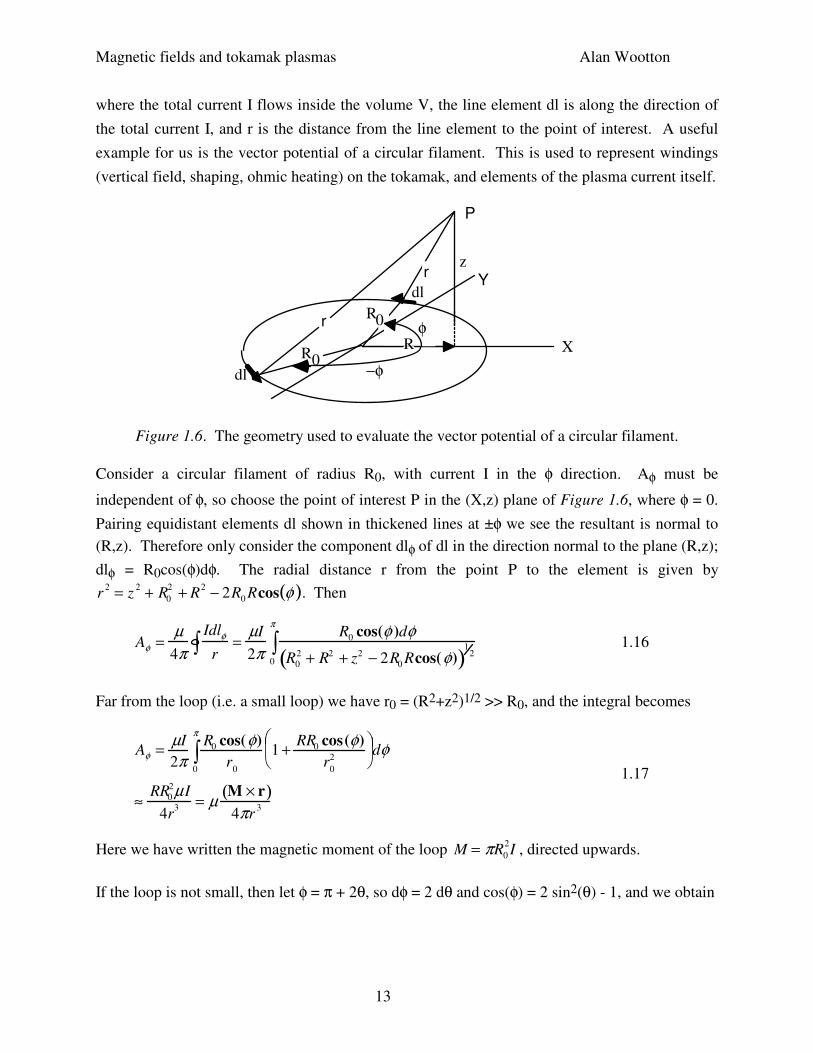
the total current I, and r is the distance from the line element to the point of interest. A useful
example for us is the vector potential of a circular filament. This is used to represent windings
(vertical field, shaping, ohmic heating) on the tokamak, and elements of the plasma current itself.
P
Y
X
r
r
dl
dl
R0R
φ
z
R0
−φ
Figure 1.6. The geometry used to evaluate the vector potential of a circular filament.
Consider a circular filament of radius R0, with current I in the φ direction. Aφ must be
independent of φ, so choose the point of interest P in the (X,z) plane of Figure 1.6, where φ = 0.
Pairing equidistant elements dl shown in thickened lines at ±φ we see the resultant is normal to
(R,z). Therefore only consider the component dlφ of dl in the direction normal to the plane (R,z);
dlφ = R0cos(φ)dφ. The radial distance r from the point P to the element is given by
r2 = z
2 + R0
2 + R2 − 2R0 Rcos φ( ). Then
Aφ =µ
4πIdlφ
r∫ =µI
2πR0 cos(φ )dφ
R0
2 + R2 + z2 − 2R0 Rcos(φ)( )1
20
π
∫ 1.16
Far from the loop (i.e. a small loop) we have r0 = (R2+z2)1/2 >> R0, and the integral becomes
Aφ =µI
2πR0 cos(φ)
r0
1 +RR0 cos(φ)
r0
2
0
π
∫ dφ
≈RR0
2µI
4r3 = µ
M × r( )4πr
3
1.17
Here we have written the magnetic moment of the loop M = πR0
2I , directed upwards.
If the loop is not small, then let φ = π + 2θ, so dφ = 2 dθ and cos(φ) = 2 sin2(θ) - 1, and we obtain
Magnetic fields and tokamak plasmas Alan Wootton
14
Aφ =µR0 I
π
2sin2 (θ) −1( )dθ
R0 + R( )2 + z 2 − 4R0R sin2 (θ)( )1
20
π2
∫ 1.18
This can be re-written in terms of K(k2) and E(k2), the complete elliptic integrals of the first and
second kind, ( E m( ) = 1− msin2 θ( )( )
0
π2
∫ dθ , K m( ) =dθ
1− m sin2 θ( )( )0
π2
∫ as
AΦ = µI
πk
R0
R
12
1 − k2
2
K − E
k2 = 4R0R R0 + R( )2
+ z2[ ]−1
1.19
φ
R
Z
ρ
ω
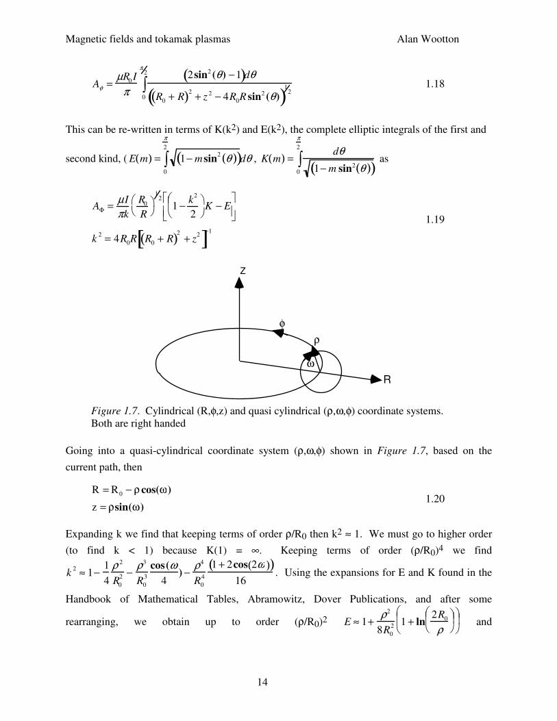
Figure 1.7. Cylindrical (R,φ,z) and quasi cylindrical (ρ,ω,φ) coordinate systems.
Both are right handed
Going into a quasi-cylindrical coordinate system (ρ,ω,φ) shown in Figure 1.7, based on the
current path, then
R = R0 − ρcos(ω)
z = ρsin(ω) 1.20
Expanding k we find that keeping terms of order ρ/R0 then k2 ≈ 1. We must go to higher order
(to find k < 1) because K(1) = ∞. Keeping terms of order (ρ/R0)4 we find
k2 ≈ 1−
1
4
ρ 2
R0
2 −ρ3
R0
3
cos(ω4
) −ρ4
R0
4
1 + 2cos 2ω( )( )16
. Using the expansions for E and K found in the
Handbook of Mathematical Tables, Abramowitz, Dover Publications, and after some
rearranging, we obtain up to order (ρ/R0)2 E ≈ 1+ρ2
8R0
2 1 + ln2R0
ρ
and
Magnetic fields and tokamak plasmas Alan Wootton
15
K ≈ ln8R0
ρ
−
ρ2R0
cos ω( ) +ρ2
16R0
2 ln2R0
ρ
+
1
21 + 4cos 2ω( )( )
. Finally we can write an
expression for the vector potential near the loop keeping terms of order (ρ/R0):
Aφ ≈µ 0 I
2πln
8R0
ρ
− 2
+
ρR0
cos ω( )2
ln8R0
ρ
− 3
1.21
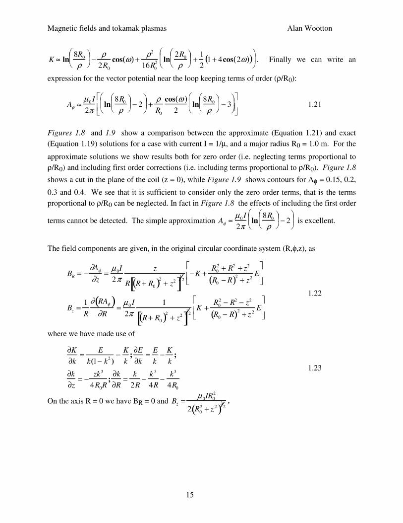
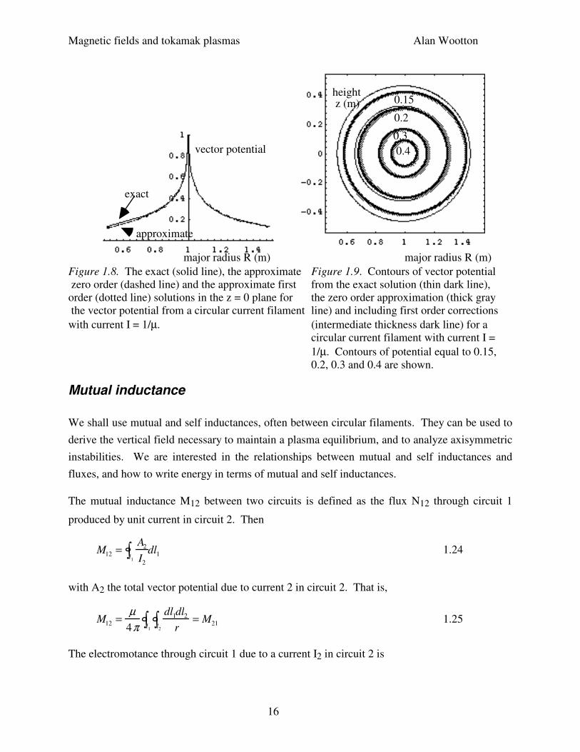
Figures 1.8 and 1.9 show a comparison between the approximate (Equation 1.21) and exact
(Equation 1.19) solutions for a case with current I = 1/µ, and a major radius R0 = 1.0 m. For the
approximate solutions we show results both for zero order (i.e. neglecting terms proportional to
ρ/R0) and including first order corrections (i.e. including terms proportional to ρ/R0). Figure 1.8
shows a cut in the plane of the coil (z = 0), while Figure 1.9 shows contours for Aφ = 0.15, 0.2,
0.3 and 0.4. We see that it is sufficient to consider only the zero order terms, that is the terms
proportional to ρ/R0 can be neglected. In fact in Figure 1.8 the effects of including the first order
terms cannot be detected. The simple approximation Aφ ≈µ 0 I
2πln
8R0
ρ
− 2
is excellent.
The field components are given, in the original circular coordinate system (R,φ,z), as
BR = −∂Aφ
∂z=
µ 0I
2πz
R R + R0( )2
+ z2[ ]1
2
−K +R0
2 + R2 + z2
R0 − R( )2 + z2E
Bz =1
R
∂ RAφ( )∂R
=µ 0 I
2π1
R + R0( )2
+ z2[ ]1
2K +
R0
2 − R2 − z2
R0 − R( )2 + z 2E
1.22
where we have made use of
∂K
∂k=
E
k(1− k2)
−K
k;
∂E
∂k=
E
k−
K
k;
∂k
∂z= −
zk3
4R0R;
∂k
∂R=
k
2R−
k 3
4R−
k3
4R0
1.23
On the axis R = 0 we have BR = 0 and Bz =µ0IR0
2
2 R0
2 + z 2( )3
2.
Magnetic fields and tokamak plasmas Alan Wootton
16
major radius R (m)
exact
approximate
vector potential
height z (m)
major radius R (m)
0.4
0.3
0.15
0.2
Figure 1.8. The exact (solid line), the approximate Figure 1.9. Contours of vector potential
zero order (dashed line) and the approximate first from the exact solution (thin dark line),
order (dotted line) solutions in the z = 0 plane for the zero order approximation (thick gray
the vector potential from a circular current filament line) and including first order corrections
with current I = 1/µ. (intermediate thickness dark line) for a
circular current filament with current I =
1/µ. Contours of potential equal to 0.15,
0.2, 0.3 and 0.4 are shown.
Mutual inductance
We shall use mutual and self inductances, often between circular filaments. They can be used to
derive the vertical field necessary to maintain a plasma equilibrium, and to analyze axisymmetric
instabilities. We are interested in the relationships between mutual and self inductances and
fluxes, and how to write energy in terms of mutual and self inductances.
The mutual inductance M12 between two circuits is defined as the flux N12 through circuit 1
produced by unit current in circuit 2. Then
M12 =A2
I2l1∫ dl1 1.24
with A2 the total vector potential due to current 2 in circuit 2. That is,
M12 =µ
4πdl1dl2
rl2∫l1
∫ = M21 1.25
The electromotance through circuit 1 due to a current I2 in circuit 2 is
Magnetic fields and tokamak plasmas Alan Wootton
17
ε1 = M12
dI2
dt 1.26
The total energy (in a volume V) associated with two circuits is
Wt =1
2µB1 + B2( )
V∫ • B1 + B2( )dV
=1
2µB1
2
V∫ dV +1
2µB2
2
V∫ dV +1
µB1 • B2V∫ dV
1.27
The first two terms represent the energy required to establish the currents I1 and I2 producing the
fields B1 and B2 in circuits 1 and 2. The third term is the energy used in bringing the two circuits
together. This mutual energy between the two circuits W12 is
W12 = M12I1I2 =1
µB1B2dV
V∫ 1.28
Self inductance
The magnetic energy density W of a single circuit carrying current I1 is used to define the self
inductance L11 of the circuit:
W =1
2µB
2
V∫ dV =1
2L11I1
2 1.29
To maintain the current I1 a power source must, in each second, do an amount of work
ε1I1 = I1
dN1
dt 1.30
(because ε = dN/dt) in addition to working against resistance Ω. The stored energy per second in
the magnetic field equals dW/dt, so that
I1
dN1
dt= L11I1
dI1
dt 1.31
i.e.
N11 = L11I1 1.32
Therefore we can also define the self inductance of a circuit through the change in flux linking
that circuit when the current changes by one unit:
Magnetic fields and tokamak plasmas Alan Wootton
18
ε1 =dN11
dt= L11
dI1
dt 1.33
Poloidal flux
Suppose that a system consists only of toroidally wound loops producing only poloidal fields. In
a cylindrical coordinate system R,φ,z shown in Figure 1.7 (φ is also the ‘toroidal' angle in a quasi
cylindrical coordinate system) nothing depends on the angle φ. Then
M12 = 2πR1
A2
I2
1.34
and A has only a toroidal component Aφ. In this case the fields are given by (B =∇xA):
BR = −∂Aφ
∂z
Bφ = 0
Bz = 1
R
∂ RAφ( )∂R
1.35
These poloidal fields are also expressed in terms of the transverse (poloidal) flux function
Ψ: Ψ(R,z) = constant defines the form of the equilibrium magnetic surfaces, proved later:
B =1
2πR∇ΨΨΨΨ × eφ( ) 1.36
with eφ a unit vector in the toroidal (φ) direction, so that
Bz =1
2πR
∂ΨΨΨΨ∂R
BR = −1
2πR
∂ΨΨΨΨ∂z
1.37
But we know that we can write, in terms of the vector potential for our toroidally symmetric
system (∂/∂φ = 0),
BR = −∂Aφ
∂z
Bz =1
R
∂ RAφ( )∂R
1.38
That is, the poloidal flux can be written as (with subscripts implied but not given):
Magnetic fields and tokamak plasmas Alan Wootton
19
ΨΨΨΨ = 2πRAφ = MI = 2π Bz RdR0
R
∫ 1.39
That is, for the system we are considering, the poloidal flux at a position R is simply the vertical
field Bz integrated across a circle of radius R. Note that sometimes in the literature the flux
function ψ = Ψ/(2π) is used.
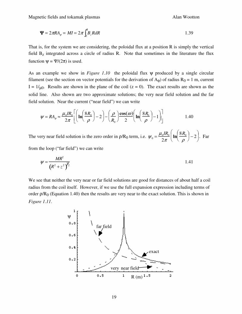
As an example we show in Figure 1.10 the poloidal flux ψ produced by a single circular
filament (see the section on vector potentials for the derivation of Aφ) of radius R0 = 1 m, current
I = 1/µ0. Results are shown in the plane of the coil (z = 0). The exact results are shown as the
solid line. Also shown are two approximate solutions; the very near field solution and the far
field solution. Near the current (“near field”) we can write
ψ = RAφ ≈µ 0IR0
2πln
8R0
ρ
− 2
−
ρR0
cos ω( )
2ln
8R0
ρ
−1
1.40
The very near field solution is the zero order in ρ/R0 term, i.e. ψ 0 =µ0IR0
2πln
8R0
ρ
− 2
. Far
from the loop (“far field”) we can write
ψ =MR2
R2 + z 2( )3
2 1.41
We see that neither the very near or far field solutions are good for distances of about half a coil
radius from the coil itself. However, if we use the full expansion expression including terms of
order ρ/R0 (Equation 1.40) then the results are very near to the exact solution. This is shown in
Figure 1.11.
ψ
exact
far field
near field
R (m)
very
Magnetic fields and tokamak plasmas Alan Wootton
20
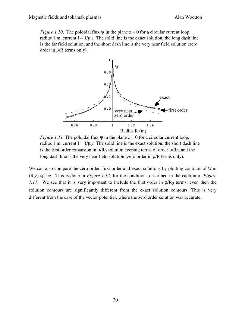
Figure 1.10. The poloidal flux ψ in the plane z = 0 for a circular current loop,
radius 1 m, current I = 1/µ0. The solid line is the exact solution, the long dash line
is the far field solution, and the short dash line is the very near field solution (zero
order in ρ/R terms only).
ψ
Radius R (m)
exact
very near first orderzero order
Figure 1.11 The poloidal flux ψ in the plane z = 0 for a circular current loop,
radius 1 m, current I = 1/µ0. The solid line is the exact solution, the short dash line
is the first order expansion in ρ/R0 solution keeping terms of order ρ/R0, and the
long dash line is the very near field solution (zero order in ρ/R terms only).
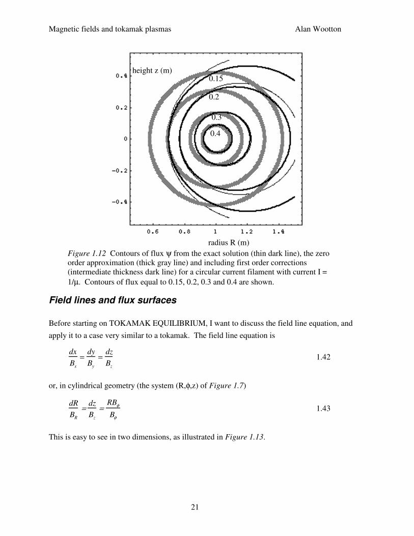
We can also compare the zero order, first order and exact solutions by plotting contours of ψ in
(R,z) space. This is done in Figure 1.12, for the conditions described in the caption of Figure
1.11. We see that it is very important to include the first order in ρ/R0 terms; even then the
solution contours are significantly different from the exact solution contours. This is very
different from the case of the vector potential, where the zero order solution was accurate.
Magnetic fields and tokamak plasmas Alan Wootton
21
height z (m)
radius R (m)
0.4
0.3
0.2
0.15
Figure 1.12 Contours of flux ψ from the exact solution (thin dark line), the zero
order approximation (thick gray line) and including first order corrections
(intermediate thickness dark line) for a circular current filament with current I =
1/µ. Contours of flux equal to 0.15, 0.2, 0.3 and 0.4 are shown.
Field lines and flux surfaces
Before starting on TOKAMAK EQUILIBRIUM, I want to discuss the field line equation, and
apply it to a case very similar to a tokamak. The field line equation is
dx
Bx
=dy
By
=dz
Bz
1.42
or, in cylindrical geometry (the system (R,φ,z) of Figure 1.7)
dR
BR
=dz
Bz
=RBφ
Bφ
1.43
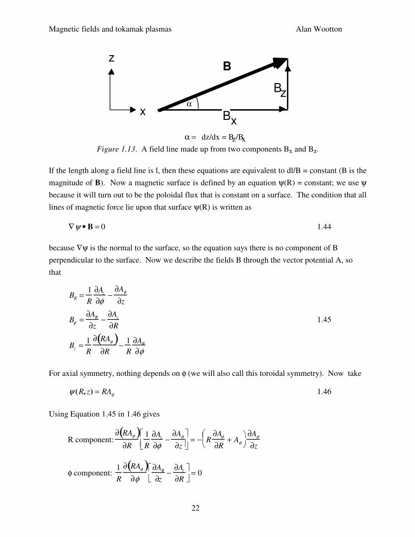
This is easy to see in two dimensions, as illustrated in Figure 1.13.
Magnetic fields and tokamak plasmas Alan Wootton
22
B
B
B
z
x
z
x α
α = dz/dx = B /Bz x Figure 1.13. A field line made up from two components Bx and Bz.
If the length along a field line is l, then these equations are equivalent to dl/B = constant (B is the
magnitude of B). Now a magnetic surface is defined by an equation ψ(R) = constant; we use ψ
because it will turn out to be the poloidal flux that is constant on a surface. The condition that all
lines of magnetic force lie upon that surface ψ(R) is written as
∇ψ • B = 0 1.44
because ∇ψ is the normal to the surface, so the equation says there is no component of B
perpendicular to the surface. Now we describe the fields B through the vector potential A, so
that
BR =1
R
∂Az
∂φ−
∂Aφ
∂z
Bφ =∂AR
∂z−
∂Az
∂R
Bz = 1
R
∂ RAφ( )∂R
− 1
R
∂AR
∂φ
1.45
For axial symmetry, nothing depends on φ (we will also call this toroidal symmetry). Now take
ψ (R, z) = RAφ 1.46
Using Equation 1.45 in 1.46 gives
R component:∂ RAφ( )
∂R
1
R
∂Az
∂φ−
∂Aφ
∂z
= − R
∂Aφ
∂R+ Aφ
∂Aφ
∂z
φ component: 1
R
∂ RAφ( )∂φ
∂AR
∂z−
∂Az
∂R
= 0
Magnetic fields and tokamak plasmas Alan Wootton
23
z component : ∂ RAφ( )
∂z
1
R
∂ RAφ( )∂R
−1
R
∂AR
∂φ
=
∂Aφ
∂zR
∂Aφ
∂R+ Aφ
1.47
where the RHS of each equation represents the result for ∂/∂φ = 0. Therefore, with the assumed
symmetry, the φ component is zero and the R component and z component cancel. Therefore our
assumed form for the surface (Equation 1.46, ψ (R, z) = RAφ ) ensures that ∇ψ • B = 0 , i.e. it
ensures that all field lines lie on that surface where ψ = RAφ = constant. In the case of toroidal
symmetry the z component of Equation 1.45 gives
Bz =1
R
∂ RAφ( )∂R
=1
R
∂ ψ( )∂R
i.e.ψ = Bz RdR0
R
∫ =1
2π2πBz RdR
0
R
∫
=1
2πBz RdR
0
2π
∫ dφ0
R
∫ =ΨΨΨΨ
2π
1.48
where the total poloidal flux Ψ is the integral of the vertical field Bz through the circle we are
considering.
An example
I want to consider what the magnetic surfaces look like starting with a single filament in the φ
direction (a ‘toroidal’ current), then adding a uniform ‘vertical’ field in the z direction, and
finally adding a filament in the z direction to produce a ‘toroidal’ field. This is meant to
approximate a tokamak equilibrium, but note we are not specifying that the conductors are in
equilibrium yet.
Consider a circular filament, as shown in Figure 1.6, with current Iφ. The field lines lie in a
surface (the flux surface) defined by ψ = constant, and we have shown previously that to zero
order in the normalized distance ρ/R0 from the filament
ψ = RAφ =µ 0Iφ R0
2πln
8R0
ρ
− 2
= constant 1.49
where
ρ2 = R0 − R( )2
+ z2
1.50
Magnetic fields and tokamak plasmas Alan Wootton
24
i.e. the magnetic surfaces are described by circles with ρ = constant.
Far away from the loop we have shown that the field looks like that due to a dipole with moment
M:
M = πR02Iφ. 1.51
Then the equation for the magnetic surfaces becomes
ψ =MR2
R2 + z 2( )3
2= constant 1.52
Now we add a uniform field Bz0 in the z direction. This has a vector potential given by
Aφ0 =Bz 0R
2 1.53
The magnetic surfaces are now given by
R Aφ + Aφ 0( )= constant 1.54
Finally we add a filament up the z axis, which produces a field ∝ 1/R in the φ direction (a
‘toroidal’ field. The vector potential due to this filament is
Az = −µ0 Iz
2πln R( ) 1.55
Because this has only a z component, it does not affect the result (Equation 1.54). The results are
shown in Figure 1.14 and Figure 1.15 for a vertical field (the form used is relevant to that
required to maintain a circular tokamak in equilibrium)
Bz =±µ 0 Iφ
4πR0
ln8R0
a
+ ΛΛΛΛ −
1
2
1.56
with Λ = 2, R0 = 1 m, and a = 0.2 m. In the figures the exact form for Aφ from the circular
current filament (written in terms of elliptic integrals) is actually used. The positive current Iφ
produces a field downwards (in the -z direction) at the outer equator (z = 0, R > 1 m). Adding a
positive vertical field Bz cancels this field at some point, producing a point where Bz(z=0) = 0.
This is called an X point; the flux surface through this point is called the separatrix. Note that,
with the negative uniform vertical field applied, there is no inner X point. However, if a vertical
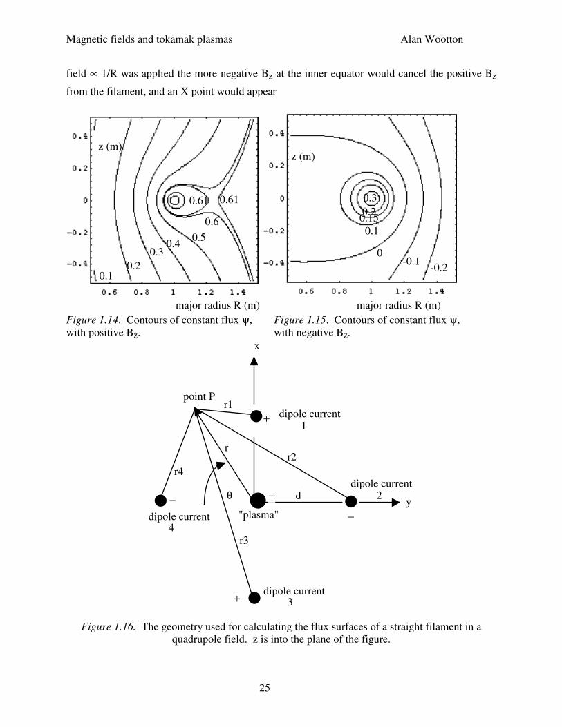
Magnetic fields and tokamak plasmas Alan Wootton
25
field ∝ 1/R was applied the more negative Bz at the inner equator would cancel the positive Bz
from the filament, and an X point would appear
z (m)
major radius R (m)
0.10.2
0.30.4
0.5
0.6
0.610.61
z (m)
major radius R (m)
-0.2-0.1
0
0.1
0.15
0.3
0.2
Figure 1.14. Contours of constant flux ψ, Figure 1.15. Contours of constant flux ψ,
with positive Bz. with negative Bz.
•
••
•
•+
+
−
−
+
x
y
r
θ
"plasma"
dipole currentdipole current
dipole current
dipole current
dipole current
1
2
3
4
point Pr1
r2
r3
r4
d
Figure 1.16. The geometry used for calculating the flux surfaces of a straight filament in a
quadrupole field. z is into the plane of the figure.
Magnetic fields and tokamak plasmas Alan Wootton
26
For a second example, consider the field lines and flux surfaces resulting from a quadrupole field
applied to a single filamentary current, in straight geometry. In a straight system the field lines
will lie in a surface defined by constant vector potential A (i.e. ψ constant, with R ⇒ ∞). The
single (“plasma”) filament of current Izp lies at the origin of a rectalinear coordinate system
(x,y,z) shown in Figure 1.16, where z will approximate the toroidal direction in a toroidal
system. The vector potential at P is given by Equation 1.55 as Azp = −µ 0I zp
2πln r( ), with r the
radius from the plasma filament to a point P. There are then four additional filaments, at a
distance d from the plasma filament, with currents Izq alternatingly + (into the plane) and - (out
of the plane). The ith additional filament (i = 1 to 4) has a vector potential Azqi = −µ 0I zq
2πln ri( ) in
its own local coordinate system. Transforming to the coordinate system (r,θ) we obtain
Az =−µ0 Izp
2πln r( ) +
µ 0Izq
2π
ln d 2 + r 2 − 2dr cos θ( )( )1 /2
+ ln d2 + r 2 + 2drcos θ( )( )1/ 2
− ln d2 + r 2 − 2drsin θ( )( )1/2
− ln d2 + r 2 + 2drsin θ( )( )1/2
1.57
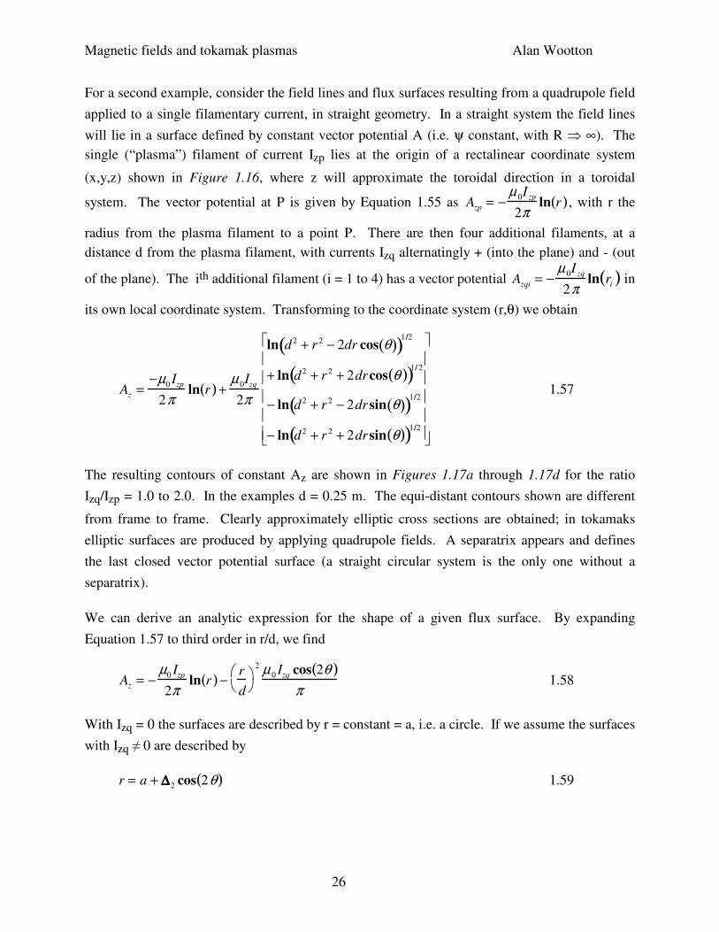
The resulting contours of constant Az are shown in Figures 1.17a through 1.17d for the ratio
Izq/Izp = 1.0 to 2.0. In the examples d = 0.25 m. The equi-distant contours shown are different
from frame to frame. Clearly approximately elliptic cross sections are obtained; in tokamaks
elliptic surfaces are produced by applying quadrupole fields. A separatrix appears and defines
the last closed vector potential surface (a straight circular system is the only one without a
separatrix).
We can derive an analytic expression for the shape of a given flux surface. By expanding
Equation 1.57 to third order in r/d, we find
Az = −µ0 Izp
2πln r( ) −
r
d
2 µ 0 Izq cos 2θ( )π
1.58
With Izq = 0 the surfaces are described by r = constant = a, i.e. a circle. If we assume the surfaces
with Izq ≠ 0 are described by
r = a + ∆∆∆∆2 cos 2θ( ) 1.59
Magnetic fields and tokamak plasmas Alan Wootton
27
Figure 1.17a. Vector potential contours with Figure 1.17a. Vector potential contours with
Izq/Izp = 1. The quadrupole filaments are at Izq/Izp = 2. The quadrupole filaments are at
± 0.25 m. ± 0.25 m.
then Equation 1.58 gives, after expanding in ∆/a,
−Az =µ0 Izp
2πln a( ) +
∆∆∆∆a
µ0 Izp
2πcos 2θ( )+
a
d
2 µ0I zq cos 2θ( )π
+a
d
2 ∆∆∆∆a
2µ 0 Izq cos2
2θ( )π
1.60
For a/d << 1, ∆/a << 1 we can ignore the last term (∝ cos2(2θ)). Then we ensure that
Az = const = −µ0I zp
2πln a( ) by setting the coefficient in front of the cos(2θ) to zero, i.e.
∆∆∆∆a
= 2I zq
I zp
a
d
2
1.61
The elongation of the surface is then
height
width=
1 + 2Izq
Izp
a
d
2
1 − 2Izq
Izp
a
d
2≈1 + 4
Izq
Izp
a
d
2
1.62
Magnetic fields and tokamak plasmas Alan Wootton
28
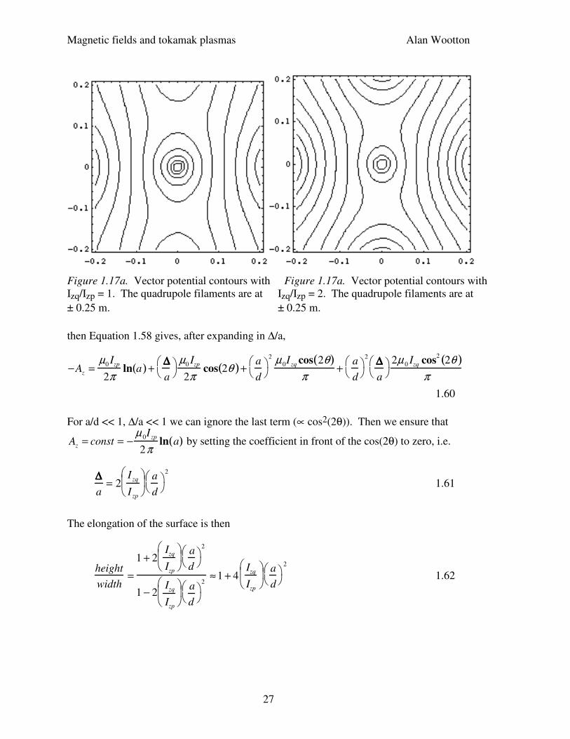
Figure 1.18a and 18b show the computed distortion to a particular surface (A = constant) for d
= 0.25, Izq/Izp = 0 and 2.0. With Izq/Izp = 1.0 the value of height to width is measured to be 1.28,
as compared to the value of 1.25 derived from Equation 1.62.
Figure 1.18a. Contours of vector potential Figure 1.18b Contours of vector potential
with Izq/Izp = 0. The larger contour is taken with Izq/Izp = 2. The contours have the same
as a reference in determining the distortion flux values as those shown in Figure 1.18a.
produced by an applied quadrupole field.
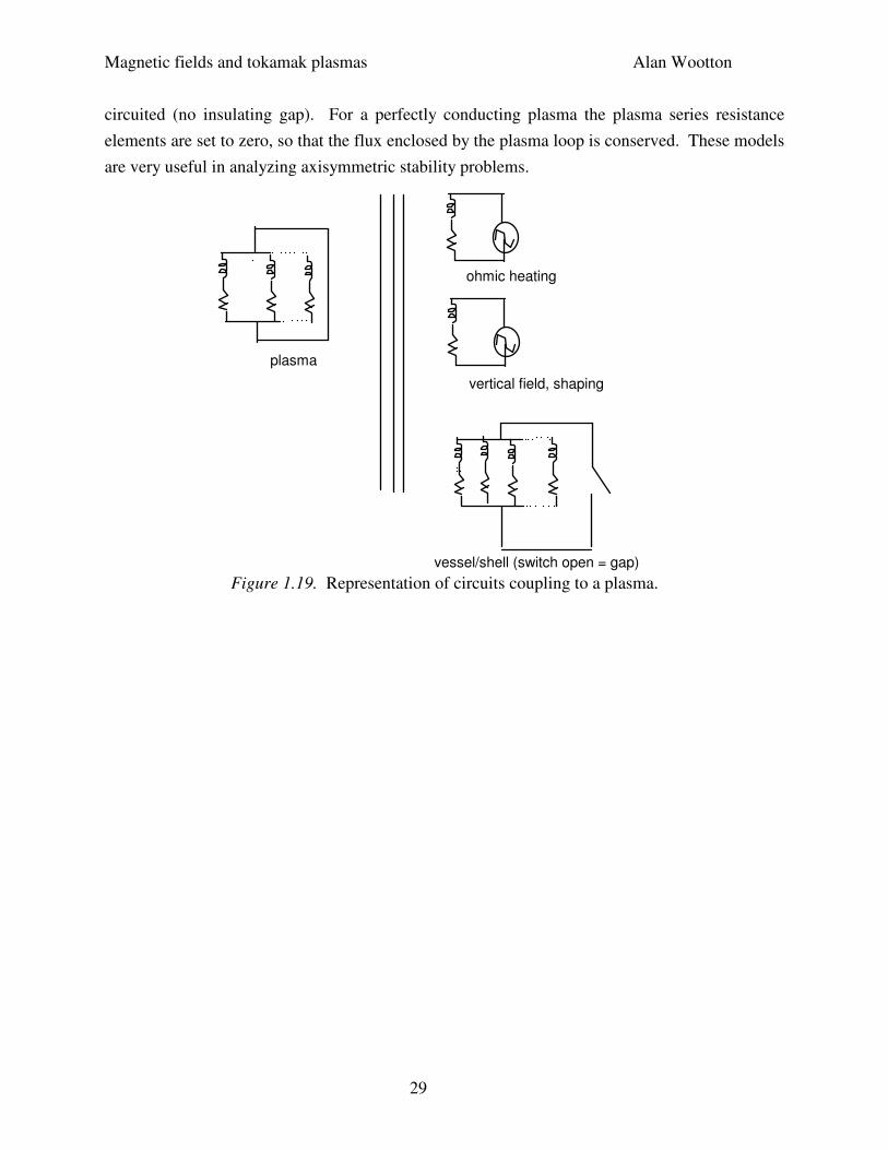
Circuit equations
For some applications we will consider the plasma as a lumped series resistance and inductance,
coupled to other circuits (including a conducting vacuum vessel) by mutual inductances. Figure
1.19 shows how this is represented.
The equation for circuit l consisting of a series self inductance Lll and resistance Ωl, coupled by
mutual inductances Mli to other circuits i, is
1.63
The sum over the mutual inductances is for i ≠ l because Mll = Lll is brought out separately. If
the circuit is closed (short circuited), then εl = 0. If the circuit is open, or connected to a high
input impedance, then Il = 0 and εl = d/dt(ΣMl,iIi). The plasma is sometimes represented as one
series inductance-resistance circuit, or sometimes as a number of such circuits in parallel, all
short circuited together. The vacuum vessel is similarly represented as a number of paralleled
resistor-inductor circuits, which can be open circuit (a vessel with an insulating gap) or short
Magnetic fields and tokamak plasmas Alan Wootton
29
circuited (no insulating gap). For a perfectly conducting plasma the plasma series resistance
elements are set to zero, so that the flux enclosed by the plasma loop is conserved. These models
are very useful in analyzing axisymmetric stability problems.
plasma
vessel/shell (switch open = gap)
ohmic heating
vertical field, shaping
Figure 1.19. Representation of circuits coupling to a plasma.
Magnetic fields and tokamak plasmas Alan Wootton
30
2. SOME NON STANDARD MEASUREMENT TECHNIQUES
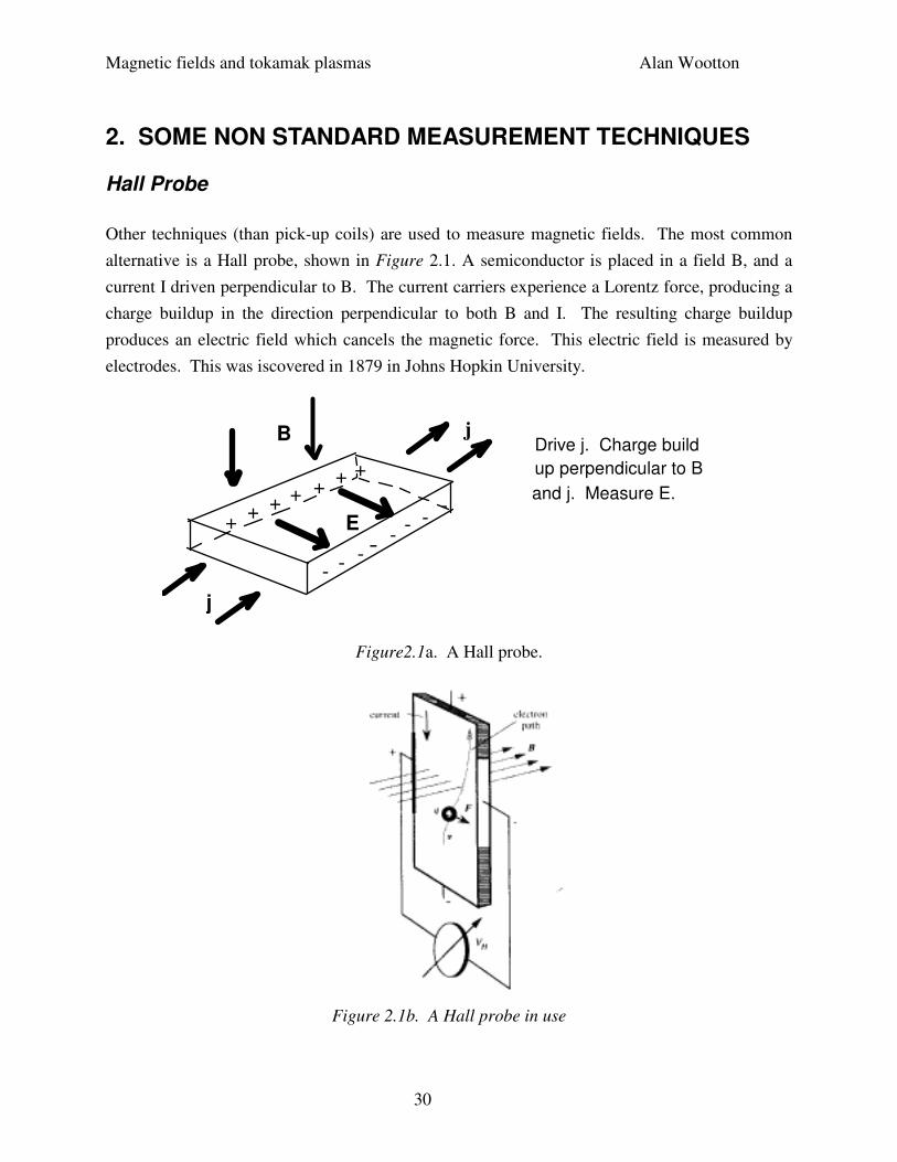
Hall Probe
Other techniques (than pick-up coils) are used to measure magnetic fields. The most common
alternative is a Hall probe, shown in Figure 2.1. A semiconductor is placed in a field B, and a
current I driven perpendicular to B. The current carriers experience a Lorentz force, producing a
charge buildup in the direction perpendicular to both B and I. The resulting charge buildup
produces an electric field which cancels the magnetic force. This electric field is measured by
electrodes. This was iscovered in 1879 in Johns Hopkin University.
B
j
E++ + + +
+ +
- - --
- --
Drive j. Charge build
up perpendicular to B
and j. Measure E.
-
j
Figure2.1a. A Hall probe.
Figure 2.1b. A Hall probe in use
Magnetic fields and tokamak plasmas Alan Wootton
31
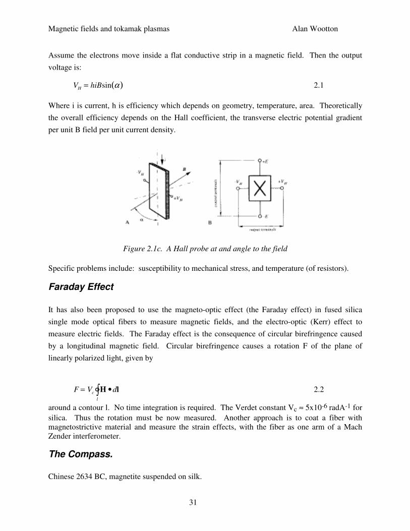
Assume the electrons move inside a flat conductive strip in a magnetic field. Then the output
voltage is:
VH = hiBsin α( ) 2.1
Where i is current, h is efficiency which depends on geometry, temperature, area. Theoretically
the overall efficiency depends on the Hall coefficient, the transverse electric potential gradient
per unit B field per unit current density.
Figure 2.1c. A Hall probe at and angle to the field
Specific problems include: susceptibility to mechanical stress, and temperature (of resistors).
Faraday Effect
It has also been proposed to use the magneto-optic effect (the Faraday effect) in fused silica
single mode optical fibers to measure magnetic fields, and the electro-optic (Kerr) effect to
measure electric fields. The Faraday effect is the consequence of circular birefringence caused
by a longitudinal magnetic field. Circular birefringence causes a rotation F of the plane of
linearly polarized light, given by
F = Vc H •dll
∫ 2.2
around a contour l. No time integration is required. The Verdet constant Vc ≈ 5x10⁻⁶ radA-1 for
silica. Thus the rotation must be now measured. Another approach is to coat a fiber with
magnetostrictive material and measure the strain effects, with the fiber as one arm of a Mach
Zender interferometer.
The Compass.
Chinese 2634 BC, magnetite suspended on silk.
Magnetic fields and tokamak plasmas Alan Wootton
32
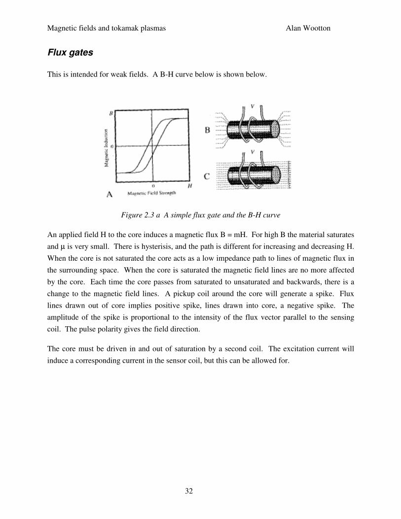
Flux gates
This is intended for weak fields. A B-H curve below is shown below.
Figure 2.3 a A simple flux gate and the B-H curve
An applied field H to the core induces a magnetic flux B = mH. For high B the material saturates
and µ is very small. There is hysterisis, and the path is different for increasing and decreasing H.
When the core is not saturated the core acts as a low impedance path to lines of magnetic flux in
the surrounding space. When the core is saturated the magnetic field lines are no more affected
by the core. Each time the core passes from saturated to unsaturated and backwards, there is a
change to the magnetic field lines. A pickup coil around the core will generate a spike. Flux
lines drawn out of core implies positive spike, lines drawn into core, a negative spike. The
amplitude of the spike is proportional to the intensity of the flux vector parallel to the sensing
coil. The pulse polarity gives the field direction.
The core must be driven in and out of saturation by a second coil. The excitation current will
induce a corresponding current in the sensor coil, but this can be allowed for.
Magnetic fields and tokamak plasmas Alan Wootton
33
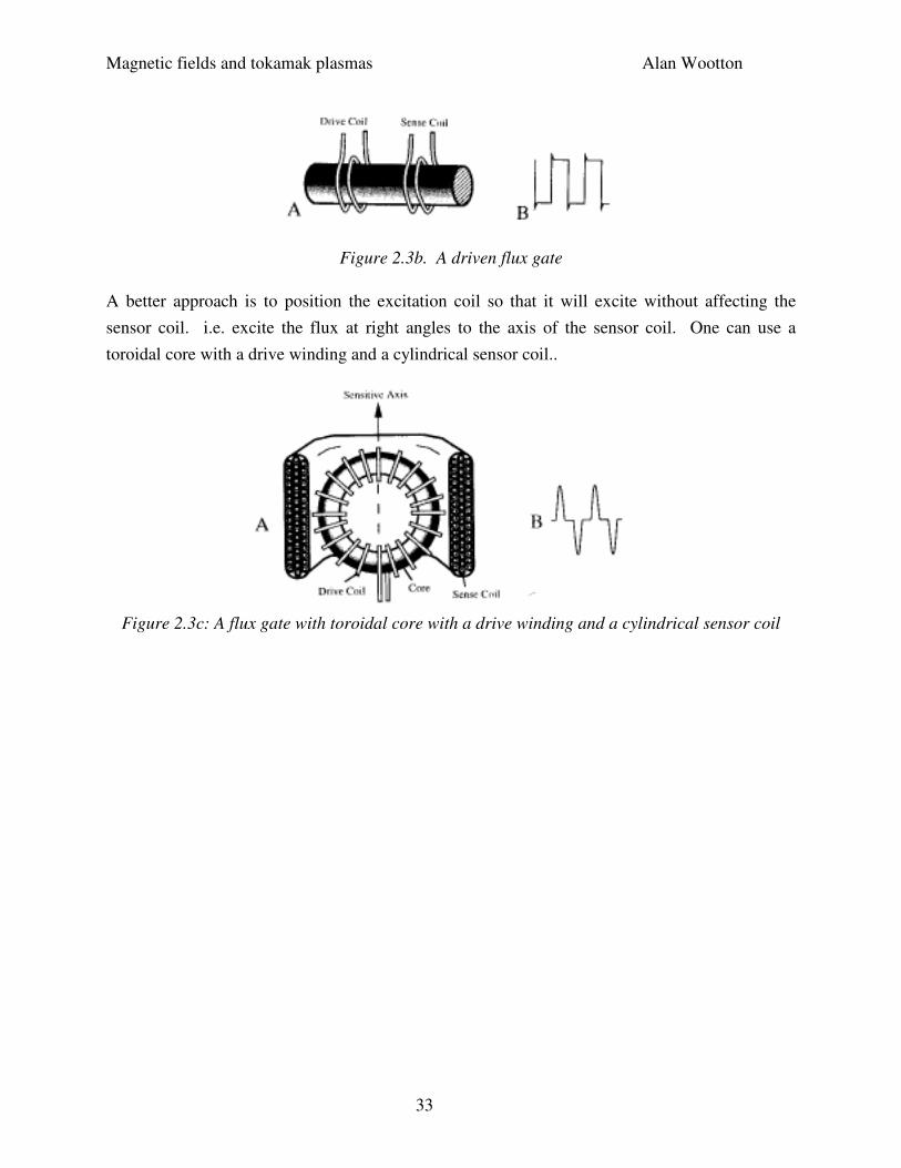
Figure 2.3b. A driven flux gate
A better approach is to position the excitation coil so that it will excite without affecting the
sensor coil. i.e. excite the flux at right angles to the axis of the sensor coil. One can use a
toroidal core with a drive winding and a cylindrical sensor coil..
Figure 2.3c: A flux gate with toroidal core with a drive winding and a cylindrical sensor coil
Magnetic fields and tokamak plasmas Alan Wootton
34
3. GENERAL FIELD CHARACTERIZATION
Fourier components
Suppose we want to characterize the tangential (subscript τ) and normal (subscript n) fields on a
circular contour of radius al. It is often convenient to express the results as a Fourier series: for
the poloidal (θ) and radial (ρ) fields outside a current I we can write
Bω = Bτ =µ0I
2πal
1 + λ n cos nω( ) + δn sin(nω )n
∑
3.1
Bρ = Bn =µ 0 I
2πal
κn cos nω( ) + µ n sin(nω )n
∑
3.2
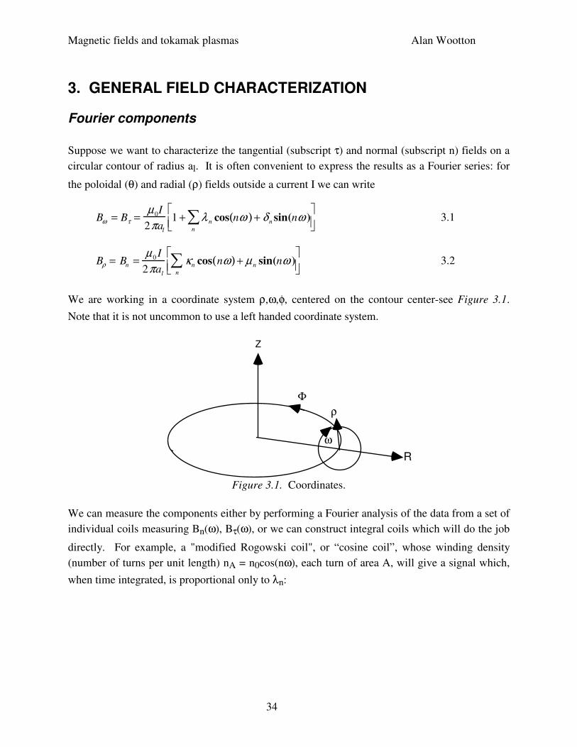
We are working in a coordinate system ρ,ω,φ, centered on the contour center-see Figure 3.1.
Note that it is not uncommon to use a left handed coordinate system.
Φ
R
Z
ρ
ω
Figure 3.1. Coordinates.
We can measure the components either by performing a Fourier analysis of the data from a set of
individual coils measuring Bn(ω), Bτ(ω), or we can construct integral coils which will do the job
directly. For example, a "modified Rogowski coil", or “cosine coil”, whose winding density
(number of turns per unit length) nA = n0cos(nω), each turn of area A, will give a signal which,
when time integrated, is proportional only to λn:
Magnetic fields and tokamak plasmas Alan Wootton
35
ε = −d
dtB •nSdS( )
S
∫ = −d
dtBω (ω )nA (ω )al Adω( )
0
2π
∫
= −µ0 An0
2πd
dtI cos(nω ) 1 + λ n sin(nω ) + µ n cos(nω )
n
∑
0
2π
∫ dω
= − µ0 An0
2
d
dtIλn
3.3
The elemental area dS = nAAdl, the unit length dl = aldω, and ns is the unit normal to the coil
area. That is, the only contribution to the space integral comes from the term cos2(nω), because
∫0
2πcos(nω)cos(mω)dω = π if m = n, otherwise = 0. If the winding density is proportional to
sin(nω), the time integrated output is proportional to δn. To obtain the coefficients µn and κn, we
must wind a “saddle coil” with nw turns of width w varying as sin(nω) or cos(nω), so that for a
”sin” saddle coil w(ω) = w0 cos(ω), and
ε = − d
dtB(ω )nw w(ω )aldω( )∫
= −µ
0w0nw
2
d
dtIµ n
3.4
In this case the elemental area dS = nwwdl = nwwaldω, the time integrated output provides the
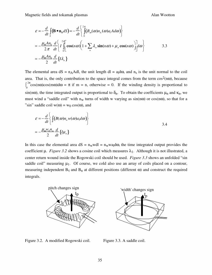
coefficient µ. Figure 3.2 shows a cosine coil which measures λ1. Although it is not illustrated, a
center return wound inside the Rogowski coil should be used. Figure 3.3 shows an unfolded “sin
saddle coil” measuring µ1. Of course, we cold also use an array of coils placed on a contour,
measuring independent Bτ and Bn at different positions (different ω) and construct the required
integrals.
pitch changes sign 'width' changes signp pI
I
Figure 3.2. A modified Rogowski coil. Figure 3.3. A saddle coil.
Magnetic fields and tokamak plasmas Alan Wootton
36
Field components on a rectangle
If we want to characterize the fields on a rectangular contour, we can make use of the fact that an
arbitrary function in a plane can be expressed as
B(η,ξ ) = cm, pξmη p
m, p
∑ 3.5
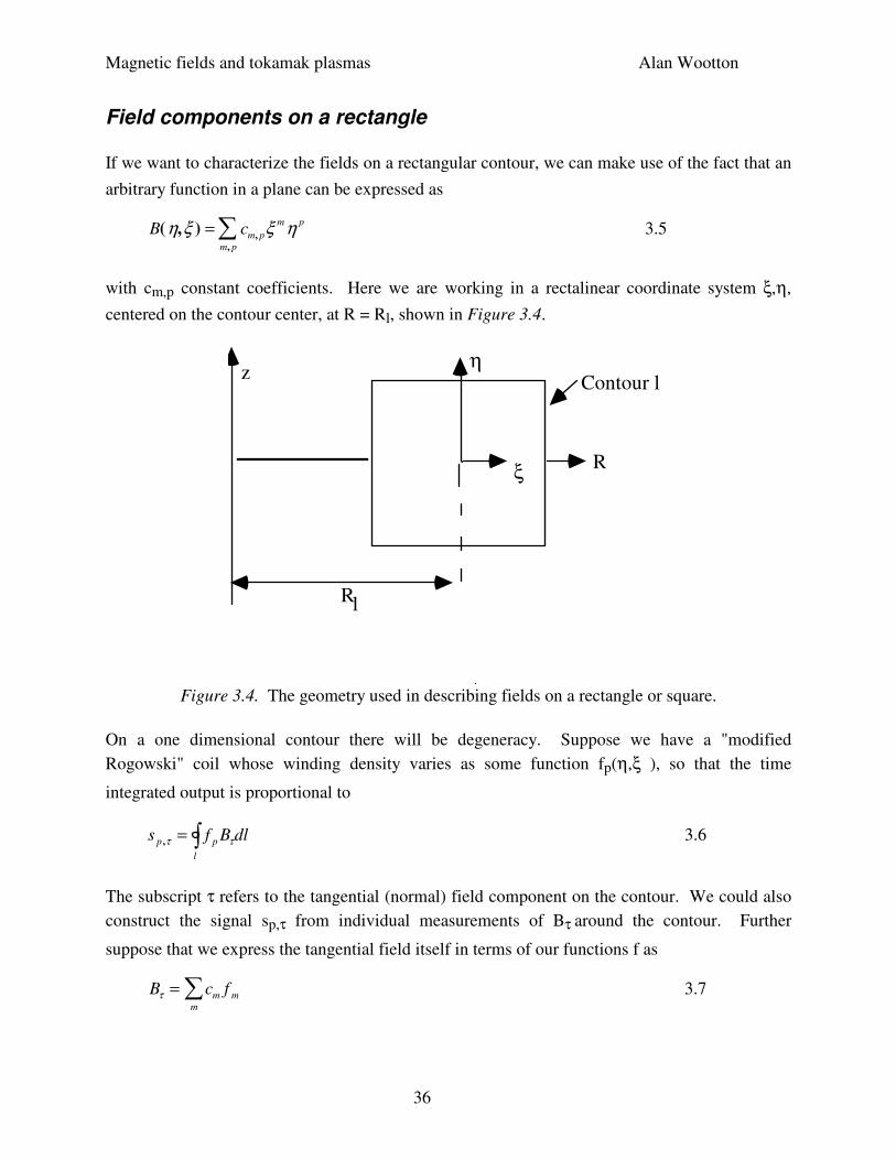
with cm,p constant coefficients. Here we are working in a rectalinear coordinate system ξ,η,
centered on the contour center, at R = Rl, shown in Figure 3.4.
η
ξ
Rl
z
R
Contour l
Figure 3.4. The geometry used in describing fields on a rectangle or square.
On a one dimensional contour there will be degeneracy. Suppose we have a "modified
Rogowski" coil whose winding density varies as some function fp(η,ξ ), so that the time
integrated output is proportional to
s p ,τ = f p Bτdll
∫ 3.6
The subscript τ refers to the tangential (normal) field component on the contour. We could also
construct the signal sp,τ from individual measurements of Bτ around the contour. Further
suppose that we express the tangential field itself in terms of our functions f as
Bτ = cm f m
m
∑ 3.7
Magnetic fields and tokamak plasmas Alan Wootton
37
Then we can write
s p ,τ = cm
m
∑ fm f p dll
∫ 3.8
i.e. if we can calculate ∫lfmfpdl for our chosen functions f, then we can express the coefficients cm
through the measured parameters sp,τ. In a similar way we can build a saddle coil of width fp
whose time integrated output is then
s p ,n = f pBndll
∫ 3.9
Expressing the normal field as
Bn = dm f m
m
∑ 3.10
we have
s p ,n = dm
m
∑ f m f pdll
∫ 3.11
Again, assuming we can calculate ∫lfmfpdl, the coefficients dm can be expressed in terms of the
measured sp,n.
We still have to choose the functions fp. One choice, which is used in 'multipole moments',
discussed later, is ρp, the pth power of a vector radius on the contour l. This can be expressed in
the form of a complex number as
ρ = ξ + iη 3.12
e.g. for p = 2 we have
ρ2 = ξ2 − η2 + i ξη( ) 3.13
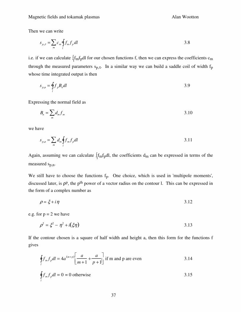
If the contour chosen is a square of half width and height a, then this form for the functions f
gives
f m
l
∫ f pdl = 4am + p( ) a
m +1+
a
p +1
if m and p are even 3.14
f m
l
∫ f pdl = 0 = 0 otherwise 3.15
Magnetic fields and tokamak plasmas Alan Wootton
38
Then we would have the output from the 'modified Rogowski' coil
s p ,τ = cm fm
l
∫ f p dm
∑ l
= cm 4am + p( ) a
m + 1+ a
p +1
m
∑ for m, p even 3.16
= 0 otherwise 3.17
Equations 3.16 and 3.17 show specifically how, by including a finite number of terms (say pmax
= mmax = 5) we will end up with a set of linear equations relating the measured signals to the
required constants cm. We must now solve them to obtain the coefficients cm as functions of the
measured sp,τ; a similar procedure provides the dm as functions of the signals sp,n. The result is
not as elegant as the Fourier analysis applicable on a circular contour, where a single coil can be
wound to measure each individual Fourier coefficient, but I don’t know another way to represent
the fields on a square contour. Of course, instead of using these specially wound coils to
measure sp,τ and sp,n directly, the required integrals can always be constructed from individual
coil signals of Bτ and Bn around the contour l.
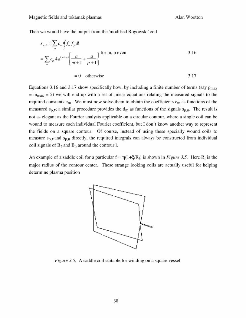
An example of a saddle coil for a particular f = η(1+ξ/Rl) is shown in Figure 3.5. Here Rl is the
major radius of the contour center. These strange looking coils are actually useful for helping
determine plasma position
Figure 3.5. A saddle coil suitable for winding on a square vessel
Magnetic fields and tokamak plasmas Alan Wootton
39
4. PLASMA CURRENT
Rogowski coil
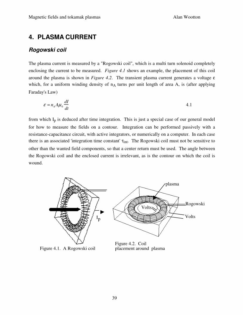
The plasma current is measured by a "Rogowski coil", which is a multi turn solenoid completely
enclosing the current to be measured. Figure 4.1 shows an example, the placement of this coil
around the plasma is shown in Figure 4.2. The transient plasma current generates a voltage ε
which, for a uniform winding density of nA turns per unit length of area A, is (after applying
Faraday's Law)
ε = nA Aµ0
dI
dt 4.1
from which Ip is deduced after time integration. This is just a special case of our general model
for how to measure the fields on a contour. Integration can be performed passively with a
resistance-capacitance circuit, with active integrators, or numerically on a computer. In each case
there is an associated 'integration time constant' τint. The Rogowski coil must not be sensitive to
other than the wanted field components, so that a center return must be used. The angle between
the Rogowski coil and the enclosed current is irrelevant, as is the contour on which the coil is
wound.
Figure 4.1. A Rogowski coil
Ip
Rogowski
Volts
Volts
Figure 4.2. Coil placement around plasma
plasma
Magnetic fields and tokamak plasmas Alan Wootton
40
5. LOOP VOLTS, VOLTS per TURN, SURFACE VOLTAGE.
Introduction
The Loop Volts εl, also called the Volts per Turn or Surface Voltage, is used in calculating the
Ohmic power input to the plasma. It also allows a calculation of the plasma resistivity Ωp. εl is
also a useful measure of cleanliness: clean ohmic heated tokamaks usually have εl ~ 1.5V.
What we want to measure is the resistive voltage drop across or around a plasma. In a linear
machine, this simply done by measuring the potential across the end electrodes with a resistive
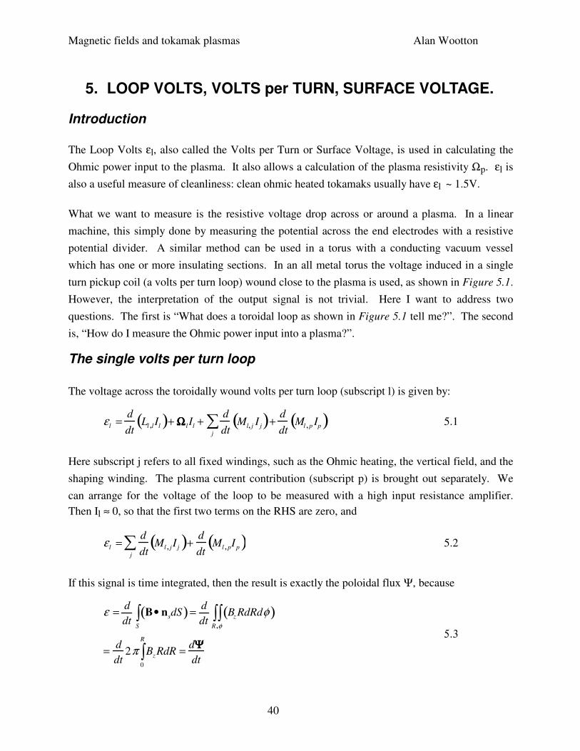
potential divider. A similar method can be used in a torus with a conducting vacuum vessel
which has one or more insulating sections. In an all metal torus the voltage induced in a single
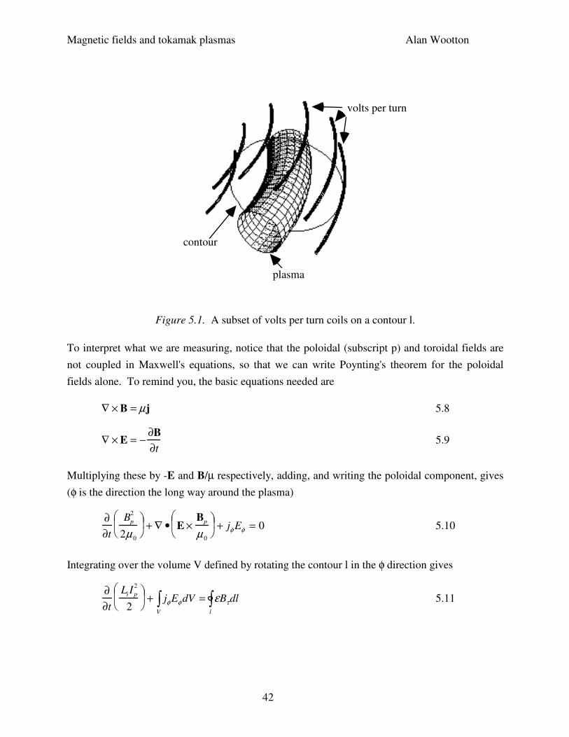
turn pickup coil (a volts per turn loop) wound close to the plasma is used, as shown in Figure 5.1.
However, the interpretation of the output signal is not trivial. Here I want to address two
questions. The first is “What does a toroidal loop as shown in Figure 5.1 tell me?”. The second
is, “How do I measure the Ohmic power input into a plasma?”.
The single volts per turn loop
The voltage across the toroidally wound volts per turn loop (subscript l) is given by:
ε l =d
dtLl ,lIl( )+ ΩΩΩΩ lIl +
d
dtMl, j I j( )
j
∑ +d
dtMl , p Ip( ) 5.1
Here subscript j refers to all fixed windings, such as the Ohmic heating, the vertical field, and the
shaping winding. The plasma current contribution (subscript p) is brought out separately. We
can arrange for the voltage of the loop to be measured with a high input resistance amplifier.
Then Il ≈ 0, so that the first two terms on the RHS are zero, and
ε l =d
dtMl , jI j( )
j
∑ +d
dtMl , pIp( ) 5.2
If this signal is time integrated, then the result is exactly the poloidal flux Ψ, because
ε = d
dtB• nsdS( )
S
∫ = d
dtBz RdRdφ( )
R ,φ∫∫
= d
dt2π Bz RdR
0
R
∫ = dΨΨΨΨdt
5.3
Magnetic fields and tokamak plasmas Alan Wootton
41
Now consider the voltage εp around the plasma. It is connected on itself (a torus) so that:
ε p = 0 =d
dtLp, pIp( )+ ΩΩΩΩ pIp +
d
dtM p, jI j( )
j
∑ 5.4
Now remembering the definition of mutual inductance in terms of linked fluxes, we can always
write the flux through circuit i due to current Ij in circuit j as the flux through another circuit k
due to the current Ij in circuit j plus the incremental flux between the circuits k and i due to the
current Ij in circuit j, ∆Ψk,i;j. Then
Mi, j I j = Mk , jI j + ∆Ψ∆Ψ∆Ψ∆Ψ k ,i; j = M j ,k I j + ∆Ψ∆Ψ∆Ψ∆Ψ k ,i; j 5.5
Then for example Ml,ohIoh = Mp,ohIoh + ∆Ψp,l;oh
Thus we can write
ε l =d
dtM p, jI j( )
j
∑ +d
dtMl , pI p( )+
d
dt∆Ψ∆Ψ∆Ψ∆Ψp,l ; j( )
j
∑ 5.6
Substituting from Equation 5.4 gives
ε l = −d
dtLp, p Ip( )− ΩΩΩΩpIp +
d
dtΨΨΨΨ plasma−loop( ) 5.7
where ∆Ψplasma-loop is now the total flux between the loop and the plasma, provided by all
circuits, including the plasma (plasma, ohmic heating, vertical field, shaping). If the plasma
current is constant the volts per turn loop tells us the plasma resistance. A more elegant approach
to seeing this is to use Poynting’s theorem.
Poynting’s theorem
Consider a number of non integrated flux loops, i.e. volts per turn loops, measuring dΨ/dt, all
placed around the plasma on some contour l, which might be the vacuum vessel. Figure 5.1
shows the configuration. Note that the emf ε = -2πREφ will not necessarily be the same in each
loop, because the contour l is not necessarily on a magnetic surface.
Magnetic fields and tokamak plasmas Alan Wootton
42
plasma
volts per turn
contour
Figure 5.1. A subset of volts per turn coils on a contour l.
To interpret what we are measuring, notice that the poloidal (subscript p) and toroidal fields are
not coupled in Maxwell's equations, so that we can write Poynting's theorem for the poloidal
fields alone. To remind you, the basic equations needed are
∇ × B = µj 5.8
∇ × E = −∂B
∂t 5.9
Multiplying these by -E and B/µ respectively, adding, and writing the poloidal component, gives
(φ is the direction the long way around the plasma)
∂∂t
Bp
2
2µ 0
+ ∇ • E ×
Bp
µ 0
+ jφ Eφ = 0 5.10
Integrating over the volume V defined by rotating the contour l in the φ direction gives
∂∂t
LiI p
2
2
+ jφ Eφ dV = εBτdl
l
∫V
∫ 5.11
Magnetic fields and tokamak plasmas Alan Wootton
43
Here we have used ∇ • E × Bp( )dV =V
∫ Eφ × Bp( )• dSφ =S
∫ 2πREφ BpdlS
∫ . Li is defined by (LiIp2)/2
= ∫(Bp2/(2µ0)dV. Note the integration is to the contour l, not the plasma edge. Therefore the
inductance is not just that internal to the plasma, which is usually called li. Now use Ohms law
j.B = σ||E.B, and assuming |Bφ0-Bφ| << Bφ0 gives Eφ = jφ/σ||. Therefore
∂∂t
LiI p
2
2
+
jφ2
σ ||
dV = Ip
V
∫ ε 5.12
where
ε =1
µ0Ip
εBτ dll
∫ 5.13
What we find, from Equation 5.12, is that the ohmic input power ∫jφ2/σ||dV into the plasma must
be evaluated knowing the poloidal distribution of both ε and Bτ around the contour l, as well as
the inductance Li within that contour. For example, suppose the contour is a circle of radius al,
and
ε = ε0 1 + ε n cos nω( )n
∑
5.14
Bτ =µ 0 Ip
2πal
1+ λn cos nω( )n
∑
5.15
Then we obtain
ε = ε0 1+ λnε n
n
∑
5.16
The inductance Li is given approximately by (i.e. the "straight" circular tokamak )
Li ≈ µ0 Rp lnal
ap
+
li
2
5.17
with ap, Rp the plasma minor, major radius. The term µ0/(4π)li is the inductance per unit length
(toroidally) inside the plasma, and the ln term represents the inductance between the plasma
surface (r = ap) and the contour l (r = al). The approximation given is for a straight circular
tokamak coaxial with a circular contour. That part of the inductance between the plasma and the
contour is sensitive to plasma position.
Magnetic fields and tokamak plasmas Alan Wootton
44
Uses of the Volts per turn measurement
We can deduce an average value of the plasma conductivity, <σ>, by writing
2πRpI p
2
πap
2 σ=
jφ2
σ ||V
∫ dV = Ip ε −∂∂t
LiIp
2
2
5.18
From this we can define a conductivity temperature Tσ. The conductivity deduced by Spitzer for
Coulomb collisions is given by (there are corrections for the fact that, in a torus, trapped particles
cannot carry current and so σ must be reduced)
σ = 1.9 ×10⁴ Te
32
Zeff ln ΛΛΛΛs( ) 5.19
Then Tσ is defined as that temperature which gives a Spitzer conductivity (with Zeff = 1) equal to
the average conductivity <σ>, with an approximate value taken for ln(Λs). We can also derive an
average “skin time”, from the formula for the penetration of a field into a conductor of uniform
conductivity <σ>:
τskin =πµ0σa p
2
16 5.20
The definition of energy confinement time for an ohmic heated plasma with major radius Rp,
cross sectional area Sφ.(here we assume a circular minor radius ap, so Sφ = πap2), total energy
content W = 3πRp∫SφpdSφ, ohmic input power Poh = Ip2Ωp, can we written in terms of the
poloidal beta value βI = 8π/(µ0Ip2)∫Sφ
pdSφ (discussed later) as
τ E =W
Poh
=3µ0βI Rp
8ΩΩΩΩ p
=3µ 0βI ap
2 σ16
τ 5.21
Combining equations 5.20 and 5.21 shows that
τE
τskin
≈ βI 5.22
Therefore for ohmic heated plasmas, where typically βI ≈ 0.3, the currents penetrate
approximately 3 times slower than the energy escapes from the plasma.
Magnetic fields and tokamak plasmas Alan Wootton
45
6. TOKAMAK EQUILIBRIA
6.0. AN INTUITIVE DERIVATION OF TOKAMAK EQUILIBRIUM
Introduction
After having described how to measure the plasma current and loop voltage, the next most
important parameter to measure is the plasma position. We will show how we determine both
this, and certain integrals of the pressure and field across the plasma cross section (specifically βI
+ li/2), in section 7. The basic idea is that we want an expression for the fields outside the plasma
in terms of plasma displacement ∆ and (βI + li/2). We can only do this by knowing a solution to
the plasma equilibrium, i.e. we must solve the Grad Shafranov equation. I deal with this later in
this section, but first we can gain a physical picture of tokamak equilibrium by considering the
various forces acting on a toroidal plasma. Also note that there are techniques to measure plasma
position without recourse to equilibrium solutions, the so called “moments” method. However,
the interpretation of this method (i.e. what has been measured) itself requires a knowledge of the
equilibrium.
The total energy of our system must be made up of 3 parts,
W = Wp + W1
B + W 2
B 6.0.1
where WP is the energy stored as pressure, W1B is the energy stored in toroidal fields (poloidal
currents), and W2B is the energy stored in poloidal fields (toroidal currents). Once we have
calculated expressions for these terms, we can obtain the required forces: the minor radial force
Fa = ∂W/∂a, and the major radial force FR = ∂W/∂R. By setting the net force = 0 we will obtain
the conditions necessary for equilibrium. We work with a circular cross sectioned plasma with
major radius R and a minor radius a, and a/R << 1. Figure 6.0.1 shows the geometry. The
poloidal coordinate is θ. We use <...> to mean an average over the volume (which is the same as
an average over the plasma surface if a/R << 1) and V = 2πRπa2. A positive force is in the “R”
or “a” direction (an expansion).
Magnetic fields and tokamak plasmas Alan Wootton
46
pp
BφiBφi
Bφe
dφ
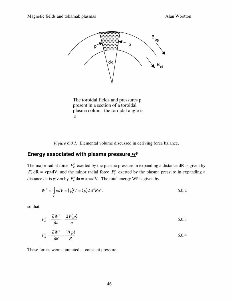
The toroidal fields and pressures p present in a section of a toroidal plasma colum. the toroidal angle is
φ
Figure 6.0.1. Elemental volume discussed in deriving force balance.
Energy associated with plasma pressure WP
The major radial force FR
p exerted by the plasma pressure in expanding a distance dR is given by
FR
pdR = <p>dV, and the minor radial force Fa
p exerted by the plasma pressure in expanding a
distance da is given by Fa
pda = <p>dV. The total energy Wp is given by
Wp = pdV
V
∫ = p V = p 2π 2Ra
2: 6.0.2
so that
Fa
p =∂W p
∂a=
2V p
a 6.0.3
FR
p =∂W p
∂R=
V p
R 6.0.4
These forces were computed at constant pressure.
Magnetic fields and tokamak plasmas Alan Wootton
47
Energy associated with toroidal fields W1B
The energy associated with poloidal currents is written as
W1
B =L1I1
2
2+
L1eI1e
2
2+ M1I1I1e 6.0.5
Here I1 is the poloidal current in the plasma, and I1e is the poloidal current in the toroidal field
coil (subscript e for external). I1 is that poloidal current flowing in the plasma edge which
produces a toroidal field equal to the difference between the internal toroidal field Bφi and the
external toroidal field Bφe. By definition we have
L1I1
2
2=
Bφi − Bφe( )2
V
2µ 0
6.0.6
M1I1I1e =Bφi − Bφe( )BφeV
µ0
6.0.7
Now the circuits I1 and I1e are perfectly coupled, so that L1 = M1. The field B1 = µ0I1/(2πR), and
so
M1 = L1 =1
I1
2
B1
2
µ 0
dVV
∫ = µ0 R − R2 − a
2( )12
≈
µ 0a2
2R 6.0.8
for skin currents. To get the forces we will need only the functional dependencies, namely
∂L1
∂a=
2 L1
a
∂M1
∂a=
2M1
a
6.0.9
∂L1
∂R= −
L1
R
∂M1
∂R= −
M1
R
6.0.10
The forces will be computed at constant current. For example, the part of the force due to
∂/∂R(L1I12/2) is then written as (I12/2)∂/∂R(L1) = -(I12/2)L/R = -(L1I12/2)(1/R). Using Equation
6.0.6 this becomes (I12/2)∂/∂R(L1) = <Bφi-Bφe)2>V/(2Rµ0). Doing this for each component in
Equation 6.0.5 gives
Magnetic fields and tokamak plasmas Alan Wootton
48
F1a
B =∂W1
B
∂a=
2V
a
Bφi
2 − Bφe
2( )2µ 0
6.0.11
F1R
B =∂W1
B
∂R=
V
R
Bφe
2 − Bφi
2( )2µ0
6.0.12
There will be no force from the term L1eI1e2/2, because we keep the external currents constant.
Energy associated with poloidal fields W2B
Again we write the energy in the poloidal circuits as
W2
B =L2I2
2
2+
L2 eI2e
2
2+ M2 I2 I2e 6.0.13
with I2 = Ip the toroidal plasma current, and I2e the poloidal currents in external windings. These
windings are imagined to consist of a set which provides an external vertical field Bz but induces
no plasma current, and a set which drives the plasma current but produces no Bz. We will need
the radial derivatives (with respect to both major and minor radii) of the self and mutual
inductances. All external currents will be kept fixed, so that ∂(L2e)/∂a = ∂(L2e)/∂R = 0. Only
that winding producing a vertical field is imagined coupled through a mutual inductance to the
plasma.
We must make use of the inductance of a current loop:
L2
B = µ0R ln8R
a
− 2 +
li
2
6.0.14
The term li accounts for the inductance between the center of the loop and the edge, at r = a. We
also need the flux Ψ = M2I2e, the external flux passing through the central aperture, which can be
written as
ΨΨΨΨ = 2πRBz dR0
R
∫ 6.0.15
Then we have
∂L2
∂R= µ0 ln
8R
a
−1 +
l1
2
6.0.16
Magnetic fields and tokamak plasmas Alan Wootton
49
∂L2
∂a= −
µ0R
a 6.0.17
∂M2
∂R=
∂∂R
ΨΨΨΨI2e
=
2πRBz
I2e
6.0.18
∂M2
∂a=
∂∂a
ΨΨΨΨI2e
= 0 6.0.19
Now we can deduce the forces:
F2a
B =∂W 2
B
∂a= −
2V
a
Bθa
2
2µ 0
6.0.20
F2R
B =∂W2
B
∂R=
V
R
Bθa
2
µ 0
ln8R
a
−1+
li
2
+
2Bz Bθa R
µ0a
6.0.21
where
Bθa =µ 0 I2
2πa=
µ 0Ip
2πa 6.0.22
Total forces
We can now add Equations 6.0.3, 6.0.11 and 6.0.20 to get Fa, and Equations 6.0.4, 6.0.12 and
6.0.21 to get FR:
Fa =2V
a−
Bθa
2
2µ0
+Bφi
2 − Bφe
2( )2µ0
+ p
6.0.23
FR =V
R
Bθa
2
µ 0
ln8R
a
−1 +
li
2
+
2RBz Bθa
µ 0a+
Bφe
2 − Bφi
2( )2µ 0
+ p
6.0.24
with Bθa =µ0 Ip
2πa. Equilibrium requires Fa = 0, so that
p =Bθa
2
2µ0
+Bφe
2 − Bφi
2( )2µ0
+
6.0.25
Magnetic fields and tokamak plasmas Alan Wootton
50
Therefore if we can measure the difference in toroidal field with and without (when Bφi = Bφe)
plasma present, we can measure the average plasma pressure. This is discussed later in dealing
with “diamagnetism”.
The condition FR = 0 specifies the vertical field:
Bz = −aBθa
2Rln
8R
a
−
3
2+
li
2+
2µ0 p
Bθa
2
= −aBθa
2Rln
8R
a
−
3
2+
li
2+ βI
- 6.0.26
This was the field we used in section 1, Field lines and flux surfaces, to plot out the flux surfaces
which result from a combined circular filament and a vertical field.
6.1. THE FLUX OUTSIDE A CIRCULAR TOKAMAK
Later we will use the expression for the flux outside a circular tokamak. It can be considered to
come from two sources, that from the external maintaining fields ψext and that from the plasma
itself, ψp. In the previous section we derived an expression for the vertical field Bz necessary to
maintain a circular equilibrium (Equation 6.0.26). While the major radial term appearing as
ln8R
a
in Equation 6.0.26 clearly refers to the geometric center Rg (it comes from the
inductance of a plasma with radius a with a geometric center Rg), it is not obvious to what radius
the term outside the square brackets refers. It could be either Rg, or the coordinate itself, so that
Bz ∝ 1/R. In the former case, in a right-handed cylindrical coordinate system (R,φ,z), the flux
would be derived from ψ ∝ R2, or in our local coordinate system (ρ,ω,φ) based on Rg (See
Figure 1.7)
ψ = k0 + k1 cos ω( ) + k2 cos 2ω( ) 6.1.1
with ki a constant. The constant is unimportant, but the cos(2ω) term means that such an external
field would introduce ellipticity, and we have specifically considered a circular plasma.
Therefore we must take Bz ∝ 1/R, and in the coordinate system (R,φ,z) this is derived from a flux
ψ ext =µ 0I p R
4πln
8Rg
a
+ ΛΛΛΛ − 0.5
6.1.2
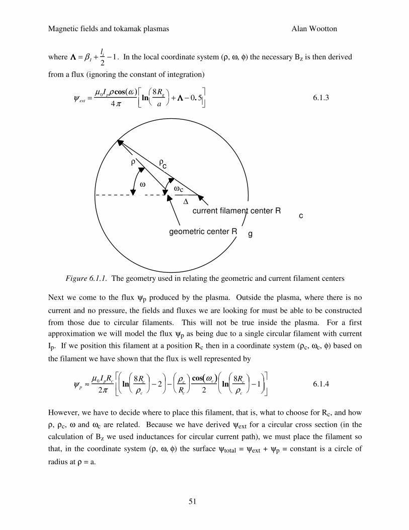
Magnetic fields and tokamak plasmas Alan Wootton
51
where ΛΛΛΛ = β I +li
2−1. In the local coordinate system (ρ, ω, φ) the necessary Bz is then derived
from a flux (ignoring the constant of integration)
ψ ext =µ 0I pρcos ω( )
4πln
8Rg
a
+ ΛΛΛΛ − 0. 5
6.1.3
∆
ρc
ρ
ω ω
current filament center Rc
geometric center R g
c
Figure 6.1.1. The geometry used in relating the geometric and current filament centers
Next we come to the flux ψp produced by the plasma. Outside the plasma, where there is no
current and no pressure, the fields and fluxes we are looking for must be able to be constructed
from those due to circular filaments. This will not be true inside the plasma. For a first
approximation we will model the flux ψp as being due to a single circular filament with current
Ip. If we position this filament at a position Rc then in a coordinate system (ρc, ωc, φ) based on
the filament we have shown that the flux is well represented by
ψ p ≈µ0 I pRc
2πln
8Rc
ρc
− 2
−
ρc
Rc
cos ωc( )
2ln
8Rc
ρc
−1
6.1.4
However, we have to decide where to place this filament, that is, what to choose for Rc, and how
ρ, ρc, ω and ωc are related. Because we have derived ψext for a circular cross section (in the
calculation of Bz we used inductances for circular current path), we must place the filament so
that, in the coordinate system (ρ, ω, φ) the surface ψtotal = ψext + ψp = constant is a circle of
radius at ρ = a.
Magnetic fields and tokamak plasmas Alan Wootton
52
Suppose we place the filament at a position R0 = Rc + ∆. From Figure 6.1.1, and expanding in
the small parameter ∆/r, we then derive that
ρc
2 = ρ 2 + ∆∆∆∆2 − 2∆∆∆∆ρ cos 180 − ω( ) 6.1.5
ρ2 = ρc
2 + ∆∆∆∆2 − 2∆∆∆∆ρc cos ωc( ) 6.1.6
from which we have
ρc ≈ ρ 1 +∆∆∆∆ρ
cos ω( )
6.1.7
and
cos ωc( )≈ cos ω( ) 1−∆∆∆∆r
cos ω( )
+
∆∆∆∆r
6.1.8
Substituting for ρc and ωc in terms of ρ and ω, and using R0 = Rc + ∆, we obtain an expression
for the total flux ψtotal (ρ, ω, φ) in the coordinate system based on the geometric center. Keeping
terms of order ∆/r and cos(ω) only (i.e. neglecting elliptic distortions to any surface) we find
ψ total =
µ0 I pRg
2πln
8Rg
ρ
− 2
+
µ0 I pρ cos ω( )4π
lnρa
+ ΛΛΛΛ +
1
2− 2
∆∆∆∆Rg
ρ 2
6.1.9
To ensure a circular outer contour (at r = a) we set the cos(ω) term to zero, that is we set
∆∆∆∆a
=a
2Rg
ΛΛΛΛ +1
2
6.1.10
Substituting for ∆ form Equation 6.1.10 into Equation 6.1.9 gives the final expression for the flux
outside a circular tokamak:
ψ total =
µ0 I pRg
2πln
8Rg
ρ
− 2
+
µ0 I pρ cos ω( )4π
lnρa
+ ΛΛΛΛ +
1
2
1−
a
ρ
2
6.1.11
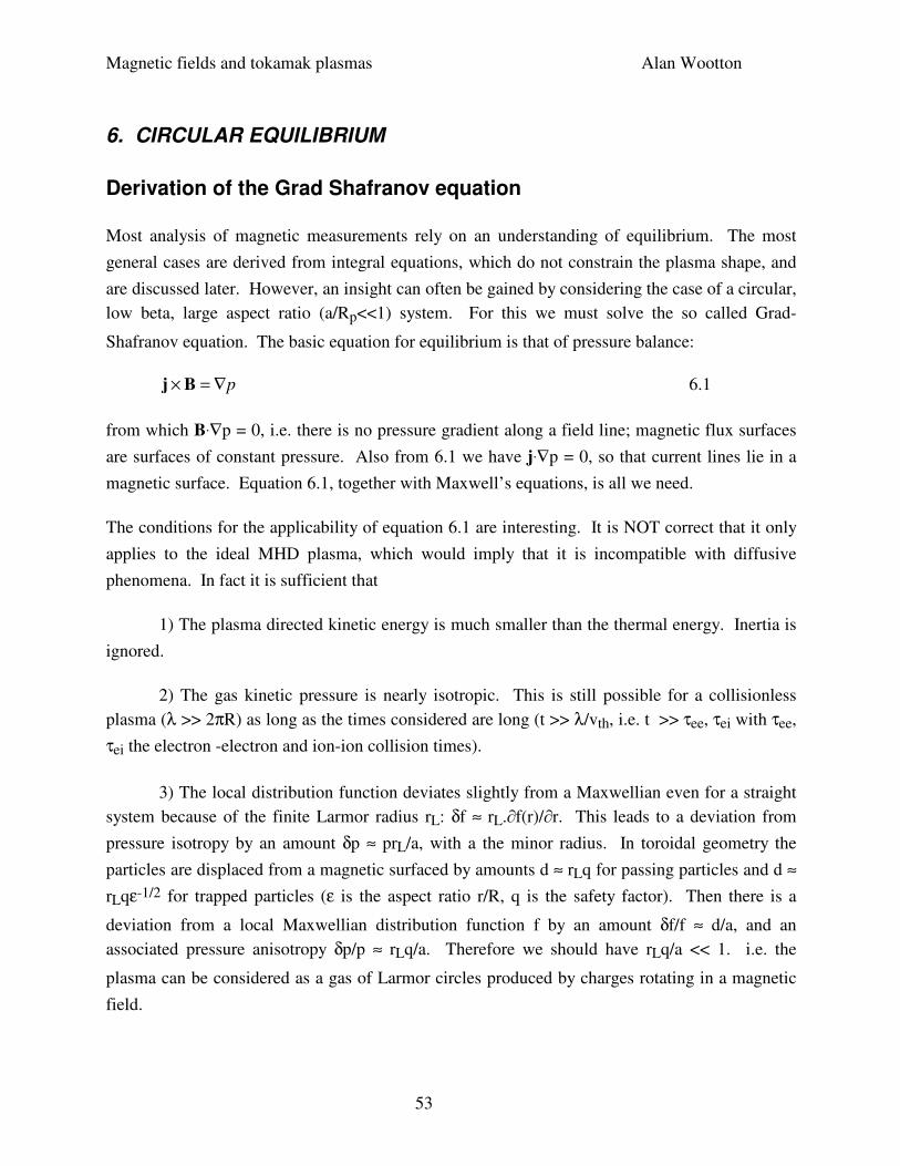
Magnetic fields and tokamak plasmas Alan Wootton
53
6. CIRCULAR EQUILIBRIUM
Derivation of the Grad Shafranov equation
Most analysis of magnetic measurements rely on an understanding of equilibrium. The most
general cases are derived from integral equations, which do not constrain the plasma shape, and
are discussed later. However, an insight can often be gained by considering the case of a circular,
low beta, large aspect ratio (a/Rp<<1) system. For this we must solve the so called Grad-
Shafranov equation. The basic equation for equilibrium is that of pressure balance:
j × B = ∇p 6.1
from which B.∇p = 0, i.e. there is no pressure gradient along a field line; magnetic flux surfaces
are surfaces of constant pressure. Also from 6.1 we have j.∇p = 0, so that current lines lie in a
magnetic surface. Equation 6.1, together with Maxwell’s equations, is all we need.
The conditions for the applicability of equation 6.1 are interesting. It is NOT correct that it only
applies to the ideal MHD plasma, which would imply that it is incompatible with diffusive
phenomena. In fact it is sufficient that
1) The plasma directed kinetic energy is much smaller than the thermal energy. Inertia is
ignored.
2) The gas kinetic pressure is nearly isotropic. This is still possible for a collisionless
plasma (λ >> 2πR) as long as the times considered are long (t >> λ/vth, i.e. t >> τee, τei with τee,
τei the electron -electron and ion-ion collision times).
3) The local distribution function deviates slightly from a Maxwellian even for a straight
system because of the finite Larmor radius rL: δf ≈ rL.∂f(r)/∂r. This leads to a deviation from
pressure isotropy by an amount δp ≈ prL/a, with a the minor radius. In toroidal geometry the
particles are displaced from a magnetic surfaced by amounts d ≈ rLq for passing particles and d ≈
rLqε-1/2 for trapped particles (ε is the aspect ratio r/R, q is the safety factor). Then there is a
deviation from a local Maxwellian distribution function f by an amount δf/f ≈ d/a, and an
associated pressure anisotropy δp/p ≈ rLq/a. Therefore we should have rLq/a << 1. i.e. the
plasma can be considered as a gas of Larmor circles produced by charges rotating in a magnetic
field.
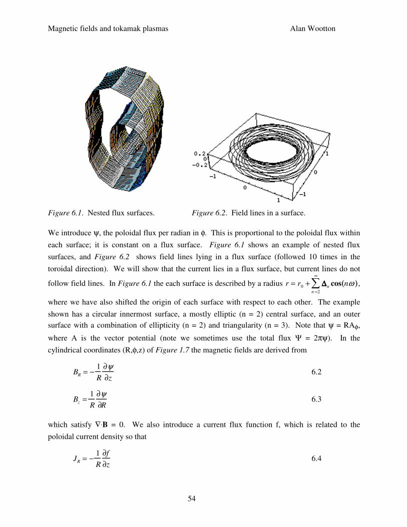
Magnetic fields and tokamak plasmas Alan Wootton
54
Figure 6.1. Nested flux surfaces. Figure 6.2. Field lines in a surface.
We introduce ψ, the poloidal flux per radian in φ. This is proportional to the poloidal flux within
each surface; it is constant on a flux surface. Figure 6.1 shows an example of nested flux
surfaces, and Figure 6.2 shows field lines lying in a flux surface (followed 10 times in the
toroidal direction). We will show that the current lies in a flux surface, but current lines do not
follow field lines. In Figure 6.1 the each surface is described by a radius r = r0 + ∆∆∆∆n cos nω( )n =2
∞
∑ ,
where we have also shifted the origin of each surface with respect to each other. The example
shown has a circular innermost surface, a mostly elliptic (n = 2) central surface, and an outer
surface with a combination of ellipticity (n = 2) and triangularity (n = 3). Note that ψ = RAφ,
where A is the vector potential (note we sometimes use the total flux Ψ = 2πψ). In the
cylindrical coordinates (R,φ,z) of Figure 1.7 the magnetic fields are derived from
BR = −1
R
∂ψ∂z
6.2
Bz =1
R
∂ψ∂R
6.3
which satisfy ∇.B = 0. We also introduce a current flux function f, which is related to the
poloidal current density so that
JR = −1
R
∂f
∂z 6.4
Magnetic fields and tokamak plasmas Alan Wootton
55
jz =1
R
∂f
∂R 6.5
Now Amperes law µ0j = ∇ x B gives
jR = −1
µ0
∂Bφ
∂z 6.6
jz =1
µ 0R
∂ RBφ( )∂R
6.7
so that, comparing Equation 6.4 with Equation 6.6, and Equation 6.5 with Equation 6.7, we have
µ 0 f = RBφ 6.8
That is, the function f includes the total current in the windings producing the toroidal field.
Since from Equation 6.1. j.∇p = 0, using Equations 6.4 and 6.5 for j gives (∂f/∂R)(∂p/∂z) -
(∂f/∂z)(∂p/∂R) = 0, or
∇f × ∇p = 0 6.9
Since p is a function of ψ, i.e. p = p(ψ), we must have f = f(ψ) as well.
Now we want to derive the basic equilibrium equation in terms of ψ. Write Equation 6.1 as
jp × eφ Bφ + jφ eφ × Bp = ∇p 6.10
where subscript p means poloidal and eφ is a unit vector in the φ direction. Now Equations 6.2.
and 6.3 can be written as
Bp =1
R∇ψ × eφ( ) 6.11
and Equations 6.4 and 6.5 can be written as
jp =1
R∇f × eφ( ) 6.12
Substituting 6.11. and 6.12 into 6.10, (remember eφ.∇ψ = eφ.∇f = 0) gives
−Bφ
R∇f +
jφ
R∇ψ = ∇p 6.13
Magnetic fields and tokamak plasmas Alan Wootton
56
Writing ∇f(ψ) = (df/dψ)∇ψ and ∇p(ψ) = (dp/dψ)∇ψ, and substituting into 6.13, gives
jφ = Rdp
dψ+ Bφ
df
dψ 6.14
or
jφ = Rdp
dψ+
µ0
Rf
df
dψ 6.15
The equilibrium conditions restrict the possible current distributions jφ in the plasma ; instead of
a two dimensional distribution jφ(R,z) a one dimensional one is obtained, depending on the two
profiles dp/dψ and fdf/dψ.
We can write jφ in terms of ψ using Amperes law, µ0j = ∇ x B. Substituting from Equations 6.2
and 6.3 for the components of B in the toroidal component jφ gives
−µ0 Rjφ = R∂
∂R
1
R
∂ψ∂R
+
∂2ψ∂z
2 6.16
Substituting for jφ from Equation 6.16 into Equation 6.15 finally gives the Grad Shafranov
equation:
R∂
∂R
1
R
∂ψ∂R
+
∂2ψ∂z
2 = −µ0 R2 dp
dψ− µ0
2f
df
dψ 6.17
In the local coordinates (θ,r,φ) of Figure 6.3, based on the plasma major radius (the geometric
center of the outermost circular surface) Rg this equation becomes:
1
r
∂∂r
r∂
∂r
+
1
r2
∂2
∂θ 2
ψ −
1
Rg + rcos θ( )( ) cos θ( ) ∂∂r
−sin θ( )
r
∂∂θ
ψ
= −µ 0 Rg + rcos θ( )( )2 dp
dψ− µ0
2 fdf
dψ
6.18
Note the ordering (θ,r,φ) in which the system is right handed. The poloidal angle θ is measured
from the outer equator, so that x = R + rcos θ( )( )cos φ( ), y = R + r cos θ( )( )sin φ( ), and
z = rsin θ( ). The metric coefficients are hθ = r , hr =1 and hφ = R + r cos θ( ) . If a new variable
θ1 = π − θ is defined, so θ1 is measured from the inner equator, then the system (r,θ1,φ) is also
right handed. We have mostly used this latter system.
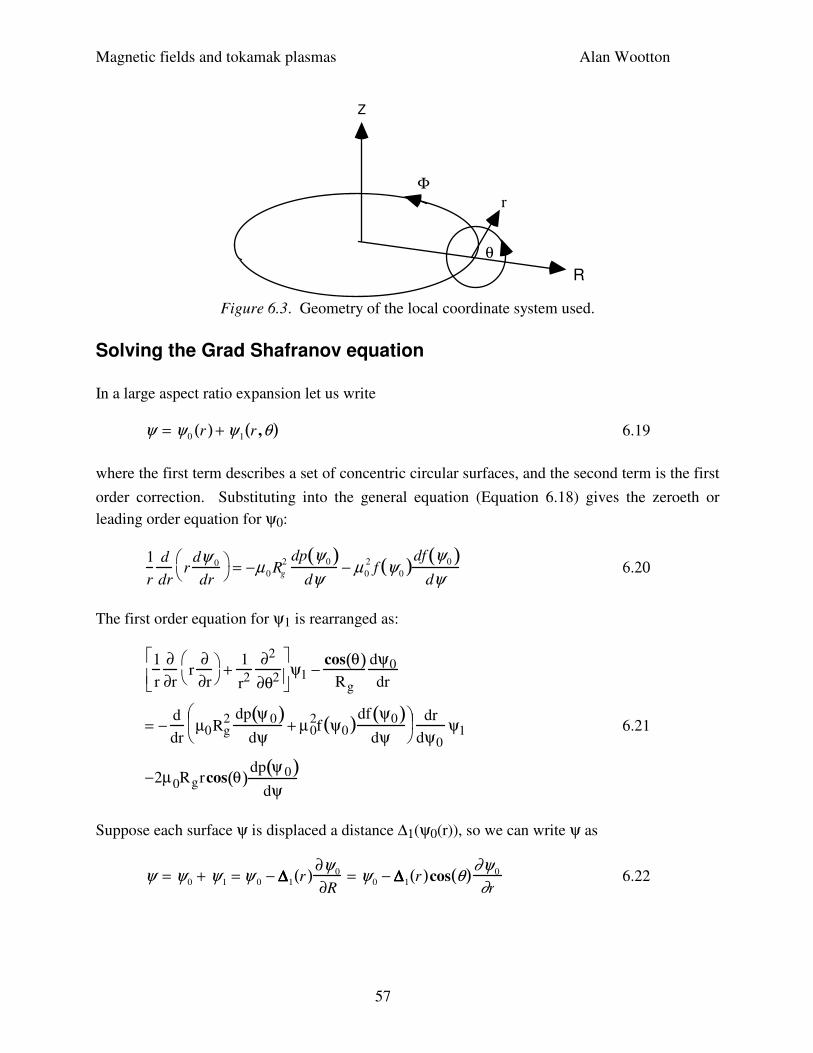
Magnetic fields and tokamak plasmas Alan Wootton
57
Φ
R
Z
r
θ
Figure 6.3. Geometry of the local coordinate system used.
Solving the Grad Shafranov equation
In a large aspect ratio expansion let us write
ψ = ψ0 r( ) + ψ1 r ,θ( ) 6.19
where the first term describes a set of concentric circular surfaces, and the second term is the first
order correction. Substituting into the general equation (Equation 6.18) gives the zeroeth or
leading order equation for ψ0:
1
r
d
drr
dψ 0
dr
= −µ 0 Rg
2 dp ψ0( )dψ
− µ0
2f ψ0( )df ψ0( )
dψ 6.20
The first order equation for ψ1 is rearranged as:
1
r
∂∂r
r∂∂r
+1
r2
∂2
∂θ2
ψ1 −
cos θ( )Rg
dψ0
dr
= −d
drµ0Rg
2 dp ψ 0( )dψ
+ µ02f ψ0( )df ψ0( )
dψ
dr
dψ0
ψ1
−2µ0Rgrcos θ( )dp ψ 0( )
dψ
6.21
Suppose each surface ψ is displaced a distance ∆1(ψ0(r)), so we can write ψ as
ψ = ψ0 + ψ1 = ψ 0 − ∆∆∆∆1 r( )∂ψ0
∂R= ψ0 − ∆∆∆∆1 r( )cos θ( )∂ψ0
∂r 6.22
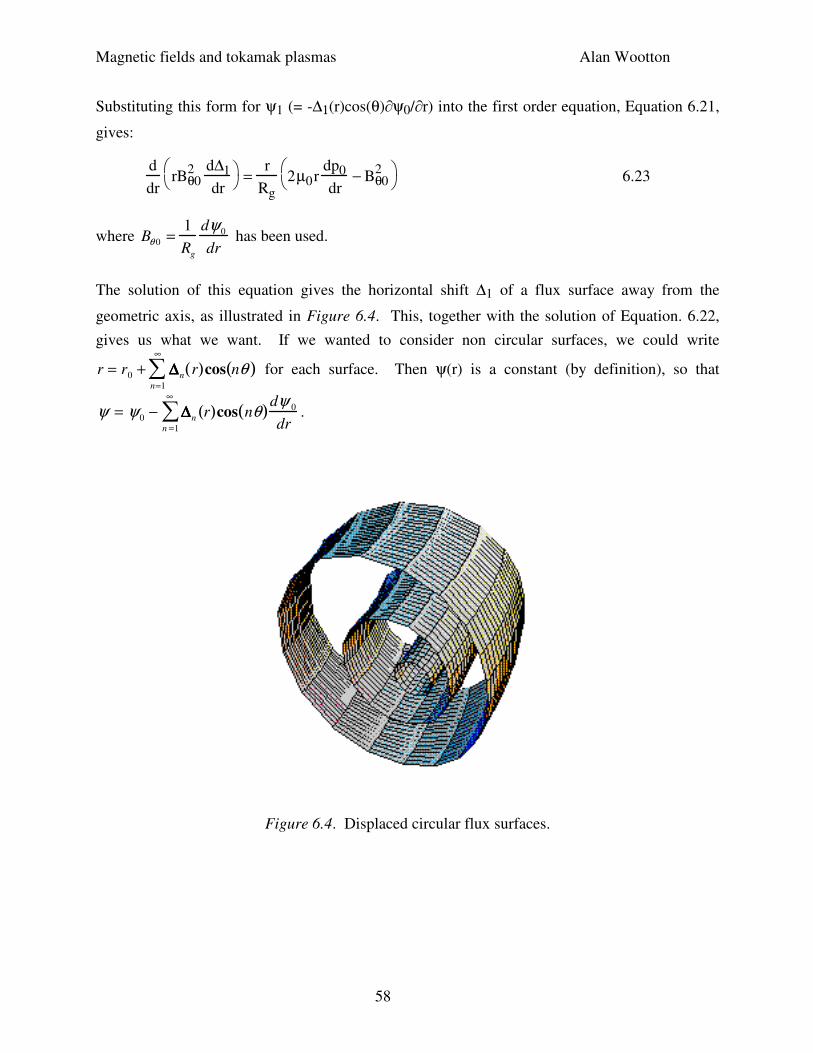
Magnetic fields and tokamak plasmas Alan Wootton
58
Substituting this form for ψ1 (= -∆1(r)cos(θ)∂ψ0/∂r) into the first order equation, Equation 6.21,
gives:
d
drrBθ0
2 d∆1
dr
=
r
Rg
2µ0rdp0
dr− Bθ0
2
6.23
where Bθ 0 =1
Rg
dψ0
dr has been used.
The solution of this equation gives the horizontal shift ∆1 of a flux surface away from the
geometric axis, as illustrated in Figure 6.4. This, together with the solution of Equation. 6.22,
gives us what we want. If we wanted to consider non circular surfaces, we could write
r = r0 + ∆∆∆∆n r( )cos nθ( )n=1
∞
∑ for each surface. Then ψ(r) is a constant (by definition), so that
ψ = ψ0 − ∆∆∆∆n r( )cos nθ( )n =1
∞
∑dψ 0
dr.
Figure 6.4. Displaced circular flux surfaces.
Magnetic fields and tokamak plasmas Alan Wootton
59
The poloidal field at the plasma edge
To continue, we need an expression for the boundary field Bθ(a) from the plasma equilibrium.
We will ultimately use this to match the external and internal solutions at the plasma boundary r
= a, where Bτ (= Bθ for a circular plasma) must be continuous. Now
Bθ =1
R
dψdr
=1
Rg + r cosθ( )dψdr
6.24
Using Equation 6.22, with ∆1(a) = 0, gives
Bθ a( ) = Bθ 0 a( ) 1 −a
Rg
+d∆∆∆∆1
dr
a
cos θ( )
6.25
with Bθ0(a) the zero order poloidal field at the boundary. Now we need to find an expression for
(d∆1/dr)a in Equation 6.25. Integrating Equation 6.23 (with the condition d∆1/dr = 0 at r = 0)
gives the displacement of the magnetic surfaces for the zero order pressure distribution p0(r) and
zero order poloidal field Bθo(r):
d∆∆∆∆1
dr=
2µ0
rRg Bθ 0
2 r2p0 − 2 p0 +
Bθ 0
2
2µ0
rdr
0
r
∫
6.26
By defining (we will be more careful with definitions later)
βI =8π
µ0Ip
2 pdSφSφp
∫ =4µ 0
a2Bθ 0
2a( )
p0 rdr0
a
∫ 6.27
for our circular case, and
li =4
µ 0RgIp
2
Bp
2
2µ0
dV =V p
∫4µ 0
a2Bθ0
2a( )
Bθ2
2µ00
a
∫ rdr 6.28
where Bp is the poloidal field, Spφ the plasma cross section in a poloidal plane, and Vp the
plasma volume, for our circular case we obtain
d∆1
dr
a= −
a
Rg
βI +li
2
6.29
Now we can substitute Equation 6.29 into 6.25 and obtain
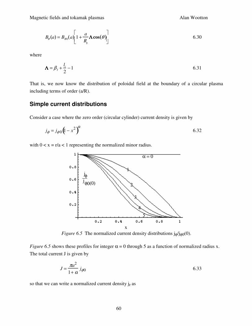
Magnetic fields and tokamak plasmas Alan Wootton
60
Bθ a( ) = Bθ 0 a( ) 1 +a
Rg
ΛΛΛΛ cos θ( )
6.30
where
ΛΛΛΛ = β I +li
2−1 6.31
That is, we now know the distribution of poloidal field at the boundary of a circular plasma
including terms of order (a/R).
Simple current distributions
Consider a case where the zero order (circular cylinder) current density is given by
jφ = jφ 0 1 − x2( )α 6.32
with 0 < x = r/a < 1 representing the normalized minor radius.
α = 0
1
2
3
4
5
x
jφ__jφ0(0)
Figure 6.5 The normalized current density distributions jφ/jφ0(0).
Figure 6.5 shows these profiles for integer α = 0 through 5 as a function of normalized radius x.
The total current J is given by
J =πa2
1+ αjφ0 6.33
so that we can write a normalized current density jr as
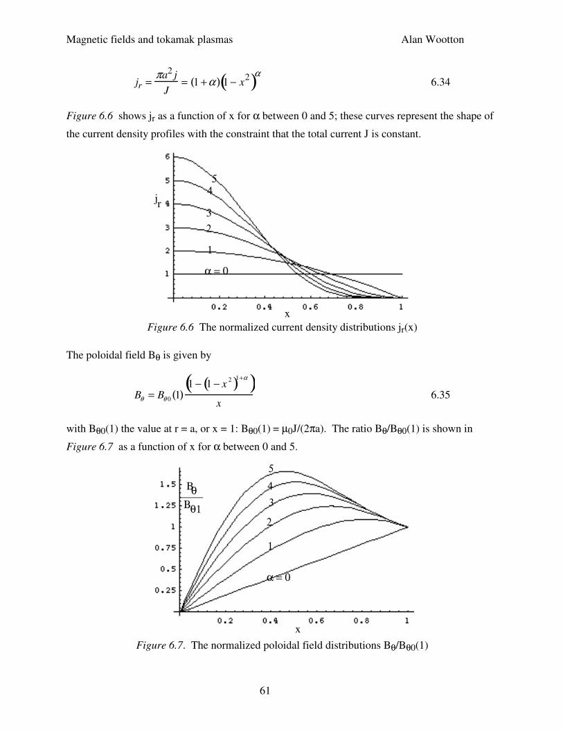
Magnetic fields and tokamak plasmas Alan Wootton
61
jr =πa2 j
J= 1 +α( ) 1 − x
2( )α 6.34
Figure 6.6 shows jr as a function of x for α between 0 and 5; these curves represent the shape of
the current density profiles with the constraint that the total current J is constant.
α = 0
1
23
45
x
jr
Figure 6.6 The normalized current density distributions jr(x)
The poloidal field Bθ is given by
Bθ = Bθ 0 1( )1 − 1 − x
2( )1+α( )x
6.35
with Bθ0(1) the value at r = a, or x = 1: Bθ0(1) = µ0J/(2πa). The ratio Bθ/Bθ0(1) is shown in
Figure 6.7 as a function of x for α between 0 and 5.
α = 0
1
2
3
4
5
x
Bθ____Βθ1
Figure 6.7. The normalized poloidal field distributions Bθ/Bθ0(1)
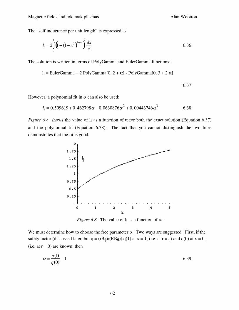
Magnetic fields and tokamak plasmas Alan Wootton
62
The “self inductance per unit length” is expressed as
li = 2 1 − 1 − x2( )1+α( )
0
1
∫2
dx
x 6.36
The solution is written in terms of PolyGamma and EulerGamma functions:
li = EulerGamma + 2 PolyGamma[0, 2 + α] - PolyGamma[0, 3 + 2 α]
6.37
However, a polynomial fit in α can also be used:
li = 0.509619 + 0 .462798α − 0.0630876α 2 + 0. 00443746α3 6.38
Figure 6.8 shows the value of li as a function of α for both the exact solution (Equation 6.37)
and the polynomial fit (Equation 6.38). The fact that you cannot distinguish the two lines
demonstrates that the fit is good.
α
li
Figure 6.8. The value of li as a function of α.
We must determine how to choose the free parameter α. Two ways are suggested. First, if the
safety factor (discussed later, but q = (rBφ)/(RBθ)) q(1) at x = 1, (i.e. at r = a) and q(0) at x = 0,
(i.e. at r = 0) are known, then
α =q(1)
q(0)− 1 6.39
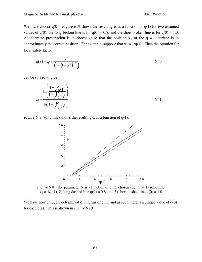
Magnetic fields and tokamak plasmas Alan Wootton
63
We must choose q(0). Figure 6 .9 shows the resulting α as a function of q(1) for two assumed
values of q(0): the long broken line is for q(0) = 0.8, and the short broken line is for q(0) = 1.0.
An alternate prescription is to choose α so that the position x1 of the q = 1 surface is in
approximately the correct position. For example, suppose that x1 = 1/q(1). Then the equation for
local safety factor
q x( ) = q 1( )x2
1− 1 − x2( )1+α( ) 6.40
can be solved to give
α =
ln1 − 1
q(1)
1 − 1q(1)
2
ln 1 − 1q(1)2
6.41
Figure 6 .9 (solid line) shows the resulting α as a function of q(1).
α
q(1) Figure 6.9. The parameter α as a function of q(1), chosen such that 1) solid line:
x1 = 1/q(1), 2) long dashed line q(0) = 0.8, and 3) short dashed line q(0) = 1.0.
We have now uniquely determined α in terms of q(1), and as such there is a unique value of q(0)
for each q(a). This is shown in Figure 6.10
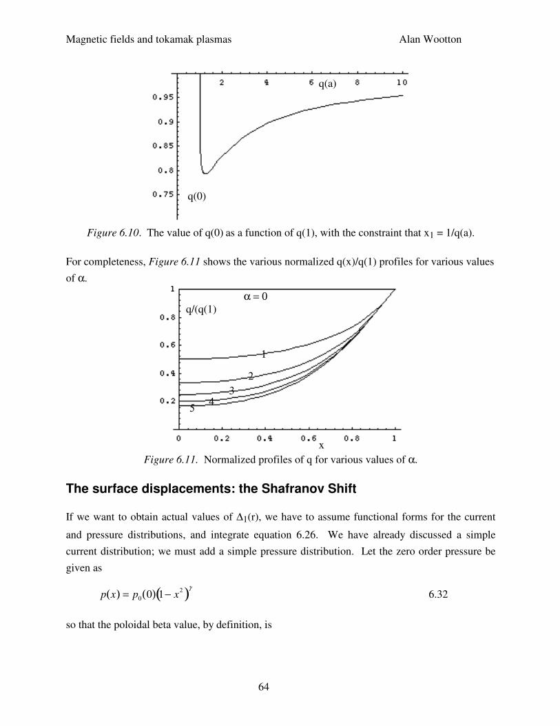
Magnetic fields and tokamak plasmas Alan Wootton
64
q(0)
q(a)
Figure 6.10. The value of q(0) as a function of q(1), with the constraint that x1 = 1/q(a).
For completeness, Figure 6.11 shows the various normalized q(x)/q(1) profiles for various values
of α.
q/(q(1)
x
α = 0
1
23
45
Figure 6.11. Normalized profiles of q for various values of α.
The surface displacements: the Shafranov Shift
If we want to obtain actual values of ∆1(r), we have to assume functional forms for the current
and pressure distributions, and integrate equation 6.26. We have already discussed a simple
current distribution; we must add a simple pressure distribution. Let the zero order pressure be
given as
p x( ) = p0 0( ) 1− x2( )γ
6.32
so that the poloidal beta value, by definition, is
Magnetic fields and tokamak plasmas Alan Wootton
65
βI =2µ0 p0 0( )
1+ γ( )Bθ 0
21( )
6.42
Now we can use the normalization x = r/a in equation 6.26 to obtain an expression for the surface
displacement:
d∆∆∆∆1
dx= −
εa
2
2x
1 − 1− x2( )1+ α( )2
βI γ +1( )x 21− x
2( )γ− βI 1 − 1 − x
2( )γ +1( )− 1 − 1 − x2( )1+α( )
2 dx
x0
x
∫
6.43
Where ε = a/Rg. The Shafranov Shift is defined as the distance between the magnetic and
geometric axis: ∆s = ∆1(1). Using a power series expansion for ∆1(x) up to terms x6 a general
expression can be derived:
∆∆∆∆ s =εa
2
1 + 2α9
+ α 2
72
4+
βI γ γ +1( )4 1 + α( )2
2 +11α
9+
5α 2
18+
γ − 1( ) γ − 6( )6
−4α γ −1( )
9
6.44
For the simple case of a flat current profile (α = 0, li = 0.5) and a parabolic pressure profile (γ =
1) we obtain
∆∆∆∆ s =εa
2βI +
li
2
6.45
Matching vacuum and plasma solutions
Returning to the field outside the plasma, we must match the vacuum field to the solution for
Bθ(a). The vacuum field is given by the solution to (∇xB)φ = 0. Expressing BR and Bz in terms
of ψ (Equations 6.2 and 6.3), (∇xB)φ has the form of the LHS of Equation 6.18. This has a
solution of the form (for r << Rg); remember we are outside the plasma:
Ψ = 2πψ r ,θ( ) = µ0RgIp ln8Rg
r
− 2
+µ0Ip
2r ln
8Rg
r
−1
+
C1
r+ C2r
cos θ( )
6.46
Magnetic fields and tokamak plasmas Alan Wootton
66
where the constants C1 and C2 are given by the boundary conditions (B.n) = 0 at the plasma
surface (Br(a) = 0) and the continuity of tangential field at the plasma surface. At infinity ψ takes
the form C2rcos(θ), i.e. this represents the part of ψ from the external sources. The first term on
the RHS is the flux from a filament. Substituting 6.46 into 6.24 gives an expression for Bθ(a),
which is matched to the plasma solution equation 6.30 by taking
C1
a2 − C2 = ln
8Rg
a
+ 2ΛΛΛΛ 6.47
Now since Br =−1
rRg
∂ψ∂θ
the requirement Br(a) = 0 means that the coefficient of cos(θ) in 6.46 is
zero at r = a. Therefore we obtain
C1 = a2 ΛΛΛΛ + 0.5( ) 6.48
C2 = − ln8Rg
2
+ ΛΛΛΛ − 0.5 6.49
Thus we finally obtain an expression for the flux outside the plasma r > a:
ψ =µ0 RgI p
2πln
8Rg
r
− 2
−µ 0rI p
4π1 − a
2
r2
ΛΛΛΛ + 1
2
+ ln
r
a
cos θ( )
6.50
The field components are given by
Bθ =1
R
∂ψ∂r
, Br = −1
Rgr
∂ψ∂θ
6.51
i.e.
Bθ(r,θ) = −
µ0Ip
2πr−
µ0Ip
2πRg
1 +ap
2
r2
Λ +
1
2
+ ln
r
ap
−1
cos θ( )
6.52
Br r,θ( )= −µ0Ip
4πRg
1 −ap
2
r2
Λ +
1
2
+ ln
r
ap
sin θ( ) 6.53
Magnetic fields and tokamak plasmas Alan Wootton
67
We can also separate the total flux ψ into external (ψe) and plasma (ψp) parts. At large r, the
expression (ln(8Rg/r) -2) really approximates an expression which goes to zero. Therefore at
large r we have
ψ e = −µ 0I p
4πln
8Rg
a
+ ΛΛΛΛ −
1
2
r cos θ( ) 6.54
leaving
ψ p =µ0 RgIp
2πln
8Rg
r
− 2
−µ 0rI p
4π− ln
8Rg
r
+1 − a
r
2
ΛΛΛΛ + 1
2
cos θ( )
6.55
i.e. the external field at the geometric center (R = Rg) has a component
Bz =1
R
∂ψ e
∂R= −
µ 0 Ip
4πRg
ln8Rg
a
+ ΛΛΛΛ −
1
2
6.56
This is the component of the field which must be produced by external conductors to maintain a
tokamak equilibrium.
Figure 6.12 shows contours of the poloidal flux for a plasma with geometric center 0.06 m
outside the coordinate center, minor radius ap = 0.265 m, and Λ = 2. At the inner equator an X
point appears, where ∂ψ/∂R = 0. At this point the external vertical field and the poloidal field
from the plasma cancel, so that Bz (= -Bθ) = 0. The flux surface through this point is called the
separatrix. This X point approaches the plasma surface as βI increases. As this happens the
surfaces are strongly distorted from circular, and the above equations starts break down. Figure
6.13 shows the poloidal flux ψ =Ψ/(2π) in the plane z = 0 for a plasma with minor radius ap =
0.2m, a major geometric radius Rg = 1m, current I = 1/µ0, and Λ = 2. The external source
(vertical field) and plasma components are shown separately. Figure 6.14 shows the minor radial
(Br) and poloidal (Bθ) field components for this plasma, on a circular contour concentric with the
plasma minor radius.
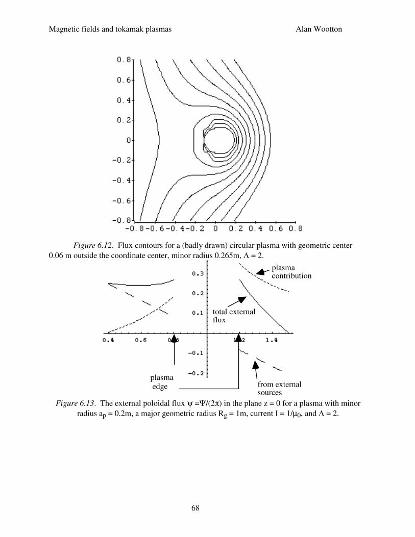
Magnetic fields and tokamak plasmas Alan Wootton
68
Figure 6.12. Flux contours for a (badly drawn) circular plasma with geometric center
0.06 m outside the coordinate center, minor radius 0.265m, Λ = 2.
from external sources
total external flux
plasma contribution
plasmaedge
Figure 6.13. The external poloidal flux ψ =Ψ/(2π) in the plane z = 0 for a plasma with minor
radius ap = 0.2m, a major geometric radius Rg = 1m, current I = 1/µ0, and Λ = 2.
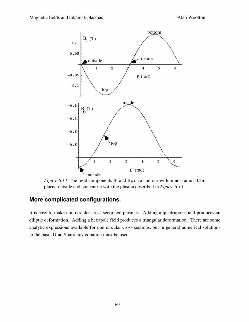
Magnetic fields and tokamak plasmas Alan Wootton
69
Br (T)
θ (rad)
outside
top
inside
bottom
B (T)θ
θ (rad)outside
top
inside
Figure 6.14. The field components Br and Bθ on a contour with minor radius 0.3m
placed outside and concentric with the plasma described in Figure 6.13.
More complicated configurations.
It is easy to make non circular cross sectioned plasmas. Adding a quadrupole field produces an
elliptic deformation. Adding a hexapole field produces a triangular deformation. There are some
analytic expressions available for non circular cross sections, but in general numerical solutions
to the basic Grad Shafranov equation must be used.
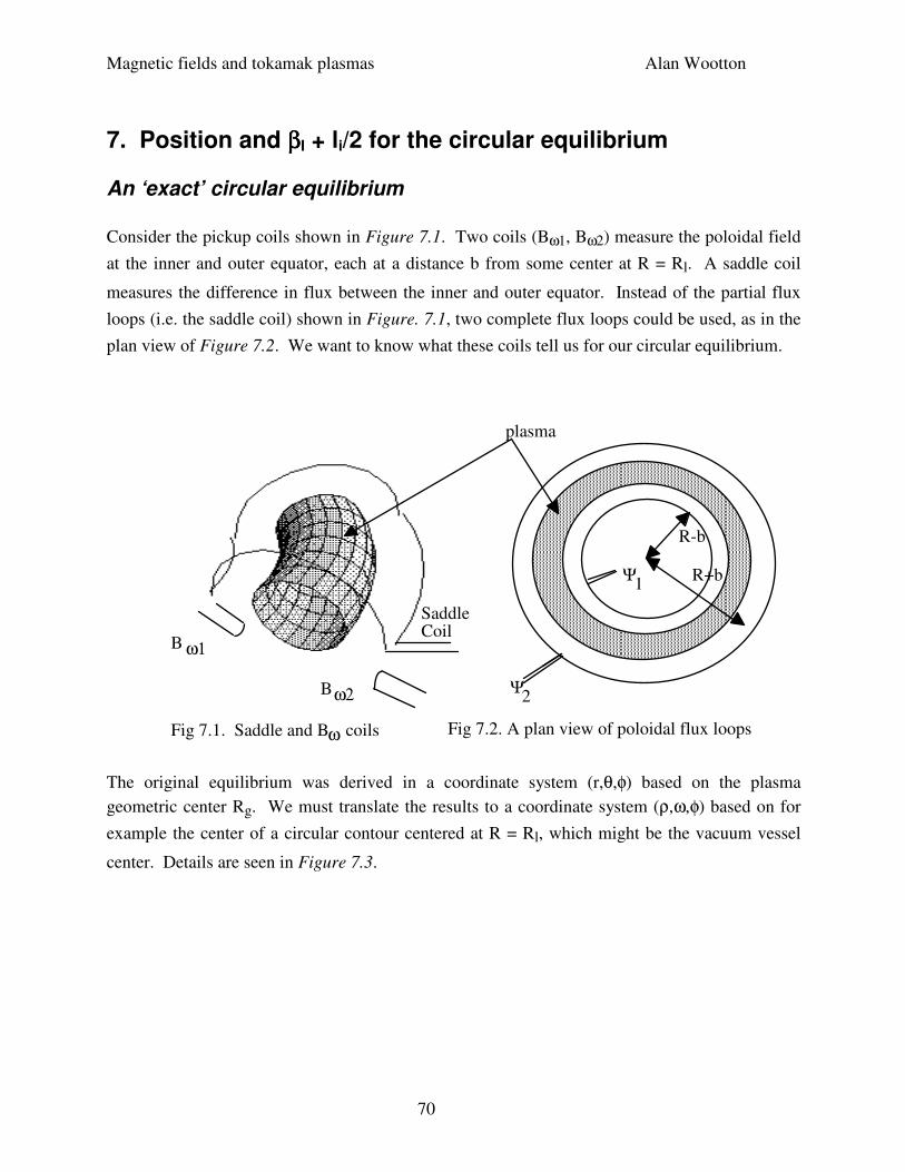
Magnetic fields and tokamak plasmas Alan Wootton
70
7. Position and ββββI + li/2 for the circular equilibrium
An ‘exact’ circular equilibrium
Consider the pickup coils shown in Figure 7.1. Two coils (Bω1, Bω2) measure the poloidal field
at the inner and outer equator, each at a distance b from some center at R = Rl. A saddle coil
measures the difference in flux between the inner and outer equator. Instead of the partial flux
loops (i.e. the saddle coil) shown in Figure. 7.1, two complete flux loops could be used, as in the
plan view of Figure 7.2. We want to know what these coils tell us for our circular equilibrium.
Saddle Coil
ω1
ω2
Fig 7.1. Saddle and Bω coils
R-b
R+bΨ
Ψ
plasma
B
B
Fig 7.2. A plan view of poloidal flux loops
1
2
The original equilibrium was derived in a coordinate system (r,θ,φ) based on the plasma
geometric center Rg. We must translate the results to a coordinate system (ρ,ω,φ) based on for
example the center of a circular contour centered at R = Rl, which might be the vacuum vessel
center. Details are seen in Figure 7.3.
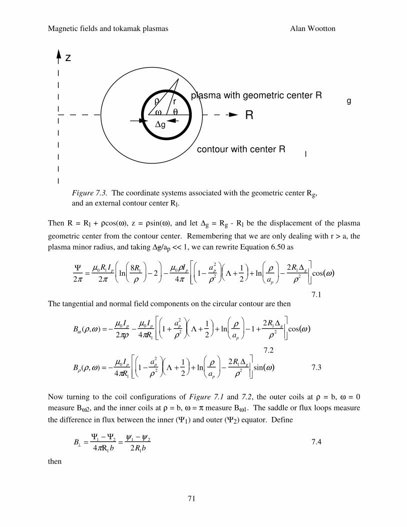
Magnetic fields and tokamak plasmas Alan Wootton
71
ρω
rθ
contour with center Rl
plasma with geometric center Rg
∆g
z
R
Figure 7.3. The coordinate systems associated with the geometric center Rg,
and an external contour center Rl.
Then R = Rl + ρcos(ω), z = ρsin(ω), and let ∆g = Rg - Rl be the displacement of the plasma
geometric center from the contour center. Remembering that we are only dealing with r > a, the
plasma minor radius, and taking ∆g/ap << 1, we can rewrite Equation 6.50 as
Ψ2π
=µ0 Rl I p
2πln
8Rl
ρ
− 2
−
µ0 ρIp
4π1−
ap
2
ρ2
Λ +
1
2
+ ln
ρap
−
2Rl ∆g
ρ2
cos ω( )
7.1
The tangential and normal field components on the circular contour are then
Bω (ρ,ω ) = −µ0 Ip
2πρ−
µ0 Ip
4πRl
1 +ap
2
ρ2
Λ +
1
2
+ ln
ρap
−1 +
2Rl ∆g
ρ 2
cos ω( )
7.2
Bρ (ρ,ω) = −µ0 Ip
4πRl
1 −ap
2
ρ 2
Λ +
1
2
+ ln
ρap
−
2Rl ∆g
ρ2
sin ω( ) 7.3
Now turning to the coil configurations of Figure 7.1 and 7.2, the outer coils at ρ = b, ω = 0
measure Bω2, and the inner coils at ρ = b, ω = π measure Bω1. The saddle or flux loops measure
the difference in flux between the inner (Ψ1) and outer (Ψ2) equator. Define
B⊥ =Ψ1 − Ψ2
4πRl b=
ψ1 −ψ 2
2Rlb 7.4
then
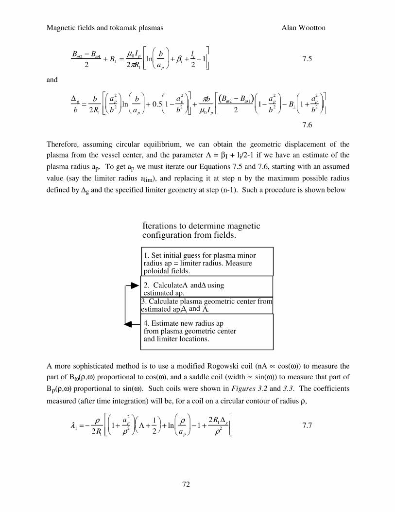
Magnetic fields and tokamak plasmas Alan Wootton
72
Bω 2 − Bω1
2+ B⊥ =
µ0 Ip
2πRl
lnb
ap
+ βl +
li
2−1
7.5
and
∆ g
b=
b
2Rl
ap
2
b2
ln
b
ap
+ 0.5 1 −
a p
2
b2
+πb
µ0 I p
Bω 2 − Bω 1( )2
1−ap
2
b2
− B⊥ 1 +
ap
2
b2
7.6
Therefore, assuming circular equilibrium, we can obtain the geometric displacement of the
plasma from the vessel center, and the parameter Λ = βI + li/2-1 if we have an estimate of the
plasma radius ap. To get ap we must iterate our Equations 7.5 and 7.6, starting with an assumed
value (say the limiter radius alim), and replacing it at step n by the maximum possible radius
defined by ∆g and the specified limiter geometry at step (n-1). Such a procedure is shown below
3. Calculate plasma geometric center from estimated ap,
4. Estimate new radius ap from plasma geometric center and limiter locations.
1. Set initial guess for plasma minor radius ap = limiter radius. Measure poloidal fields.
2. Calculate and using estimated ap.
Λ ∆
∆ Λ, and .
Iterations to determine magnetic configuration from fields.
A more sophisticated method is to use a modified Rogowski coil (nA ∝ cos(ω)) to measure the
part of Bω(ρ,ω) proportional to cos(ω), and a saddle coil (width ∝ sin(ω)) to measure that part of
Bρ(ρ,ω) proportional to sin(ω). Such coils were shown in Figures 3.2 and 3.3. The coefficients
measured (after time integration) will be, for a coil on a circular contour of radius ρ,
λ1 = −ρ
2Rl
1+a p
2
ρ2
Λ +
1
2
+ ln
ρap
−1 +
2Rl ∆g
ρ2
7.7
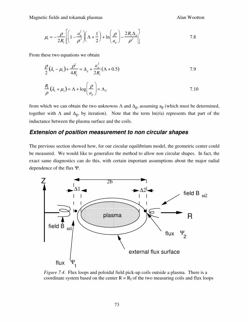
Magnetic fields and tokamak plasmas Alan Wootton
73
µ1 = −ρ
2Rl
1 −ap
2
ρ 2
Λ +
1
2
+ ln
ρap
−
2Rl ∆g
ρ 2
7.8
From these two equations we obtain
ρ2
λ1 − µ1( )+ρ2
4Rg
= ∆g +ap
2
2Rl
Λ + 0.5( ) 7.9
Rl
ρλ1 + µ1( ) = Λ + log
ρap
= ΛT 7.10
from which we can obtain the two unknowns Λ and ∆g, assuming ap (which must be determined,
together with Λ and ∆g, by iteration). Note that the term ln(r/a) represents that part of the
inductance between the plasma surface and the coils.
Extension of position measurement to non circular shapes
The previous section showed how, for our circular equilibrium model, the geometric center could
be measured. We would like to generalize the method to allow non circular shapes. In fact, the
exact same diagnostics can do this, with certain important assumptions about the major radial
dependence of the flux Ψ.
• •
flux Ψ1
field B ω1
plasma
external flux surface
R
Z
flux Ψ2
field B ω2∆2∆1
2b
Figure 7.4. Flux loops and poloidal field pick-up coils outside a plasma. There is a
coordinate system based on the center R = Rl of the two measuring coils and flux loops
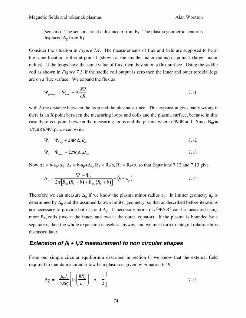
Magnetic fields and tokamak plasmas Alan Wootton
74
(sensors). The sensors are at a distance b from Rl. The plasma geometric center is
displaced ∆g from Rl.
Consider the situation in Figure 7.4. The measurements of flux and field are supposed to be at
the same location, either at point 1 (shown at the smaller major radius) or point 2 (larger major
radius). If the loops have the same value of flux, then they sit on a flux surface. Using the saddle
coil as shown in Figure 7.1, if the saddle coil output is zero then the inner and outer toroidal legs
are on a flux surface. We expand the flux as
Ψplasma = Ψloop + ∆∂Ψ∂R
7.11
with ∆ the distance between the loop and the plasma surface. This expansion goes badly wrong if
there is an X point between the measuring loops and coils and the plasma surface, because in this
case there is a point between the measuring loops and the plasma where ∂Ψ/dR = 0. Since Bω =
1/(2πR)∂Ψ/∂ρ, we can write
Ψ1 = Ψloop + 2πR1∆1Bω1 7.12
Ψ2 = Ψloop + 2πR2∆ 2Bω 2 7.13
Now ∆2 = b-ap-∆g, ∆1 = b-ap+∆g, R1 = Rl-b, R2 = Rl+b, so that Equations 7.12 and 7.13 give
∆ g =Ψ1 − Ψ2
2π Bω1 Rl − b( ) + Bω 2 Rl + b( )[ ]− b − ap( ) 7.14
Therefore we can measure ∆g if we know the plasma minor radius ap. In limiter geometry ap is
determined by ∆g and the assumed known limiter geometry, so that as described before iterations
are necessary to provide both ap and ∆g. If necessary terms in ∂2Ψ/∂R2 can be measured using
more Bω coils (two at the inner, and two at the outer, equator). If the plasma is bounded by a
separatrix, then the whole expansion is useless anyway, and we must turn to integral relationships
discussed later.
Extension of ββββI + li/2 measurement to non circular shapes
From our simple circular equilibrium described in section 6, we know that the external field
required to maintain a circular low beta plasma is given by Equation 6.49:
BZ = −µ0 Ip
4πRg
ln8Rg
a p
+ Λ −
1
2
7.15
Magnetic fields and tokamak plasmas Alan Wootton
75
Therefore if we know all the currents in the external conductors, the plasma current, minor radius
and major radius, we can calculate BZ at the geometric axis R = Rg, and obtain a value for Λ = βI
+ li/2 -1. The result (Equation 7.15) has been found by numerical simulation to be accurate even
for non circular discharges. Therefore if we can calculate the maintaining field, and know the
plasma minor radius and geometric center, we can calculate βI + li/2. It becomes difficult to
calculate the maintaining field if we have an iron core present; we will discuss this later.
However, there are more general techniques which do not explicitly require this calculation of
fields from currents, and we also discuss these later.
Non-circular contours.
So far we have only considered poloidal field measurements which can be made on a circular
contour. In many cases the simplest contour to use is that of the vacuum vessel, which is often
non circular. What do we do then? In section 3 we discussed how fields on a rectangle can be
characterized, and suggested that coils wound to measure “moments” might be useful.
Specifically, we discussed modified Rogowski coils which would measure
s p ,τ = f p Bτdll
∫ 7.16
and saddle coils which would measure
s p ,n = f pBndll
∫ 7.17
where the functions fp were taken to be the pth power of a vector radius on the contour l. The
geometry is re drawn in Figure 7.5.
Magnetic fields and tokamak plasmas Alan Wootton
76
η
ξ
Rl
z
R
Contour l
plasma
Figure 7.5. Geometry used for a non-circular contour.
An analogy with our cosinusoidally wound Rogowski coil and sinusoidally wound saddle coil
would be a modified Rogowski coil measuring the first symmetric (in vertical position) moment
s1,τ = ξBτdll
∫ 7.18
and a saddle coil measuring the first asymmetric (in vertical position) moment
λ1 = −ρ
2Rl
1+a p
2
ρ2
Λ +
1
2
+ ln
ρap
−1 +
2Rl ∆g
ρ2
7.19
To interpret what these coils will measure, we can write an equation for the components Bτ and
Bn on our chosen contour (for a rectangular contour they will be either Bη or Bξ). Because the
only variables in the equations for an assumed circular equilibrium are the geometric
displacement ∆g, Λ and minor radius ap, we must be able to derive expressions for the measured
coil outputs s1,τ and s1,n in terms of these variables. For example, if our contour is a square of
half height and half width a, centered at R = Rl, we must find
s1,τ = s1, τ Ip ,ΛΛΛΛ,∆∆∆∆ g, ap , a, Rl( ) 7.20
s1,n = s1,n Ip, ΛΛΛΛ,∆∆∆∆g , ap ,a, Rl( ) 7.21
Magnetic fields and tokamak plasmas Alan Wootton
77
In principle we can then solve Equations 7.20 and 7.21 to give expressions for the required Λ
and ∆g. Iterations will be necessary because we will find ap entering the final results, which itself
is only determined once ∆g is known.
It may be that the particular geometry of the contour precludes performing the analytic integrals
(Equations 7.18 and 7.19, using the analytical representation for the equilibrium fields outside a
circular plasma). In this case the problem must be solved numerically. Equations 7.18 and 7.19
are solved numerically for many different ∆g, Λ, and ap (we assume the contour geometry does
not change!) A regression analysis is then performed, in which solutions of the form
ΛΛΛΛ = fs1n
Ip
,s1τ
Ip
,ap ,contourgeometry
7.22
∆∆∆∆ g = fs1n
Ip
,s1τ
Ip
,ap ,contourgeometry
7.23
are sought.
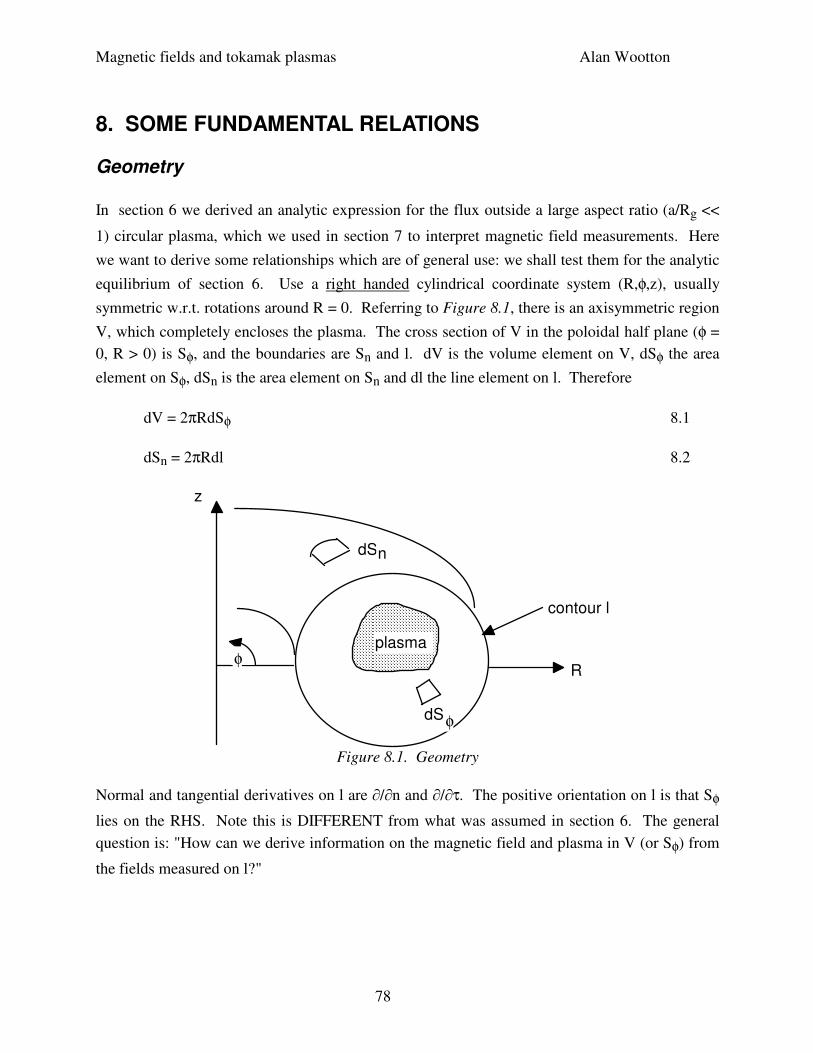
Magnetic fields and tokamak plasmas Alan Wootton
78
8. SOME FUNDAMENTAL RELATIONS
Geometry
In section 6 we derived an analytic expression for the flux outside a large aspect ratio (a/Rg <<
1) circular plasma, which we used in section 7 to interpret magnetic field measurements. Here
we want to derive some relationships which are of general use: we shall test them for the analytic
equilibrium of section 6. Use a right handed cylindrical coordinate system (R,φ,z), usually
symmetric w.r.t. rotations around R = 0. Referring to Figure 8.1, there is an axisymmetric region
V, which completely encloses the plasma. The cross section of V in the poloidal half plane (φ =
0, R > 0) is Sφ, and the boundaries are Sn and l. dV is the volume element on V, dSφ the area
element on Sφ, dSn is the area element on Sn and dl the line element on l. Therefore
dV = 2πRdSφ 8.1
dSn = 2πRdl 8.2
dSφ
plasma
dSn
R
z
φ
contour l
Figure 8.1. Geometry
Normal and tangential derivatives on l are ∂/∂n and ∂/∂τ. The positive orientation on l is that Sφ
lies on the RHS. Note this is DIFFERENT from what was assumed in section 6. The general
question is: "How can we derive information on the magnetic field and plasma in V (or Sφ) from
the fields measured on l?"
Magnetic fields and tokamak plasmas Alan Wootton
79
Field representation
We shall try and be as general as possible. First we quickly re-derive the equilibrium equation.
For the case of axisymmetry, we discussed in section 6 the description of the fields using the
form
Ψ2π
=µ0 Rl I p
2πln
8Rl
ρ
− 2
−
µ0 ρIp
4π1−
ap
2
ρ2
Λ +
1
2
+ ln
ρap
−
2Rl ∆g
ρ2
cos ω( )
8.3
where
F = RBφ = µ f 8.4
and ψ= RAφ
From ∇xH = j, we can also write
j = −1
µL
*ψ∇φ + ∇F
µ
× ∇φ 8.5
where the operator L* is defined for axisymmetric scalar fields as
L*ψ = µR
2∇ •∇ψµR
2
8.6
The operator L* satisfies the equation
L*ψ = −µRjφ 8.7.
For uniform permeability µ = µ0 we have L* reducing to the operator ∆*:
∆∆∆∆*ψ = R2∇ •
∇ψR
2
= R
∂∂R
1
R
∂ψ∂R
+
∂2ψ∂z
2 ∆ 8.8
That is, ∆* is the operator on the LHS of the Grad Shafranov equation. We also introduce the
operator L:
Lψ =1
µ∇ • µ∇ψ( ) 8.9
Magnetic fields and tokamak plasmas Alan Wootton
80
which reduces to the Laplacian ∆ for uniform permeability. In a current free region we can use
the representation H = ∇g, and ∇.B = 0 is then equivalent to Lg = 0.
Identities
Now we turn to some identities. Green's first identity for L* is:
1
µRSφ
∫ ψL*ΘΘΘΘdSφ =
1
µRl
∫ ψ∂ΘΘΘΘ∂n
dl −1
µRSφ
∫ ∇ψ • ∇ΘΘΘΘdSφ 8.10
Green's second identity (Green's theorem) is:
1
µRSφ
∫ ψL*ΘΘΘΘ − ΘΘΘΘL
*ψ( )dSφ =1
µRl
∫ ψ∂ΘΘΘΘ∂n
− ΘΘΘΘ∂ψ∂n
dl 8.11
Both of these are derived by applying the divergence theorem to appropriate expression on V. In
particular see Smythe, static and dynamic electricity, page 53 eqn. 3.06(2) for a derivation of
Green’s theorem, which is, for scalars A, B and E,
A∇ • E∇B( )− B∇ • E∇A( )[ ]V
∫ dV = E A∂B
∂n− B
∂A
∂n
Sn
∫ dSn . 8.11b
Now let the function G(R,R') satisfy the equation L*G = µR'δ(R-R') in Sφ, where G is considered
a function of R at fixed R'. No boundary conditions mean that G is specified to within a constant.
Then we obtain Green's third identity:
ψ R'( )= − Gjφ dSφSφ
∫ +1
µRl
∫ ψ∂G
∂n− G
∂ψ∂n
dl 8.12
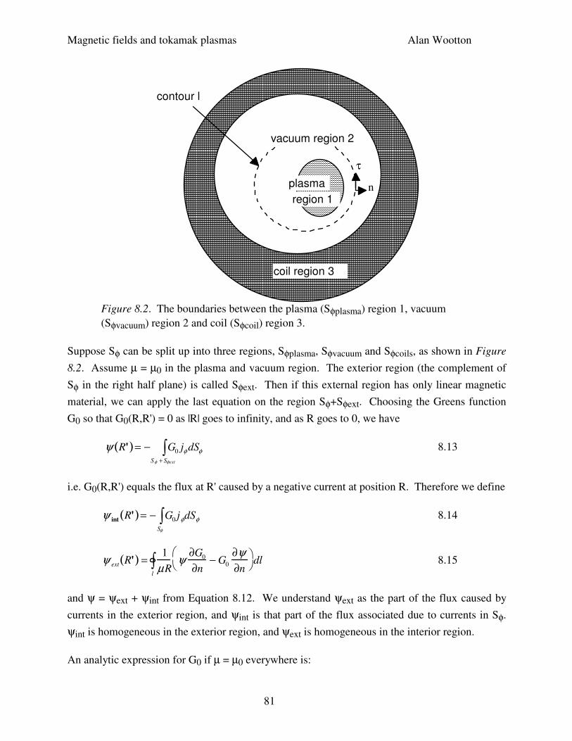
Magnetic fields and tokamak plasmas Alan Wootton
81
plasma
coil region 3
region 1
vacuum region 2
contour l
τ
n
Figure 8.2. The boundaries between the plasma (Sφplasma) region 1, vacuum
(Sφvacuum) region 2 and coil (Sφcoil) region 3.
Suppose Sφ can be split up into three regions, Sφplasma, Sφvacuum and Sφcoils, as shown in Figure
8.2. Assume µ = µ0 in the plasma and vacuum region. The exterior region (the complement of
Sφ in the right half plane) is called Sφext. Then if this external region has only linear magnetic
material, we can apply the last equation on the region Sφ+Sφext. Choosing the Greens function
G0 so that G0(R,R') = 0 as |R| goes to infinity, and as R goes to 0, we have
ψ R'( )= − G0 jφ dSφSφ + Sφext
∫ 8.13
i.e. G0(R,R') equals the flux at R' caused by a negative current at position R. Therefore we define
ψ int R'( )= − G0 jφdSφSφ
∫ 8.14
ψ ext R'( ) =1
µRl
∫ ψ∂G0
∂n− G0
∂ψ∂n
dl 8.15
and ψ = ψext + ψint from Equation 8.12. We understand ψext as the part of the flux caused by
currents in the exterior region, and ψint is that part of the flux associated due to currents in Sφ.
ψint is homogeneous in the exterior region, and ψext is homogeneous in the interior region.
An analytic expression for G0 if µ = µ0 everywhere is:
Magnetic fields and tokamak plasmas Alan Wootton
82
G0 R, R'( ) =µ0
kπRR' E k
2( )− 1 −k2
2
K k
2( )
8.16
where
k2 =
4RR'
R + R'( )2 + z − z'( )2( ) 8.17
Ideal MHD
Here we want to note only one important equation, which is a generalization of the “virial”
equation. We use Equations 6.1, 1.1 and 1.2. Allow the total equilibrium field to be split up into
two parts,
B = B1 + B2 8.18
with ∇xB2 = 0. We can choose the partitioning of B in a number of ways. Multiplying jxB =∇p
by an arbitrary vector Q, we can obtain
p + B1
2
2µ 0
∇• Q − B1 • ∇Q • B1
µ0
V
∫ dV
= p + B1
2
2µ0
Q • n( ) −
B1 • Q( )• B1 • n( )µ 0
Sn
∫ dSn − Q • j × B2( )dVV
∫
8.19
with n the normal to the surface Sn. We have made use of the vector identity
Q ∇ × B • B[ ]= ∇ • Q • B( )B −B2
2Q
+
B2
2∇ • Q − B B • ∇( )Q
We shall use equation 8.19 later to derive important integral relationships.
Boundary conditions
Last in this section we turn to boundary conditions. Suppose we have our three regions, as in
Figure 8.2. Region 1 (Sφplasma) contains all the plasma current. Region 2 (Sφvacuum) contains no
source, but contains a contour l on which we make measurements. Region 3 (Sφcoils) is outside
region 2, extends to infinity, and contains all external currents. To find the plasma boundary we
have to know ψ(R,z) in region 2 between the contour on which parameters are measured, and the
plasma boundary itself. In principle we can do this knowing either
Magnetic fields and tokamak plasmas Alan Wootton
83
a) ∂ψ/∂n (i.e. the tangential field) and either ∂ψ/∂τ (the normal field) or ψ on part of l (note
specifying ∂ψ/∂τ is equivalent to specifying ψ to within an unimportant constant after integration.
This is the Cauchy condition. However, there are significant problems with stability to small
errors in the measurements. Therefore another useful set of boundary conditions is
b) all currents in region 3, and either ∂ψ/∂n, ∂ψ/∂τ or ψ on l. For example, suppose we know the
currents and ψ on l. The total fields are then the superposition of the contributions from the
external currents in region 3 and the plasma current in region 1:
ψ R, z( ) = ψ plasma + ψexternal 8.20
ψexternal is already specified by specifying the external currents, so we must only determine
ψplasma. Since ψplasma is homogeneous outside l, it must be completely specified by the
condition ∂ψplasma/∂n = 0 at infinity and either ψplasma (Dirichlet) or ∂ψplasma/∂n on l
(Neumann). But condition 2 tells us we already have one of these specified, so that ψplasma must
be determined everywhere outside and on l.
In fact we usually use an apparently over determined problem, for example knowing the external
currents, ∂ψ/∂n and ∂ψ/∂τ on l. In fact this is not over determined because we only have the
fields at discrete points, and usually the boundary conditions are only applied in a least squares
sense.
Magnetic fields and tokamak plasmas Alan Wootton
84
9. MOMENTS OF THE TOROIDAL CURRENT DENSITY
Let Θ be an arbitrary function satisfying the homogeneous equilibrium equation L*Θ = 0 in Sφ,
and let ψ be the poloidal flux function which satisfies L*ψ = -µRjφ. Apply Green's second
identity for the operator L* (Equation 8.11) to the pair (Θ,ψ):we obtain a fundamental integral
equation:
ΘΘΘΘjφ dSφSφ
∫ =1
µRψ
∂ΘΘΘΘ∂n
− ΘΘΘΘ∂ψ∂n
l
∫ dl 9.1
The moments of the current density (i.e. the integral on the LHS) are expressed in terms of ψ and
∂ψ/∂n on the boundary. From L*Θ = 0 we have ∫lR-1µ-1(∂Θ/∂n)dl = 0 so there is no dependence
upon the choice of the arbitrary constant in ψ. We introduce together with Θ a conjugate function
ξ according to the equation
∇ξ
µR
=
∇ΘΘΘΘ × ∇φµ
9.2
which admits a solution L*Θ = 0. In cylindrical geometry, Equation 9.2 is
∂
∂R
ξµR
= −
1
µR
∂ΘΘΘΘ∂z
9.3
∂
∂z
ξµR
= −
1
µR
∂ΘΘΘΘ∂R
9.4
The function ξ satisfies L(R-1µ-1ξ) = 0, (remember the operator L = µ−1∇.(µ∇ψ), which reduces
to the Laplacian if µ is uniform). Therefore the definition of ξ implies through Equations 9.3 and
9.4 that −∂(R-1µ-1ξ)/∂τ = R-1µ-1∂Θ/∂n, where ∂/∂τ is the partial derivative along l (clockwise on
the outer boundary). Now by partial integration we can eliminate ψ from Equation 9.1 and write
in terms of ∂ψ/∂τ:
ΘΘΘΘjφ dSφSφ
∫ =1
µRξ
∂ψ∂τ
− ΘΘΘΘ∂ψ∂n
l
∫ dl =1
µξBn + ΘΘΘΘBτ( )
l
∫ dl 9.5
i.e. the "moments" over the current density can be measured as line integrals of the normal (Bn =
(1/R)∂ψ/∂τ) and tangential fields (Bτ = -(1/R)∂ψ/∂n) along the contour l.
Magnetic fields and tokamak plasmas Alan Wootton
85
An alternate derivation follows by letting fields q and g satisfy the equation 1
µ∇ × q( ) = ∇
g
µ
,
so that ∇ × ∇ × q( ) = 0 . Then
q • jdVV
∫ = q. ∇ × B
µ
V
∫ dV = ∇• B
µ× q
+ B
µ• ∇ × q( )
V
∫ dV
= ∇ •B
µ× q
+ B• ∇
g
µ
V
∫ dV =B
µ× q
• n +
g
µ
B • n
Sn
∫ dSn
9.6
This has not invoked axisymmetry. Letting q = Θ∇φ = and g = R-1ξ , and using Equations 8.1
and 8.2 gives the previous result (Equation 9.5).
To get the notation used by Shafranov, we let q = f∇φ (which has a component only in the f
direction, q = f/R) and consider uniform permeability µ0. Then we can write an expression for
the "multipole moment" Ym of the toroidal current density
Ym =1
Ip
fm jφ dSφSφ
∫ =1
µ0 Ip
fm Bτ + Rgm Bn( )l
∫ dl 9.7
where, from Equations 9.3 and 9.4, (i.e. 1
µ∇ × q( ) =
1
µ∇ ×
f
Reφ
= ∇
g
µ
) fm and gm are
various solutions of
∂g
∂R= −
1
R
∂f
∂z 9.8
∂g
∂z=
1
R
∂f
∂R 9.9
Remember that ∇x(∇xq) = 0, with q = f∇φ = eφf/R, so the equation for f is
∂2 f
∂R2 −
1
R
∂f
∂R+
∂2 f
∂z2 = 0 9.10
That is, f is a solution of the homogeneous equilibrium equation and g is a solution of Laplace's
equation. Of course, the trick is to find useful expressions for fm (equivalent to Θm) and gm.
An important point about the method of multipole moments is that the results obtained are
sensitive only to currents flowing within the contour l (including vacuum vessel currents if the
measurements are made outside this). Thus either the total equilibrium fields, or just the plasma
Magnetic fields and tokamak plasmas Alan Wootton
86
fields, can be used. The plasma fields can be calculated if external conductor currents are known.
Using just the plasma fields alone may have advantages in terms of requiring fewer moments to
accurately describe the data.
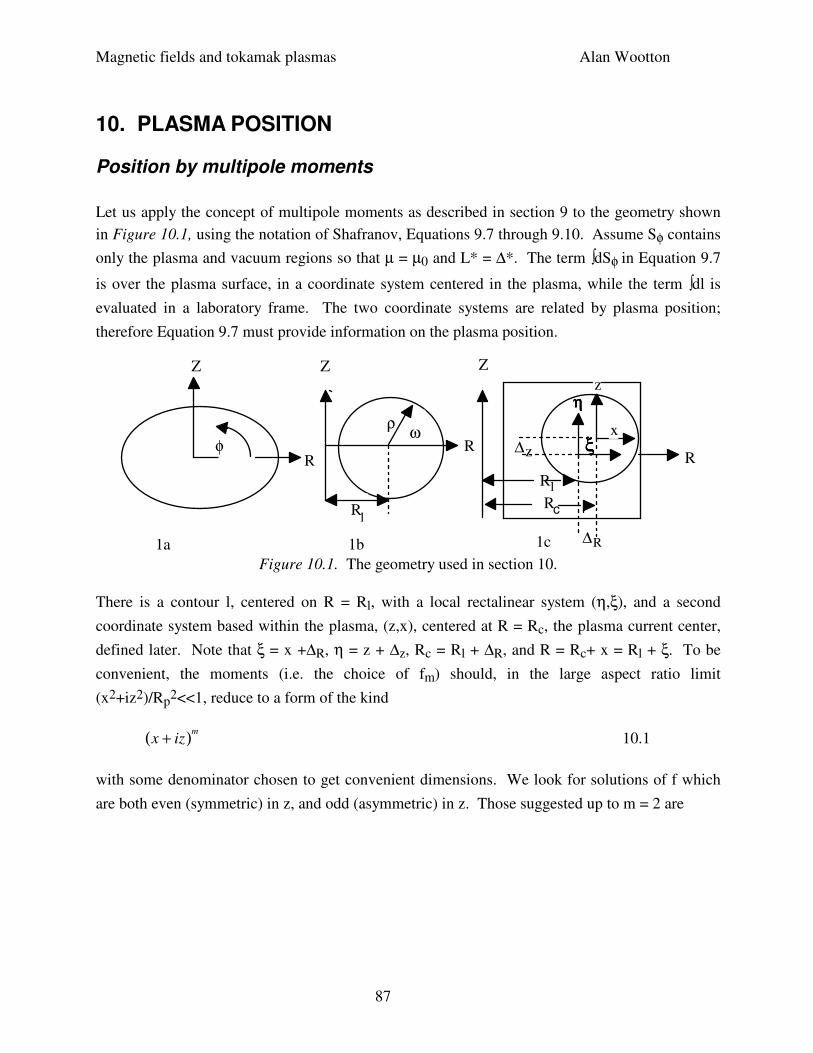
Magnetic fields and tokamak plasmas Alan Wootton
87
10. PLASMA POSITION
Position by multipole moments
Let us apply the concept of multipole moments as described in section 9 to the geometry shown
in Figure 10.1, using the notation of Shafranov, Equations 9.7 through 9.10. Assume Sφ contains
only the plasma and vacuum regions so that µ = µ0 and L* = ∆*. The term ∫dSφ in Equation 9.7
is over the plasma surface, in a coordinate system centered in the plasma, while the term ∫dl is
evaluated in a laboratory frame. The two coordinate systems are related by plasma position;
therefore Equation 9.7 must provide information on the plasma position.
Z
Rω
ρ
1b
Z
R
1c
ηηηη
Rl
Z
1a
ξξξξR
φ
Rl
Rc
∆R
z∆
z
x
Figure 10.1. The geometry used in section 10.
There is a contour l, centered on R = Rl, with a local rectalinear system (η,ξ), and a second
coordinate system based within the plasma, (z,x), centered at R = Rc, the plasma current center,
defined later. Note that ξ = x +∆R, η = z + ∆z, Rc = Rl + ∆R, and R = Rc+ x = Rl + ξ. To be
convenient, the moments (i.e. the choice of fm) should, in the large aspect ratio limit
(x2+iz2)/Rp2<<1, reduce to a form of the kind
x + iz( )m 10.1
with some denominator chosen to get convenient dimensions. We look for solutions of f which
are both even (symmetric) in z, and odd (asymmetric) in z. Those suggested up to m = 2 are
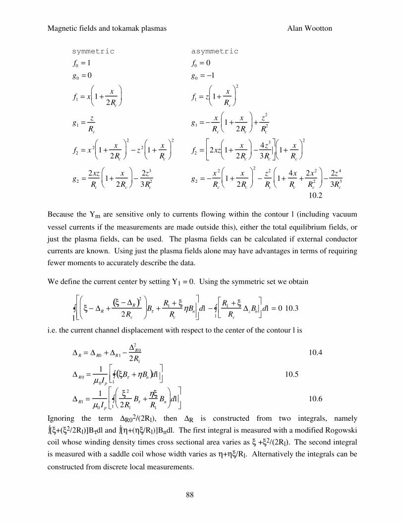
Magnetic fields and tokamak plasmas Alan Wootton
88
symmetric asymmetric
f0 = 1 f0 = 0
g0 = 0 g0 = −1
f1 = x 1 +x
2Rc
f1 = z 1+
x
Rc
2
g1 = z
Rc
g1 = − x
Rc
1 + x
2Rc
+
z2
Rc
2
f2 = x 2 1 +x
2Rc
2
− z 2 1 +x
Rc
2
f2 = 2xz 1+x
2Rc
−
4z3
3Rc
1+
x
Rc
2
g2 =2xz
Rc
1+x
2Rc
−
2z3
3Rc
2 g2 = −x 2
Rc
1 +x
2Rc
2
−z2
Rc
1+4x
Rc
+2x2
Rc
2
−
2z 4
3Rc
3
10.2
Because the Ym are sensitive only to currents flowing within the contour l (including vacuum
vessel currents if the measurements are made outside this), either the total equilibrium fields, or
just the plasma fields, can be used. The plasma fields can be calculated if external conductor
currents are known. Using just the plasma fields alone may have advantages in terms of requiring
fewer moments to accurately describe the data.
We define the current center by setting Y1 = 0. Using the symmetric set we obtain
ξ − ∆R +ξ − ∆R( )2
2Rc
Bτ +
Rl + ξRc
ηBn
dl
l
∫ −Rl + ξ
Rc
∆z Bn
dl
l
∫ = 0 10.3
i.e. the current channel displacement with respect to the center of the contour l is
∆ R = ∆ R0 + ∆R1 −∆ R0
2
2Rl
10.4
∆ R0 =1
µ 0Ip
ξBτ +ηBn( )l
∫ dl
10.5
∆ R1 =1
µ0 I p
ξ 2
2Rl
Bτ +ηξRl
Bn
l
∫ dl
10.6
Ignoring the term ∆R02/(2Rl), then ∆R is constructed from two integrals, namely
∫[ξ+(ξ2/2Rl)]Bτdl and ∫[η+(ηξ/Rl)]Bndl. The first integral is measured with a modified Rogowski
coil whose winding density times cross sectional area varies as ξ +ξ2/(2Rl). The second integral
is measured with a saddle coil whose width varies as η+ηξ/Rl. Alternatively the integrals can be
constructed from discrete local measurements.
Magnetic fields and tokamak plasmas Alan Wootton
89
Consider as an example a circular contour of radius al based on R = Rl. Then ξ = al cos(ω) and η
= al sin(ω). These coils measure the fields in the coordinate system (ρ,ω,φ) based on the vessel
center, and Bn = Bρ , Bτ = Bω. Assuming a plasma with no vertical displacement, symmetric
about z = 0, we can write
Bω = Bτ =µ0I
2πal
1 + λ n cos nω( )n
∑
10.7
Bρ = Bn =µ 0 I
2πal
µn sin(nω )n
∑
10.8
Substituting these expressions into Equations 10.4 to 10.6 gives
∆ R ≈al
2λ1 + µ1( )+
al
2
4Rl
1 +λ2
2+ µ2
−
al
2
8Rl
λ1 + µ1( )2 10.9
i.e. for small displacements, (λ1+µ1) << 1, and a circular plasma (λn, µn, = 0 for n >1) we have,
∆∆∆∆ R ≈al
2λ1 + µ1( )+
al
2
4Rl
10.10
i.e. all that is needed to measure the displacement of a nearly circular plasma within a circular
contour (λn, µn, n ≥ 2 = 0) is a modified Rogowski coil whose winding density varies as cos(ω),
and a saddle coil whose width varies as sin(ω). This simple coil set gives the correct answer
when the constant al2/(4Rl) is allowed for. We already knew this. To allow for significant non-
circularity the more general expression (Equations 10.4, 10.5 and 10.6) should be used. We can
also derive equations to determine the vertical displacement of an arbitrarily shaped plasma,
using the asymmetric components in Equation 10.2.
Application to the large aspect ratio circular tokamak
Let us apply these ideas to the circular equilibrium described in section 6, surrounded by a
circular contour on which we have a sinusoidal area Rogowski coil and a cosinusoidal width
saddle coil. The equations given in section 6 were in a coordinate system (r,θ,φ) based on the
plasma geometric center; they were transformed into the vacuum vessel coordinate system in
section 7, Equations 7.1, 7.2 and 7.3, allowing for a geometric shift ∆g.
The output from the integrated saddle coil with nw layers of width w(ω) = w0sin(ω) and integrator
time constant τint is
Magnetic fields and tokamak plasmas Alan Wootton
90
εµ 1 =nww0al
τ int
Bρ ω( )sin ω( )0
2π
∫ dω =nw w0µ0 I p
τ int 2µ1 10.11
Using the expression for Bρ from Equation 7.3 we get
µ1 =∆∆∆∆ g
al
−al
2Rl
lnal
a p
+ ΛΛΛΛ +
1
2
1−
ap
2
al
2
10.12
The output from the integrated 'modified Rogowski coil each turn of area A, with n0cos(ω) turns
per unit length, is.
ελ 1 =n0 Aal
τ int
Bω ω( )cos ω( )0
2 π
∫ dω =n0 Aµ 0I p
τ int 2λ1 10.13
Using the expression for Bω from Equation 7.2 we obtain
λ1 = −∆∆∆∆g
al
−al
2Rl
lnal
ap
+ ΛΛΛΛ +
1
2
1 +
ap
2
al
2
−1
= −a
l
Rl
ΛΛΛΛ + lna
l
ap
− µ1
10.14
Before we can substitute these expressions (Equations 10.13 and 10.14) into Equation 10.10, we
must recognize that our equilibrium fields were evaluated in a left handed coordinate system,
while this section we have worked in a right handed system. Sorting this out we find λ1 ⇒ -λ1,
and µ1 ⇒ µ1, so that
∆∆∆∆ R − ∆∆∆∆g =ap
2
2Rl
ΛΛΛΛ +1
2
10.15
This is the difference between the geometric center ∆g and the current center ∆R of a circular
plasma, under the present approximations. We also note that, after sorting out the coordinates,
subtracting the outputs from our coils gives
λ1 − µ1 =al
Rl
ΛΛΛΛ + lnal
ap
10.16
that is, we can measure
Magnetic fields and tokamak plasmas Alan Wootton
91
βI +li
2= ΛΛΛΛ +1 = 1+
Rl
al
λ1 − µ1( )− lnal
ap
10.17
Combining Equations 10.15 and 10.16, we see that we can measure the current center, the
geometric center, and Λ, using our modified Rogowski and saddle coils.
Magnetic fields and tokamak plasmas Alan Wootton
92
11. PLASMA SHAPE
Using higher order moments we can obtain information on the plasma shape. Y2 determines
ellipticity and Y3 determines triangularity. Using equations 9.7 and 10.2, we obtain:
Y2 = 1 −2∆R
Rl
s3
τ + s4
n( )s0
τ + ∆z
2 − 1 −∆ R
Rl
∆ R
2 11.1
where
s3
τ = ξ21 +
ξRl
−η2
1+2ξRl
Bτ dl
l
∫ 11.2
s4
n = 2ξη 1 +3ξ
2Rl
−η2
3Rl ξ
Bndl
l
∫ 11.3
s0
τ = Bτdll
∫ = µ0Ip 11.4
That is, with the Rogowski coil measuring Ip (i.e. s0τ) and either modified Rogowski and saddle
coils, or single point measurements of Bn and Bτ suitably combined, we can construct Y2. If we
want to use modified Rogowski and saddle coils, then to obtain Ip, ∆R and Y2 takes a total of 5
coils. For a circular contour, and ignoring toroidal effects, Equation 11.1 is written as
Y2 = −∆ R
2 + ∆z
2 +al
2
2λ2 + µ2( ) 11.5
That is, neglecting toroidal effects we need only λ2 and µ2, in addition to ∆R and Ip.
To interpret the moments it is necessary to assume a plasma current distribution; because the
moment is an integral of the current density over the surface Sφ there is no unique solution for the
boundary shape. As an example, consider a uniform current density and a surface described by an
ellipse with minor and major half width and half height a and b, so that x
a
2
+z
b
2
=1 . Then
for k =b
a−1, k << 1, and ignoring toroidal effects, we have
Y2 ≈ −ka2
2 11.6
In a similar manner, if the surface is described by a function which includes both elongation and
triangularity, namely
Magnetic fields and tokamak plasmas Alan Wootton
93
x
a
2
+z
b
2
+2γx
a
x
a
2
−3z
b
2
=1 11.7
then ignoring toroidicity (i.e. x/Rl and z/Rl <<1, we have for a flat current distribution
Y3 ≈ −a3γ 11.8
Magnetic fields and tokamak plasmas Alan Wootton
94
12. MOMENTS OF PLASMA PRESSURE
The Virial Equation
Here we consider certain integral relations which allow us to determine information on the energy
density within Sφ. The techniques described to determine plasma position, and more generally
plasma shape, needed only Maxwell's equations. Now we add the constraint of equilibrium.
Generally we apply these results to Sφ = Sφplasma + Sφvacuum: even simpler relations are obtained
by identifying Sφ with Sφplasma.
From a previously derived integral equation (Equation 8.19), we can obtain some very useful
relationships. First, take B2 = 0 (i.e. all the fields are described by B = B1), and let the arbitrary
vector Q be the polar vector (r = ReR + zeZ.). Then Equation 8.19 becomes the “virial theorem”:
3p +B2
2µ 0
V
∫ dV = p +B2
2µ 0
r • n( ) −
r • B( ) B •n( )µ 0
Sn
∫ dSn 12.1
Note that if B were the self plasma field, and there was no other field, then the surface integral on
the RHS approaches zero as the surface (where p = 0) approaches infinity, because B(self) ∝ R-3.
This contradicts the positive definiteness of the LHS volume integral, showing that equilibrium
by self fields alone is impossible.
Now restricting to toroidal symmetry, ∂/∂φ = 0. Therefore the poloidal (subscript p) and toroidal
(subscript φ) fields satisfy
B = Bp + Bφ
Bp •Bφ = 0 12.2
Next assume that the surface Sn is outside the plasma, where ∇xB = 0, and that the vectors Q and
B2 are purely poloidal (i.e. there is no toroidal component of B2);
Q = QReR + Qz ez
B2 = B2ReR + B2 zez
12.3
Noting that the toroidal field outside the plasma is given by Bφe = const/R, then we have
Bφe
2
Sn
∫ Q • n( )dSn = Bφe
2
V
∫ ∇ • Q −2Q • eR
R
dV 12.4
Magnetic fields and tokamak plasmas Alan Wootton
95
and
B1 • B1 • ∇Q = Bp1 •Bp1 •∇Q +Bφe
2Q • eR
R 12.5
Using these, we can express Equation 8.19 so that the toroidal field enters only as Bφ2-Bφe2 on
the LHS:
p +Bp1
2
2µ 0
∇• Q +
Bφ2 − Bφe
2
2µ0
∇ • Q − 2Q •eR
R
−
Bp1 •∇Q • Bp1
µ 0
V
∫ dV
= p +Bp1
2
2µ0
Q • n( ) −
Bp1 • Q( )Bp1 •n( )µ0
Sn
∫ dSn − j • Bp2 × Q( )[ ]V
∫ dV
12.6
Now let
P = p +Bφ
2 − Bφe
2
2µ 0
12.7
T = p +Bp1
2 + Bφe
2 − Bφ2
2µ 0
12.8
(Remember B1 is the poloidal field). Then the integrand on the LHS of Equation 12.6 can be
written as (from now on drop the subscript p for poloidal)
. ..[ ]= P∂QR
∂R+
∂Qz
∂z
+T
RQR +
B1R
2 − B1z
2
2µ 0
∂Qz
∂z−
∂QR
∂R
−B1R B1z
µ 0
∂QR
∂z+
∂Qz
∂R
12.9
Now we have to chose something for Q. Let
u = R − Rch + iz = ρeiω
12.10
with Rch some characteristic radius, a fixed point within the plasma cross section. Then
ρ2 = R − Rch( )2
+ z2
12.11
Now with this notation let
QR = F u( )Qz = −iF u( )
12.12
Magnetic fields and tokamak plasmas Alan Wootton
96
so that the last two terms in Equation 12.9 are zero. Next take
F u( ) = um +1
12.13
Finally we can rewrite Equation 12.6 in the form
2 m +1( )Pum +
T
Ru
m+1
V
∫ dV
= p +B1
2
2µ0
n R − inz( )−
B1R
− B1z( ) B
1•n( )
µ 0
Sn
∫ um+1dSn − j • B2 × Q( )[ ]V
∫ dV
12.14
Surprisingly, this is useful. We now consider the results when we take different values of m.
m = -1, B2 = Bext
Take B2 as the externally supplied maintaining field and B1 the plasma self field. For large
volumes the surface integral approached zero, and we have
−T
RV
∫ dV = jφ Bz, extdVV
∫ 12.15
or equivalently
jφ Bz ,ext RdSφSφ
∫ = − p +Bp1
2 + Bφe
2 − Bφ2
2µ0
dSφ
Sφ
∫ 12.16
Suppose (low toroidicity) that ρ/Rch <<1. Then the R dependence of T appears in the form R -
Rch, so that dT/dR = -dT/dRch. Now because T/R = ∇.TeR - dT/dR (if ρ/Rch <<1) we have, with
T = 0 at infinity:
T
RV
∫ dV = −∂T
∂RV
∫ dV ≈∂
∂Rch
TdV∫( ) 12.17
Now introduce some definitions:
B⊥ = −1
2πRch I p
jφ Bz,extdVV
∫ 12.18
Magnetic fields and tokamak plasmas Alan Wootton
97
RT =
TRdSφSφ
∫
TdSφSφ
∫ 12.19
Lpt =8π
µ0 Ip
2
Bp1
2
2µ 0V
∫ dV 12.20
βI =8π
µ0Ip
2 pdSφSφ
∫ 12.21
µ I = −8π
µ0Ip
2
Bφ2 − Bφe
2
2µ0
dSφ
Sφ
∫ 12.22
Note that µ0Lpt/(4π) is a total inductance, and the usual "inductance per unit length times 4π/µ0"
is given as
Lp =4
µ 0Rch Ip
2
Bp
2
2µ 0V
∫ dV 12.23
Now we can write Equation 12.16 as
B⊥ =µ0 I p
8πRch
β I + µ I +∂
∂Rch
Rch Lp( )
12.24
This is a generalization of the external vertical field needed to maintain a plasma, allowing for
non circularity.
m = 0, B2 = 0
Now Equation 12.14 gives an integral expression along the minor radius:
PdV +RT − Rch( )
2RTV
∫ TdVV
∫
= 0.5Bτ1
2 − Bn12( )
2µ0
n •eρ − Bτ 1Bn1
µ0
τ •eρ
Sn
∫ ρdSn − 0.5 jφV
∫ Bz2 R − Rch( )− BR2z[ ]dV
12.25
Magnetic fields and tokamak plasmas Alan Wootton
98
If we assume that |R-Rch| << Rch, then the term with (RT-Rch)/(2RT) can be omitted, and the LHS
is independent of the choice of Sn. Therefore the RHS must also be independent of Sn. Then we
can write (with |R-Rch| << Rch)
PdVV
∫ =µ 0 Rch Ip
2
4s1 12.26
where s1 must be independent of the choice of B2. In particular, taking B2 = 0, Equation 12.25
can be written, using the definitions above, as
βI = µ I + s1 12.27
where
s1 =1
µ0
2RchIp
2 Bτ2 − Bn
2( )ρn • eρ − 2Bτ Bnρττττ •eρ[ ]dSn
Sn
∫ 12.28
The difference between s1 and 1 is due to non circularity.
In fact, the constraint R-Rch| << Rch, but not (RT-Rch)/(2RT), can be relaxed by redefining βIv
and µIv as volume integrals: see Equations 12.31 and 12.32 below.
m = -1, B2 = 0
Now we obtain another important integral relationship, assuming |R-Rch| << Rch, namely
βI +Lp
2=
s1
2+ s2 12.29
where
s2 =1
µ 0
2I p
2 Bτ2 − Bn
2( )n • eς − 2Bτ Bnττττ • eς[ ]dSn
Sn
∫ 12.30
and ζ = R - Rch.
In fact, the approximation |R-Rch| << Rch is not necessary if β and µ are redefined as volume
integrals, namely
2πRchβIV =8π
µ 0 Ip
2 pdVV
∫ 12.31
Magnetic fields and tokamak plasmas Alan Wootton
99
2πRchµ IV = −8π
µ 0 I p
2
Bφ2 − Bφe
2( )2µ 0
dVV
∫ 12.32
Magnetic fields and tokamak plasmas Alan Wootton
100
13. ββββI + li/2
Solution
In the previous section, Equation 12.29, we showed that we could express the parameter βI + Lp/2
through the integral equation
βI +Lp
2=
s1
2+ s2 13.1
where s1 and s2 are two integrals of the fields over dSn, which we will be able to measure as
contour integrals, namely
s1
= 1
µ0
2RchIp
2Bτ
2 − Bn
2( )ρn • eρ − 2Bτ Bnρττττ •eρ[ ]dSn
Sn
∫
=2π
µ 0
2RchI p
2Bτ
2 − Bn
2( )ρn • eρ − 2BτBnρττττ •eρ[ ]Rdll
∫ 13.2
s2
= 1
µ 0
2I p
2Bτ
2 − Bn
2( )n • eς − 2Bτ Bnττττ • eς[ ]dSn
Sn
∫
=2π
µ 0
2I p
2Bτ
2 − Bn
2( )n • eς − 2Bτ Bnττττ • eς[ ]Rdll
∫ 13.3
Equation 13.1 was good for toroidal geometry if volume definitions βIV and µIV were used. Note
that dSn = 2πRdl, so that s1 and s2 can be written as contour integrals around l. Unfortunately
they involve the squares of fields, and so we cannot design simple modified Rogowski and saddle
coils to make the measurements. Instead we must measure Bn and Bτ at discrete points along the
contour, and then construct the required integrals. All we have to do is construct the integrals s1
and s2 from measured Bn and Bτ.
Suppose we are measuring fields on a circular contour of radius al, centered at R = Rl = Rch; that
is we identify our characteristic radius with the center of the contour l. Then in the vessel
coordinates we have ττττ.eρ = 0, n.eρ = 1, n.eζ = cos(ω), ττττ.eζ = -sin(ω), and dSn =
2πRl[1+(al/Rl)cos(ω)]aldω. If the fields can be expanded as in Equations 10.7 and 10.8, and
keeping only the terms λ1 and µ1 (i.e. a circular plasma), we obtain
Magnetic fields and tokamak plasmas Alan Wootton
101
s1 = 1
s2 = Rl
al
λ1 + µ1( ) 13.4
i.e., substituting 13.4 into 13.1:
βI +Lp
2= 1+
Rl
al
λ1 + µ1( ) 13.5
Let us apply this equation to the displaced analytic equilibrium discussed in sections 6 and 9.
The Rogowski coil with cosinusoidal varying winding density, and the saddle coil with sinusoidal
varying width, tell us λ1 and µ1. First there is a mess with right and left handed coordinate
systems to unravel. Doing this then µ ⇒ -µ in Equation 13.5. Now Equation. 10.16 already tells
us that
λ1 − µ1 =al
Rl
lnal
ap
+ β I +
li
2−1
13.6
Therefore comparing Equations 13.5 and 13.6 we must have (allowing µ ⇒ -µ in Equation 13.5)
that
li
2+ ln
al
ap
=
Lp
2 13.7
This is exactly what we expect, because the total inductance to a radius al is given by:
Ltotal = 2πRµ 0
4π
Lp = µ0 R ln
al
ap
+
li
2
13.8
Separation of ββββI and li
If we have βI + li/2 from the poloidal field measurements just described, and βI from diamagnetic
measurements (see later) then obviously we can separate βI and li If no diamagnetic
measurement is available, two possibilities exist. For non circular plasmas, there is a third
integral relationship, which I have not derived, which gives in terms of a measurable line integral
the parameter ∫V
(2p+Bz2/µ0)dV. When V is the plasma volume, this is related to 2βI + Lp. If the
volume averages <Bz2> and <Bp2> are different, as is the case for non circular discharges, then
this measurement allows the separation.
Magnetic fields and tokamak plasmas Alan Wootton
102
For near circular plasmas, we must estimate Lp separately. For example, for the simple circular
low beta equilibrium of section 6, we can take a model current distribution jφ0(r) = j0(1-(r/a)2)α.
Then li = Lp-ln(al/ap), with li given as a function of α = (qa/q0 -1). By assuming q0 = 1 we can
then estimate li, and make the separation.
Comments on the definition of poloidal beta
We must be careful with the definition of "poloidal beta". So far we have used Equation 12.21,
namely
βI =8π
µ0Ip
2 pSφSφ
∫ 13.9
We could replace βI by βp (the poloidal beta), which characterizes the ratio of plasma pressure to
the pressure of the magnetic field for an arbitrary shaped cross section. It should be introduced so
that the pressure balance, Equation 12.27, is replaced by
β p = 1 + µp 13.10
so that βp = 1 for µp = 0.
Magnetic fields and tokamak plasmas Alan Wootton
103
14. DIAMAGNETISM
Comments
Next we turn to the toroidal flux and its measurement. Before plasma initiation this is simply
given by Bφdll
∫ = µ0 jzdSS
∫ , i.e. 2πRBφ = µ0 Iz , where we have applied Amperes law to a contour
in the toroidal direction, encircling the inner vertical legs of the toroidal field coils (i.e. Iz =
izntnc, with iz the current from the generator, nc the number of assumed series coils, and nt the
assumed series number of turns in each coil).
Microscopic picture for a square profile plasma in a cylinder
During formation inside a magnetic field the plasma particles acquire a magnetic moment m:
m = Areaorbit Iorbit = πv
ω
2qω2π
14.1
Since ω = qB/me, we have
m =mev
2
2B 14.2
adding up to a total magnetic moment
M = nmSφ 14.3
per unit length of column with cross section Sφ and a number density of n Supposing cylindrical
geometry the elementary currents cancel within the homogeneous column, leaving only an
azimuthal surface "magnetization' current density js:
js = nm =nkbT
B=
p⊥
B 14.4
where p⊥ = nkb(Te + Ti)⊥, kb is Boltzmann’s constant. The toroidal field will be modified.
The associated flux from this surface current can be calculated:
Magnetic fields and tokamak plasmas Alan Wootton
104
∆Φ∆Φ∆Φ∆Φ = πap
2 ∆∆∆∆Bφ = πap
2 µ 0
2πRI = πa p
2 µ0
2πR2πRjs
= πap
2 µ 0
2πR2πR
p⊥
Bφ
= πap
2µ0
p⊥
Bφ
Using the definition of βI, discussed much more a little later, we then have
∆Φ∆Φ∆Φ∆Φ =µ0
2Ip
2β I
8πBφ
Macroscopic picture
Let us consider a toroidal device with no toroidal current plasma current, i.e. a stellarator, in
which the necessary rotational transform is produced only by external conductors. Starting with
the radial pressure balance, with p⊥= 0 at the plasma edge, and approximating the torus by a long
cylinder, then
dp⊥
dr= jθ Bφ 14.5
integrating over the minor radius (r = 0 to ap) gives
p⊥ = −Bφ jθ r'( )dr'r
ap
∫ 14.6
and
p⊥ = 1
πa p
22π
0
ap
∫ p⊥ rdr = −Bφ
πap
22π
0
ap
∫ rdr jθ r'( )r
ap
∫ dr'
= −Bφ
πap
2π
0
ap
∫ r 2 jθ r( )dr = −Bφ
S r( )πap
2
0
ap
∫ jθ r( )dr
14.7
Then jse = ∫0
apS(r)/(πap
2)jθ(r)dr is the effective surface current density at the plasma edge as a
consequence of the finite plasma pressure.
Magnetic fields and tokamak plasmas Alan Wootton
105
Paramagnetic and diamagnetic flux
Outside the plasma the toroidal field has the form Bφe = Bφ0(R0/R), with Bφ0 the value at a fixed
radius R0. This toroidal field, together with the poloidal field, takes part in balancing the plasma
pressure.
We need an equation relating fields to pressure. Substituting ∇ × B = µ 0 j into ∇p = j × B yields
(using B × ∇ × B( ) =∇B2
2− B • ∇( )B )
∇ p +B2
2µ 0
= B• ∇( ) B
µ0
For a straight axially symmetric system (∂/∂z = 0) we obtain
∂
∂rp +
Bz
2 + Bθ2
2µ0
= −
Bθ2
rµ 0
Multiplying each side by r2, letting u = r2, du = 2rdr, dv = ∂/∂r(.), v = (..), we obtain by
integrating by parts (∫udv = uv - ∫vdu)
r2
p +Bz
2 + Bθ2
2µ0
0
a
− p +Bz
2 + Bθ2
2µ0
0
a
∫ 2rdr = −Bθ
2
µ 00
a
∫ rdr
i.e.,
p +Bz
2 + Bθ2
2µ 0
r = a
=1
πa2 p +
Bz
2
2µ0
0
a
∫ 2πrdr
That is, ignoring curvature and equating Bz with Bφ, the pressure balance constraint is
2µ 0 p = Bθa
2 + Bφe
2 − Bφ2
14.8
where Bφ is the toroidal field inside the plasma, Bφe is the toroidal field outside the plasma, <..>
means an average over the plasma radius, and we have assumed p = 0 at the boundary (i.e. at r =
a). That is, for a given plasma current Ip and pressure <p>, the difference (Bφe2 - <Bφ2>) adjusts
itself to ensure pressure balance. This happens because of a poloidally flowing current, either
diamagnetic or paramagnetic, in the plasma, as we derived in equations 14.4 and 14.17. In a
tokamak we have Bφe2 >> Bφe
2 - <Bφ2>, so that if the cross section is circular with radius ap,
Magnetic fields and tokamak plasmas Alan Wootton
106
Bφe
2 − Bφ2 ≈ 2Bφe Bφe − Bφ =
2BφeδΦΦΦΦ
πa p
2 14.9
where
δΦΦΦΦ = πap
2Bφe − Bφ 14.10
is the diamagnetic flux of the longitudinal (toroidal) field. We will discus its measurement later;
it is the difference in toroidal flux in the plasma column when the plasma is initiated. Defining
βI =8π
µ0Ip
2 pdSφSφ
∫
i.e. βI =2µ0 p
Bθa
2 for a circular cross section 14.11
with Bθa =µ0I p
2πap
the poloidal field at the plasma edge, we can write
βI = 1+8πBφeδΦΦΦΦ
µ 0
2I p
2 14.12
From this equation we write the net flux difference δΦ = (µ0Ip)2/(8πBφe).(βI - 1) as the sum of
the paramagnetic flux δΦp:
δΦΦΦΦp = −µ0
2I p
2
8πBφe
14.13
due to the poloidal component of the force free plasma current, and the diamagnetic flux δΦd:
δΦΦΦΦd = −δΦΦΦΦpβ I 14.14
due to the poloidal currents providing pressure balance for the finite pressure.
Toroidal, non circular geometry
In a torus curvature must be accounted for: Corrections with coefficients (a/R) appear in the RHS
of the equation for βI. For βI << R/a the corrections are small, and it should be noted only that
for Bφe the value on a line R = Rg, the plasma center, should be used. We will derive that below.
Also, we must now be rather careful with definitions.
Magnetic fields and tokamak plasmas Alan Wootton
107
We derived, in section 13, a general expression relating βI to poloidal field measurements and the
diamagnetic measurements. This derivation allowed for both toroidicity and non circularity, and
gave in terms of volume integrals (equations. 12.31, 12.32, 12.27, 12.28)
βIV = µ I + s1 14.15
µ IV = −4
µ 0 Rch I p
2
Bφ2 − Bφe
2( )2µ0V
∫ dV 14.16
βIV =4
µ 0 Rch I p
2 pV
∫ dV 14.17
The measurable integral s1 = 1 for a circular discharge. Remember that Rch was a characteristic
major radius of the plasma. Because we can write |Bφe-Bφ| << Bφ0, the diamagnetic parameter
can be expressed through the experimentally determined flux (the measurement is discussed later)
δΦΦΦΦ = Bφe − Bφ( )dSφSφ
∫ 14.18
By substituting (Bφe2-Bφ2) ≈ 2Bφ(Bφe-Bφ), and writing
Bφe =Bφ 0 Rch
R 14.19
then we have
µ IV =8πBφ 0δΦΦΦΦ
µ0
2Ip
2 14.20
That is, in toroidal geometry and for an arbitrary shaped cross section, measuring δΦ and the
integral s1 gives us a good measure of βIV, the volume defined current beta. Note that the field
Bφ0 is the external field at the characteristic plasma major radius, which we can take as Rch ≈ Rg..
The meaning of ββββI
We can understand βI by integrating by parts Equation 14.11 to give (for a circular cross section),
and assuming p at r = ap = 0, we have
Magnetic fields and tokamak plasmas Alan Wootton
108
βI =8π
µ0Ip
2prdrdθ
0
ap
∫0
2 π
∫ =8π
µ0 I p
22 prdr
0
a p
∫
= 8π 2
µ 0I p
2pr 2
0
a p − r 2 dp
drdr
0
ap
∫
= − 8π 2
µ0 I p
2r 2 dp
drdr
0
ap
∫
14.21
Here we have integrated by parts, with u = p, du = (dp/dr)dr, v = r2, dv = 2rdr. Next we use the
approximate pressure balance equation (dp/dr = jθBφ - jφBθ, we will work in a RH coordinate
system). We substitute for jθ and jφ in terms of Bφ and Bθ (from µ 0 j = ∇ × B), i.e.
µ 0 jθ = −∂Bφ
∂r, µ 0 jφ =
1
r
∂ rBθ( )∂r
, we obtain
dp
dr+
d
dr
Bφ2
2µ0
+
Bθ
µ0r
d
drrBθ( )= 0 14.22
Substituting for dp/dr from equation. 14.22 into equation. 14.21 gives
βI =4π 2
µ0
2 Ip
2
d Bφ2( )
drr 2dr
0
ap
∫ + 2Bθrd rBθ( )
drdr
0
ap
∫
=1
ap
2Bθa
2
d Bφ2( )
drr
2dr
0
ap
∫ + rBθ( )2
0
ap
= 1 +1
ap
2 Bθa
2
d Bφ2( )
drr2 dr
0
ap
∫
14.23
If (dBφ2/dr) > 0 then βI > 1, and if (dBφ2/dr) < 0 then βI < 1. Figure 14.1 shows this
schematically. A reduced Bφ (diamagnetic) inside the plasma is associated with βI > 1. The
normal ohmic heating case, with βI ≈ 0.3 has an increased Bφ inside the plasma (paramagnetic).
The figures are not well drawn, because we must have that BφR is constant on a flux surface.
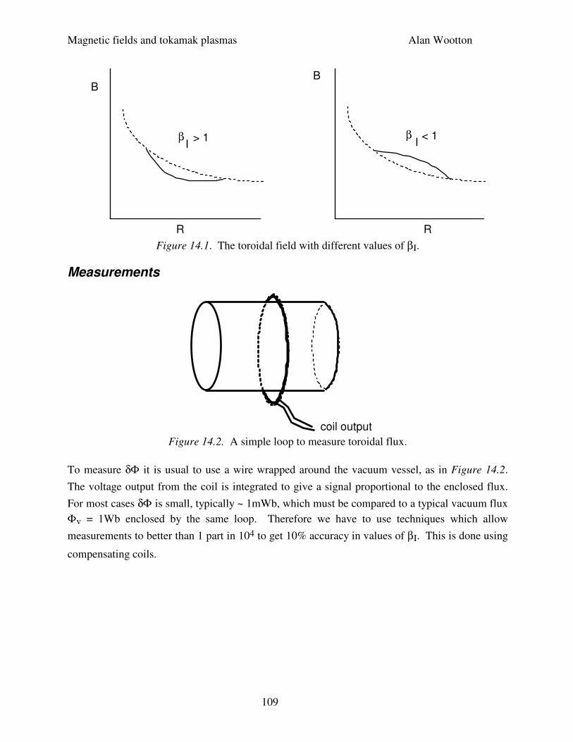
Magnetic fields and tokamak plasmas Alan Wootton
109
B
R
B
R
β I
> 1 βI
< 1
Figure 14.1. The toroidal field with different values of βI.
Measurements
coil output Figure 14.2. A simple loop to measure toroidal flux.
To measure δΦ it is usual to use a wire wrapped around the vacuum vessel, as in Figure 14.2.
The voltage output from the coil is integrated to give a signal proportional to the enclosed flux.
For most cases δΦ is small, typically ~ 1mWb, which must be compared to a typical vacuum flux
Φv = 1Wb enclosed by the same loop. Therefore we have to use techniques which allow
measurements to better than 1 part in 104 to get 10% accuracy in values of βI. This is done using
compensating coils.
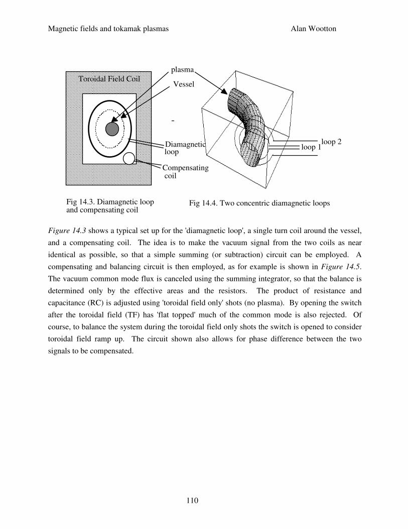
Magnetic fields and tokamak plasmas Alan Wootton
110
Toroidal Field CoilVessel
loop
Compensatingcoil
Fig 14.3. Diamagnetic loop and compensating coil
Fig 14.4. Two concentric diamagnetic loops
loop 1loop 2Diamagnetic
plasma
Figure 14.3 shows a typical set up for the 'diamagnetic loop', a single turn coil around the vessel,
and a compensating coil. The idea is to make the vacuum signal from the two coils as near
identical as possible, so that a simple summing (or subtraction) circuit can be employed. A
compensating and balancing circuit is then employed, as for example is shown in Figure 14.5.
The vacuum common mode flux is canceled using the summing integrator, so that the balance is
determined only by the effective areas and the resistors. The product of resistance and
capacitance (RC) is adjusted using 'toroidal field only' shots (no plasma). By opening the switch
after the toroidal field (TF) has 'flat topped' much of the common mode is also rejected. Of
course, to balance the system during the toroidal field only shots the switch is opened to consider
toroidal field ramp up. The circuit shown also allows for phase difference between the two
signals to be compensated.
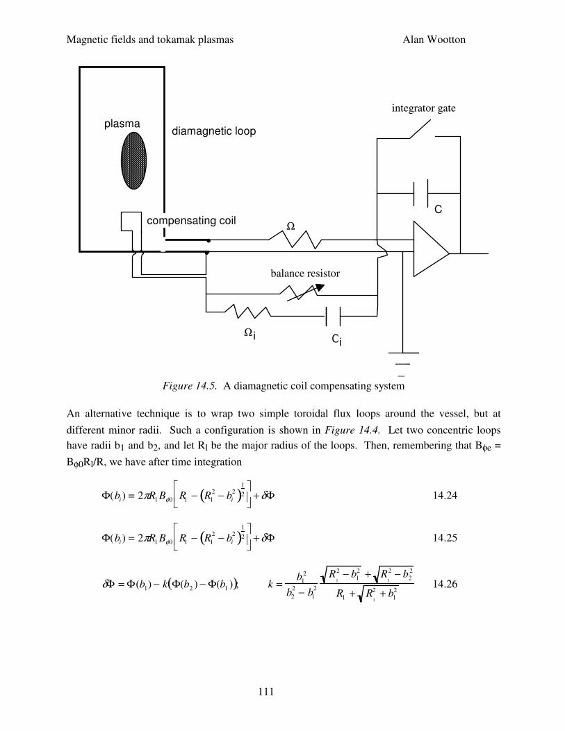
Magnetic fields and tokamak plasmas Alan Wootton
111
diamagnetic loop
compensating coil
_
plasma
Ω
CΩi
i
C
integrator gate
balance resistor
••
Figure 14.5. A diamagnetic coil compensating system
An alternative technique is to wrap two simple toroidal flux loops around the vessel, but at
different minor radii. Such a configuration is shown in Figure 14.4. Let two concentric loops
have radii b1 and b2, and let Rl be the major radius of the loops. Then, remembering that Bφe =
Bφ0Rl/R, we have after time integration
Φ(bi) = 2πRl Bφ0 Rl − Rl
2 − bi
2( )1
2
+δΦ 14.24
Φ(bi) = 2πRl Bφ0 Rl − Rl
2 − bi
2( )1
2
+δΦ 14.25
δΦ = Φ(b1) − k Φ(b2 ) − Φ(b1 )( ); k =b1
2
b2
2 − b1
2
Rl
2 − b12 + R
l
2 − b22
Rl + Rl
2 + b12
14.26
Magnetic fields and tokamak plasmas Alan Wootton
112
From these two signals we can calculate δΦ. The subtractions are performed electronically (i.e.
analog); the constant k is determined experimentally so that δΦ is zero without plasma (toroidal
field only).
In reality there are problems. One in particular is caused by the discreteness of the toroidal field
system, and the current redistribution in the toroidal field coils during a shot. When the toroidal
field current is initiated, the current flows at the inner edge of the conductors to minimize the
linked flux. As the pulse proceeds, the current redistributes and approximates a uniform
distribution (not exactly because of repulsion of current channels). The time for this
redistribution to occur is approximately the radial penetration time of the poloidal current into the
conductor of radial extent w: τ ≈ πµ0σw2/16, typically 200 ms. If the toroidal field system was a
perfect toroidal solenoid this redistribution would leave the fields unaffected. However, because
of the discrete number of toroidal fields, there is now a time varying toroidal field ripple. The
size of the changing field ripple depends on where a pickup coil is placed: therefore two coils
linking the same steady state flux can link different transient fluxes. It is best to place the coils
between the toroidal field coils, where the redistribution effect is smallest.
Another problem is due to poloidal eddy currents in any conducting vacuum vessel. This
produces a non zero change in the toroidally averaged Bφ, not just a local ripple. Therefore it
couples strongly to the pickup loops. Compensation for both the effects discussed has been
performed successfully using software, by simulating redistribution and eddy currents as simple
circuits, coupled to both the primary Bφ coil current and a secondary pickup coil.
Further problems occur if the loops are not exactly positioned, so that they couple to the poloidal
fields produced by the primary, vertical field and shaping windings. That any such effects exist
can be checked for by firing discharges with positive (+) and negative (-) Bφ. Let ∆Φp be the
signal caused by poloidal field coupling, ∆Φ(+) the signal obtained with positive Bφ, and ∆Φ(-)
the signal obtained with negative Bφ. While the toroidal field coupling effects will change sign
with reversing Bφ, any poloidal field effects will not. Therefore
∆Φ∆Φ∆Φ∆Φ +( ) − ∆Φ∆Φ∆Φ∆Φ −( ) = 2 δΦΦΦΦ + ∆Φ∆Φ∆Φ∆Φ p( ) 14.27
∆Φ∆Φ∆Φ∆Φ +( ) + ∆Φ∆Φ∆Φ∆Φ −( ) = 2∆Φ∆Φ∆Φ∆Φ p 14.28
Any finite ∆Φp can be correct for using a circuit model again, with the coupling between any
winding (including vacuum vessel) and the pickup coil written in terms of mutual inductances.
Magnetic fields and tokamak plasmas Alan Wootton
113
15. FULL EQUILIBRIUM RECONSTRUCTION
The problem under discussion is how to reconstruct as much as is possible about the equilibrium
from external measurements. In particular, if we knew everything about the fields outside the
plasma, what could we uniquely determine? Could we separate βI and li? (In principle yes for
toroidal systems). Could we go further and actually uniquely determine the plasma current
distribution of a toroidal plasma (I don't know)?
If we want to allow measurements of dp(ψ)/dψ and FdF(ψ)/dψ we must have redundancy beyond
that required to solve the equilibrium equation with a known current density profile. We see
immediately a problem in straight geometry, because with straight circular cross sections the
magnetic measurements must be consistent with a solution that has concentric circular surfaces.
In this case the measurements are consistent with any profile function which gives the correct
total plasma current, so there is an infinite degeneracy.
In practice the mathematical subtleties of what can and cannot in principle be determined are not
discussed. Instead the usual technique for equilibrium reconstruction is to choose a
parameterization for jφ, with a restricted number of free parameters. These free parameters are
chosen to minimize the chi squared error or cost function between some measured and computed
parameter, for example the poloidal field component on some contour. Obviously we need some
boundary conditions, as discussed in section 8. Information available might consist of the flux ψ
on a contour, the fields Bn and Bτ on a contour, and currents in conductors, the total current, and
if lucky the diamagnetism. Typical parameterizations are
jφ = aβR
R0
+ 1− β( ) R0
R
g δψ( ) 15.1
jφ = α1δψ + α2δψ 2 +α 3δψ 3( )R + b1δψ( )R−1
15.2
with δψ = (ψ-ψboundary)(ψmag axis-ψboundary). In each case the term proportional to R represent
the part of jφ proportional to dp/dψ, and the part of jφ proportional to R-1 is proportional to
FdF/dψ. Ro is some characteristic radius. The assumed function g might be of the form g(δψ,γ)
= exp(-γ2(1-δψ)2, dψγ or δψ + γδψ2. If in equation 15.1 the function g(δψ) is 1, then the
description of jφ is called quasi uniform: for a circular outer boundary there is an exact analytic
solution of the equilibrium equation.
Magnetic fields and tokamak plasmas Alan Wootton
114
The general results show that, given only poloidal field magnetic measurements (i.e. no
diamagnetic signal), then βI and li can only be separated for significantly non circular equilibria.
From our discussions of βI+li/2, we know we can measure βI+Li/2 exactly anyway. If we have
reconstructed the plasma surface then we can evaluate the integrals s1 and s2 on that plasma
surface, and then Li = li. For circular equilibria it is found that only the sum βI + li/2 can be
found. Of course, adding a diamagnetic measurement allows the separation for any shape, as we
have seen. Also adding a pressure profile form, or the pressure on axis, is enough to allow
separation even for circular discharges. It is generally found that a distortion of the shape to b/a ~
1.3 is needed to make the separation.
A significant problem is that, having made specific assumptions about the form of the current
density profile, we do not know how general our results are.
Magnetic fields and tokamak plasmas Alan Wootton
115
16. FAST SURFACE RECONSTRUCTION
Here we want to investigate 'fast' methods of determining the plasma boundary, and fields on that
boundary. If we can do this, then we can exactly derive parameters such as βI + li/2, and q, on the
boundary, as well as parameterizing the boundary shape itself. Here we specifically do not want
to obtain any information on fields and fluxes inside the plasma boundary.
In the vacuum region Sφvacuum bounded by the contour lplasma and l, the flux function satisfies
the homogeneous equation L*ψ = 0. A solution for this equation which agrees with boundary
conditions on l, and that is valid in a region containing Sφvacuum, must then be valid on the
plasma boundary itself.
In general we choose to approximate ψ by a series solution
ψ ≈ ψest = ψ 0 + c jχ j
j =1
N
∑ 16.1
With ψ0 any known terms, and the basis functions all satisfy the homogeneous equilibrium
equation on some region Sφ0 which includes the vacuum region Sφvacuum. Following the
discussion in section 8 we can write ψ = ψext + ψint from Equations 8.12 through 8.15. Usually
we take an interior solution ψint associated with current distributions inside Sφ, and an exterior
part ψext associated with currents in the exterior region Sφext. For example ψext may be known
from measured currents in external conductors, or calculated directly from the measurements
using Green's functions. Various representations for the plasma current have been used;
an expansion in toroidal eigenfunctions,
discrete current filaments,
single layer potential on a control surface,
To date no purely analytic answers are available; generally the coefficients in an expansion, of
position or currents in filaments, are altered numerically to provide a minimum "chi squared"
between some measured and computed fields or fluxes. For example, suppose the actual
measurements are represented by qi, with i running from 1 to M. There is a response matrix Q
such that
qest ,i = qest,i
0 + c jQijj =1
N
∑ 16.2
Magnetic fields and tokamak plasmas Alan Wootton
116
where qest,i is the value expected for qi when Equation 15.1 holds. qest0
,i is associated with ψo,
and the known Qij is associated with χj. Then the usual least squares approach will determine the
coefficients cj to minimize the function
qi − qest ,i( )2
σ i
2
i =1
M
∑ 16.3
With σi the standard error of the ith measurement. This procedure may not be stable, in which
case some numerical damping is added
One technique which avoids the iterations necessary to match the measured and predicted field
components is as follows. From the measured fields construct the multipole moments Ym using
the techniques outlined in sections 9 and 10. Then m toroidal filaments with current (Ip/m) can
be positioned to give the same moments Ym as those measured. Because we have analytic forms
for the Ym produced by discrete current filaments (the integral Ym = ∫jφfmdSφ only takes a finite
value at the filament location) we can derive analytic expressions for the filament positions in
terms of the measured Ym's, thus avoiding the need for the iterative procedure. Just as discussed
above, we then use toroidal filaments with known currents for external windings, the m filaments
for the plasma, and plot the flux contours immediately. Solutions up to the plasma boundary are
as exact as our set of moments allows. I am not sure how unique the solution is, or to what extent
I should consider taking more than m filaments. We have still to ask if our solution is unique:
that is, do the m moments uniquely specify the fields on the contour l?
An example of such a procedure is shown in Figure 16.1a. Figure 16.1b shows a full
equilibrium reconstruction with jφ(r) iterated until a good fit between measured and computed
moments was obtained. Clearly the 3 filament approximation, with the filaments chosen to give
the measured moments Y1,Y2 and Y3, gives a good description of the outer surface.
In principle we should be able to extend the "moments with filaments" method of finding the
plasma shape to the use of an analytic representation for the current density. Indeed, we did this
in section 11 to find a relationship between the second moment Y2 and ellipticity. However,
there we made an arbitrary choice that the current density be flat. In fact we should specify that jφ
satisfy the Grad Shafranov equation: this problem is considerably more complicated. However, if
solved, we should be able to obtain analytic relationships between the measured moments and the
plasma shape. We would still have to parameterize the form for jφ: this would be restricted by,
for example, a knowledge of the ratio of q on axis to q at the edge.
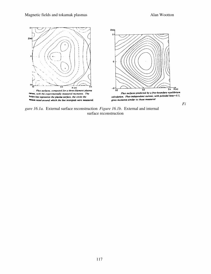
Magnetic fields and tokamak plasmas Alan Wootton
117
Fi
gure 16.1a. External surface reconstruction Figure 16.1b. External and internal
surface reconstruction
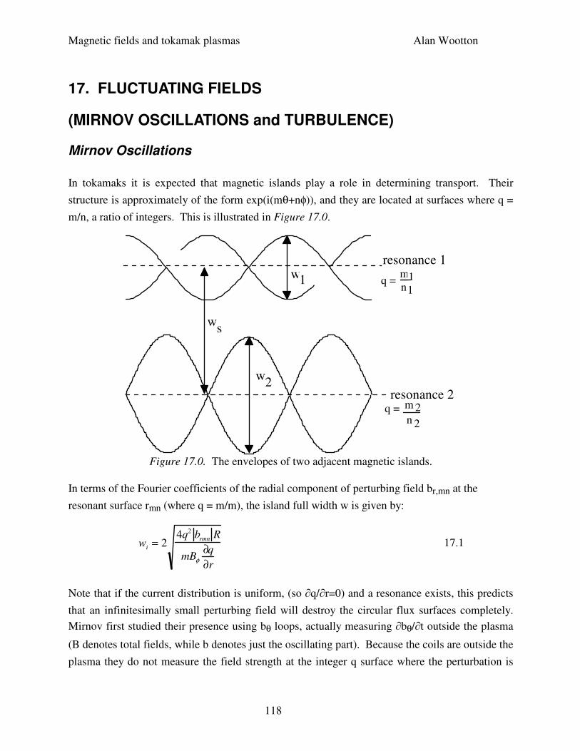
Magnetic fields and tokamak plasmas Alan Wootton
118
17. FLUCTUATING FIELDS
(MIRNOV OSCILLATIONS and TURBULENCE)
Mirnov Oscillations
In tokamaks it is expected that magnetic islands play a role in determining transport. Their
structure is approximately of the form exp(i(mθ+nφ)), and they are located at surfaces where q =
m/n, a ratio of integers. This is illustrated in Figure 17.0.
resonance 1
resonance 2
q =m1n1
m1n1
q = m 2n 2
w2
w1
ws
Figure 17.0. The envelopes of two adjacent magnetic islands.
In terms of the Fourier coefficients of the radial component of perturbing field br,mn at the
resonant surface rmn (where q = m/m), the island full width w is given by:
wi = 24q2 brmn R
mBφ∂q
∂r
17.1
Note that if the current distribution is uniform, (so ∂q/∂r=0) and a resonance exists, this predicts
that an infinitesimally small perturbing field will destroy the circular flux surfaces completely.
Mirnov first studied their presence using bθ loops, actually measuring ∂bθ/∂t outside the plasma
(B denotes total fields, while b denotes just the oscillating part). Because the coils are outside the
plasma they do not measure the field strength at the integer q surface where the perturbation is
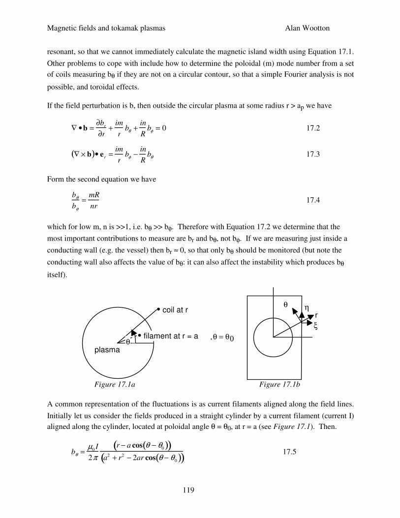
Magnetic fields and tokamak plasmas Alan Wootton
119
resonant, so that we cannot immediately calculate the magnetic island width using Equation 17.1.
Other problems to cope with include how to determine the poloidal (m) mode number from a set
of coils measuring bθ if they are not on a circular contour, so that a simple Fourier analysis is not
possible, and toroidal effects.
If the field perturbation is b, then outside the circular plasma at some radius r > ap we have
∇ •b =∂b
r
∂r+
im
rbθ +
in
Rbφ = 0 17.2
∇ × b( )• er =im
rbφ −
in
Rbθ 17.3
Form the second equation we have
bθ
bφ
=mR
nr 17.4
which for low m, n is >>1, i.e. bθ >> bφ. Therefore with Equation 17.2 we determine that the
most important contributions to measure are br and bθ, not bφ. If we are measuring just inside a
conducting wall (e.g. the vessel) then br ≈ 0, so that only bθ should be monitored (but note the
conducting wall also affects the value of bθ: it can also affect the instability which produces bθ
itself).
•
coil at r
filament at r = a
plasma
•
θθ = θ0,
ξ
ηr
θ
Figure 17.1a Figure 17.1b
A common representation of the fluctuations is as current filaments aligned along the field lines.
Initially let us consider the fields produced in a straight cylinder by a current filament (current I)
aligned along the cylinder, located at poloidal angle θ = θ0, at r = a (see Figure 17.1). Then.
bθ =µ0 I
2π
r − a cos θ − θ0( )( )a2 + r2 − 2ar cos θ − θ0( )( ) 17.5
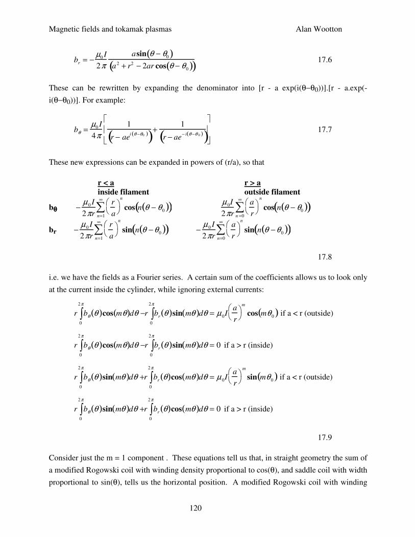
Magnetic fields and tokamak plasmas Alan Wootton
120
br = −µ0 I
2πasin θ − θ0( )
a2 + r2 − 2ar cos θ − θ0( )( ) 17.6
These can be rewritten by expanding the denominator into [r - a exp(i(θ−θ0))].[r - a.exp(-
i(θ−θ0))]. For example:
bθ =µ0 I
4π1
r − aei θ −θ0( )( )+
1
r − ae− i θ −θ 0( )( )
17.7
These new expressions can be expanded in powers of (r/a), so that
r < a r > a
inside filament outside filament
bθθθθ −µ0 I
2πr
r
a
n=1
∞
∑n
cos n θ − θ0( )( ) µ 0I
2πr
a
r
n =0
∞
∑n
cos n θ − θ0( )( )
br −µ0 I
2πr
r
a
n=1
∞
∑n
sin n θ −θ0( )( ) −µ0 I
2πr
a
r
n=0
∞
∑n
sin n θ −θ0( )( )
17.8
i.e. we have the fields as a Fourier series. A certain sum of the coefficients allows us to look only
at the current inside the cylinder, while ignoring external currents:
r bθ θ( )cos mθ( )dθ −0
2π
∫ r br θ( )sin mθ( )dθ = µ0I0
2π
∫a
r
m
cos mθ0( ) if a < r (outside)
r bθ θ( )cos mθ( )dθ −0
2π
∫ r br θ( )sin mθ( )dθ = 00
2π
∫ if a > r (inside)
r bθ θ( )sin mθ( )dθ +0
2π
∫ r br θ( )cos mθ( )dθ = µ 0I0
2π
∫a
r
m
sin mθ0( ) if a < r (outside)
r bθ θ( )sin mθ( )dθ +0
2π
∫ r br θ( )cos mθ( )dθ = 00
2π
∫ if a > r (inside)
17.9
Consider just the m = 1 component . These equations tell us that, in straight geometry the sum of
a modified Rogowski coil with winding density proportional to cos(θ), and saddle coil with width
proportional to sin(θ), tells us the horizontal position. A modified Rogowski coil with winding
Magnetic fields and tokamak plasmas Alan Wootton
121
density proportional to sin(θ), and saddle coil with width proportional to cos(θ), tells us the
vertical position. Actually we already new this; section 9 tells us how to do better and correct for
toroidal effects as well. Note if the Mirnov coils are mounted just inside a conducting vessel then
br = 0, and the second terms are zero.
Now we must consider a general distribution j(r,θ) instead of the line current at r = a. Then using
complex notation, and assuming a conducting vessel where br = 0:
r bθ θ( )0
2π
∫ eimθ
dθ = µ 0 dr'0
r
∫r'
r
m
r' dθj r' ,θ( )0
2π
∫ eimθ
17.10
thus relating moments of the external field to moments of the current density. Rogowski coils
with winding density cos(mθ) and sin(mθ) would directly measure the LHS of this equation
(again we knew this from section 9). Now we see a problem: the LHS is an integral over θ while
the RHS is an integral over r’ and θ. Without some assumptions we cannot work back from the
externally measured fields to the currents at the surface. This is exactly the same problem that
we came across in dealing with reconstructing the plasma shape from the multipole moments
without invoking equilibrium: varying the assumed jφ distribution gives different plasma shapes.
A typical assumption is
j r,θ( )= j0 r( ) + jmnem ,n
∑i mθ +nφ −ω mn t( )
δ r − rmn( ) 17.11
with j0(r) the equilibrium current, rmn the radius of the resonant surface, δ(r-rmn) the delta
function restricting the currents to r = rmn. The perturbed field measured at r, produced by the
current perturbation jmn at rmn, is
bθ r ,θ,φ( ) = µ 0 jmnrmn
rmn
r
m +1
ei mθ +nφ −ω mn t( )
for r > rmn 17.12
Here we have introduced a frequency f = ω/(2π) into the problem: the filaments are rotating. If
we want to consider br and bθ, and work in real space, then
bθ =µ0 jmnrmn
2
rmn
r
m +1
cos mθ + nφ − ωmnt( ) 17.13
br = −µ0 jmnrmn
2
rmn
r
m +1
sin mθ + nφ − ωmnt( ) 17.14
Magnetic fields and tokamak plasmas Alan Wootton
122
Often we will write an expression for the Fourier coefficients of the field at the resonant surface,
bmn r = rmn( )= µ0 jmnrmn
2 . Note if we were working on a rectangular vessel we would measure
for example bη (see Figure 10.1):
bη = bθ cos θ( )+ br sin θ( ) = bmn
rmn
r
m +1
cos m +1( )θ + nφ − ωmnt( ) 17.15
i.e. we see that working with a rectangular contour the phase varies as (m+1)θ, instead of mθ
when working with a circular contour.
Now in toroidal geometry there are complications. We must consider that
a) jmn produces a stronger field at the inner equator
b) the perturbation are displaced because of a Shafranov shift
c) the pitch of the field lines is no longer constant
We will now derive the toroidal corrections for a case where we are considering surface current
perturbations for our model equilibrium of section 6. We start with the field line equation for the
total equilibrium fields, evaluated at a radius r = ap, the plasma minor radius:
adθBθ
=RdφBφ
17.16
With
R = Rg + acos θ( ) 17.17
Bφ =Bφ 0(R = Rg )
1 + a
Rg
cos θ( )
17.18
Bθa =µ 0 I
p
2πa1 +
a
Rg
ΛΛΛΛcos θ( )
17.19
ΛΛΛΛ = β I +li
2−1 17.20
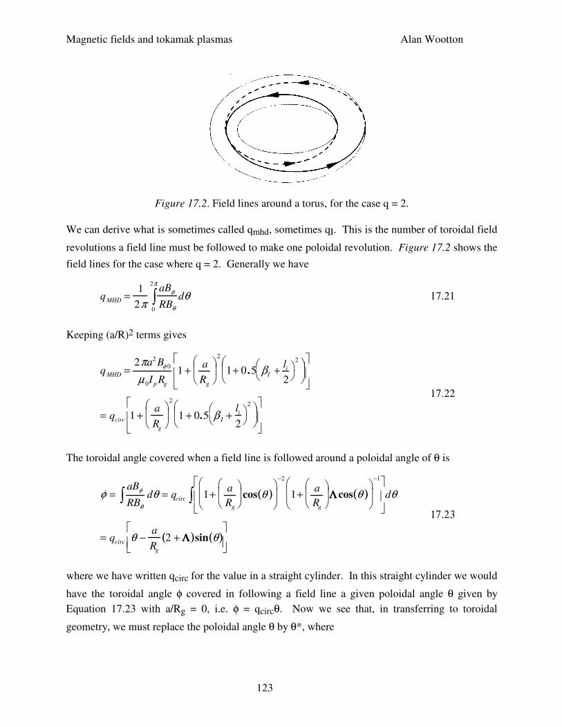
Magnetic fields and tokamak plasmas Alan Wootton
123
Figure 17.2. Field lines around a torus, for the case q = 2.
We can derive what is sometimes called qmhd, sometimes qI. This is the number of toroidal field
revolutions a field line must be followed to make one poloidal revolution. Figure 17.2 shows the
field lines for the case where q = 2. Generally we have
qMHD =1
2πaBφ
RBθ
dθ0
2π
∫ 17.21
Keeping (a/R)2 terms gives
qMHD =2πa2 Bφ 0
µ 0I p Rg
1 + a
Rg
2
1+ 0 .5 βI + li
2
2
= qcirc 1 +a
Rg
2
1 + 0.5 β I +li
2
2
17.22
The toroidal angle covered when a field line is followed around a poloidal angle of θ is
φ =aBφ
RBθ
dθ∫ = qcirc 1+ a
Rg
cos θ( )
−2
1+ a
Rg
ΛΛΛΛ cos θ( )
−1
dθ∫
= qcirc θ −a
Rg
2 + ΛΛΛΛ( )sin θ( )
17.23
where we have written qcirc for the value in a straight cylinder. In this straight cylinder we would
have the toroidal angle φ covered in following a field line a given poloidal angle θ given by
Equation 17.23 with a/Rg = 0, i.e. φ = qcircθ. Now we see that, in transferring to toroidal
geometry, we must replace the poloidal angle θ by θ*, where
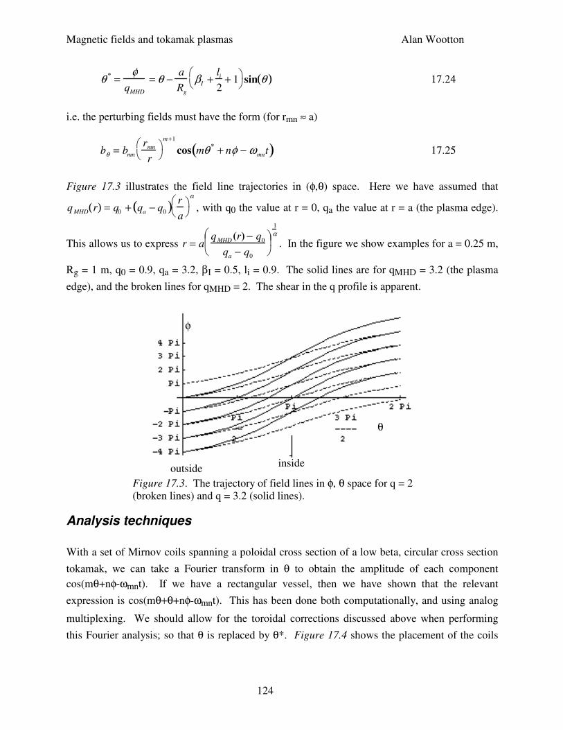
Magnetic fields and tokamak plasmas Alan Wootton
124
θ * =φ
qMHD
= θ −a
Rg
βI +li
2+ 1
sin θ( ) 17.24
i.e. the perturbing fields must have the form (for rmn ≈ a)
bθ = bmn
rmn
r
m +1
cos mθ * + nφ − ωmnt( ) 17.25
Figure 17.3 illustrates the field line trajectories in (φ,θ) space. Here we have assumed that
qMHD r( ) = q0 + qa − q0( ) r
a
α
, with q0 the value at r = 0, qa the value at r = a (the plasma edge).
This allows us to express r = aqMHD (r) − q0
qa − q0
1
α
. In the figure we show examples for a = 0.25 m,
Rg = 1 m, q0 = 0.9, qa = 3.2, βI = 0.5, li = 0.9. The solid lines are for qMHD = 3.2 (the plasma
edge), and the broken lines for qMHD = 2. The shear in the q profile is apparent.
φ
θ
outsideinside
Figure 17.3. The trajectory of field lines in φ, θ space for q = 2
(broken lines) and q = 3.2 (solid lines).
Analysis techniques
With a set of Mirnov coils spanning a poloidal cross section of a low beta, circular cross section
tokamak, we can take a Fourier transform in θ to obtain the amplitude of each component
cos(mθ+nφ-ωmnt). If we have a rectangular vessel, then we have shown that the relevant
expression is cos(mθ+θ+nφ-ωmnt). This has been done both computationally, and using analog
multiplexing. We should allow for the toroidal corrections discussed above when performing
this Fourier analysis; so that θ is replaced by θ*. Figure 17.4 shows the placement of the coils
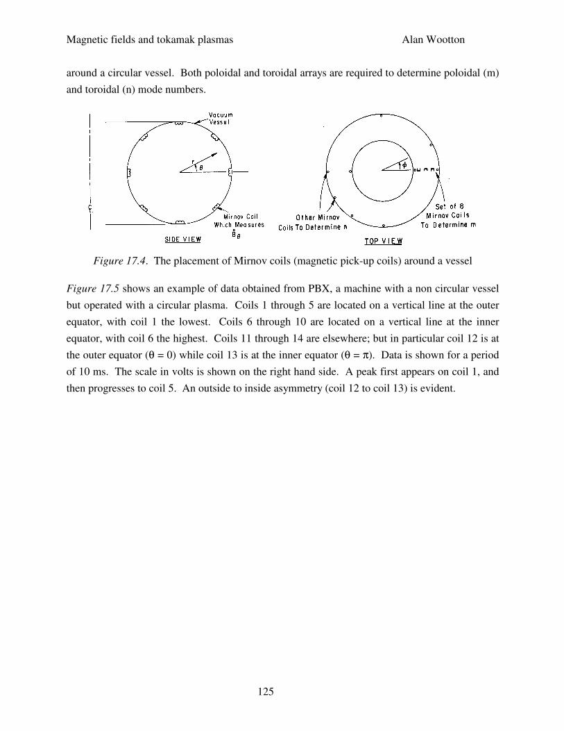
Magnetic fields and tokamak plasmas Alan Wootton
125
around a circular vessel. Both poloidal and toroidal arrays are required to determine poloidal (m)
and toroidal (n) mode numbers.
Figure 17.4. The placement of Mirnov coils (magnetic pick-up coils) around a vessel
Figure 17.5 shows an example of data obtained from PBX, a machine with a non circular vessel
but operated with a circular plasma. Coils 1 through 5 are located on a vertical line at the outer
equator, with coil 1 the lowest. Coils 6 through 10 are located on a vertical line at the inner
equator, with coil 6 the highest. Coils 11 through 14 are elsewhere; but in particular coil 12 is at
the outer equator (θ = 0) while coil 13 is at the inner equator (θ = π). Data is shown for a period
of 10 ms. The scale in volts is shown on the right hand side. A peak first appears on coil 1, and
then progresses to coil 5. An outside to inside asymmetry (coil 12 to coil 13) is evident.
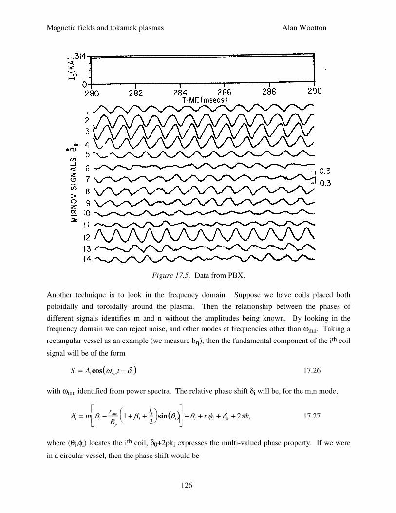
Magnetic fields and tokamak plasmas Alan Wootton
126
Figure 17.5. Data from PBX.
Another technique is to look in the frequency domain. Suppose we have coils placed both
poloidally and toroidally around the plasma. Then the relationship between the phases of
different signals identifies m and n without the amplitudes being known. By looking in the
frequency domain we can reject noise, and other modes at frequencies other than ωmn. Taking a
rectangular vessel as an example (we measure bη), then the fundamental component of the ith coil
signal will be of the form
Si = Ai cos ωmnt − δ i( ) 17.26
with ωmn identified from power spectra. The relative phase shift δi will be, for the m,n mode,
δ i = m θi −rmn
Rg
1 +β I +li
2
sin θ i( )
+θ i + nφ i + δ0 + 2πki 17.27
where (θi,φi) locates the ith coil, δ0+2pki expresses the multi-valued phase property. If we were
in a circular vessel, then the phase shift would be
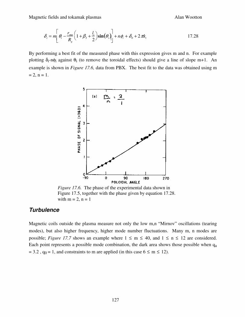
Magnetic fields and tokamak plasmas Alan Wootton
127
δ i = m θi −rmn
Rg
1 +β I +li
2
sin θ i( )
+ nφi + δ0 + 2πki 17.28
By performing a best fit of the measured phase with this expression gives m and n. For example
plotting δi-nφi against θi (to remove the toroidal effects) should give a line of slope m+1. An
example is shown in Figure 17.6, data from PBX. The best fit to the data was obtained using m
= 2, n = 1.
Figure 17.6. The phase of the experimental data shown in
Figure 17.5, together with the phase given by equation 17.28.
with m = 2, n = 1
Turbulence
Magnetic coils outside the plasma measure not only the low m,n “Mirnov” oscillations (tearing
modes), but also higher frequency, higher mode number fluctuations. Many m, n modes are
possible; Figure 17.7 shows an example where 1 ≤ m ≤ 40, and 1 ≤ n ≤ 12 are considered.
Each point represents a possible mode combination, the dark area shows those possible when qa
= 3.2 , q0 = 1, and constraints to m are applied (in this case 6 ≤ m ≤ 12).
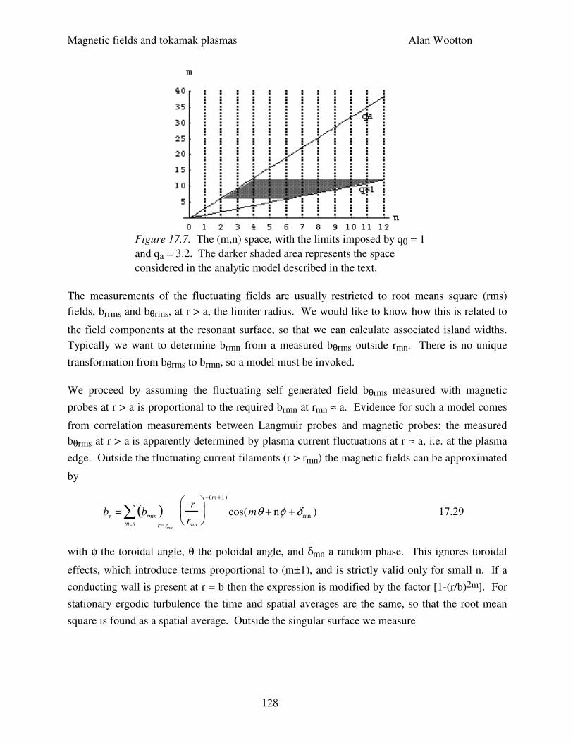
Magnetic fields and tokamak plasmas Alan Wootton
128
Figure 17.7. The (m,n) space, with the limits imposed by q0 = 1
and qa = 3.2. The darker shaded area represents the space
considered in the analytic model described in the text.
The measurements of the fluctuating fields are usually restricted to root means square (rms)
fields, brrms and bθrms, at r > a, the limiter radius. We would like to know how this is related to
the field components at the resonant surface, so that we can calculate associated island widths.
Typically we want to determine brmn from a measured bθrms outside rmn. There is no unique
transformation from bθrms to brmn, so a model must be invoked.
We proceed by assuming the fluctuating self generated field bθrms measured with magnetic
probes at r > a is proportional to the required brmn at rmn ≈ a. Evidence for such a model comes
from correlation measurements between Langmuir probes and magnetic probes; the measured
bθrms at r > a is apparently determined by plasma current fluctuations at r ≈ a, i.e. at the plasma
edge. Outside the fluctuating current filaments (r > rmn) the magnetic fields can be approximated
by
br = brmn( )m ,n
∑r= rmn
r
rmn
−(m +1)
cos(mθ + nφ +δmn ) 17.29
with φ the toroidal angle, θ the poloidal angle, and δmn a random phase. This ignores toroidal
effects, which introduce terms proportional to (m±1), and is strictly valid only for small n. If a
conducting wall is present at r = b then the expression is modified by the factor [1-(r/b)2m]. For
stationary ergodic turbulence the time and spatial averages are the same, so that the root mean
square is found as a spatial average. Outside the singular surface we measure
Magnetic fields and tokamak plasmas Alan Wootton
129
brms = br ,rms = bθ ,rms = 0.5 brmn r= rmn
2 r
rmn
−2(m +1)
m ,n
∑ 17.30
To go further and obtain a relationship between bθrms at r > a in terms of brmn at r = rmn we must
specify
a given current density or safety factor profile q(r),
the dependence of brmn on m and n,
locate all possible m and n pairs where q = m/n,
specify upper and lower limits to either m or n.
In general this must be done computationally. However, some progress can be made analytically.
We can approximately solve Equation 17.30 for bθrms at r > a in terms of brmn at r = rmn if we
take brmn independent of m and n over some range to be specified, and a q profile relevant to the
plasma edge, for example q = qa
r
a
2
. Then we can relate the resonance location rmn to a given
q,
rmn
a=
q
qa
1
2
=m
nqa
1
2
17.31
With ρ = r/a defining the measurement position and q = m/n, Equation 17.30 is written as
brms
brmn
ρ ≥1
2
= 0.51
ρ
2(m+1)
m
nqa
(m +1)
m ,n
∑ 17.32
ρ ≥ 1 is a constant, namely the location of the magnetic pick-up coils used to measure brms.
We now replace the summation by integrals. The space we are considering is shown in Figure
17.4. The first integral, ∫dn, is from m/qa to m, allowing all n values in between. The second
integral, ∫dm, is from m1 to m2, with m2 >> m1. In Figure 17.4 m1 = 6 and m2 = 12.
Unfortunately our chosen profile allows q ≤ 1 (when rmn/a ≤ 1/√qa). To restrict n ≥ 1 we should
choose m1 ≥ qa ≈ 3. The result of the integration is
brms
brmn
=
1
4qa ln ρ( )1
ρ2 m1 +1( ) −1
ρ 2 m2 +1( )
−1
2 ln qa( )+ 2 ln ρ( )( )1
qa
m1 +1( )ρ 2 m1+1( ) −1
qa
m 2+1( )ρ2 m 2+1( )
1
2
Magnetic fields and tokamak plasmas Alan Wootton
130
17.33
This expression can be further simplified for ρ > 1 by noting m2 >> 1 (so all terms involving m2
disappear) and m1 > 1 (so the term involving qa(m1+1) disappears) to give
brms
brmn
=1
2ρ m1 +1( ) qa ln ρ( ) 17.34
This is the required result, giving us brmn at the plasma edge in terms of the measured brms
outside the plasma. Because the terms involving m2 have been ignored in deriving Equation
17.34 it predicts (brms/|brmn|)ρ⇒1 ⇒ ∞. The more complete expression, remains finite, and
brms
brmn
r= a
≈m2 − m1( )
2qa
17.35
We conclude that the measured rms field outside the plasma (ρ > 1) is determined only by the
lowest m number (m1); the higher m numbers fall off too rapidly to contribute. Indeed, if
Equation 17.34 is taken to represent the results, then a fit of the form brms ∝ r-γ gives the result
γ = m1 + 1+1
2 ln ρ( ) 17.36
We can also measure the frequency of the fluctuations. We assume that the observed frequency
is described by an expression of the form
f =ω2π
=m
2πrmn Bφ
κTe
e ne
∂ne
∂r− Er
17.37
This is consistent with experimental results, with κ a factor of order 1. We also know
experimentally that the term involving Er dominates the term involving κ, and that we can
approximate the expression by
f ≈−cmEr
2πrmnBφ
17.38
with χ a factor ≈ 1.5. Er is approximately constant for ρ < 1. We now relate rmn to q = m/n by
assuming a specific q profile. For the simple q profile used in deriving the analytic results the
transformation from rmn to m and n is given by Equation 17.31. A more realistic q profile gives
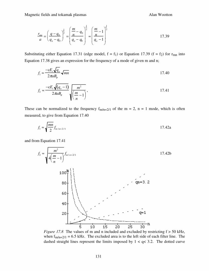
Magnetic fields and tokamak plasmas Alan Wootton
131
rmn
a=
q − q0
qa − q0
1
2
=
m
n− q0
qa − q0
1
2
≈
m
n−1
qa −1
1
2
17.39
Substituting either Equation 17.31 (edge model, f = f1) or Equation 17.39 (f = f2) for rmn into
Equation 17.38 gives an expression for the frequency of a mode of given m and n;
f1 ≈−cEr qa
2πaBφ
mn 17.40
f2 ≈−cEr qa −1( )
2πaBφ
m2
m
n−1
, 17.41
These can be normalized to the frequency fm/n=2/1 of the m = 2, n = 1 mode, which is often
measured, to give from Equation 17.40
f1 ≈mn
2fm / n= 2 / 1 17.42a
and from Equation 17.41
f2 ≈m2
4m
n−1
fm / n= 2/ 1 17.42b
Figure 17.8 The values of m and n included and excluded by restricting f > 50 kHz,
when fm/n=2/1 = 6.5 kHz. The excluded area is to the left side of each filter line. The
dashed straight lines represent the limits imposed by 1 < q< 3.2. The dotted curve
Magnetic fields and tokamak plasmas Alan Wootton
132
represents the limits imposed by the frequency filter from Equation 17.42a and
Equation 17.42b.
If only modes with f > fmin are considered, we can derive mlim, a function of fmin/fm/n=2/1 and n,
which separates modes which are and are not included in any subsequent analysis. The results
are shown in Figure 17.8 for fmin = 50kHz, fm/n=2/1 = 6.5 kHz. In general, frequency filtering
should be considered more a restriction on n than on m.
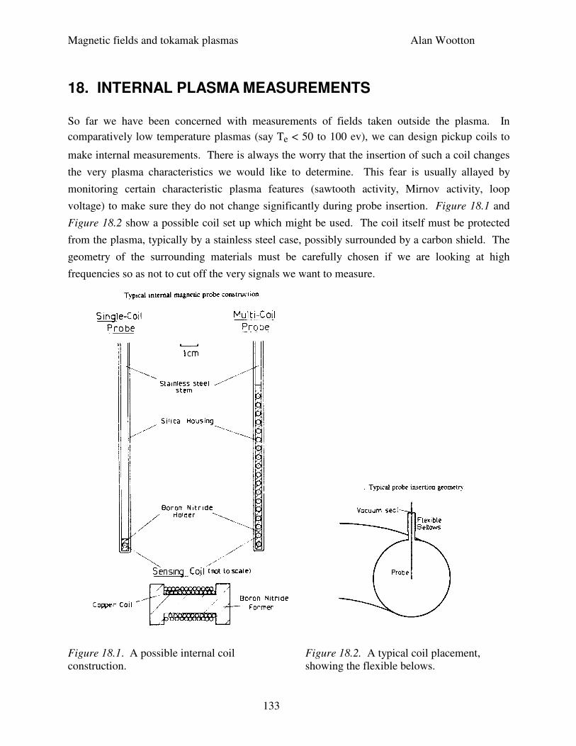
Magnetic fields and tokamak plasmas Alan Wootton
133
18. INTERNAL PLASMA MEASUREMENTS
So far we have been concerned with measurements of fields taken outside the plasma. In
comparatively low temperature plasmas (say Te < 50 to 100 ev), we can design pickup coils to
make internal measurements. There is always the worry that the insertion of such a coil changes
the very plasma characteristics we would like to determine. This fear is usually allayed by
monitoring certain characteristic plasma features (sawtooth activity, Mirnov activity, loop
voltage) to make sure they do not change significantly during probe insertion. Figure 18.1 and
Figure 18.2 show a possible coil set up which might be used. The coil itself must be protected
from the plasma, typically by a stainless steel case, possibly surrounded by a carbon shield. The
geometry of the surrounding materials must be carefully chosen if we are looking at high
frequencies so as not to cut off the very signals we want to measure.
Figure 18.1. A possible internal coil Figure 18.2. A typical coil placement,
construction. showing the flexible belows.
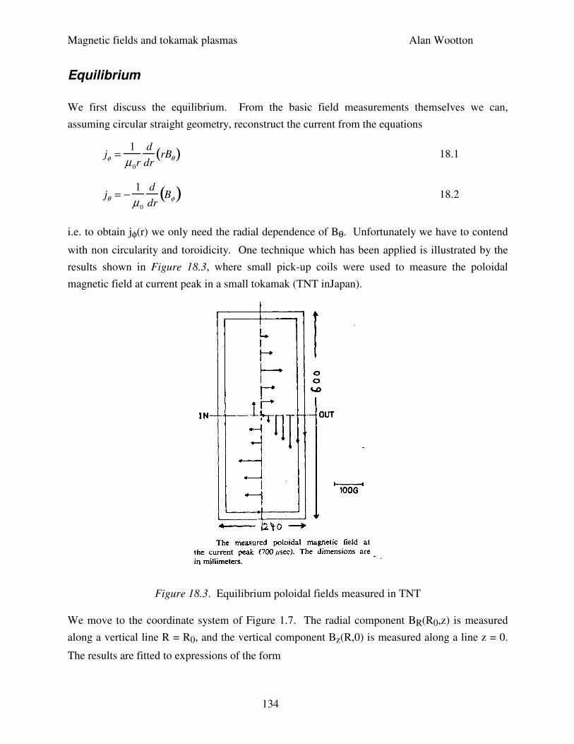
Magnetic fields and tokamak plasmas Alan Wootton
134
Equilibrium
We first discuss the equilibrium. From the basic field measurements themselves we can,
assuming circular straight geometry, reconstruct the current from the equations
jφ =1
µ 0r
d
drrBθ( ) 18.1
jθ = −1
µ 0
d
drBφ( ) 18.2
i.e. to obtain jφ(r) we only need the radial dependence of Bθ. Unfortunately we have to contend
with non circularity and toroidicity. One technique which has been applied is illustrated by the
results shown in Figure 18.3, where small pick-up coils were used to measure the poloidal
magnetic field at current peak in a small tokamak (TNT inJapan).
Figure 18.3. Equilibrium poloidal fields measured in TNT
We move to the coordinate system of Figure 1.7. The radial component BR(R0,z) is measured
along a vertical line R = R0, and the vertical component Bz(R,0) is measured along a line z = 0.
The results are fitted to expressions of the form
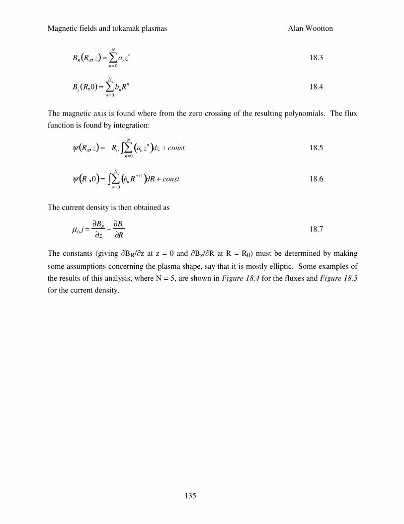
Magnetic fields and tokamak plasmas Alan Wootton
135
BR R0, z( )= an
n= 0
N
∑ zn 18.3
Bz R,0( ) = bnRn
n= 0
N
∑ 18.4
The magnetic axis is found where from the zero crossing of the resulting polynomials. The flux
function is found by integration:
ψ R0, z( ) = −R0 an zn( )dz
n=0
N
∑∫ + const 18.5
ψ R ,0( )= bn Rn+1( )dR
n= 0
N
∑∫ + const 18.6
The current density is then obtained as
µ 0 j =∂B
R
∂z−
∂Bz
∂R 18.7
The constants (giving ∂BR/∂z at z = 0 and ∂Bz/∂R at R = R0) must be determined by making
some assumptions concerning the plasma shape, say that it is mostly elliptic. Some examples of
the results of this analysis, where N = 5, are shown in Figure 18.4 for the fluxes and Figure 18.5
for the current density.
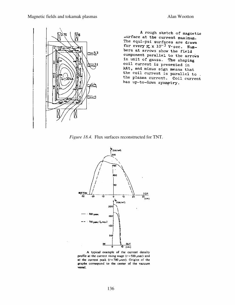
Magnetic fields and tokamak plasmas Alan Wootton
136
Figure 18.4. Flux surfaces reconstructed for TNT.
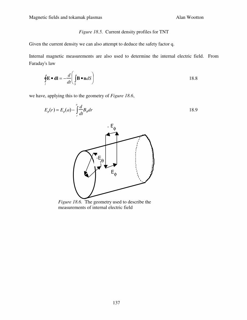
Magnetic fields and tokamak plasmas Alan Wootton
137
Figure 18.5. Current density profiles for TNT
Given the current density we can also attempt to deduce the safety factor q.
Internal magnetic measurements are also used to determine the internal electric field. From
Faraday's law
E • dl = −d
dtl
∫ B •ndSS
∫
18.8
we have, applying this to the geometry of Figure 18.6,
Eφ r( ) = Eφ a( ) −d
dtr
a
∫ Bθ dr 18.9
E
Eφ
φ
-
-Eθ
Figure 18.6. The geometry used to describe the
measurements of internal electric field
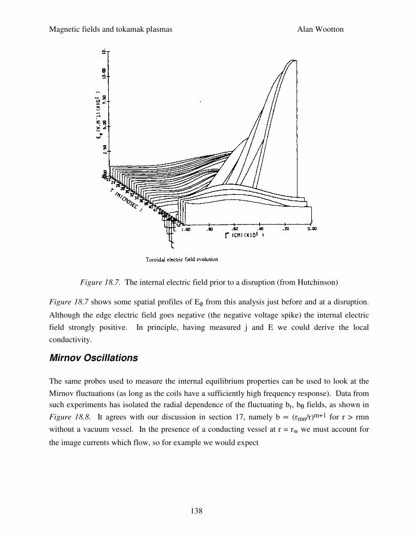
Magnetic fields and tokamak plasmas Alan Wootton
138
Figure 18.7. The internal electric field prior to a disruption (from Hutchinson)
Figure 18.7 shows some spatial profiles of Eφ from this analysis just before and at a disruption.
Although the edge electric field goes negative (the negative voltage spike) the internal electric
field strongly positive. In principle, having measured j and E we could derive the local
conductivity.
Mirnov Oscillations
The same probes used to measure the internal equilibrium properties can be used to look at the
Mirnov fluctuations (as long as the coils have a sufficiently high frequency response). Data from
such experiments has isolated the radial dependence of the fluctuating br, bθ fields, as shown in
Figure 18.8. It agrees with our discussion in section 17, namely b ∝ (rmn/r)m+1 for r > rmn
without a vacuum vessel. In the presence of a conducting vessel at r = rw we must account for
the image currents which flow, so for example we would expect
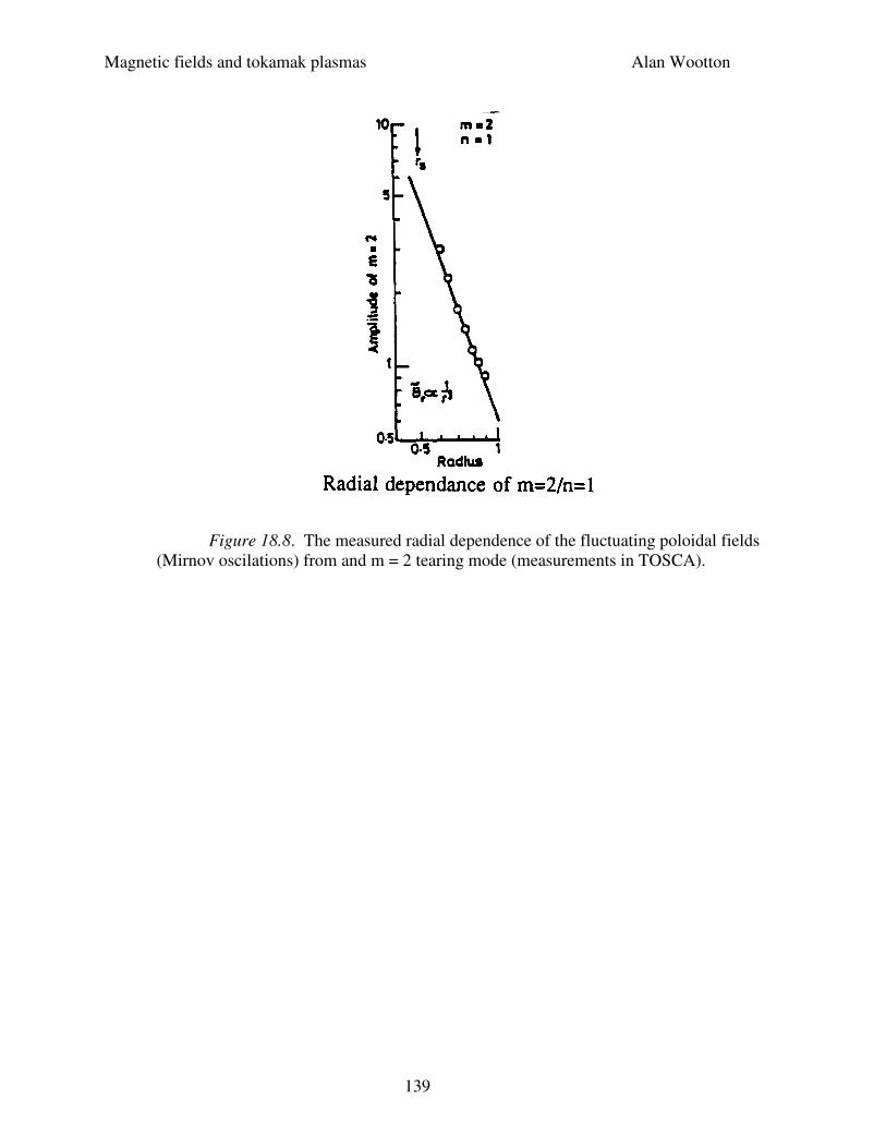
Magnetic fields and tokamak plasmas Alan Wootton
139
Figure 18.8. The measured radial dependence of the fluctuating poloidal fields
(Mirnov oscilations) from and m = 2 tearing mode (measurements in TOSCA).
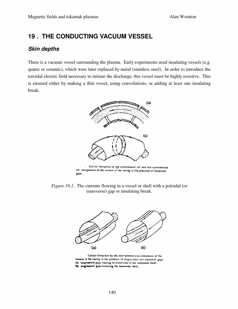
Magnetic fields and tokamak plasmas Alan Wootton
140
19 . THE CONDUCTING VACUUM VESSEL
Skin depths
There is a vacuum vessel surrounding the plasma. Early experiments used insulating vessels (e.g.
quartz or ceramic), which were later replaced by metal (stainless steel). In order to introduce the
toroidal electric field necessary to initiate the discharge, this vessel must be highly resistive. This
is ensured either by making a thin vessel, using convolutions, or adding at least one insulating
break.
Figure 19.1. The currents flowing in a vessel or shell with a poloidal (or
transverse) gap or insulating break.
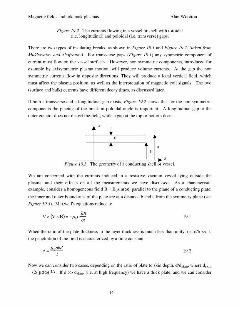
Magnetic fields and tokamak plasmas Alan Wootton
141
Figure 19.2. The currents flowing in a vessel or shell with toroidal
(i.e. longitudinal) and poloidal (i.e. transverse) gaps.
There are two types of insulating breaks, as shown in Figure 19.1 and Figure 19.2, (taken from
Mukhovatov and Shafranov). For transverse gaps (Figure 19.1) any symmetric component of
current must flow on the vessel surfaces. However, non symmetric components, introduced for
example by axisymmetric plasma motion, will produce volume currents. At the gap the non
symmetric currents flow in opposite directions. They will produce a local vertical field, which
must affect the plasma position, as well as the interpretation of magnetic coil signals. The two
(surface and bulk) currents have different decay times, as discussed later.
If both a transverse and a longitudinal gap exists, Figure 19.2 shows that for the non symmetric
components the placing of the break in poloidal angle is important. A longitudinal gap at the
outer equator does not distort the field, while a gap at the top or bottom does.
z
ba
d
x
Figure 19.3. The geometry of a conducting shell or vessel.
We are concerned with the currents induced in a resistive vacuum vessel lying outside the
plasma, and their effects on all the measurements we have discussed. As a characteristic
example, consider a homogeneous field B = B0sin(ωt) parallel to the plane of a conducting plate;
the inner and outer boundaries of the plate are at a distance b and a from the symmetry plane (see
Figure 19.3). Maxwell's equations reduce to
∇ × ∇ × B( ) = −µ0σ∂B
∂t 19.1
When the ratio of the plate thickness to the layer thickness is much less than unity, i.e. d/b << 1,
the penetration of the field is characterized by a time constant
τ =µ 0σbd
2 19.2
Now we can consider two cases, depending on the ratio of plate to skin depth, d/dskin, where dskin
= (2/(µσω))1/2. If d >> dskin, (i.e. at high frequency) we have a thick plate, and we can consider
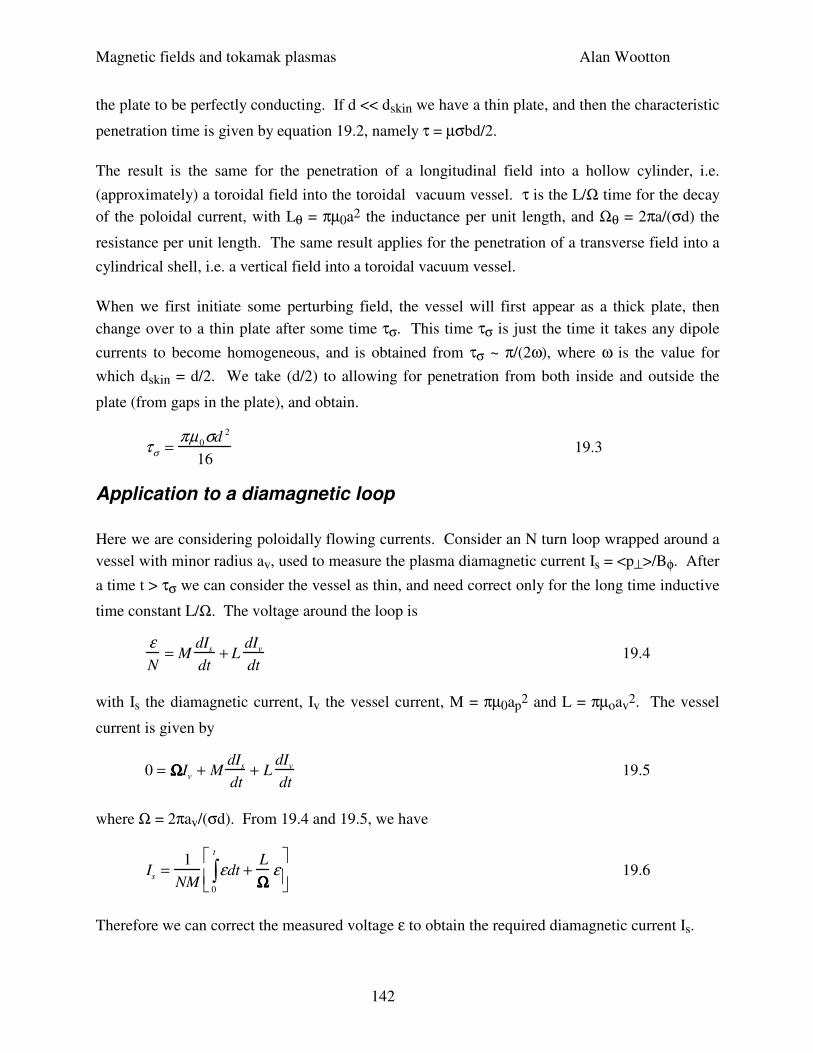
Magnetic fields and tokamak plasmas Alan Wootton
142
the plate to be perfectly conducting. If d << dskin we have a thin plate, and then the characteristic
penetration time is given by equation 19.2, namely τ = µσbd/2.
The result is the same for the penetration of a longitudinal field into a hollow cylinder, i.e.
(approximately) a toroidal field into the toroidal vacuum vessel. τ is the L/Ω time for the decay
of the poloidal current, with Lθ = πµ0a2 the inductance per unit length, and Ωθ = 2πa/(σd) the
resistance per unit length. The same result applies for the penetration of a transverse field into a
cylindrical shell, i.e. a vertical field into a toroidal vacuum vessel.
When we first initiate some perturbing field, the vessel will first appear as a thick plate, then
change over to a thin plate after some time τσ. This time τσ is just the time it takes any dipole
currents to become homogeneous, and is obtained from τσ ~ π/(2ω), where ω is the value for
which dskin = d/2. We take (d/2) to allowing for penetration from both inside and outside the
plate (from gaps in the plate), and obtain.
τσ =πµ0σd 2
16 19.3
Application to a diamagnetic loop
Here we are considering poloidally flowing currents. Consider an N turn loop wrapped around a
vessel with minor radius av, used to measure the plasma diamagnetic current Is = <p⊥>/Bφ. After
a time t > τσ we can consider the vessel as thin, and need correct only for the long time inductive
time constant L/Ω. The voltage around the loop is
εN
= MdIs
dt+ L
dIv
dt 19.4
with Is the diamagnetic current, Iv the vessel current, M = πµ0ap2 and L = πµoav
2. The vessel
current is given by
0 = ΩΩΩΩIv + MdIs
dt+ L
dIv
dt 19.5
where Ω = 2πav/(σd). From 19.4 and 19.5, we have
Is =1
NMεdt +
L
ΩΩΩΩε
0
t
∫
19.6
Therefore we can correct the measured voltage ε to obtain the required diamagnetic current Is.
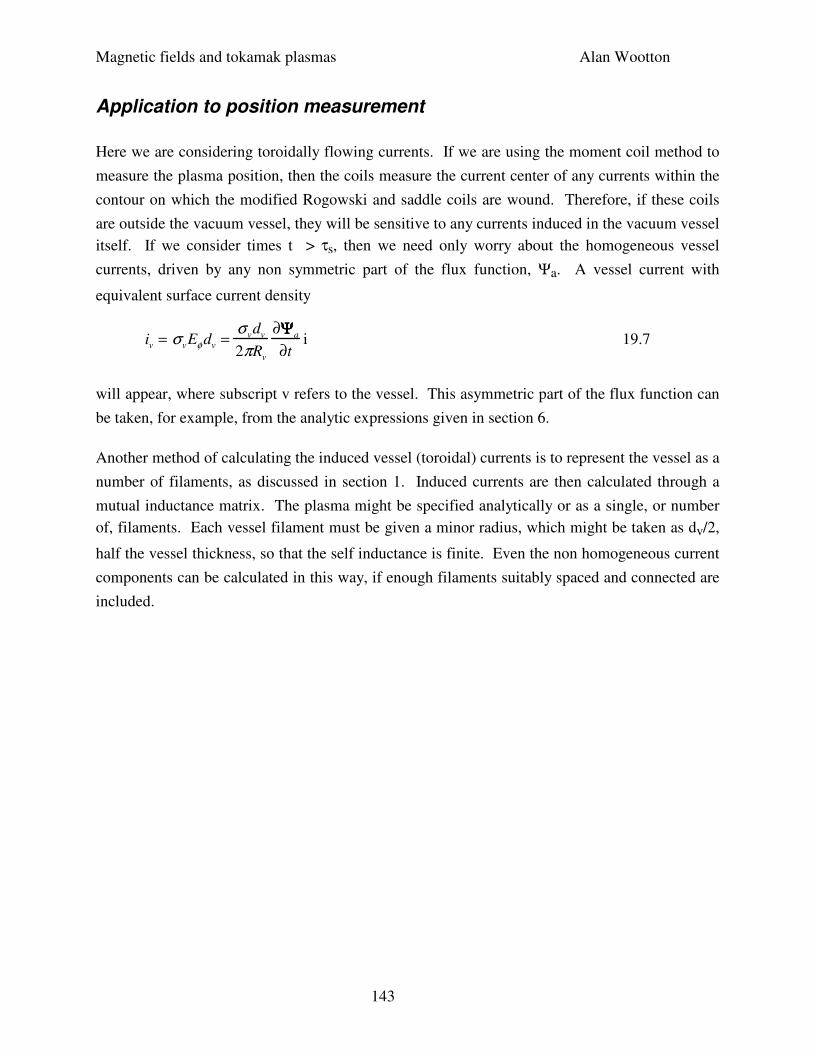
Magnetic fields and tokamak plasmas Alan Wootton
143
Application to position measurement
Here we are considering toroidally flowing currents. If we are using the moment coil method to
measure the plasma position, then the coils measure the current center of any currents within the
contour on which the modified Rogowski and saddle coils are wound. Therefore, if these coils
are outside the vacuum vessel, they will be sensitive to any currents induced in the vacuum vessel
itself. If we consider times t > τs, then we need only worry about the homogeneous vessel
currents, driven by any non symmetric part of the flux function, Ψa. A vessel current with
equivalent surface current density
iv = σvEφ dv =σ
vd
v
2πRv
∂ΨΨΨΨa
∂ti 19.7
will appear, where subscript v refers to the vessel. This asymmetric part of the flux function can
be taken, for example, from the analytic expressions given in section 6.
Another method of calculating the induced vessel (toroidal) currents is to represent the vessel as a
number of filaments, as discussed in section 1. Induced currents are then calculated through a
mutual inductance matrix. The plasma might be specified analytically or as a single, or number
of, filaments. Each vessel filament must be given a minor radius, which might be taken as dv/2,
half the vessel thickness, so that the self inductance is finite. Even the non homogeneous current
components can be calculated in this way, if enough filaments suitably spaced and connected are
included.
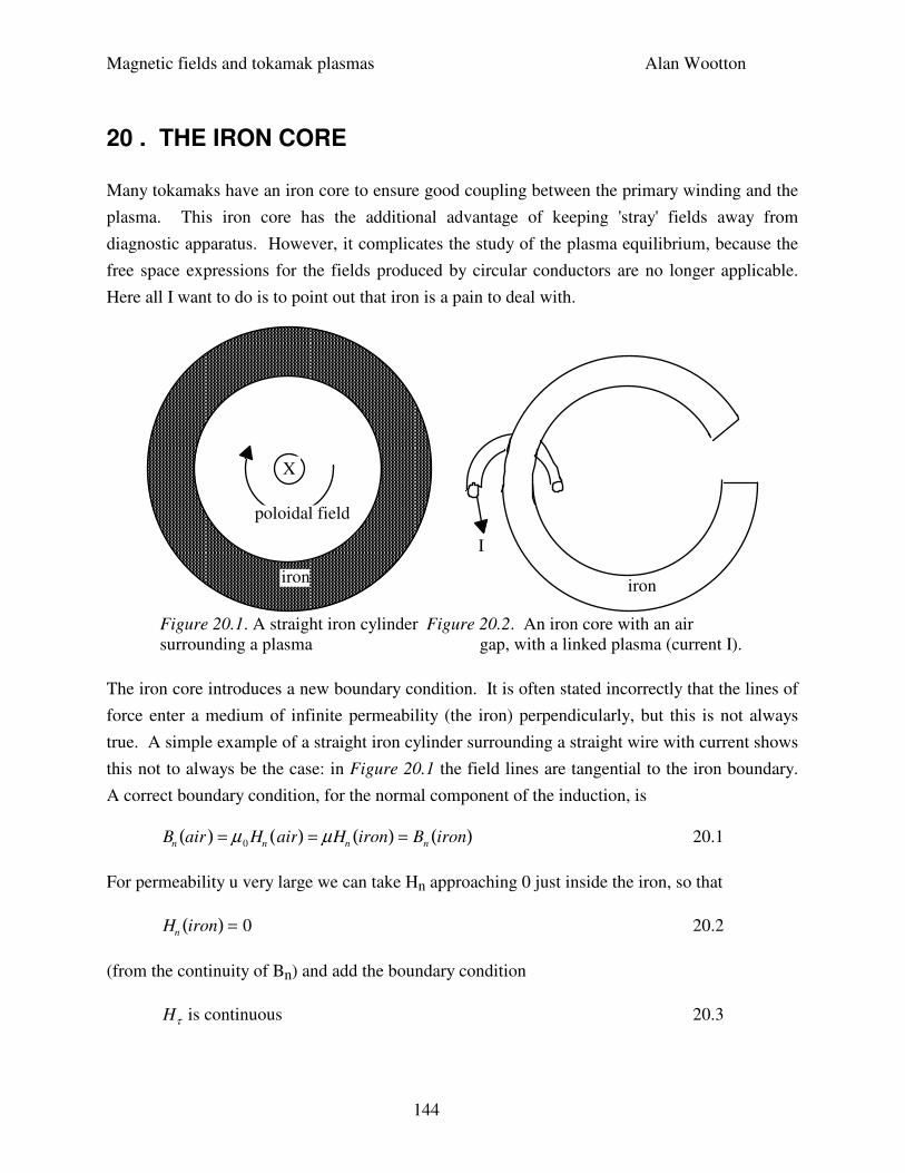
Magnetic fields and tokamak plasmas Alan Wootton
144
20 . THE IRON CORE
Many tokamaks have an iron core to ensure good coupling between the primary winding and the
plasma. This iron core has the additional advantage of keeping 'stray' fields away from
diagnostic apparatus. However, it complicates the study of the plasma equilibrium, because the
free space expressions for the fields produced by circular conductors are no longer applicable.
Here all I want to do is to point out that iron is a pain to deal with.
X
iron
poloidal field
iron
I
Figure 20.1. A straight iron cylinder Figure 20.2. An iron core with an air
surrounding a plasma gap, with a linked plasma (current I).
The iron core introduces a new boundary condition. It is often stated incorrectly that the lines of
force enter a medium of infinite permeability (the iron) perpendicularly, but this is not always
true. A simple example of a straight iron cylinder surrounding a straight wire with current shows
this not to always be the case: in Figure 20.1 the field lines are tangential to the iron boundary.
A correct boundary condition, for the normal component of the induction, is
Bn air( ) = µ 0 Hn air( ) = µHn iron( ) = Bn iron( ) 20.1
For permeability u very large we can take Hn approaching 0 just inside the iron, so that
Hn iron( ) = 0 20.2
(from the continuity of Bn) and add the boundary condition
Hτ is continuous 20.3
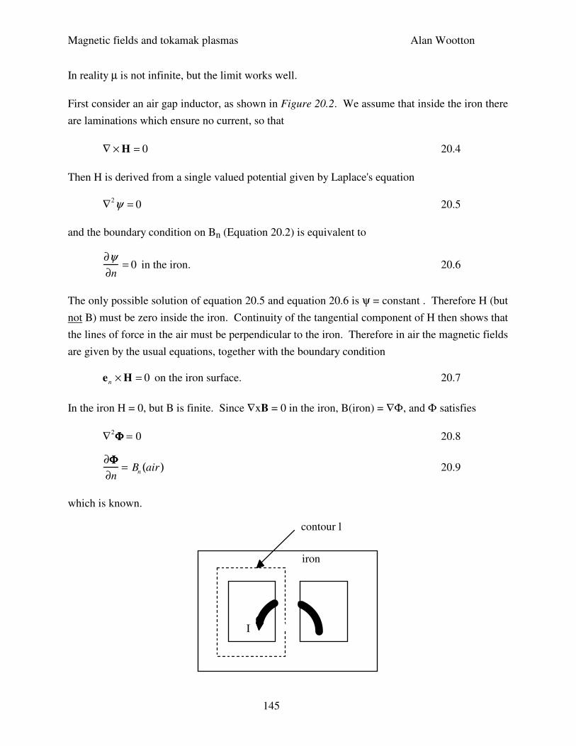
Magnetic fields and tokamak plasmas Alan Wootton
145
In reality µ is not infinite, but the limit works well.
First consider an air gap inductor, as shown in Figure 20.2. We assume that inside the iron there
are laminations which ensure no current, so that
∇ × H = 0 20.4
Then H is derived from a single valued potential given by Laplace's equation
∇2ψ = 0 20.5
and the boundary condition on Bn (Equation 20.2) is equivalent to
∂ψ∂n
= 0 in the iron. 20.6
The only possible solution of equation 20.5 and equation 20.6 is ψ = constant . Therefore H (but
not B) must be zero inside the iron. Continuity of the tangential component of H then shows that
the lines of force in the air must be perpendicular to the iron. Therefore in air the magnetic fields
are given by the usual equations, together with the boundary condition
en × H = 0 on the iron surface. 20.7
In the iron H = 0, but B is finite. Since ∇xB = 0 in the iron, B(iron) = ∇Φ, and Φ satisfies
∇2ΦΦΦΦ = 0 20.8
∂ΦΦΦΦ∂n
= Bn air( ) 20.9
which is known.
contour l
iron
I
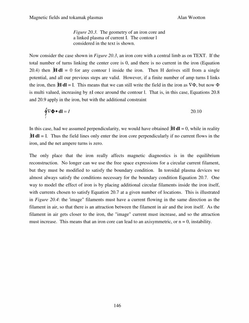
Magnetic fields and tokamak plasmas Alan Wootton
146
Figure 20.3. The geometry of an iron core and
a linked plasma of current I. The contour l
considered in the text is shown.
Now consider the case shown in Figure 20.3, an iron core with a central limb as on TEXT. If the
total number of turns linking the center core is 0, and there is no current in the iron (Equation
20.4) then ∫H.dl = 0 for any contour l inside the iron. Then H derives still from a single
potential, and all our previous steps are valid. However, if a finite number of amp turns I links
the iron, then ∫H.dl = I. This means that we can still write the field in the iron as ∇Φ, but now Φ
is multi valued, increasing by ±I once around the contour l. That is, in this case, Equations 20.8
and 20.9 apply in the iron, but with the additional constraint
∇ΦΦΦΦ • dl = Il
∫ 20.10
In this case, had we assumed perpendicularity, we would have obtained ∫H.dl = 0, while in reality
∫H.dl = I. Thus the field lines only enter the iron core perpendicularly if no current flows in the
iron, and the net ampere turns is zero.
The only place that the iron really affects magnetic diagnostics is in the equilibrium
reconstruction. No longer can we use the free space expressions for a circular current filament,
but they must be modified to satisfy the boundary condition. In toroidal plasma devices we
almost always satisfy the conditions necessary for the boundary condition Equation 20.7. One
way to model the effect of iron is by placing additional circular filaments inside the iron itself,
with currents chosen to satisfy Equation 20.7 at a given number of locations. This is illustrated
in Figure 20.4: the 'image" filaments must have a current flowing in the same direction as the
filament in air, so that there is an attraction between the filament in air and the iron itself. As the
filament in air gets closer to the iron, the "image" current must increase, and so the attraction
must increase. This means that an iron core can lead to an axisymmetric, or n = 0, instability.
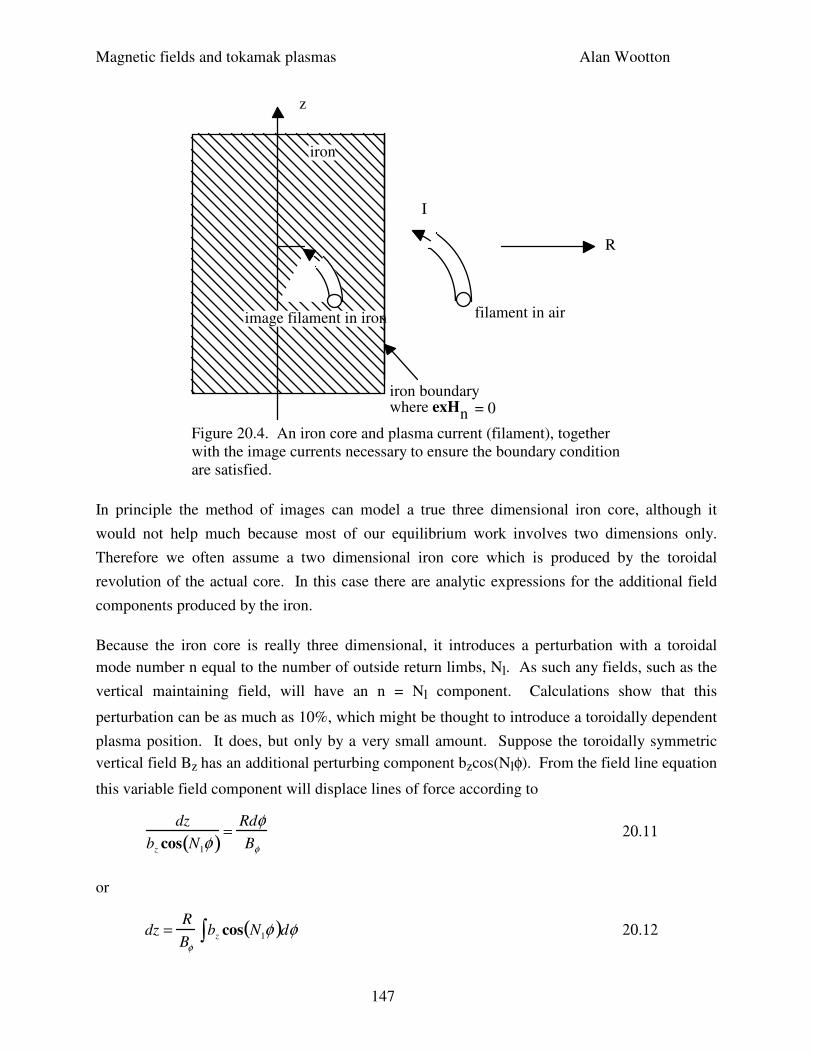
Magnetic fields and tokamak plasmas Alan Wootton
147
z
R
I
filament in air
iron
image filament in iron
iron boundary where exHn = 0
Figure 20.4. An iron core and plasma current (filament), together
with the image currents necessary to ensure the boundary condition
are satisfied.
In principle the method of images can model a true three dimensional iron core, although it
would not help much because most of our equilibrium work involves two dimensions only.
Therefore we often assume a two dimensional iron core which is produced by the toroidal
revolution of the actual core. In this case there are analytic expressions for the additional field
components produced by the iron.
Because the iron core is really three dimensional, it introduces a perturbation with a toroidal
mode number n equal to the number of outside return limbs, Nl. As such any fields, such as the
vertical maintaining field, will have an n = Nl component. Calculations show that this
perturbation can be as much as 10%, which might be thought to introduce a toroidally dependent
plasma position. It does, but only by a very small amount. Suppose the toroidally symmetric
vertical field Bz has an additional perturbing component bzcos(Nlφ). From the field line equation
this variable field component will displace lines of force according to
dz
bz cos N1φ( )=
RdφBφ
20.11
or
dz =R
Bφ
bz∫ cos N1φ( )dφ 20.12
Magnetic fields and tokamak plasmas Alan Wootton
148
Therefore the maximum displacement is
∆∆∆∆zmax =Rbz
N1Bφ
20.13
which is typically a few mm.
Magnetic fields and tokamak plasmas Alan Wootton
149
21. TOKAMAK POSITION CONTROL
The axisymmetric instability
We first calculate the growth rate of an axisymmetric instability in a tokamak. We only consider
vertical motion, because it is easier than the calculation for horizontal motion. The driving force
is written in terms of the decay index n = -(R/Bz)(dBz/dR). We consider a tokamak surrounded
by a conducting vacuum vessel. There is assumed to be a transverse (poloidal) insulating gap in
this vessel, so that only dipole currents can flow. The equation determining the vacuum vessel
current Is is
d
dtLs Is( )+
d
dtMspI p( )+ ΩsI s= 0 21.1
Here Ip is the plasma current, Ls is the vessel inductance, Ωs the vessel resistance, Msp the
mutual inductance between plasma and vessel. We introduce the vessel time constant τs = Ls/Ωs.
We can approximate the vessel as a circular shell, so that
Ls =µ0π
2 Rs
4 21.2
τs =µ0σδ
srs
2 21.3
where Rs, rs, δs are the vessel major radius, minor radius, thickness, and σ is the conductivity.
Approximating the plasma as a filament initially centered within the vessel (R = R0 = Rs, z = zs =
0), the mutual inductance and its spatial derivative are given by
Msp =µ0πRs z
2rs
21.4
∂Msp
∂z=
µ0πRs
2rs
21.5
From equations 22.1, 22.2 and 2.5 we can derive the relationship between the dipole current in
the vessel and the plasma displacement z:
dI
s
dt+
Is
τs
= −2Ip
πrs
dz
dt 21.6
Magnetic fields and tokamak plasmas Alan Wootton
150
The equation determining the plasma displacement z is
md 2z
dt2 ≈ 0 = −2πRpIp BR + Bs + ∆B[ ] 21.7
with BR the equilibrium major radial field, Bs the major radial field from the vessel currents, and
∆B a perturbation to BR. We can take the mass m of the plasma to be zero in the presence of the
vessel; we will find the vessel slows the motion sufficiently for the m(d2z/dt2) term to be
vanishingly small. Using
BR =nBz z
R 21.8
Bz =Γµ 0I p
4πRp
21.9
Γ = ln8R
p
rp
+
li
2+ β I −
3
2 21.10
Ks =Bs
Is
=−µ0
4rs
21.11
where rp is the plasma minor radius, and we assume Rs = Rp = R. Taking ∆B = 0, equation 22.7
can be written
0 = −nΓµ 0I pz
4πR2 +
µ0 Is
4rs
21.12
Equations 22.12 and 22.6 define the problem; they have solutions
z = z0eγt
21.13
Is = Is 0eγt
21.14
The growth rate is
γ = −1
τ s
n
n + ns
21.15
ns =2R2
rs
2Γ 21.16
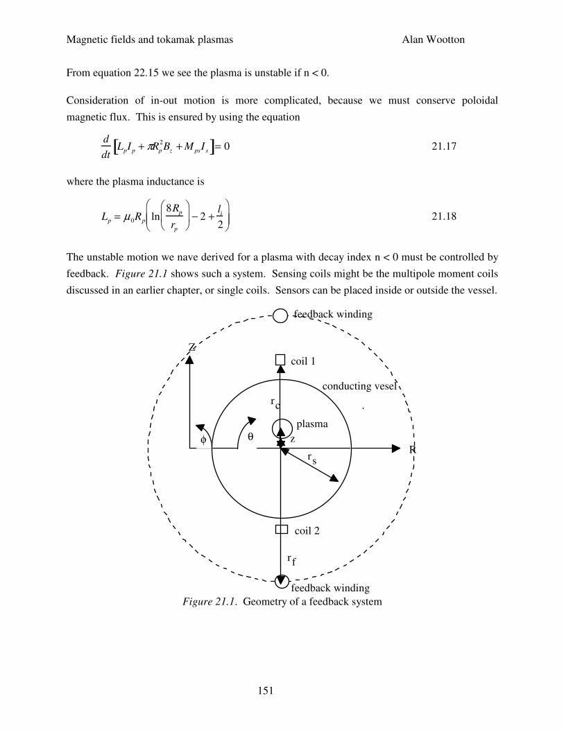
Magnetic fields and tokamak plasmas Alan Wootton
151
From equation 22.15 we see the plasma is unstable if n < 0.
Consideration of in-out motion is more complicated, because we must conserve poloidal
magnetic flux. This is ensured by using the equation
d
dtLpI p + πRp
2Bz + M psI s[ ]= 0 21.17
where the plasma inductance is
Lp = µ0Rp ln8Rp
rp
− 2 +
li
2
21.18
The unstable motion we nave derived for a plasma with decay index n < 0 must be controlled by
feedback. Figure 21.1 shows such a system. Sensing coils might be the multipole moment coils
discussed in an earlier chapter, or single coils. Sensors can be placed inside or outside the vessel.
Z
R
conducting vesel
feedback winding
feedback winding
rf
coil 1
coil 2
z
r
rs
c
φ θplasma
Figure 21.1. Geometry of a feedback system
Magnetic fields and tokamak plasmas Alan Wootton
152
Analysis of sensor coils allowing for vessel currents
If single coils were used, the analysis used to determine plasma displacement z is to take the
difference signal, and divide by the sum signal. For a positive plasma current (into the plane)
and a positive vertical plasma displacement z, the upper coil signal is Bθ1 = µ0Ip/(2π(rc-z)) and
the lower signal is Bθ2 = µ0Ip/(2π(rc+z)), so that for z << rc:
Bθ1 − Bθ 2
Bθ1 + Bθ 2
=
1
rc − z−
1
rc + z
1
rc − z+
1
rc + z
≈z
rc
21.19
We now consider what happens when we allow for the presence of vacuum vessel currents Is and
feedback currents If, both of which produce fields seen by the sensing coils.
The dipole model
The feedback windings are represented by a shell of radius rf and thickness δf with a dipole
current distribution, with current (area) density jφf = jφf0sin(θ). Then
I f = jφf rfδ f dθ = 2rf
0
π
∫ δ f jφf 0 21.20
If is positive when the upper winding current is into the plane. This feedback circuit produces a
major radial field for vertical position control, and (rc < rf):
Bf = K f I f , K f = −µ0
4rf
21.21
That is, a positive If produces a signal Bθ1,f = Bf (which will be negative for positive If) in the
upper sensing coil and a signal Bθ2,f = -Bf (which will be positive for positive If) in the lower
sensing coil.
The vacuum vessel is also assumed to be a shell, of radius rs and thickness δs, carrying a dipole
current jφs = jφs0sin(θ). Then
Is = jφsrsδ sdθ = 2rs
0
π
∫ δ s jφs0 21.22
This produces a major radial field for sensors inside the vessel (rc < rs)
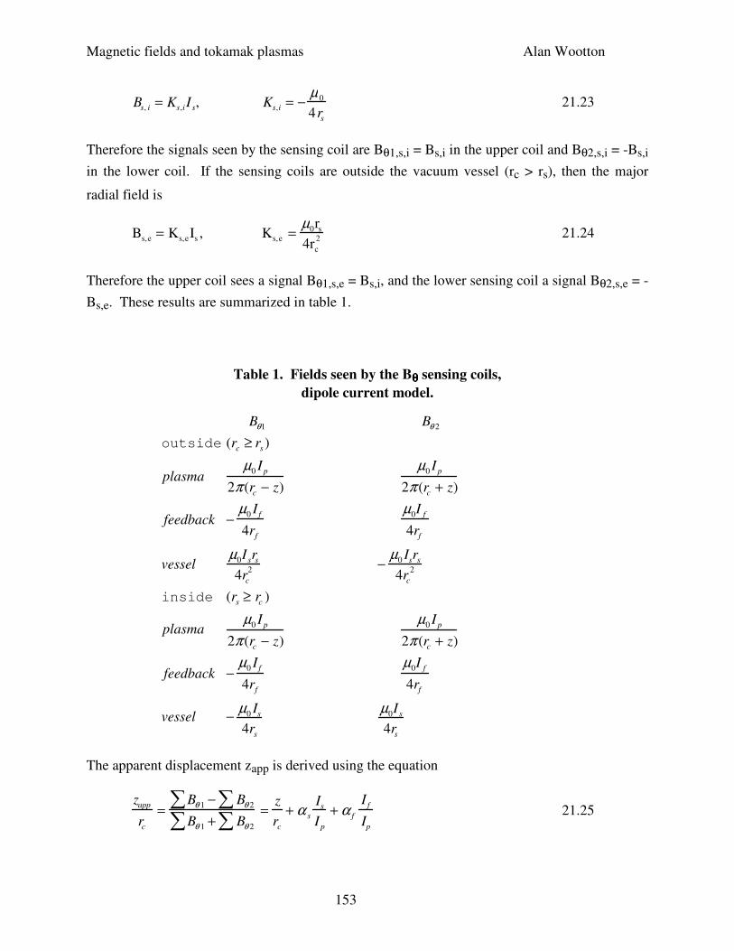
Magnetic fields and tokamak plasmas Alan Wootton
153
Bs, i = Ks,iI s, Ks,i = −µ0
4rs
21.23
Therefore the signals seen by the sensing coil are Bθ1,s,i = Bs,i in the upper coil and Bθ2,s,i = -Bs,i
in the lower coil. If the sensing coils are outside the vacuum vessel (rc > rs), then the major
radial field is
Bs,e = Ks,eIs , Ks,e =µ0rs
4rc
2 21.24
Therefore the upper coil sees a signal Bθ1,s,e = Bs,i, and the lower sensing coil a signal Bθ2,s,e = -
Bs,e. These results are summarized in table 1.
Table 1. Fields seen by the Bθθθθ sensing coils,
dipole current model.
Bθ1 Bθ 2
outside (rc ≥ rs )
plasmaµ0 I p
2π (rc − z)
µ0 I p
2π (rc + z)
feedback −µ0 I f
4rf
µ0I f
4rf
vesselµ0I srs
4rc
2 −µ0 Isrs
4rc
2
inside (rs ≥ rc )
plasmaµ0 I p
2π (rc − z)
µ0 I p
2π (rc + z)
feedback −µ0 I f
4rf
µ0I f
4rf
vessel − µ0 Is
4rs
µ0I s
4rs
The apparent displacement zapp is derived using the equation
zapp
rc
=Bθ 1 − Bθ 2∑∑Bθ 1 + Bθ 2∑∑
=z
rc
+ α s
Is
I p
+ α f
I f
Ip
21.25
Magnetic fields and tokamak plasmas Alan Wootton
154
where the values of αs and αf, derived from the expressions in table 1, are given in table 2.
Without the correction factors αs and αf, zapp = z. Moving the sensors from inside to outside
changes the sign of αs. When the plasma (Ip > 0, into plane) moves upwards (z > 0) it will
induce a negative Is. For sensors outside the vessel, the vessel currents then produce an apparent
displacement smaller than the real displacement (i.e the vacuum vessel shields the sensing coils).
For sensors inside the vessel, the apparent displacement is larger than the true displacement. The
feedback windings complicate this simple process. If we wanted to, the effects of the feedback
coupling to the sensors (i.e. finite αf) can be removed by adding to each signal a term
proportional to If itself. This cannot be done for the coupling from the vessel to the sensors,
because we do not measure the vessel dipole currents.
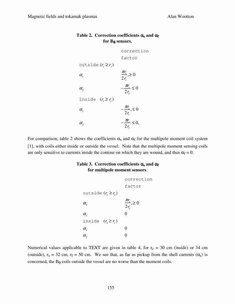
Magnetic fields and tokamak plasmas Alan Wootton
155
Table 2. Correction coefficients ααααs and ααααf
for Bθθθθ sensors.
correction
factor
outside (rc ≥ rs )
αs
πrs
2rc
,≥ 0
α f −πrc
2rf
≤ 0
inside (rs ≥ rc )
αs − πrs
2rc
,≤ 0
α f −πrc
2rf
≤ 0,
For comparison, table 2 shows the coefficients αs and αf for the multipole moment coil system
[1], with coils either inside or outside the vessel. Note that the multipole moment sensing coils
are only sensitive to currents inside the contour on which they are wound, and thus αf = 0.
Table 3. Correction coefficients ααααs and ααααf
for multipole moment sensors.
correction
factor
outside (rc ≥ rs )
αs
πrs
2rc
,≥ 0
α f 0
inside (rs ≥ rc )
αs 0
α f 0
Numerical values applicable to TEXT are given in table 4, for rc = 30 cm (inside) or 34 cm
(outside), rs = 32 cm, rf = 50 cm. We see that, as far as pickup from the shell currents (αs) is
concerned, the Bθ coils outside the vessel are no worse than the moment coils.
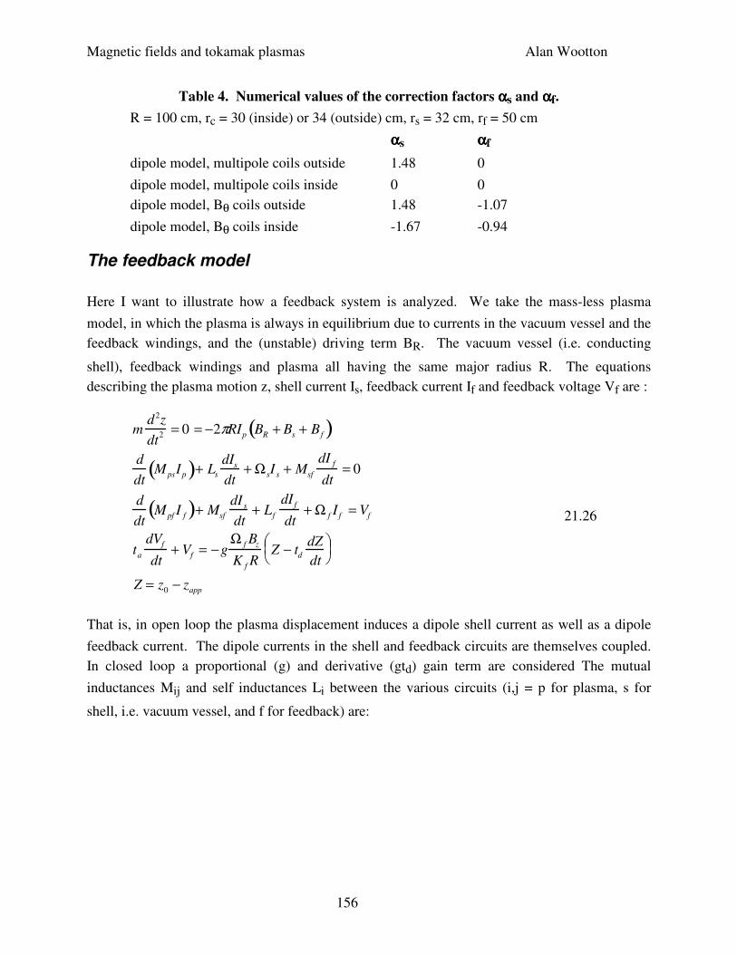
Magnetic fields and tokamak plasmas Alan Wootton
156
Table 4. Numerical values of the correction factors ααααs and ααααf.
R = 100 cm, rc = 30 (inside) or 34 (outside) cm, rs = 32 cm, rf = 50 cm
ααααs ααααf
dipole model, multipole coils outside 1.48 0
dipole model, multipole coils inside 0 0
dipole model, Bθ coils outside 1.48 -1.07
dipole model, Bθ coils inside -1.67 -0.94
The feedback model
Here I want to illustrate how a feedback system is analyzed. We take the mass-less plasma
model, in which the plasma is always in equilibrium due to currents in the vacuum vessel and the
feedback windings, and the (unstable) driving term BR. The vacuum vessel (i.e. conducting
shell), feedback windings and plasma all having the same major radius R. The equations
describing the plasma motion z, shell current Is, feedback current If and feedback voltage Vf are :
md2z
dt2 = 0 = −2πRIp BR + Bs + B f( )
d
dtMpsIp( )+ Ls
dIs
dt+ ΩsI s + Msf
dI f
dt= 0
d
dtMpf I f( )+ Msf
dI s
dt+ Lf
dI f
dt+ Ω f I f = Vf
ta
dVf
dt+ Vf = −g
Ω f Bz
K f RZ − td
dZ
dt
Z = z0 − zapp
21.26
That is, in open loop the plasma displacement induces a dipole shell current as well as a dipole
feedback current. The dipole currents in the shell and feedback circuits are themselves coupled.
In closed loop a proportional (g) and derivative (gtd) gain term are considered The mutual
inductances Mij and self inductances Li between the various circuits (i,j = p for plasma, s for
shell, i.e. vacuum vessel, and f for feedback) are:
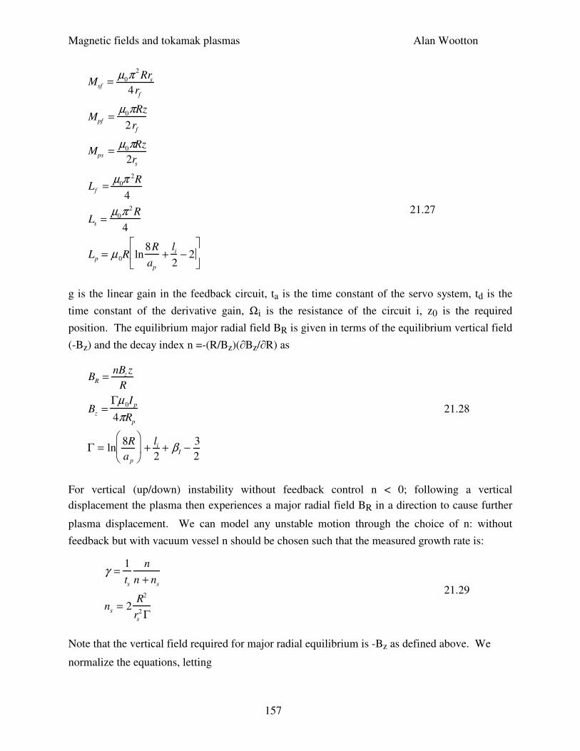
Magnetic fields and tokamak plasmas Alan Wootton
157
Msf = µ0π2Rrs
4rf
Mpf =µ0πRz
2rf
Mps = µ0πRz
2rs
Lf =µ0π
2R
4
Ls =µ0π
2 R
4
Lp = µ 0R ln8R
ap
+li
2− 2
21.27
g is the linear gain in the feedback circuit, ta is the time constant of the servo system, td is the
time constant of the derivative gain, Ωi is the resistance of the circuit i, z0 is the required
position. The equilibrium major radial field BR is given in terms of the equilibrium vertical field
(-Bz) and the decay index n =-(R/Bz)(∂Bz/∂R) as
BR =nBz z
R
Bz =Γµ 0I p
4πRp
Γ = ln8R
a p
+
li
2+ βI − 3
2
21.28
For vertical (up/down) instability without feedback control n < 0; following a vertical
displacement the plasma then experiences a major radial field BR in a direction to cause further
plasma displacement. We can model any unstable motion through the choice of n: without
feedback but with vacuum vessel n should be chosen such that the measured growth rate is:
γ =1
ts
n
n + ns
ns = 2R2
rs
2 Γ
21.29
Note that the vertical field required for major radial equilibrium is -Bz as defined above. We
normalize the equations, letting
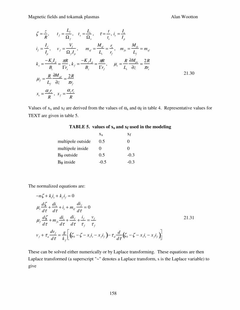
Magnetic fields and tokamak plasmas Alan Wootton
158
ζ = z
R, t f =
Lf
Ω f
, ts = Ls
Ω s
, τ = t
ts
, is = Is
I p
i f =I f
Ip
, v f =Vf
Ω f I p
, msf =Msf
Ls
=rs
rf
, m fs =M fs
Lf
= msf
ks =−Ks I p
Bz
=πR
Γrs
, k f =−K f I p
Bz
=πR
Γrf
, µs =R
Ls
∂Mps
∂z=
2R
πrs
µ f =R
Lf
∂Mpf
∂z=
2R
πrf
xs =α src
R, x f =
α f rc
R
21.30
Values of xs and xf are derived from the values of αs and αf in table 4. Representative values for
TEXT are given in table 5.
TABLE 5. values of xs and xf used in the modeling
xs xf
multipole outside 0.5 0
multipole inside 0 0
Bθ outside 0.5 -0.3
Bθ inside -0.5 -0.3
The normalized equations are:
−nζ + ksis + k f i f = 0
µs
dζdτ
+dis
dτ+ is + msf
di f
dτ= 0
µ f
dζdτ
+ m fs
dis
dτ+
di f
dτ+
i f
τ f
=v f
τ f
v f + τ a
dv f
dτ=
g
k f
ζ0 −ζ − xsis − x f i f( )−τ d
d
dτζ0 −ζ − xsis − x f i f( )
21.31
These can be solved either numerically or by Laplace transforming. These equations are then
Laplace transformed (a superscript "~" denotes a Laplace transform, s is the Laplace variable) to
give
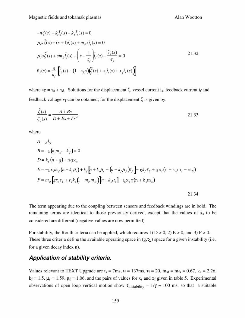
Magnetic fields and tokamak plasmas Alan Wootton
159
−n ˜ ζ (s) + ks˜ i s (s) + k f
˜ i f (s) = 0
µss˜ ζ (s) + (s +1)˜ i s (s) + msf s˜ i f (s) = 0
µ f s˜ ζ (s) + sm fs
˜ i s (s) + s +1
τ f
i f (s) −
˜ v f (s)
τ f
= 0
˜ v f (s) =g
k f
˜ ζ 0 (s) − 1− τΣs( ) ˜ ζ (s) + xs˜ i s (s) + x f
˜ i f (s)( )[ ]
21.32
where τΣ = τa + τd. Solutions for the displacement ζ, vessel current is, feedback current if and
feedback voltage vf can be obtained; for the displacement ζ is given by:
˜ ζ (s)
˜ ζ 0 (s)=
A + Bs
D + Es + Fs2 21.33
where
A = gk f
B = −g ksmsf − k f( )= 0
D = k f n + g( )+ ngxf
E = −gxsmsf n + ks µs( ) + k f n + ksµs + n + k f µ f( )τ f[ ]− gk fτ Σ + gxfn + k
sm
s− ntS( )
F = msf gxsτ Σ +τ fks 1− msf m fs( )[ ]n + ksµ s[ ]− tSxfg n + ksm
s( )
21.34
The term appearing due to the coupling between sensors and feedback windings are in bold. The
remaining terms are identical to those previously derived, except that the values of xs to be
considered are different (negative values are now permitted).
For stability, the Routh criteria can be applied, which requires 1) D > 0, 2) E > 0, and 3) F > 0.
These three criteria define the available operating space in (g,τΣ) space for a given instability (i.e.
for a given decay index n).
Application of stability criteria.
Values relevant to TEXT Upgrade are ts = 7ms, tf = 137ms, τf = 20, msf = mfs = 0.67, ks = 2.26,
kf = 1.5, µs = 1.59, µf = 1.06, and the pairs of values for xs and xf given in table 5. Experimental
observations of open loop vertical motion show τinstability = 1/γ ~ 100 ms, so that a suitable
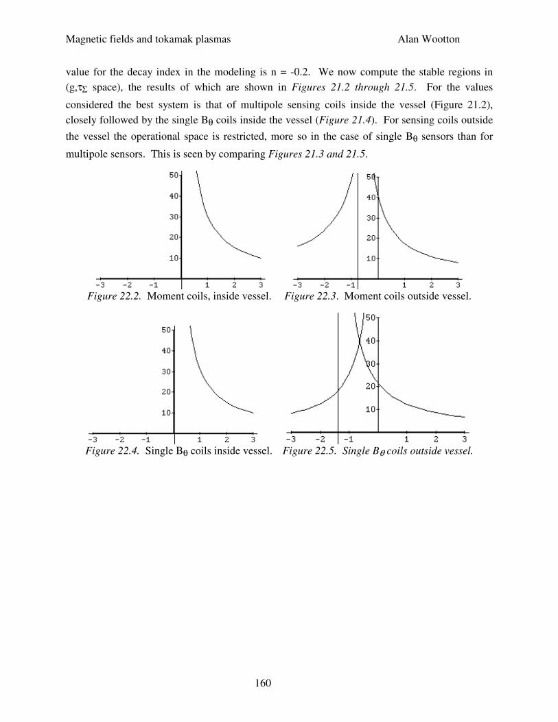
Magnetic fields and tokamak plasmas Alan Wootton
160
value for the decay index in the modeling is n = -0.2. We now compute the stable regions in
(g,τΣ space), the results of which are shown in Figures 21.2 through 21.5. For the values
considered the best system is that of multipole sensing coils inside the vessel (Figure 21.2),
closely followed by the single Bθ coils inside the vessel (Figure 21.4). For sensing coils outside
the vessel the operational space is restricted, more so in the case of single Bθ sensors than for
multipole sensors. This is seen by comparing Figures 21.3 and 21.5.
Figure 22.2. Moment coils, inside vessel. Figure 22.3. Moment coils outside vessel.
Figure 22.4. Single Bθ coils inside vessel. Figure 22.5. Single Bθ coils outside vessel.
Magnetic fields and tokamak plasmas Alan Wootton
161
22. MAGNETIC ISLANDS
We consider the effect of a helical perturbation on a tokamak equilibrium. We will not consider
anything other than vacuum fields, i.e. we will not allow the plasma to respond to the applied
fields in any way. I have adapted the work of S. Matsuda and M. Yoshikawa, in Japanese
Journal of Applied Phys. 14 (1975) 87.
The field line equation is
dl
B= const. 22.1
i.e. working in a quasi cylindrical system based on the plasma center
dθdφ
=R
r
Bθ
Bφ
=1
q(r)= ι(r) 22.2
q is the safety factor, ι the rotational transform. Expanding ι(r) near r = r0, the radius of the
resonant surface, we obtain
dθdφ
≈ ι(r0 ) +dι(r)
drr − r0( ) = ι0 + ι'
x 22.3
where x = r - r0, i0 = i (r0), and ι ' =dι(r)
dr r =r0
. To lowest order in the perturbing field we also
have
dr
rdθ=
dx
rdθ=
br (r,θ,φ)
Bθ (r) 22.4
where br(r,θ,φ) is the radial component of the error field. We ignore the θ component because it
is small compared to the equilibrium field Bθ. Assuming small islands, we also ignore any radial
dependencies of br and Bθ. br is expanded as a Fourier series
br (r0 ,θ,φ) =am,n sin(mθ − nφ) + a
'm ,n sin(mθ + nφ)
+cm, n cos(mθ − nφ) + c 'm ,n cos(mθ + nφ)
m ,n
∑ 22.5
Because we shall see that only resonant components matter near r = r0, we keep only the first and
third terms which satisfy
Magnetic fields and tokamak plasmas Alan Wootton
162
m
n≈
1
ι0
= q0 22.6
Then
br r0 ,θ,φ( )= bm,n sin mθ − nφ + β( ) 22.7
with bm,n = am, n
2 + cm, n
2 and tan β( ) =
bm ,n
am,n
Next we define a new variable
η = mθ − nφ + β 22.8
so that equation 22.4 becomes
dx
r0dθ=
bm ,n sin η( )Bθ (r0 )
22.9
We also obtain from equations 22.3 and 22.8
dηdθ
= −n
ι0 + ι'x
+ m 22.10
Substituting equation 22.9 into equation 2.10 gives us a non linear equation
d2ηdθ 2 = −n
d
dθ1
ι0
1−ι '
ι0
x
= n
r0ι'
ι0
2
bm,n sin η( )Bθ r0( )
= −Asin η( ) 22.11
where
A = −nr0ι
'
ι0
2
bm ,n
Bθ r0( ) 22.12
We can take A > 0 for convenience. We see the behavior of the field lines is analogous to the
motion of a particle in a periodic potential U = A (1-cos(η)), when we regard η and θ as position
and time. Multiplying equation 22.11 by dη/dθ and integrating over θ gives
1
2
dηdθ
2
= E − A(1 − cos η( )) 22.13
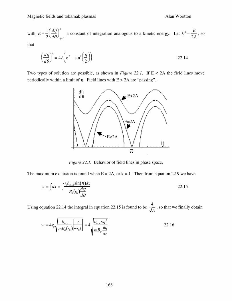
Magnetic fields and tokamak plasmas Alan Wootton
163
with E =1
2
dηdθ
η= 0
2
a constant of integration analogous to a kinetic energy. Let k2 =
E
2A, so
that
dηdθ
2
= 4A k2 − sin
2 η2
22.14
Two types of solution are possible, as shown in Figure 22.1. If E < 2A the field lines move
periodically within a limit of η. Field lines with E > 2A are “passing”.
η
dηθd
E=2A
E>2A
E<2A
η
ηπ
_
Figure 22.1. Behavior of field lines in phase space.
The maximum excursion is found when E = 2A, or k = 1. Then from equation 22.9 we have
w = dx∫ =r0bm, n sin η( )dx
Bθ r0( )dηdθ
∫ 22.15
Using equation 22.14 the integral in equation 22.15 is found to be 4
A, so that we finally obtain
w = 4r0
bm,n
mBθ r0( )ι
−r0ι' = 4
bm ,nr0q2
mBφdq
dr
22.16
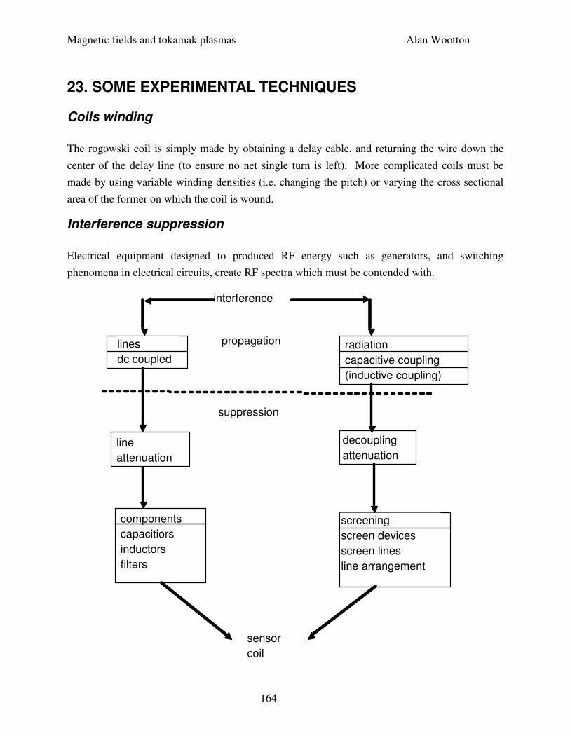
Magnetic fields and tokamak plasmas Alan Wootton
164
23. SOME EXPERIMENTAL TECHNIQUES
Coils winding
The rogowski coil is simply made by obtaining a delay cable, and returning the wire down the
center of the delay line (to ensure no net single turn is left). More complicated coils must be
made by using variable winding densities (i.e. changing the pitch) or varying the cross sectional
area of the former on which the coil is wound.
Interference suppression
Electrical equipment designed to produced RF energy such as generators, and switching
phenomena in electrical circuits, create RF spectra which must be contended with.
interference
propagationlines
dc coupled
radiation
capacitive coupling
(inductive coupling)
suppression
line
attenuation
components
capacitiors
inductors
filters
decoupling
attenuation
screening
screen devices
screen lines
line arrangement
sensor
coil
Magnetic fields and tokamak plasmas Alan Wootton
165
Figure 23.1. An illustration of interference paths and suppression techniques.
The sources of interference are illustrated in Figure 23.1. The interference propagates either
down lines (cables) or by direct radiation. If the wavelength is large compared to the dimensions
of the interference source only minor radiation will result, which is mostly found along the lines.
This is the case for frequencies up to 30 MHz. When the dimension of the interference source is
about that of the wavelength the interference energy will travel by radiation. The dominant
frequencies are those where the interference source are l/4 or multiples of it. Favorable radiation
conditions imply reduced line propagation (because of increased line attenuation) . Therefore the
two propagation paths, comprising direct and capacitive or inductive coupling, suggest two
means of suppression, either line attenuation or de-coupling attenuation. Line attenuation is
effected by filters. De-coupling attenuation is effected by the construction of the sensor coil and
the associated connecting lines.
A common problem with probes is capacitive pick-up. To test for this pick up on simple sensor
coils, two identical and adjacent coils can be connected in series. Depending on the orientation,
the signal obtained should be twice that measured with a single coil, or zero. If the coils
connected in opposition do not give a zero signal, then capacitive coupling effects should be
considered as a possible source of error. Capacitive coupling can be over using a grounded
screen or can around the sensor.
Screened rooms
The requirement is to screen a room in which a sensitive measurement is being performed from
external interference, or to accommodate apparatus which radiate interference in a screened room
to keep the surroundings free from interference. The basic method is to use cages of wire mesh,
or metal sheet. Both electric and magnetic field components must be considered. Units used for
effectiveness are the decibel :
s = 20logE, Bnoscreen
E, Bwithscreen
and the Napier
s = lnE, Bnoscreen
E, Bwithscreen
Magnetic fields and tokamak plasmas Alan Wootton
166
The wire mesh works to screen electric fields because the external flux lines mainly end on the
mesh. The effectiveness depends primarily on the size and type of the mesh. Magnetic screening
is effected by induced currents; DC magnetic fields are not screened, and low frequency AC
magnetic fields are only poorly screened by non magnetic materials. With increasing frequency
the magnetic shielding improves and approaches a finite value. Double screens, insulated from
each other except at one point, improve the screening. These rooms work well to 20 MHz.
Above this the screen room size can equal the cage dimension, causing resonances.
Sheet metal rooms have better screening properties than double walled wire mesh, but breathing
is a problem. The screening against electric fields is ideal since no flux can penetrate. The
screening of the magnetic component improves with increasing frequency due to the skin effect.
Honeycomb inserts are also used. The grids are wave guides (with the frequencies considered
below cut-off), the screening effectiveness of which depends on the ratio of depth to width of the
honeycomb up to cm wavelengths. They are used for 100 kHz < f < 1000 MHz.
Misaligned sensor coils
Typical tokamak requirements include the measurement of poloidal fields in the presence of a
much larger toroidal field. A small misalignment of the coil will then introduce unwanted field
components. There are a number of solution to overcoming this problem
a) subtract data obtained with only the (unwanted) field component by energizing only the
offending windings
b) make use of the differential nature of a pick-up coil signal. For example, consider the
toroidal field to be the offending field, so that the pick-up coil measures dB
dt=
dBpoloidal
dt+
dBtoroidal
dt. If the toroidal field is almost steady state (d/dt ≈ 0) during the times of
interest, then the differential signal during this time is approximately that required (i.e. from the
poloidal field component only). Therefore the temporal integration should be started as late as
possible.