The University of Manchester Research

Magnetic Field Frequency Optimisation for MFL Imagingusing QWHE Sensors

Link to publication record in Manchester Research Explorer

Citation for published version (APA):Watson, J. M., Liang, C-W., Sexton, J., & Missous, M. (2019). Magnetic Field Frequency Optimisation for MFLImaging using QWHE Sensors. Paper presented at 58th Annual British Conference on Non-Destructive Testing,Telford, United Kingdom.

Citing this paperPlease note that where the full-text provided on Manchester Research Explorer is the Author Accepted Manuscriptor Proof version this may differ from the final Published version. If citing, it is advised that you check and use thepublisher's definitive version.

General rightsCopyright and moral rights for the publications made accessible in the Research Explorer are retained by theauthors and/or other copyright owners and it is a condition of accessing publications that users recognise andabide by the legal requirements associated with these rights.

Takedown policyIf you believe that this document breaches copyright please refer to the University of Manchester’s TakedownProcedures [http://man.ac.uk/04Y6Bo] or contact uml.scholarlycommunications@manchester.ac.uk providingrelevant details, so we can investigate your claim.

Download date:14. Mar. 2022

Magnetic Field Frequency Optimisation for MFL Imaging using QWHE Sensors

Journal: 58th Annual British Conference on Non-Destructive Testing

Manuscript ID NDT-0028-2019.R1

Topic: Electromagnetics

Date Submitted by the Author: n/a

Complete List of Authors: Watson, James; University of Manchester, School of Electrical and Electronic Engineering

Keywords: Electromagnetics, Magnetic flux leakage, Magnetic particles, Eddy currents, Image formation, Frequencies

Magnetic Field Frequency Optimisation for MFL Imaging using

QWHE Sensors

J. M. Watson, C.W. Liang, J. Sexton and M. Missous

University of Manchester, Department of Electrical and Electronic Engineering

Manchester, M13 9PL, United Kingdom

james.watson-6@postgrad.manchester.ac.uk

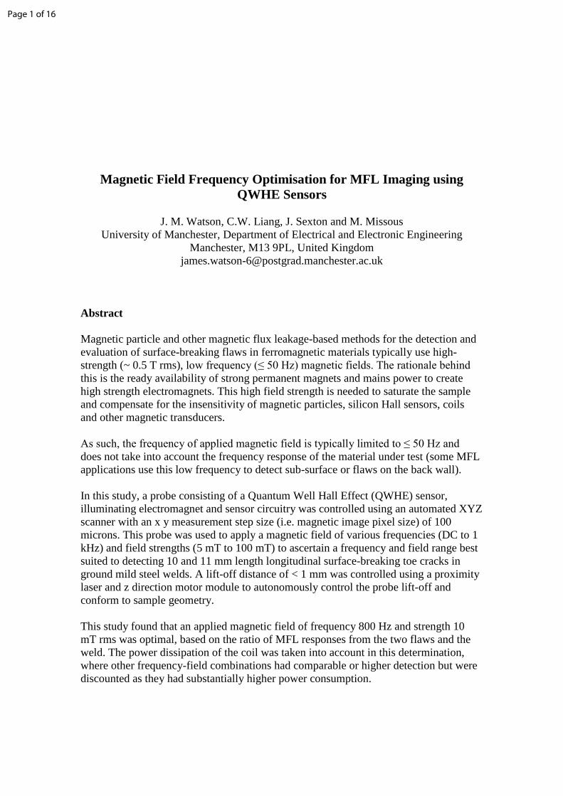
Abstract

Magnetic particle and other magnetic flux leakage-based methods for the detection and

evaluation of surface-breaking flaws in ferromagnetic materials typically use high-

strength (~ 0.5 T rms), low frequency (≤ 50 Hz) magnetic fields. The rationale behind

this is the ready availability of strong permanent magnets and mains power to create

high strength electromagnets. This high field strength is needed to saturate the sample

and compensate for the insensitivity of magnetic particles, silicon Hall sensors, coils

and other magnetic transducers.

As such, the frequency of applied magnetic field is typically limited to ≤ 50 Hz and

does not take into account the frequency response of the material under test (some MFL

applications use this low frequency to detect sub-surface or flaws on the back wall).

In this study, a probe consisting of a Quantum Well Hall Effect (QWHE) sensor,

illuminating electromagnet and sensor circuitry was controlled using an automated XYZ

scanner with an x y measurement step size (i.e. magnetic image pixel size) of 100

microns. This probe was used to apply a magnetic field of various frequencies (DC to 1

kHz) and field strengths (5 mT to 100 mT) to ascertain a frequency and field range best

suited to detecting 10 and 11 mm length longitudinal surface-breaking toe cracks in

ground mild steel welds. A lift-off distance of < 1 mm was controlled using a proximity

laser and z direction motor module to autonomously control the probe lift-off and

conform to sample geometry.

This study found that an applied magnetic field of frequency 800 Hz and strength 10

mT rms was optimal, based on the ratio of MFL responses from the two flaws and the

weld. The power dissipation of the coil was taken into account in this determination,

where other frequency-field combinations had comparable or higher detection but were

discounted as they had substantially higher power consumption.

Page 1 of 16

2

1. Introduction

Complimentary electromagnetic Non Destructive Testing and Evaluation (NDT&E)

techniques are often the preferred choice for surface-breaking flaw detection and

evaluation in mild steels due to the versatility and large inspection area of Magnetic

Particle Inspection (MPI) (1), as well as the depth measurement and higher sensitivity

(due to the electromagnetic skin effect) of conventional Eddy Current Testing (ECT) (2)

and other eddy current-based technologies and methods (3).

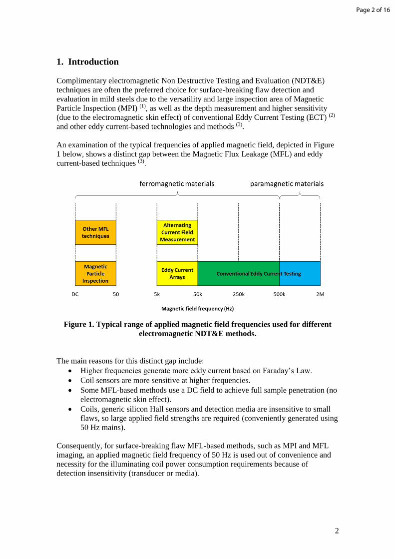
An examination of the typical frequencies of applied magnetic field, depicted in Figure

1 below, shows a distinct gap between the Magnetic Flux Leakage (MFL) and eddy

current-based techniques (3).

Figure 1. Typical range of applied magnetic field frequencies used for different

electromagnetic NDT&E methods.

The main reasons for this distinct gap include:

Higher frequencies generate more eddy current based on Faraday’s Law.

Coil sensors are more sensitive at higher frequencies.

Some MFL-based methods use a DC field to achieve full sample penetration (no

electromagnetic skin effect).

Coils, generic silicon Hall sensors and detection media are insensitive to small

flaws, so large applied field strengths are required (conveniently generated using

50 Hz mains).

Consequently, for surface-breaking flaw MFL-based methods, such as MPI and MFL

imaging, an applied magnetic field frequency of 50 Hz is used out of convenience and

necessity for the illuminating coil power consumption requirements because of

detection insensitivity (transducer or media).

Page 2 of 16

3

As such, typical surface-breaking flaw MFL-based methods are not truly optimised to

the magnetic response of the sample material.

This study involved using Quantum Well Hall Effect (QWHE) sensors developed at The

University of Manchester (4) to ascertain if there was any optimum applied magnetic

field frequency or field strength range for a particular type and size of flaws. The

QWHE sensors were used because of their proven ability to detect the MFL response

from real NDE flaws (5). A previous comparative study (6) (7) suggests they have a

detection performance comparable to conventional ECT. This sensor system technology

has high quality imaging capabilities (8) with better flaw characterisation than eddy

current-based images and has additional weld information (9).

Key attributes of the QWHE sensors include:

Ability to be made into bespoke arrays with specific size (2 µm to 70 µm) and

sensor pitch (< 20 µm).

Sensitive to only one component of the sample magnetic field response, i.e. Bz in

Equation 1.

High sensitivity which is limited by biasing and detection circuit electronics

(currently 20 nT detection limit in both AC and DC using superheterodyne

techniques).

Large dynamic range of 20 nT to ~2 T (160 dB) for versatility with no hysteresis

offset unlike Giant Magnetoresistors (GMRs) and other anisotropic

magnetoresistance-based transducers.

Linear across large dynamic range and wide bandwidth from DC to MHz range.

It is the unique combination of sensitivity and linearity over a large dynamic range that

make QWHE sensors versatile for different NDT&E applications, in particular,

optimised low-power high-quality (flaw characterisation) MFL imaging technology.

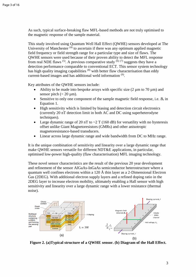
These novel sensor characteristics are the result of the previous 20 year development

and refinement of the sensor AlGaAs-InGaAs semiconductor heterostructure where a

quantum well confines electrons within a 120 Å thin layer as a 2-Dimensional Electron

Gas (2DEG). With additional electron supply layers and a refined doping ratio in the

2DEG layer to increase electron mobility, ultimately enabling a Hall sensor with high

sensitivity and linearity over a large dynamic range with a lower resistance (thermal

noise).

(a)

(b)

Figure 2. (a)Typical structure of a QWHE sensor. (b) Diagram of the Hall Effect.

Page 3 of 16

4

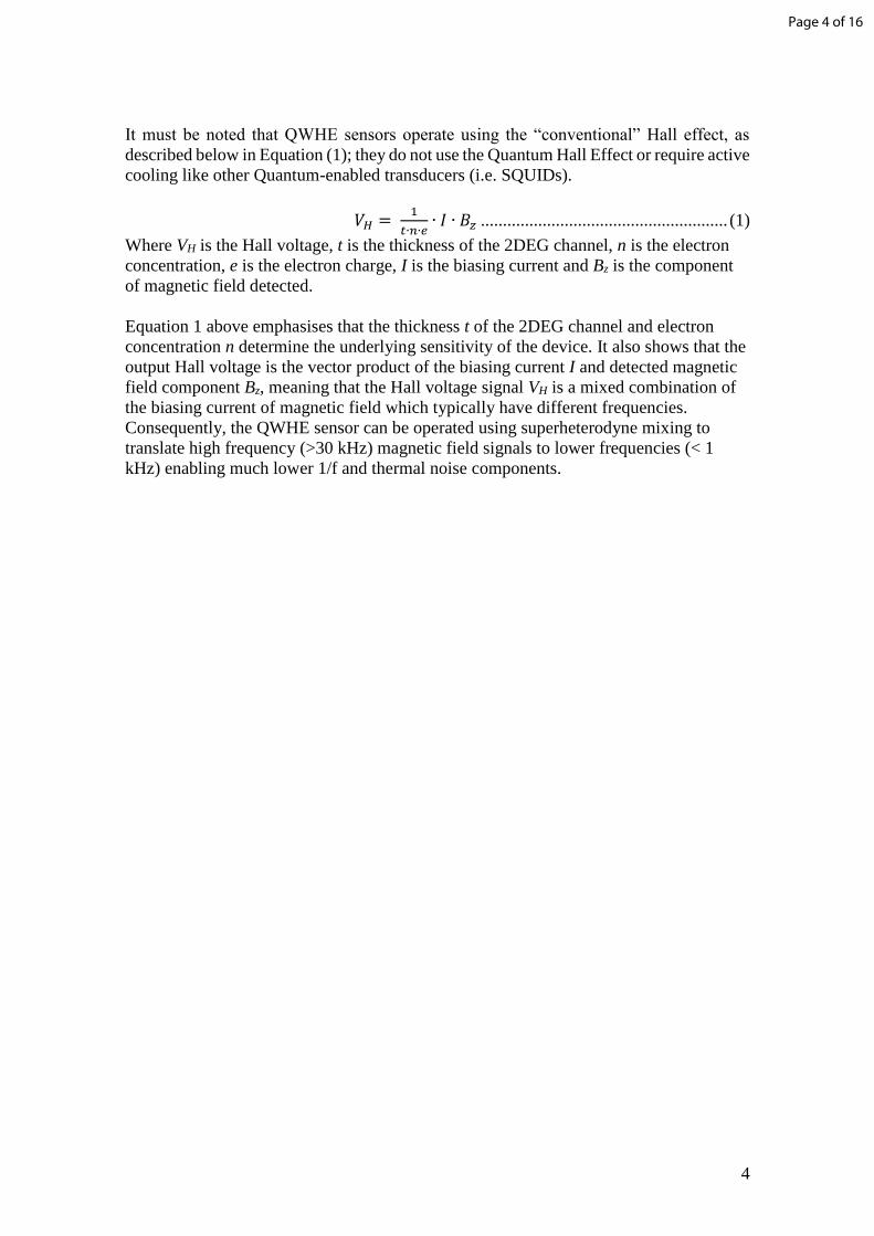
It must be noted that QWHE sensors operate using the “conventional” Hall effect, as

described below in Equation (1); they do not use the Quantum Hall Effect or require active

cooling like other Quantum-enabled transducers (i.e. SQUIDs).

𝑉𝐻 = 1

𝑡∙𝑛∙𝑒∙ 𝐼 ∙ 𝐵𝑧 ........................................................ (1)

Where VH is the Hall voltage, t is the thickness of the 2DEG channel, n is the electron

concentration, e is the electron charge, I is the biasing current and Bz is the component

of magnetic field detected.

Equation 1 above emphasises that the thickness t of the 2DEG channel and electron

concentration n determine the underlying sensitivity of the device. It also shows that the

output Hall voltage is the vector product of the biasing current I and detected magnetic

field component Bz, meaning that the Hall voltage signal VH is a mixed combination of

the biasing current of magnetic field which typically have different frequencies.

Consequently, the QWHE sensor can be operated using superheterodyne mixing to

translate high frequency (>30 kHz) magnetic field signals to lower frequencies (< 1

kHz) enabling much lower 1/f and thermal noise components.

Page 4 of 16

5

2. MFL Imaging using QWHE Sensors

This section provides information on the sample used in this study, as well as an

overview of the QWHE sensor scanner used, the data acquisition steps of the system

and the data collection procedures.

2.1 Sample Under Test

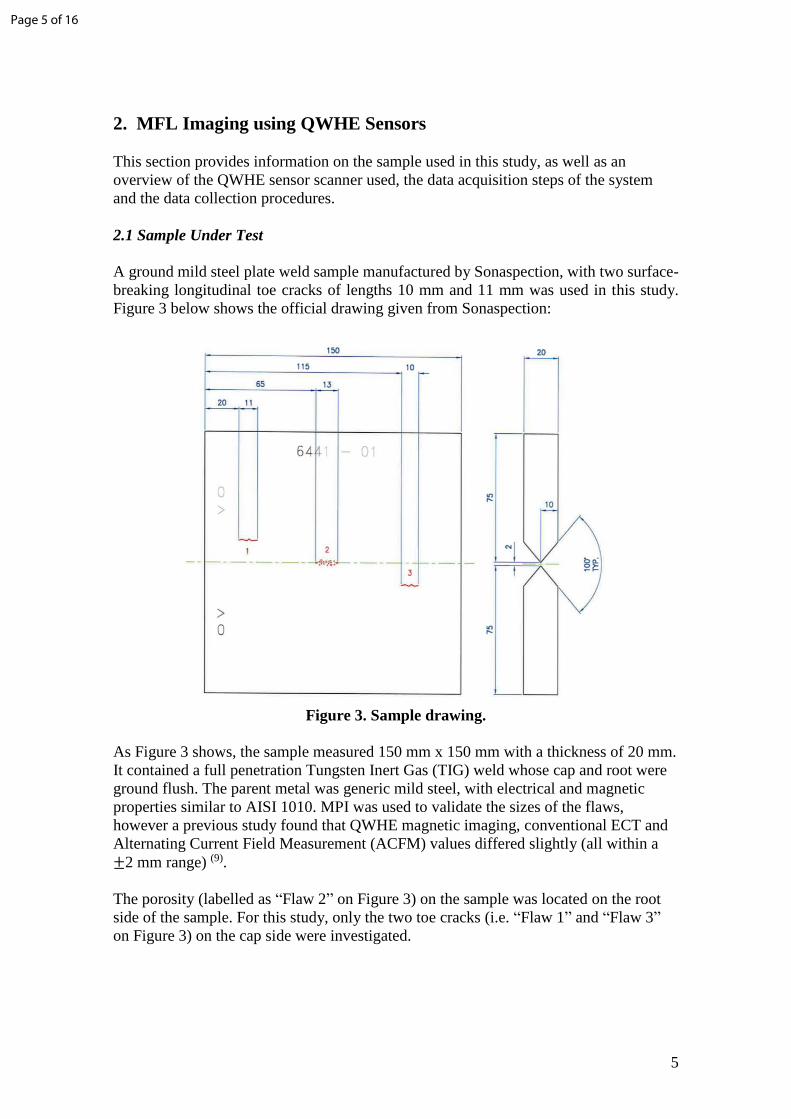
A ground mild steel plate weld sample manufactured by Sonaspection, with two surface-

breaking longitudinal toe cracks of lengths 10 mm and 11 mm was used in this study.

Figure 3 below shows the official drawing given from Sonaspection:

Figure 3. Sample drawing.

As Figure 3 shows, the sample measured 150 mm x 150 mm with a thickness of 20 mm.

It contained a full penetration Tungsten Inert Gas (TIG) weld whose cap and root were

ground flush. The parent metal was generic mild steel, with electrical and magnetic

properties similar to AISI 1010. MPI was used to validate the sizes of the flaws,

however a previous study found that QWHE magnetic imaging, conventional ECT and

Alternating Current Field Measurement (ACFM) values differed slightly (all within a

±2 mm range) (9).

The porosity (labelled as “Flaw 2” on Figure 3) on the sample was located on the root

side of the sample. For this study, only the two toe cracks (i.e. “Flaw 1” and “Flaw 3”

on Figure 3) on the cap side were investigated.

Page 5 of 16

6

2.2 QWHE Imaging XYZ Scanner

The developed scanner (6) (7) autonomously controlled the fine movement of a probe

consisting of a 10 µm size QWHE sensor and its biasing/detection circuitry, along with

an illuminating electromagnet. The electromagnet applied a magnetic field of precisely

known frequency and field strength to the sample, with the QWHE sensor and data

acquisition system mapping the MFL response for each x and y position on the sample

surface.

A proximity laser on the probe was used to take an initial topographical scan of the region

to be magnetically imaged. An additional z direction motor module was used to

autonomously control the probe lift-off, using the laser map to compensate for changes

in lift-off due to sample curvature. This was done to avoid damage to the probe head and

sample, as well as provide better quality magnetic images.

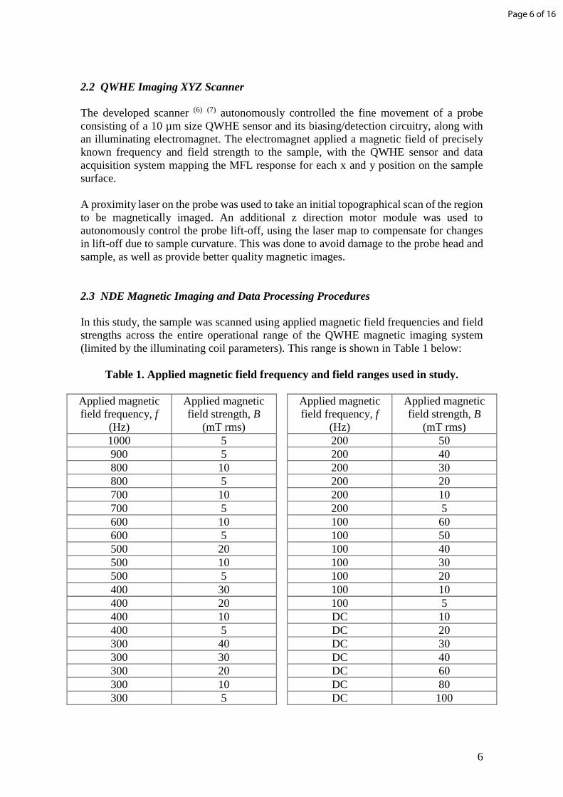
2.3 NDE Magnetic Imaging and Data Processing Procedures

In this study, the sample was scanned using applied magnetic field frequencies and field

strengths across the entire operational range of the QWHE magnetic imaging system

(limited by the illuminating coil parameters). This range is shown in Table 1 below:

Table 1. Applied magnetic field frequency and field ranges used in study.

Applied magnetic

field frequency, f

(Hz)

Applied magnetic

field strength, B

(mT rms)

Applied magnetic

field frequency, f

(Hz)

Applied magnetic

field strength, B

(mT rms)

1000 5 200 50

900 5 200 40

800 10 200 30

800 5 200 20

700 10 200 10

700 5 200 5

600 10 100 60

600 5 100 50

500 20 100 40

500 10 100 30

500 5 100 20

400 30 100 10

400 20 100 5

400 10 DC 10

400 5 DC 20

300 40 DC 30

300 30 DC 40

300 20 DC 60

300 10 DC 80

300 5 DC 100

Page 6 of 16

7

The sample was firmly secured to the scanner bed to ensure no movement during the

scans (particularly at DC where strong field strengths can pick up the sample). A fine

measurement step of 100 µm for x and y was used (giving a pixel size of 100 µm x 100

µm), with a 0.75 mm lift-off to ensure adequate clearance throughout the scanning.

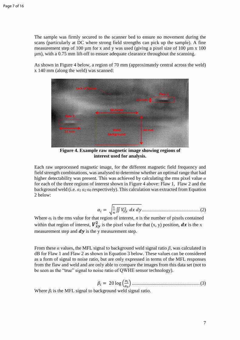
As shown in Figure 4 below, a region of 70 mm (approximately central across the weld)

x 140 mm (along the weld) was scanned:

Figure 4. Example raw magnetic image showing regions of

interest used for analysis.

Each raw unprocessed magnetic image, for the different magnetic field frequency and

field strength combinations, was analysed to determine whether an optimal range that had

higher detectability was present. This was achieved by calculating the rms pixel value α

for each of the three regions of interest shown in Figure 4 above: Flaw 1, Flaw 2 and the

background weld (i.e. α1 α2 α0 respectively). This calculation was extracted from Equation

2 below:

𝛼𝑖 = √1

𝑛∬ 𝑉𝑥𝑦

2 𝑑𝑥 𝑑𝑦 ................................................ (2)

Where αi is the rms value for that region of interest, n is the number of pixels contained

within that region of interest, 𝑽𝒙𝒚𝟐 is the pixel value for that (x, y) position, 𝒅𝒙 is the x

measurement step and 𝒅𝒚 is the y measurement step.

From these α values, the MFL signal to background weld signal ratio β, was calculated in

dB for Flaw 1 and Flaw 2 as shown in Equation 3 below. These values can be considered

as a form of signal to noise ratio, but are only expressed in terms of the MFL responses

from the flaw and weld and are only able to compare the images from this data set (not to

be seen as the “true” signal to noise ratio of QWHE sensor technology).

𝛽𝑖 = 20 log (𝛼𝑖

𝛼0) ........................................................ (3)

Where βi is the MFL signal to background weld signal ratio.

Page 7 of 16

8

In addition, the mean β value, �̅�, for each applied magnetic field frequency and field

strength combination was calculated in dB as show in Equation 4 below:

�̅� = 20 log (𝛼1+𝛼2

2 𝛼0) .................................................... (4)

The 𝛽1, 𝛽2 and �̅� values for each applied magnetic field frequency and field strength

combination were then plotted against applied magnetic field frequency and field strength

to ascertain any optimum range. These plots are shown and discussed in the results

section.

Figure 4 shows that the full width of the weld in the sample was not used in the

calculations because of a suspected lack of fusion. Although the sample was validated for

general magnetic testing, the previous comparative study found that ECT and ACFM also

detected this feature. As such, the presence of this within the weld background signal α0

would make it not representative of a “clean” weld and would have greatly influenced the

outcomes and therefore it was excluded from the calculations.

All of the scans were performed consecutively to minimise any environmental changes

(different lift-off, condition of the system, magnetisation of the sample from a different

measurement, etc.) that could have affected the results. In addition, the DC scans were

performed at the end in ascending order to prevent a previous higher strength scan

affecting the measurement via residual magnetisation of the coil core or sample.

Page 8 of 16

9

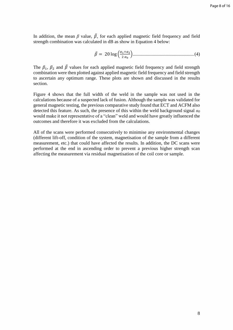
3. Results and Discussion

This study produced 40 QWHE magnetic images from the different applied magnetic

field frequency and field strength combinations across the operational range of the XYZ

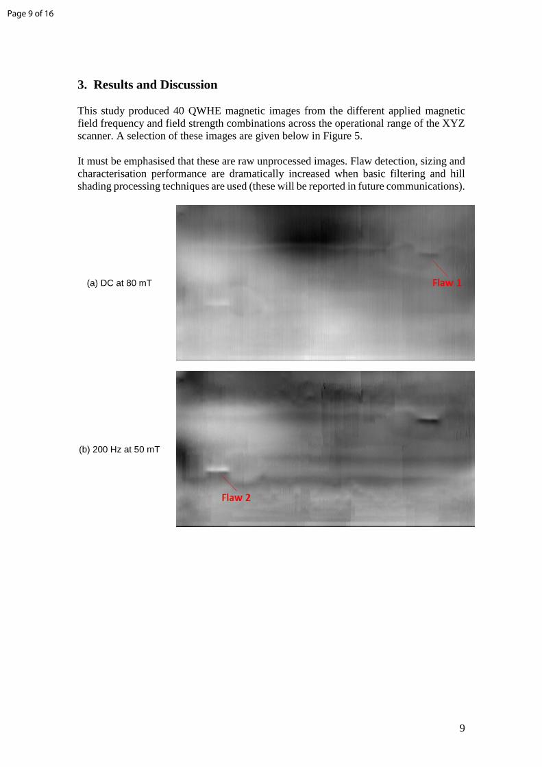
scanner. A selection of these images are given below in Figure 5.

It must be emphasised that these are raw unprocessed images. Flaw detection, sizing and

characterisation performance are dramatically increased when basic filtering and hill

shading processing techniques are used (these will be reported in future communications).

(a) DC at 80 mT

(b) 200 Hz at 50 mT

Page 9 of 16

10

(d) 600 Hz at 10 mT

(f) 1000 Hz at 5 mT

Figure 5. Selection of QWHE magnetic images at different applied magnetic

field frequencies and field strengths. Annotated to show weld features.

For each of these 40 magnetic images, the MFL signal to background weld signal ratio β

for each flaw was calculated, along with the �̅� value for each image. These are plotted in

Figure 6 below:

Page 10 of 16

11

(a) Flaw 1

0 200 400 600 800 1000

-2

-1

0

1

2

3

4

5

MF

L S

igna

l to

Ba

ckgro

und

We

ld

Sig

na

l R

atio

1 (

dB

)

Applied Magnetic Field Frequency (Hz)

5 mT

10 mT

20 mT

30 mT

40 mT

50 mT

60 mT

80 mT

100 mT

(b) Flaw 2

0 200 400 600 800 1000

-2

0

2

4

6

8

MF

L S

ignal to

Backgro

und W

eld

Sig

nal R

atio

2 (

dB

)

Applied Magnetic Field Frequency (Hz)

5 mT

10 mT

20 mT

30 mT

40 mT

50 mT

60 mT

80 mT

100 mT

(c) Mean

0 200 400 600 800 1000

-2

-1

0

1

2

3

4

5

Mea

n M

FL

Sig

na

l to

Ba

ckgro

und

We

ld S

igna

l R

atio

(

dB

)

Applied Magnetic Field Frequency (Hz)

5 mT

10 mT

20 mT

30 mT

40 mT

50 mT

60 mT

80 mT

100 mT

Figure 6. Plots of β1, β2 and �̅� for the various applied magnetic field

frequency and field strength combinations.

Page 11 of 16

12

From Figure 6 above it is clear that, in general, the β2 values were higher than β1, which

can also be seen in the images shown in Figure 5 where Flaw 2 appears whiter than Flaw

1. Also, it must be emphasised that the β values do not portray the “true” signal to noise

ratio of the QWHE XYZ scanner or the MFL technique in general, since they could be

dramatically increased by reducing the region of interest of Flaw 1 and Flaw 2, giving

higher α and therefore higher β values too. As such, β values are used only to

quantitatively compare the 40 images within this study data set.

Figure 6c also shows two particular applied magnetic field frequency and field strength

regions of interest: 300 to 400 Hz at 40 and 30 mT respectively, as well as 800 Hz at 10

mT. Based on these, the power dissipations, Wcoil, for each applied magnetic field

frequency and field strength combination were calculated using initial control calibrations

of the XYZ scanning system. This was deemed important in establishing if an optimum

frequency-field range exists, since although the �̅� values for 300 Hz 40 mT and 400 Hz

30 mT were higher than those of 800 Hz 10 mT, they required a much higher power to

achieve this.

The power dissipation in the coil (Wcoil) values were then plotted along with the other

inspection parameters including applied magnetic field strength, �̅� and applied magnetic

field frequency as shown in Figure 7 below:

Figure 7. Plot of �̅� values against applied magnetic field frequency and field

strength, as well as power dissipation of the coil.

Figure 7 above clearly shows a general trend where the low power, low strength applied

magnetic fields have a substantially low �̅�. This also includes the higher frequency

outlier

Page 12 of 16

13

combinations where only low strength fields can be applied due to the larger coil

impedance.

More importantly, Figure 7 suggests that the outlier of applying 800 Hz at 10 mT is

optimal, based on the comparatively higher β from both flaws, along with considerably

lower (< 35%) power consumption requirements of applied magnetic field frequency and

field strength combinations with comparable or higher �̅� values. Although it is out of the

scope of this work to prove any explanation of the study findings, some conjectures are

discussed next.

Using electrical conductivity and magnetic permeability values of AISI 1010, the skin

depths at 800 Hz, 900 Hz and 1000 Hz are approximately 210 µm 200 µm and 190 µm

respectively. The differences between these are negligible. Therefore, it can be suggested

that the 800 Hz 10 mT has effectively double the magnetic field strength confined (since

the field strengths were 5 mT for both the 900 Hz and 1000 Hz frequencies), producing

more leakage near the flaw-sample boundaries. Therefore, it can be argued that the

illumining coil parameters of the QWHE XYZ scanner are potentially biased/optimised

to 800 Hz: in this instance being the only low power, high frequency, higher-strength (>

5 mT) applied field combination possible with the illuminating coil parameters. In which

case, the optimisation is not an underlying MFL principle; and that different illuminating

coil parameters may respond with a different optimal frequency-field range. However,

the �̅� values for 600 Hz and 700 Hz at 10 mT are significantly lower than 800 Hz, despite

having approximate skin depths of 245 µm and 225 µm respectively, being not too

dissimilar to 800 Hz.

It can be argued that since this 800 Hz 10 mT combination is the only low power, high

frequency, higher-strength applied field combination, under these conditions the flaws

will be subjected to more eddy currents and hence a better detectability. However, it must

be emphasised that the footprint of the applied magnetic field is extremely localised: 5

mm x 15 mm, and is orientated perpendicular to the major axis of the flaws.

Consequently, the eddy currents produced will not be disrupted by the flaws as they will

be orientated parallel to the flaws, flowing in the z-y plane shown in Figure 2. The eddy

current secondary magnetic fields, although orientated perpendicular to the flaw, will also

not produce an MFL response since they will be in the opposing direction of the applied

magnetic field.

Alternatively, it can be also speculated that at 800 Hz the magnetic permeability

differences between the parent steel plates, the weld metal and microstructures in the heat

affected zone are dramatically reduced. This in turn leads to much lower MFL responses

from the weld and other contributors of the background weld signal, giving higher �̅�

values. This proposal also explains why the 600 Hz and 700 Hz 10 mT measurements had

significantly lower �̅� values despite also having similar skin depths (not considered too

different to warrant the 3 to 2 dB differences respectively). Figure 6 also suggests 600 Hz

as an inflexion point, where the �̅� values for the same strength applied magnetic field start

to increase dramatically with frequency after this point.

Page 13 of 16

14

It must be noted that although these measurements and analysis suggest an optimum

frequency and field strength range, this is only applicable to the measurement set up used,

along with numerous other inspection parameters including:

Flaw type.

Flaw size and depth.

Sample material electrical and magnetic properties.

Surface finish of sample.

Illuminating coil parameters (number of turns, core material, driver current, etc.).

Applied magnetic field footprint.

Lift-off distance.

Repeating this study and adding new data points to Figure 6, as well as being able to

determine the variance between �̅� values of the same applied magnetic field frequency

and field strength values, would add more confidence to the investigations carried out

here. In addition, it would be of interest to repeat the study using a different length toe

crack and different illuminating coil parameters to observe any effect that these would

have on an optimum applied magnetic field frequency and field strength range.

Furthermore, it would also be of interest to repeat the study using different electromagnet

parameters to better suit > 5 mT fields at > 1 kHz, namely decreasing the number of turns

and using a core material with less hysteresis loss (such as composite or ferrite) to test

some of the conjectures put forward to explain the results of the study.

Page 14 of 16

15

4. Conclusions

In this work, 40 magnetic images using a QWHE sensor XYZ scanner were obtained with

various applied magnetic field frequency and field strengths across the complete

operational range of the scanner.

Quantitative analysis was then performed to determine that an applied magnetic field

frequency of 800 Hz of 10 mT rms strength was optimal for the detection of the 11 mm

and 10 mm length surface-breaking toe cracks in a ground mild steel weld sample. This

applied magnetic field frequency and field strength pair was the result of the combination

of comparatively high detectability and low power consumption of the illuminating coil.

Future work being undertaken to develop the maturity of the QWHE imaging technique

includes:

Repeating the study, using smaller length toe cracks in the same sample material to

ascertain the effect of flaw size on the optimum frequency.

Repeating the study, using a much larger applied magnetic field footprint to

ascertain the effect of footprint on the optimum frequency.

Repeating the study, using various lift-off values to measure the effect of lift-off for

MFL imaging using QWHE sensors.

Processing the dataset from this study to determine a minimum / optimum

measurement step where the flaws are still detectable (for optimum sensor array

pitch).

Developing enhanced, optimised imaging technology based on this underpinning

research.

Developing image enhancement techniques and automated flaw detection and

sizing algorithms using frequency-based analysis and/or spatial MFL field

distribution around flaws.

Building a database of MFL responses from flaws of known dimensions for future

enhanced characterisation and reconstruction.

Developing multi-frequency / pulsed applied magnetic field technologies for

detection, imaging, sizing and characterisation of surface-breaking and near-

surface flaws (< 3 mm from surface).

Acknowledgements

EPSRC-EP/P006973/1 “FUTURE COMPOUND SEMI-CONDUCTOR

MANUFACTURING HUB”)

EPSRC-EP/LO22125/1 “UK RESEARCH CENTRE IN NON-DESTRUCTIVE

EVALUATION(RCNDE3)”

ICASE PhD STUDENTSHIP THROUGH RCNDE (BAE Systems)

Page 15 of 16

16

References

1. British Standard BS EN ISO 9934-1:2016. Non-destructive testing – Magnetic

particle testing. Part 1: General principles (ISO 9934-1:2016), 2016.

2. British Standard BS EN ISO 15549:2010. Non-destructive testing – Eddy current

testing – General principles, 2010.

3. S. S. Udpa, ‘NDT Handbook – Electromagnetic Testing’ (3rd ed.). Columbus:

American Society for Nondestructive Testing, 2004.

4. N. Haned and M. Missous, ‘Nano-tesla magnetic field magnetometry using an

InGaAs-AlGaAs-GaAs 2DEG Hall sensor’, Sensors and Actuators, 102(3), 216-

222. DOI 10.1016/S0924-4247(02)00386-2, 2003.

5. J. M. Watson, C.W. Liang, E. Ahmad, J. Sexton and M. Missous, ‘Surface Crack

Detection in Dressed Steel Welds Using Advanced Quantum Well Hall Effect

Sensors’, 56th Annual Conference of the British Institute of Non-Destructive

Testing, 2017.

6. J. M. Watson, C.W. Liang, J. Sexton, F. A. Biruu and M. Missous, ‘A Comparative

Study of Electromagnetic NDE Methods and Quantum Well Hall Effect Sensor

Imaging for Surface-Flaw Detection in Mild Steel Welds’, 57th Annual British

Conference on Non-Destructive Testing, 2018.

7. J. M. Watson, C.W. Liang, J. Sexton, F. A. Biruu and M. Missous, ‘Surface-

Breaking Flaw Detection in Ferritic Welds using Quantum Well Hall Effect Sensor

Devices’, 45th Annual Review of Progress in Quantitative Nondestructive

Evaluation, 2018.

8. C. W. Liang, E. Ahmad, E. Balaban, F. A. Biruu, J. Sexton and M. Missous, ‘A Real

Time Quantum Well Hall Effect 2D Handheld Magnetovision System for

Ferromagnetic and Non-Ferromagnetic Materials Nondestructive Testing’, 56th

Annual Conference of the British Institute of Non-Destructive Testing, 2017.

9. E. Ahmad, J. Watson, C. W. Liang, J. Sexton and M. Missous, ‘RCNDE Core

Research Review Report: July 2018. Sub-Project 1.3: Magnetic Camera’, RCNDE

Board, 2018.

Page 16 of 16