Page 1/15

Magnetic and Soil Parameters as a Potential Indicator of Soil PollutionMohammed Murthuza  ( muthuza2021@gmail.com )

Government Arts CollegeSurumbar Kuzhali 

Government Arts CollegeLakshmi Narasimhan 

Anna University Chennai.Thirukumaran V 

Government Arts CollegeChandrasekaran A 

SSN College of Engineering: Sri Sivasubramaniya Nadar College of EngineeringDurai Ganesh 

Government Arts CollegeRavi sankar 

Government Arts College

Research Article

Keywords: Soil, physico-chemical properties, magnetic susceptibility, Statistical Methods, Pollution

Posted Date: June 17th, 2021

DOI: https://doi.org/10.21203/rs.3.rs-497474/v1

License: This work is licensed under a Creative Commons Attribution 4.0 International License.   Read Full License

Page 2/15

AbstractThe aim of this study was to look into the effect of land use or human activity on soil samples and to distinguish between pollution from anthropogenicsources or natural sources using magnetic susceptibility and statistical method. In soil samples from Tiruvannamalai Dist, Tamilnadu, magnetic susceptibilitymeasurements at low frequency (lf) and high frequency (hf) were carried out. The physic-chemical properties such as % of sand, silt, clay, Electricalconductivity (EC) and pH in soil samples were determined using the standard methods. This research involves the identi�cation of ferrimagntic minerals insoil samples from various locations in Tiruvannamalai, Tamil Nadu, using frequency-dependent susceptibility. The mean value of low and high frequencymagnetic susceptibility are found to be 273.39 ×10-8m3 kg-1 and 270.51×10-8m3kg-1 respectively. In some locations, the magnetic enhancement valuesuggests a high concentration of ferrimagntic minerals in the soil. Multivariate statistical analysis, such as factor analysis (FA), Pearson correlation (PC), andcluster analysis (CA), is used to determine the role of physic-chemical parameters on magnetic susceptibilities and to assess the contamination level of soilsamples. This analysis revealed that magnetic susceptibility can be used as a proxy for determining the level of contamination in the soil.

1. IntroductionAnthropogenic activities such as disposal of waste water, usage of organic chemicals, mining, smelting, industry, power production, pesticides production, fuelleakage from vehicles and spillage are the main sources of increase the various pollutions in the soil environment. Magnetic measurements on soil, sedimentand rocks are used to identify the different pollution sources (Senthil kumar et al., 2020). Naturally the magnetic susceptibility of soil is due to three mainsources: lithogenic and pedogenic due to physical, chemical and biological processes. Soil magnetic susceptibility is impacted by physicochemical properties,age, temperature, biological activity, and human activities, in comparison to its parent material (Bouhsane and Bouhlassa, 2018).  

Magnetic susceptibility variations (MS) are caused by a variety of factors, including differences in lithology (lithogenic/geogenic), soil formation processes(pedogenesis), and anthropogenic inputs of magnetic material (Newson, 1988; Dearing 1996, Maher, 1986). Saddiki et al.(2009) reported that lithology is themost important factor in�uencing magnetic susceptibility variations. Many scholars have concentrated on the magnetic properties of soil and theirrelationship with Physico-chemical properties in the last few years, and several countries have been studied using magnetic susceptibility (Ramasamy et al.2014; Senthil kumar et al., 2020).

Magnetic susceptibility determination can be a useful, sensitive, and fast method for determining a signi�cant parameter in mineralogy and granulometry(Canbay, 2010). This approach has become increasingly popular in recent years as a means of identifying the sources of different levels of pollution.Furthermore, environmental methods that use the magnetic properties of soil have been commonly used. This method has become increasingly popular inrecent years as a means of identifying the sources of different levels of pollution. Furthermore, environmental scientists have commonly used method that usethe magnetic properties of soil, and they have proven to be fairly useful determinants in pollution research (Harikrishnan, et al., 2018). Firmly magnetic particleconcentrations, grain sizes, grain shapes, and mineralogy all in�uence magnetic susceptibility (MS). The primary goal of this study is to (i) determine thephysic-chemical properties of soils in Tiruvannamalai, Tamil Nadu ((% of sand, silt, clay, pH, and electrical conductivity) (ii) determine the magneticsusceptibilities in soils and determine the level of ferromagnetic minerals (ii) study the relation between the physic-chemical properties and magneticsusceptibilities in soils using multivariate statistical techniques.

2. Study AreaLocation, Climate and Geology

The study area for this research is the district of Tiruvannamalai spanning over an area of 6188 km2 located at 11.55°& 13.15° North Latitude and 78.20°&79.50° East Longitude (Figure 1). The average population is 2,464,875 according to census 2011, with over 63% of the working population engaged inagriculture [DSH, 2018]. The average annual rainfall is reported to be only 813.1mm [Report 2014] and is regularly prone to drought during summer. 

The digital geospatial layers for the preparation of lithological map were obtained from the Geological Survey of India [GSI].   Figure 2 shows the land cover ofthe district divided into square grids (10.85 km x 10.85 km) using QGIS – open source mapping software. A location was identi�ed in each grid depending onthe availability and approachability of the sampling site (Durai Ganesh et al 2020). The geological study of this region indicates the presence of igneous andmetamorphic rocks in general. The lithological map of the study area in Figure 3 shows the presence of Granites, Charkonites, Migmatite-Gneiss, PeninsularGneiss, Sukinda Ultrama�cs and Alkaline Complexes. Granites and Charnokites are well known for the presence of uranium in them, this provides an amplereason to choose Tiruvannamalai District for this study. 

3. Materials And Methods3.1. Sample collection and preparation 

Soil samples were collected in the Tiruvannamalai district, Tamilnadu using grid method. At each grid point, samples were taken from depth: 0–5 cm forvarious sites. At each of the location, four samples were collected at each point and one sample at center point. These samples were taken to form a bulksample of around 1 kg, which was air-dried and larger stone fragments or shells were hand-picked out. The samples were sub-sampled and passed through a2-mm sieve using the coning and quartering process (Ravisankar et al., 2015). An agate mortar was used to grind the samples to a �ne powder. All powdersamples were kept in desiccators until they were analyzed.

3.2. Determination of Physico-chemical properties

Page 3/15

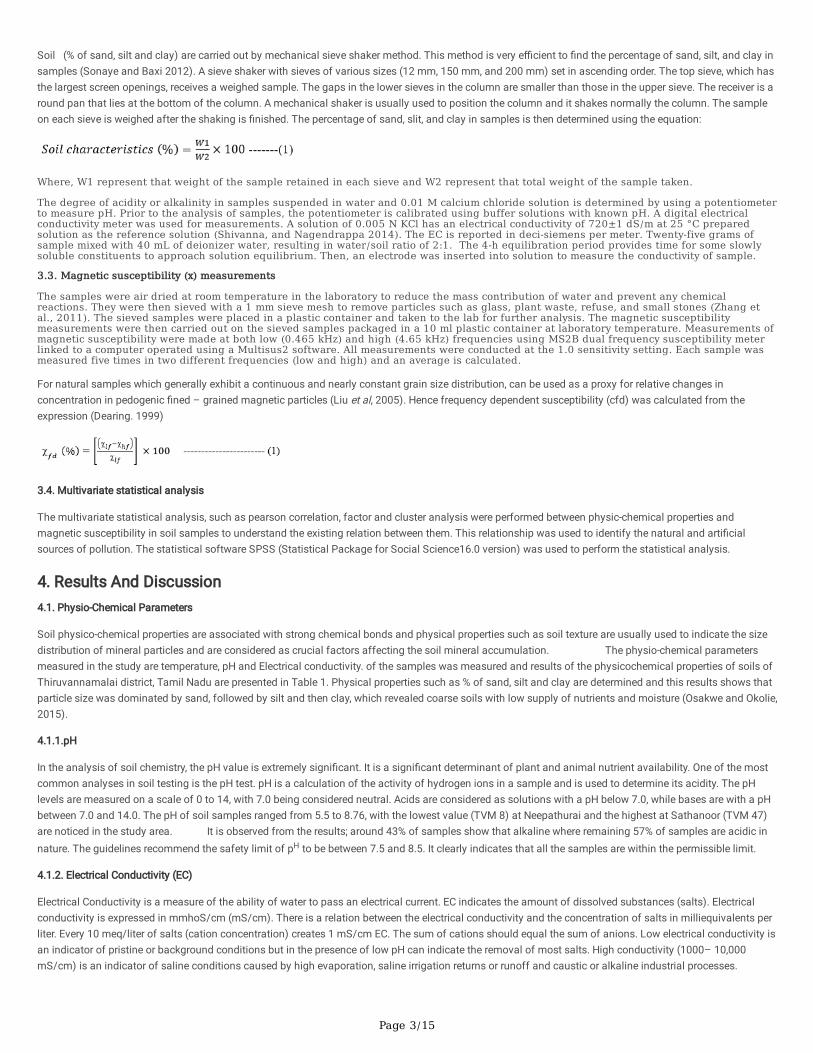
Soil   (% of sand, silt and clay) are carried out by mechanical sieve shaker method. This method is very e�cient to �nd the percentage of sand, silt, and clay insamples (Sonaye and Baxi 2012). A sieve shaker with sieves of various sizes (12 mm, 150 mm, and 200 mm) set in ascending order. The top sieve, which hasthe largest screen openings, receives a weighed sample. The gaps in the lower sieves in the column are smaller than those in the upper sieve. The receiver is around pan that lies at the bottom of the column. A mechanical shaker is usually used to position the column and it shakes normally the column. The sampleon each sieve is weighed after the shaking is �nished. The percentage of sand, slit, and clay in samples is then determined using the equation:

Where, W1 represent that weight of the sample retained in each sieve and W2 represent that total weight of the sample taken. 

The degree of acidity or alkalinity in samples suspended in water and 0.01 M calcium chloride solution is determined by using a potentiometerto measure pH. Prior to the analysis of samples, the potentiometer is calibrated using buffer solutions with known pH. A digital electricalconductivity meter was used for measurements. A solution of 0.005 N KCl has an electrical conductivity of 720±1 dS/m at 25 °C preparedsolution as the reference solution (Shivanna, and Nagendrappa 2014). The EC is reported in deci-siemens per meter. Twenty-five grams ofsample mixed with 40 mL of deionizer water, resulting in water/soil ratio of 2:1.  The 4-h equilibration period provides time for some slowlysoluble constituents to approach solution equilibrium. Then, an electrode was inserted into solution to measure the conductivity of sample.

3.3. Magnetic susceptibility (x) measurements

The samples were air dried at room temperature in the laboratory to reduce the mass contribution of water and prevent any chemicalreactions. They were then sieved with a 1 mm sieve mesh to remove particles such as glass, plant waste, refuse, and small stones (Zhang etal., 2011). The sieved samples were placed in a plastic container and taken to the lab for further analysis. The magnetic susceptibilitymeasurements were then carried out on the sieved samples packaged in a 10 ml plastic container at laboratory temperature. Measurements ofmagnetic susceptibility were made at both low (0.465 kHz) and high (4.65 kHz) frequencies using MS2B dual frequency susceptibility meterlinked to a computer operated using a Multisus2 software. All measurements were conducted at the 1.0 sensitivity setting. Each sample wasmeasured five times in two different frequencies (low and high) and an average is calculated. 

For natural samples which generally exhibit a continuous and nearly constant grain size distribution, can be used as a proxy for relative changes inconcentration in pedogenic �ned – grained magnetic particles (Liu et al, 2005). Hence frequency dependent susceptibility (cfd) was calculated from theexpression (Dearing. 1999)

3.4. Multivariate statistical analysis

The multivariate statistical analysis, such as pearson correlation, factor and cluster analysis were performed between physic-chemical properties andmagnetic susceptibility in soil samples to understand the existing relation between them. This relationship was used to identify the natural and arti�cialsources of pollution. The statistical software SPSS (Statistical Package for Social Science16.0 version) was used to perform the statistical analysis. 

4. Results And Discussion4.1. Physio-Chemical Parameters

Soil physico-chemical properties are associated with strong chemical bonds and physical properties such as soil texture are usually used to indicate the sizedistribution of mineral particles and are considered as crucial factors affecting the soil mineral accumulation.                     The physio-chemical parametersmeasured in the study are temperature, pH and Electrical conductivity. of the samples was measured and results of the physicochemical properties of soils ofThiruvannamalai district, Tamil Nadu are presented in Table 1. Physical properties such as % of sand, silt and clay are determined and this results shows thatparticle size was dominated by sand, followed by silt and then clay, which revealed coarse soils with low supply of nutrients and moisture (Osakwe and Okolie,2015).

4.1.1.pH

In the analysis of soil chemistry, the pH value is extremely signi�cant. It is a signi�cant determinant of plant and animal nutrient availability. One of the mostcommon analyses in soil testing is the pH test. pH is a calculation of the activity of hydrogen ions in a sample and is used to determine its acidity. The pHlevels are measured on a scale of 0 to 14, with 7.0 being considered neutral. Acids are considered as solutions with a pH below 7.0, while bases are with a pHbetween 7.0 and 14.0. The pH of soil samples ranged from 5.5 to 8.76, with the lowest value (TVM 8) at Neepathurai and the highest at Sathanoor (TVM 47)are noticed in the study area.             It is observed from the results; around 43% of samples show that alkaline where remaining 57% of samples are acidic innature. The guidelines recommend the safety limit of pH to be between 7.5 and 8.5. It clearly indicates that all the samples are within the permissible limit. 

4.1.2. Electrical Conductivity (EC)

Electrical Conductivity is a measure of the ability of water to pass an electrical current. EC indicates the amount of dissolved substances (salts). Electricalconductivity is expressed in mmhoS/cm (mS/cm). There is a relation between the electrical conductivity and the concentration of salts in milliequivalents perliter. Every 10 meq/liter of salts (cation concentration) creates 1 mS/cm EC. The sum of cations should equal the sum of anions. Low electrical conductivity isan indicator of pristine or background conditions but in the presence of low pH can indicate the removal of most salts. High conductivity (1000– 10,000mS/cm) is an indicator of saline conditions caused by high evaporation, saline irrigation returns or runoff and caustic or alkaline industrial processes. 

Page 4/15

In the study area electrical conductivity is found to range from 61.3 to 743 µS/cm. The values of EC measured in soil samples in the locations of Nedungavadi(TVM 46) and Randam (TVM 59) are recorded low and high values of electrical conductivity. The electrical conductivity (EC) of the soil samples ranged from61.3 to 743 (ds cm-1).  These values indicated signi�cant presence of inorganic ions in the soil (Fuller et al., 1995).

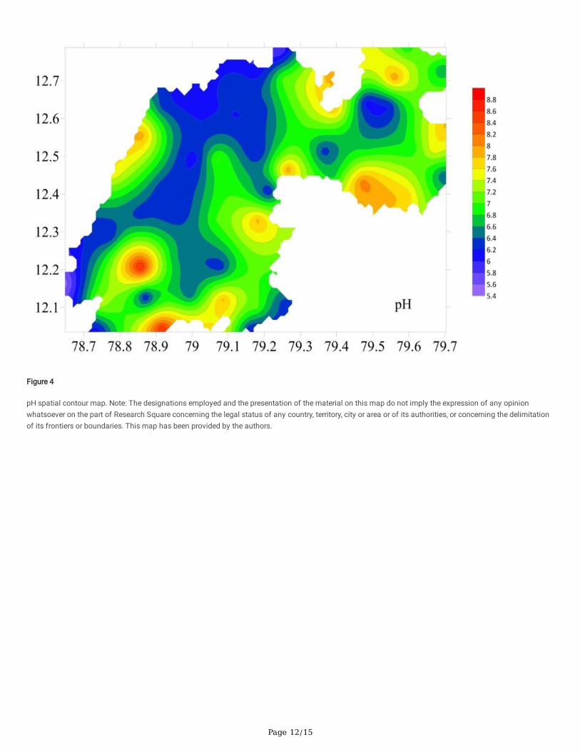
4.1.3. Spatial contouring of pH and electrical conductivity (EC)

Figure 4 and 5 plot showing a contour map superimposed on the shape of Tiruvannamlai District for pH and EC of the study area. In Figure 4 each line islabeled to identify the pH in the study area. To see the variation of EC in the sampling area a contour map has been plotted Figure 5. The contour lines arerepresentative of EC and can be used to know the EC at any point in the map.

4.1.3. Sand, Slit and Clay Analysis

Table 1 shows the results of the sand, silt, clay, and physicochemical parameters. Sand percentages range from 61% to 90%, with an average of 76.46 percentamong all stations. When compared to slilt and clay in the study area, sand is the most abundant constituent in all sampling locations. The high percentageof sand in the Seangadi (TVM 21) location could indicate a high content of quartz, whereas the lowest percentage of sand in the Nedungavadi (TVM 46)location indicated a low content of light minerals in the study region (Ravisankar et al 2019). The concentrations of silt range from 7% to 27 percent, with anaverage of 15.15 percent. Nedungavadi (TVM 46) has a high percentage of slit, which may be attributed to the primary minerals (Lal and Shukla, 2004). Theclay content varies from 2% to 16%, with an average of 8.38 percent. The high clay content in Pudhupattu (TVM 5) suggests that the soil samples containmore organic carbon.

4.1.4. Piper diagram for grain Size Analysis

A.M. developed a piper diagram in 1953 with the aim of classifying the studied quantities based on the parameters of interest. Many different computerprogrammes, such as Aqua chem and Grapher, are available on the market to plot piper diagrams. The piper diagram of slit, sand, and clay was drawn usingGrapher 14 in this analysis. The 63 samples from the study are plotted in Figure 6.  As seen by the diamond in the piper diagrams, all of the samples arecategorized as sand, slit, or clay. As compared to slit or clay, sand is the most dominant shape in the triangle. The piper diagram, which demonstrates thatsand is the key composition of soil in the study region, clearly establishes the grain size analysis of soil samples.

4.2. Magnetic susceptibilities in soils

Table 1 shows the magnetic susceptibility values for top-soil samples taken in the study region. Low frequency magnetic susceptibility values range from23.25 × 10−5 m3 kg−1 to 1664.9 × 10−5m3 kg−1 with an average value of 273.39 ×10−5m3kg−1. Low frequency magnetic susceptibility measurements showhigher results than high frequency magnetic susceptibility measurements in all soil samples. This signi�cant magnetic enhancement indicates that the soilcontains a high concentration of ferromagnetic minerals, resulting in increased pollution (Jordanova et al, 2003, Hu et al, 2007, Yang et al, 2007).Anthropogenic magnetic mineral inputs are responsible for the higher magnetic enhancement in soil samples. Vehicle emissions (vehicular exhaust,absorption) are likely sources of anthropogenic magnetic particles. Different fractions of particles produced in exhaust pipes and released into theatmosphere make up vehicular emissions.

4.3. Percentage frequency dependent susceptibility

Percentage frequency dependent susceptibility %FD is used to approximate the total concentration of SP grains, while coarse multi domain (MD) magneticgrains are frequency independent as they show similar susceptibility values at low and high frequencies. Dearing (1999) proposed a model for theinterpretation of frequency dependence as follows:  FD (%) value Interpretation Low FD (%) < 2.0% virtually no SP grains; Medium FD (%) 2.0– 10.0 %Admixture of SP and coarser non-SP grains or SP; High FD (%) 10.0 – 14.0% virtually all               (> 75%) SP grains Very high FD (%) >14 % Rare values,erroneous measurements, weak samples or contamination. Based on the semi quantitative model above, the results of this work demonstrated that most ofthe samples (about 64%) have a virtually no SP grains in the samples and remaining 36% of samples shows that admixture of SP and coarser non-SP grains. The sample TVM 45 shows the high value of %FD indicates virtually all (> 75%) SP grains and TVM 50 has the %FD 22.07 value reveals that highcontamination by magnetic mineral in the soil samples

4.4. Pearson correlation analysis  

Correlation is a bi-variate analysis that determines the strength of association between two variables. The value of the correlation coe�cient ranges between+1 and -1 in terms of the strength of the relationship. A value of ± 1 indicated that the two variables are perfectly associated (Senthil kumar et al.,2020;Harikrishan et al., 2018). The relationship between the two variables would become weaker as the correlation coe�cient value shows zero. The sign ofthe coe�cient indicates the relationship's direction; a + sign indicates a positive relationship, while a - sign indicates a negative relationship. Table 2 shows theresults of correlation analysis on physico-chemical properties and magnetic susceptibilities parameters in this study. The percentages of silt and clay indicatea clear negative relationship with the percentage of sand. This means that soil samples in the study area only contain the maximum percentage of sand. Ascan be seen from table, a weak positive correlation was observed between LF (r=0.111), HF (r=0.111) and % of sand whereas LF and HF shows that it has aweak negative correlation with % of silt, clay, EC and pH. This represented that % of sand content enhance the level of magnetic minerals in the soil samples. 

4.5 Factor analysis (FA)

Factor analysis was performed for compressing a large amount of data into a smaller, more manageable and understandable set. FA successfully helps theanalysis of meaningful information by extracting meaningful information from raw data by using established correlations among various parameters that arebeing observed (Chaturvedi and Raghubanshi 2015). FA technique �nds relationships between variables by extracting eigen values and eigen vectors from the

Page 5/15

covariance matrix of original variables, thus reducing the dimensionality of the data set. Table 3 displays the varimax rotated factor variables for physico-chemical properties and magnetic susceptibilities. Factor I and Factor II, as shown in the table -3, were extracted from the data set and explained about 78.5percent of the total variability. Factor I has a variance extraction of 26.65%, which is mostly due to high positive loadings of percent sand, LF, and HF, whileFactor II has a variance extraction of 14.20 percent due to percent silt, clay, EC, pH, and percent FD loads. These results are good agreement with correlationanalysis. 

4.6. Cluster analysis (CA)

Cluster Analysis multivariate technique in which clusters are created in a sequential manner, starting with the most similar pair of objects and moving tohigher clusters. A distance can be represented by the difference between analytical values from both samples, and the Euclidean distance normally indicateshow close two samples are (Otto 1998).The average linkage method was used to perform this technique on the normalised data collection, with Euclideandistances as a measure of similarity. This analysis examines the distances between clusters using the analysis of variance approach, attempting to minimisethe number of squares of any two clusters that can be generated at each steps. Figure 7 shows the derived dentogram of two clusters. Cluster I derived due to% of sand, silt, clay, pH, EC and %FD. Cluster II derived due to LF and HF. This means that magnetic susceptibilities are primarily related to the amount of sandin soil samples.

5. ConclusionThis paper presents the result of magnetic susceptibility and Physico-chemical properties of topsoils in different areas of Tiruvannamalai district  of  varioushuman activity locations. The results of the work shows that particle size was dominated by sand, followed by silt and then clay in samples and 57% ofsamples are acidic in nature. The results of the percentage frequency dependence showed that most of the samples have a virtually no SP grains henceobserved magnetic susceptibility values results from a combination of pedogenic and anthropogenic sources. Statistical results reveals that % of sand mainlyassociated with the low and high frequency magnetic susceptibilities in the soil samples. 

ReferencesBouhsane N., and Bouhlassa S. (2018). Assessing Magnetic Susceptibility Pro�les of Topsoils under Different Occupations. International Journal ofGeophysics. 2018,1-8.

Canbay M. 2010 Investigation of the relation between heavy metal contamination of soil and its magnetic susceptibility International Journal of Physicalsciences 5 393–400

Chaturvedi, R. K., and Raghubanshi, A. S. (2015). Assessment of carbon density and accumulation in mono-and multi-speci�c stands in Teak and Sal forestsof a tropical dry region in India. Forest Ecology and Management. 339, 11–21.

Dearing J. A., Dann R. J. L, Hay K. (1996). “Frequency-dependent susceptibility measurements of environmental materials,” Geophysical Journal International,124(1) 228–240.

Dearing J.A., 1999, Environmental Magnetic Susceptibility, Using the Bartington MS2 System. Second edition, England: Chi Publishing.

DSH, (District Statistical Handbook) (2018-2019). Department of Economics and Statistics, Tiruvannamalai, Government of Tamil Nadu; released by theDistrict Collectorate, Tiruvannamalai District, Tamil Nadu.

Durai Ganesh, Eswaran, P, Senthilkukmar, G, Bramha, S.N., Chandrasekaran, S, Ravisankar. R, (2020) A Quantitative study of Natural Uranium Present inGround Water of Tiruvannamalai district of India Iranian Journal of Science and Technology, Transactions A: Science. 45,545-555.

Geological Survey of India’s Website, Government of India, http://bukosh.gsi.gov.in/Bhukosh

Fuller MA., Feamebough W., Mitchel D., Trueman IC. (1995). Desert reclamation using Yellow River irrigation water in Ningxia, China. Soil Use Manage. 11, 77-83. 

Harikrishnan, N., Chandrasekaran, A., Ravisankar, R., & Alagarsamy, R. (2018). Statistical assessment to magnetic susceptibility and heavy metal data forcharacterizing the coastal sediment of East coast of Tamilnadu, India. Applied Radiation and Isotopes, 135, 177–183. 

HuXF., Su Y., Ye R., LiXQ and ZhangGL. (2007). Magnetic properties of the urban soils in Shanghai and their environmental implications Catena. 70, 428–36.

Jordanova NV., Jordanova DV., Veneva L., Yorova K and Petrovsky E. (2003). Magnetic response of soils and vegetation to heavy metal pollution. A case studyEnviron SciTechnol . 37, 4417–24.

Lal R., Shukla M.K. (2004), Principles of Soil Physics. Marcel Dekker, New York.

Liu Q., Torrent J., Maher B. A. (2005). “Quantifying grain size distribution of pedogenic magnetic particles in Chinese loess and its signi�cancefor pedogenesis,” Journal of Geophysical Research: Solid Earth, 110, B11102,1-7.

Page 6/15

Maher B. A. (1986).  Characterisation of soils by mineral magnetic measurements. Physics of the Earth and Planetary Interiors. 42(1-2), 76–92.

Newson M. Environmental magnetism by Roy _ompson and Frank Old�eld, vol. 13, Allen and Unwin, London, UK, 1988. 

Osakwe SA., Okolie LP. (2015). Physicochemical characteristics and heavy metals contents in soils and cassava plants from farmlands along a majorhighway in Delta State, Nigeria. J. Appl. Sci. Environ. Manage. 19(4), 695-704. 

Otto, M. (1998). Multivariate methods. In R. Kellner, J. M. Mermet, M. Otto, & H. M.Widmer (Eds.), Analytical chemistry. Weinheim: WileyeVCH.

Ramasamy V, Paramasivam K, Suresh G, Jose MT (2014) Role of sediment characteristics on natural radiation level of the Vaigai river sediment, Tamilnadu,India. J Environ Radioact 127:64–74

 Ravisankar, R., Sivakumar, S., Chandrasekaran,A., Kanagasabapathy, K.V., Prasad, M.V.R., Satapathy, K.K. 2015.  Statistical assessment of heavy metalpollution in sediments of east coast of Tamilnadu using Energy Dispersive X-ray Fluorescence Spectroscopy (EDXRF),   Applied Radiation and Isotopes, 102,42–47. 

Ravisankar R, Tholkappain M, Chandrasekaran A, Eswaran, P., Atef El-Taher (2019) Effects of Physico chemical properties on heavy metal, magneticsusceptibility and natural radionuclides in Chennai coastal sediment of East Coast of Tamilnadu, Applied Water Science, 9: 151.

Report No ESSO/IMD/HS/R.F. REPORT/02 (2014)/18, Rainfall statistics of India 2013, IndiaMeteorological Department (Ministry of Earth Sciences) by Dr.(Mrs.) Surinder Kaur and M.K. Purohit.

Sadiki A., Faleh A., Navas A., andBouhlassa S. (2009). Usingmagnetic susceptibility to assess soil degradation in the Eastern Rif, Morocco. Earth SurfaceProcesses and Landforms., 34(15), 2057–2069.

Senthil Kumar C. K., Chandrasekaran A.  (2020) Multivariate statistical tool to analyse the environmental magnetic data in Ponnai River Sand, TamilNadu Environmental Earth Sciences.  79,497. DOI: 10.1007/s12665-020-09241-7. 

Shivanna AM, Nagendrappa G (2014) Chemical analysis of soil samples to evaluate the soil fertility status of selected command areas of three tanks in TipturTaluk of Karnataka, India. IOSR J Appl Chem 7(11):01–05.

Sonaye SY, Baxi RN (2012) Particle size measurement and analysis of �our. Int J Eng Res Appl 2(3):1839–1842

Yang T., Liu Q., Chan L and Cao G. (2007). Magnetic investigation of heavy metals contamination in urban topsoils around the East Lake, Wuhan, ChinaGeophys. J. Int. 171 603–12.

Zhang C., Qiao Q., Piper J.D.A., Huang B. (2011): Assess ment of heavy metal pollution from a Fe-smelting plant in urban river sediments using environmentalmagnetic and geochemical methods. Environmental Pollution, 159: 3057–3070.

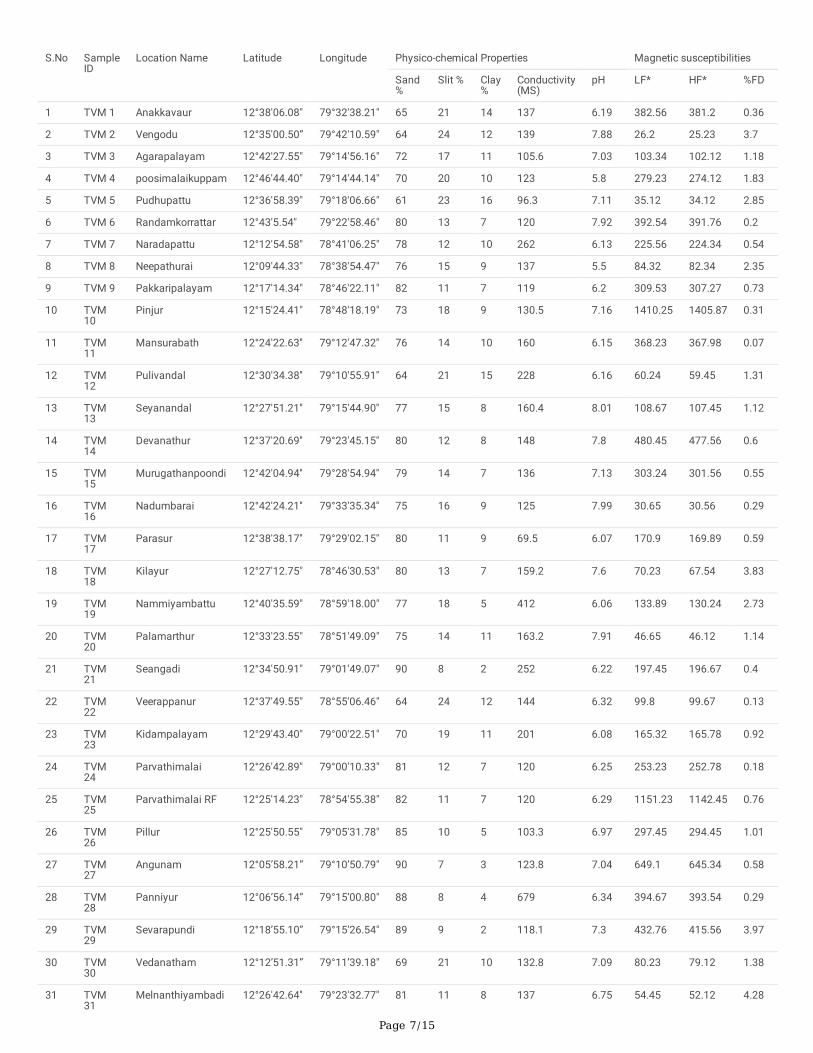
TablesTable 1 Physico-chemical properties and Magnetic susceptibilities in soils of Tiruvannamalai district, Tamil Nadu

Page 7/15

S.No SampleID

Location Name Latitude Longitude Physico-chemical Properties Magnetic susceptibilities

Sand%

Slit % Clay%

Conductivity(MS)

pH LF*  HF* %FD

1 TVM 1 Anakkavaur 12°38'06.08" 79°32'38.21" 65 21 14 137 6.19 382.56 381.2 0.36

2 TVM 2 Vengodu 12°35'00.50” 79°42'10.59" 64 24 12 139 7.88 26.2 25.23 3.7

3 TVM 3 Agarapalayam 12°42'27.55" 79°14'56.16" 72 17 11 105.6 7.03 103.34 102.12 1.18

4 TVM 4 poosimalaikuppam 12°46'44.40" 79°14'44.14" 70 20 10 123 5.8 279.23 274.12 1.83

5 TVM 5 Pudhupattu 12°36'58.39" 79°18'06.66" 61 23 16 96.3 7.11 35.12 34.12 2.85

6 TVM 6 Randamkorrattar 12°43'5.54" 79°22'58.46" 80 13 7 120 7.92 392.54 391.76 0.2

7 TVM 7 Naradapattu 12°12'54.58" 78°41'06.25" 78 12 10 262 6.13 225.56 224.34 0.54

8 TVM 8 Neepathurai 12°09'44.33" 78°38'54.47" 76 15 9 137 5.5 84.32 82.34 2.35

9 TVM 9 Pakkaripalayam 12°17'14.34" 78°46'22.11" 82 11 7 119 6.2 309.53 307.27 0.73

10 TVM10

Pinjur 12°15'24.41" 78°48'18.19" 73 18 9 130.5 7.16 1410.25 1405.87 0.31

11 TVM11

Mansurabath 12°24'22.63'' 79°12'47.32'' 76 14 10 160 6.15 368.23 367.98 0.07

12 TVM12

Pulivandal 12°30'34.38'' 79°10'55.91'' 64 21 15 228 6.16 60.24 59.45 1.31

13 TVM13

Seyanandal 12°27'51.21'' 79°15'44.90'' 77 15 8 160.4 8.01 108.67 107.45 1.12

14 TVM14

Devanathur 12°37'20.69'' 79°23'45.15'' 80 12 8 148 7.8 480.45 477.56 0.6

15 TVM15

Murugathanpoondi 12°42'04.94'' 79°28'54.94'' 79 14 7 136 7.13 303.24 301.56 0.55

16 TVM16

Nadumbarai 12°42'24.21'' 79°33'35.34'' 75 16 9 125 7.99 30.65 30.56 0.29

17 TVM17

Parasur 12°38'38.17'' 79°29'02.15'' 80 11 9 69.5 6.07 170.9 169.89 0.59

18 TVM18

Kilayur 12°27'12.75" 78°46'30.53" 80 13 7 159.2 7.6 70.23 67.54 3.83

19 TVM19

Nammiyambattu 12°40'35.59" 78°59'18.00" 77 18 5 412 6.06 133.89 130.24 2.73

20 TVM20

Palamarthur 12°33'23.55" 78°51'49.09" 75 14 11 163.2 7.91 46.65 46.12 1.14

21 TVM21

Seangadi 12°34'50.91" 79°01'49.07" 90 8 2 252 6.22 197.45 196.67 0.4

22 TVM22

Veerappanur 12°37'49.55" 78°55'06.46" 64 24 12 144 6.32 99.8 99.67 0.13

23 TVM23

Kidampalayam 12°29'43.40" 79°00'22.51" 70 19 11 201 6.08 165.32 165.78 0.92

24 TVM24

Parvathimalai 12°26'42.89" 79°00'10.33" 81 12 7 120 6.25 253.23 252.78 0.18

25 TVM25

Parvathimalai RF 12°25'14.23" 78°54'55.38" 82 11 7 120 6.29 1151.23 1142.45 0.76

26 TVM26

Pillur 12°25'50.55" 79°05'31.78" 85 10 5 103.3 6.97 297.45 294.45 1.01

27 TVM27

Angunam 12°05’58.21” 79°10’50.79" 90 7 3 123.8 7.04 649.1 645.34 0.58

28 TVM28

Panniyur 12°06’56.14” 79°15’00.80" 88 8 4 679 6.34 394.67 393.54 0.29

29 TVM29

Sevarapundi 12°18’55.10” 79°15’26.54" 89 9 2 118.1 7.3 432.76 415.56 3.97

30 TVM30

Vedanatham 12°12’51.31” 79°11’39.18" 69 21 10 132.8 7.09 80.23 79.12 1.38

31 TVM31

Melnanthiyambadi 12°26'42.64'' 79°23'32.77'' 81 11 8 137 6.75 54.45 52.12 4.28

Page 8/15

32 TVM32

Melpoondi 12°30'50.70'' 79°21'57.89'' 82 14 4 212 6.27 211.56 210.9 0.31

33 TVM33

Vallam 12°31'16.88'' 79°29'05.69'' 86 9 5 72.4 6.75 1173.56 1171.23 0.2

34 TVM34

Kanji 12°21'14.60" 78°57'41.36" 65 20 15 118 6.2 101.12 98.56 2.53

35 TVM35

Monnormangalam 12°20'39.79" 78°51'13.91" 88 9 3 233 6.3 24.13 24.08 0.21

36 TVM36

Ananthapuram 12°41'14.54" 79°07'25.22" 66 22 12 97.8 6.42 109.14 108.67 0.43

37 TVM37

Edaipirai 12°29'42.32" 79°04'11.39" 88 9 3 89.3 7.06 58.45 57.65 1.37

38 TVM38

Illupakkam 12°37'30.87" 79°11'58.18" 68 20 12 112 6.32 1664.9 1648 1.02

39 TVM39

Thurinjikuppam 12°36'32.79" 79°07'17.97" 73 17 10 140 6.18 35.67 34.34 3.73

40 TVM40

Seeyamangalam 12°25'54.09'' 79°28'15.03'' 88 8 4 152 8.13 69.89 67.78 3.02

41 TVM41

Theyyar 12°23'37.51'' 79°35'40.43'' 65 21 14 144 7.75 23.25 22.76 2.11

42 TVM42

Beemarapati 12°02'27.18''

78°44'32.70'' 72 17 11 118 6.12 921.78 905.89 1.72

43 TVM43

Kuvilam 12°02'46.38'' 78°54'51.39'' 85 12 3 94.3 8.61 83.89 80.89 3.58

44 TVM44

Malamanjanur 12°07'38.58''

78°52'13.71'' 71 19 10 131 6.15 162.67 161.76 0.56

45 TVM45

Melpasar 12°06'22.15''

78°44'33.54'' 64 20 16 117.1 7.32 39.67 35.65 10.13

46 TVM46

Nedungavadi 12°13'52.46'' 78°56'50.23'' 61 27 12 61.3 6.68 52.78 49.43 6.35

47 TVM47

Sathanoor 12°12'22.88''

78°51'27.46'' 70 20 10 109.2 8.76 56.89 52.5 7.72

48 TVM48

Vakkilapattu 12°07'46.85'' 78°59'37.26'' 81 12 7 712.04 6.45 23.5 22.34 4.94

49 TVM49

Devanur 12°02'05.48" 79°05'25.13" 80 12 8 112.1 7.47 39.12 36.76 6.03

50 TVM50

Kattompoondi 12°07'16.08" 79°05'02.03" 81 15 4 78.5 7.86 25.78 20.09 22.07

51 TVM51

Melathikam 12°12'25.79" 79°04'46.54" 69 20 11 709 6.26 166.12 164.43 1.02

52 TVM52

Virthuvilanginan 12°02'23.12" 79°09'38.20" 65 22 13 122 6.12 480.67 477.41 0.68

53 TVM53

Karunthuvambadi 12°19'49.27" 79°03'50.62" 75 16 9 83.9 7 32.56 32.45 0.34

54 TVM54

Mangalam 12°19'48.33" 79°10'57.77" 87 9 4 282 7.89 99.9 95.45 4.45

55 TVM55

Badhur 12°26'56.57'' 79°41'39.92'' 88 10 2 113.2 6.41 569.76 568.12 0.29

56 TVM56

Vazhur 12°30'59.93'' 79°40'13.52'' 72 18 10 108.8 7.55 85.12 82.34 3.27

57 TVM57

Vengunam 12°31'12.10'' 79°36'30.36'' 86 11 3 83.7 6.87 63.34 61.01 3.68

58 TVM58

Abdullapuram 12°47'03.42" 79°40'25.24" 69 19 12 108.5 7.42 37.23 36.78 1.21

59 TVM59

Randam 12°47'15.45" 79°28'13.28" 84 10 6 743 7.56 457.09 453.78 0.72

60 TVM60

Sodiambakkam 12°43'39.32" 79°41'22.92" 69 20 11 71 6.6 410.89 402.1 2.14

61 TVM Vembakkam 12°47'12.71" 79°35'27.77" 80 12 8 92.3 6.84 523.76 518.76 0.95

Page 9/15

61

62 TVM62

Devikapuram 12°29'43.73" 79°15'11.49" 79 15 6 413.01 7.22 475.08 473.67 0.3

63 TVM63

Ramasanikuppam 12°43'13.15" 79°10'35.56" 87 8 5 94.5 6.06 146.56 142.09 3.05

Minimum 61 7 2 61.3 5.5 23.25 20.09 0.07

Maximum 90 27 16 743 8.76 1664.9 1648 22.07

Average 76.46 15.15 8.38 177.62 6.873 273.38 270.50 2.227

Table 2 Pearson correlation analysis physico-chemical properties and magnetic susceptibilities

 Variables Sand % Silt % Clay % EC pH LF*  HF* %FD

Sand % 1              

Slit % -0.969 1            

Clay % -0.944 0.833 1          

EC 0.166 -0.159 -0.158 1        

pH 0.106 -0.078 -0.133 -0.111 1      

LF*  0.111 -0.123 -0.084 -0.045 -0.191 1    

HF* 0.111 -0.124 -0.084 -0.044 -0.191 1.000 1  

%FD -0.050 0.101 -0.022 -0.108 0.335 -0.290 -0.293 1.000

Table 3 Factor analysis of physico-chemical properties and magnetic susceptibilities

Variables Factors

1 2

Sand % 0.093 0.182

Slit % -0.105 -0.178

Clay % -0.067 -0.171

EC -0.150 0.989

pH -0.177 -0.139

LF*  0.994 0.105

HF* 0.994 0.107

%FD -0.277 -0.152

% of variance explained  26.65 14.20

 

Figures

Page 10/15

Figure 1

Location of the study area - Tiruvannamalai District. Note: The designations employed and the presentation of the material on this map do not imply theexpression of any opinion whatsoever on the part of Research Square concerning the legal status of any country, territory, city or area or of its authorities, orconcerning the delimitation of its frontiers or boundaries. This map has been provided by the authors.

Figure 2

Page 11/15

Sampling Sites with GPS Coordinates within the grids. Note: The designations employed and the presentation of the material on this map do not imply theexpression of any opinion whatsoever on the part of Research Square concerning the legal status of any country, territory, city or area or of its authorities, orconcerning the delimitation of its frontiers or boundaries. This map has been provided by the authors.

Figure 3

Overlay of sampling locations on the lithology of the study area. Note: The designations employed and the presentation of the material on this map do notimply the expression of any opinion whatsoever on the part of Research Square concerning the legal status of any country, territory, city or area or of itsauthorities, or concerning the delimitation of its frontiers or boundaries. This map has been provided by the authors.

Page 12/15

Figure 4

pH spatial contour map. Note: The designations employed and the presentation of the material on this map do not imply the expression of any opinionwhatsoever on the part of Research Square concerning the legal status of any country, territory, city or area or of its authorities, or concerning the delimitationof its frontiers or boundaries. This map has been provided by the authors.

Page 13/15

Figure 5

Electrical conductivity. Note: The designations employed and the presentation of the material on this map do not imply the expression of any opinionwhatsoever on the part of Research Square concerning the legal status of any country, territory, city or area or of its authorities, or concerning the delimitationof its frontiers or boundaries. This map has been provided by the authors.

Page 14/15

Figure 6

Piper diagram of grain size analysis

Page 15/15

Figure 7

Dendrogram of cluster analysis