MADES-248864-D3.2 - Models and methods for systems environment v1api.ning.com/files/*MVnc9iSFPecGVS1rteaKUtxK1... · 2017-05-27 · D3.2 Models and Methods for Systems' Environment

D3.2 Models and Methods for Systems' Environment 2/2/2011

The research leading to these results has received funding from the European Community's Seventh Framework Programme (FP7/2007-2013) under grant agreement n° 248864.

MADES

Model-based methods and tools for Avionics and surveillance embeddeD SystEmS

FP7-ICT-2007 248864

D3.2 Models and Methods for Systems' Environment

Work package: WP3 Lead participant: POLIMI Editor: Filippo Donida, Matteo Rossi Authors: Luciano Baresi, Francesco Casella, Filippo Donida,

Gianni Ferretti, Alberto Leva, Matteo Rossi Reviewers: Richard Paige, Alessandra Bagnato Date: 31/1/2011 Version: 1.0

Dissemination level

PU Public X

PP Restricted to other programme participants (including Commission Services)

RE Restricted by a group specified by the consortium (including Commission Services)

CO Confidential, only for members of the consortium (including Commission Services)


2(28)

The MADES Consortium

TXT e-solutions

Via Frigia 27 20126 Milano Italy

Contact: Ms. Alessandra Bagnato E-mail: [email protected] Phone: +39 2 25771.725 Address: Via al Ponte Reale 5 16124 Genova, Italy

SOFTEAM

21 avenue Victor Hugo 75016 Paris France

Contact: Dr. Andrey Sadovykh E-mail: [email protected] Phone: +33.1.30.12.18.57

University of York Heslington York YO10 5DD United Kingdom

Contact: Prof. Richard Paige E-mail: [email protected] Phone: +44 1904 325170

Politecnico di Milano via Golgi, 42 20133 Milano Italy

Contact: Prof. Luciano Baresi E-mail: [email protected] Phone: +39 02 2399 3638

The Open Group Avenue du Parc de Woluwe 56 B-1160 Brussels Belgium

Contact: Scott Hansen E-mail: [email protected] Phone: +32 2 6751136

EADS Deutschland

Woerthstrasse 85 89077 Ulm Germany

Contact: Ms. Gundula Blohm E-mail: [email protected] Phone: +49 731 392 3757


3(28) Copyright © MADES Consortium

Table of contents

Table of contents............................................................................................................3 1 Introduction .....................................................................................................4

1.1 Role of this document......................................................................................5 1.2 Structure of this document ..............................................................................6 1.3 Relationship to other MADES deliverables ....................................................6 1.4 Contributors.....................................................................................................6

2 Integrated Simulation ......................................................................................6 3 Modelica ........................................................................................................13

3.1 Modeling principles.......................................................................................15 3.2 Libraries.........................................................................................................17

4 The MADES Approach .................................................................................18 4.1 Simulation mechanism ..................................................................................23

5 Example.........................................................................................................25 6 Conclusions ...................................................................................................26 7 References .....................................................................................................27



1 Introduction

The design of complex embedded (software) systems requires a careful analysis of all involved elements. The system-to-be must be strictly aligned with the elements it is supposed to interact with and the context in which it will operate1. Strong timing re-quirements and complex interactions with controlled elements may further complicate the design. The different natures of all these elements are difficult to address by means of a single technique/notation. The different parts require dedicated skills and also special-purpose modelling means (see also Deliverable D1.1 "Requirements Specification"). A single, all-encompassing, homogeneous, model would only provide an unnecessarily complex solution with limited significance for many of the involved professionals. In addition, very specialised and different formalisms are adopted for the requirement definition, the system specification, the functional design, the imple-mentation, the detailed design, the simulation and so on and so forth. Each step in this process is taking advantage of its own set of ad hoc designed formalism, thus imply-ing the usage of very specific tools. This is why most approaches to the design of complex embedded software systems rely on different modelling and development tools for the software system and for the environment. This fact leads naturally to im-plement cosimulation mechanisms in order to assess the overall behaviour of an em-bedded software system coupled with a dynamic model of the environment. Cosimu-lation [HB97] is a methodology that allows individual components to be simulated by different simulation tools running simultaneously and exchanging information in a collaborative manner. A number of tools exist to realize cosimulation among different modelling and simulation environments and different application fields. To give just an example, the Siemens PLM2 for machine tools implements cosimulation among the SIMULINK models of drives and control systems and the multibody model of the mechanical structure, processed by another tool.

Modelling techniques for the environment have been consolidated through the years and rely on two main and well-known conceptual approaches. In the causal approach, adopted by SIMULINK3, each component of the environment is modelled as an ODE (Ordinary Differential Equation) system and the connection among components is re-alized through input and output variables. In the acausal approach, realized by the object-oriented language Modelica4 and by the relevant interpreters, not only each component, generally modelled by a DAE (Differential Algebraic Equation) system, has a direct physical counterpart, but also the connections among components is per-formed by stating physical principles, thus by equating effort variables and by balanc-ing flow variables.

In contrast, the problem of modelling and designing the software system has been ap-proached with different techniques, characterized by complementary advantages and limitations:

•••• Informal approaches better match domain expertise, but they can be analysed only partially.

1 Hereafter we will use the term environment to refer to both the elements the system will interact with

and the context in which it will operate. 2 Product Lifecycle Management. 3 http://www.mathworks.com/products/simulink/ 4 http://www.modelica.org



•••• Formal methods can be more difficult to adapt to the problem domain, but they typically provide richer support for analysis and verification.

Although the problem of integrating different approaches for modelling, designing, and analysing embedded software systems together with the environment in which they operate has been widely studied, no conclusive solutions have been proposed yet. In this respect the EUROSYSLIB5 (ITEA 2 ~ 06020) project must be mentioned, which is aimed at making Modelica the de-facto standard language for embedded sys-tem modelling and simulation. MADES aims to provide an innovative solution by: (a) leveraging well-known modelling tools and standards, (b) hiding the formal represen-tation used for verification to domain experts, and (c) providing a comprehensive simulation environment to support what-if analyses and the run of complete scenarios.

As for the design of the software system, MADES proposes an innovative notation in deliverable D2.1 "MADES Modelling Language Specification" inspired by the UML, MARTE (Modeling and Analysis of Real-Time and Embedded Systems), and SysML (Systems Modeling Language). The definition of the environment is demanded to Modelica, a non-proprietary, and freely available, object-oriented, equation-based language widely used to conveniently model the dynamic behavior of technical sys-tems consisting of components from, e.g., mechanical, electrical, thermal, hydraulic, pneumatic, fluid, control subsystems and other domains. Models are described by dif-ferential, algebraic, and discrete equations and “executed” through different simula-tion environments.

The Modelica language provides two main advantages with respect to the other proc-ess-simulation languages: first of all Modelica – as well as its specifications – is non-proprietary and open source, meaning that a developer is not tied to a specific tool vendor; in addition, the way the model solution is calculated is totally transparent to the user, hence the modeler is not required to carry out pre-elaborations to re-describe the model in a way that is suitable for the solver. Moreover, the Modelica language allows users to describe the components as DAE (Differential Algebraic Equation) systems, while the more common commercial languages and tools for the process simulation (e.g. Matlab/Simluink) require the system to be described in the state space form (Ordinary Differential Equation), thus requiring additional effort by the devel-oper. This is not only a waste of time because of the mathematical manipulation re-quired to the user, but it is also a highly inefficient process because of the scarce re-usability. The interested reader can refer to Section 3 for additional information on the Modelica language6.

1.1 Role of this document

This document constitutes MADES project deliverable D3.2 Models and Methods for

Systems' Environment. It presents our proposal for the holistic modelling of the envi-ronment in which complex embedded systems are supposed to operate. It presents our idea of integrated simulation to provide users with a complete simulation environ-ment, and then it introduces the modelling notation selected by the project and a suit-able, lightweight modelling approach. Such an approach is lightweight in the sense that it allows designers to combine different, complementary formalisms (differential equations, logic formalisms) in a seamless manner, instead of requiring them to fit

5 http://www.eurosyslib.com/. 6 The Modelica specifications are freely available for the download at the Modelica website:

http://www.modelica.org/documents



their models to a single, all-encompassing, notation, thus leveraging the respective strengths of the involved formalisms. In addition, much of the complexity of produc-ing the actual formal model is hidden to the user thanks, on the one hand, to the ex-tensive libraries available for the Modelica language (see also Section 3), and on the other hand to the availability, in the MADES approach, of a technique for generating logic models from MADES diagrams, according to the semantics of deliverable D3.3, "Formal dynamic semantics of the modelling notation".

1.2 Structure of this document

This deliverable is structured as follows. Section 2 describes the key concepts behind the idea of integrated simulation. Section 3 provides a brief and self-contained intro-duction to the Modelica modeling notation, while Section 4 describes the approach we suggest for obtaining a proper model of the environment. Section 5 provides the mod-el of an example environment, borrowed from one of the case studies used in the pro-ject. Section 6 concludes the document.

1.3 Relationship to other MADES deliverables

This deliverable is closely related to Deliverable D3.3, "Formal dynamic semantics of the modelling notation", which describes how a discrete metric temporal logic model is derived from the notation introduced in deliverables D2.1 "D2.1 - MADES Model-ling Language Specification" and D3.1 "D3.1 - Domain-specific and user-centred ver-ification".

1.4 Contributors

Politecnico di Milano has been the major contributor to this deliverable as well the editor of the various versions of the document. Richard Paige (University of York) and Alessandra Bagnato (TXT) have acted as reviewers for the deliverable providing valuable suggestions for final editing and refinements.

2 Integrated Simulation

In a nutshell, the goal of simulation is, given models of the behaviour of the system being developed and of its environment, to produce a trace that is "compatible" with both models, i.e., that does not violate either model. By "trace" it is meant a sequence over a time interval of values, which correspond to the values assumed over that time interval by a set of quantities (or "variables") of interest (physical quantities, such as temperature, velocity, altitude, or logical ones, such as a switch being turned on or off, etc.). Suppose, for example, that the variables of interest are the temperature T in a room and the state S on/off of a fan, and that the time interval is the discrete one [0..5], then a trace could be [⟨T=25,S=off⟩0, ⟨T=26,S=off⟩1, ⟨T=27,S=on⟩2, ⟨T=28,S=on⟩3, ⟨T=27,S=on⟩4, ⟨T=27,S=on⟩5], where the subscript indicates the instant of the [0..5] interval.

Usually, the model S of the system being designed and the model E of its environment are expressed through different formalisms and using different notions of time. More precisely, the model S of the system being designed is typically described through formalisms of discrete mathematics such as automata or logics, using a discrete notion of time (in which case interval [0..5] is, as in the example above, the sequence [0, 1, 2,



3, 4, 5]); the behaviour of its physical environment E, on the other hand, is normally described through differential equations, with an underlying continuous notion of time. Then, a notion of "hybrid" simulation is necessary, one that seamlessly mixes the concepts above.

In the MADES approach, the two models S and E are rather loosely coupled, and there is not a controller-controlled relationship between them. That is, system S being designed is not the controller of E as in the classic control theory; rather, the coupling between the two models occurs simply by sharing some variables; that is, in an ap-proach that is reminiscent of the reference model presented in [GGJZ00], there is a set of variables, suitably identified in the MADES diagrams, that appear both in S and in E. Note that there need not be a notion of input/output attached to shared variables, though this is sometimes useful; more simply, shared variables are quantities over which both S and E models predicate, hence they are also the mechanism through which the two models interact in the simulation. Then, it is not a case of system S be-ing the controller and physical environment E being controlled; they exist separately, and interact by sharing some values.

In the MADES approach, the model of system S is given through the notation defined in Deliverables D2.1 and D3.1, using the semantics of Deliverable D3.3 to produce the actual formal model. The dynamics of environment E, instead, is given as a set of differential equations, according to the framework presented in Sections 3 and 4 of this deliverable.

Then, in the rest of this deliverable we will assume the system S being designed to be modelled as a set of metric temporal logic formulae, which are those obtained by ap-plying the semantics of Deliverable D3.3 to the notation of Deliverables D2.1 and D3.1.

From the considerations above, in essence the simulation activity must produce one trace made of two parts:

• One part is based on a discrete notion of time, and it is derived by applying trace-generation techniques to the metric temporal logic model S (that is, it is a trace of the variables of interest of the system being designed). A trace com-patible with a metric temporal logic model can be obtained, for example, through a tool such as Zot7, by checking for the satisfiability of a correspond-ing formula expressed in a suitable decidable logic.

• The second part is based on a continuous notion of time, and it is a trace of the physical environment E, which is produced through an interpreter of differen-tial equations such as those available for the Modelica language (see Section 3).

To integrate the two sub-traces in the same framework, we can sample the continu-ous-time trace of the physical environment E, then check that it is compatible with the discrete-time trace of system S.

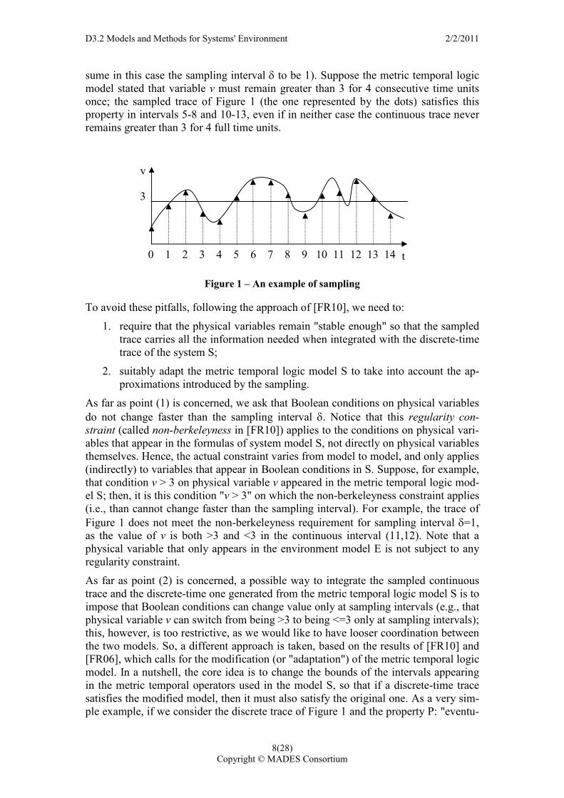
For this approach to deliver consistent results, however, the system model S cannot be used "as is" after producing it through the formal semantics of Deliverable D3.3; in-stead, it must be suitably adapted and modified according to the technique presented in the rest of this section. Consider, for example, Figure 1, which shows a trace for continuous-time variable v and one of its possible samplings (for simplicity, we as- 7 http://home.dei.polimi.it/pradella/Zot



sume in this case the sampling interval δ to be 1). Suppose the metric temporal logic model stated that variable v must remain greater than 3 for 4 consecutive time units once; the sampled trace of Figure 1 (the one represented by the dots) satisfies this property in intervals 5-8 and 10-13, even if in neither case the continuous trace never remains greater than 3 for 4 full time units.

Figure 1 – An example of sampling

To avoid these pitfalls, following the approach of [FR10], we need to:

1. require that the physical variables remain "stable enough" so that the sampled trace carries all the information needed when integrated with the discrete-time trace of the system S;

2. suitably adapt the metric temporal logic model S to take into account the ap-proximations introduced by the sampling.

As far as point (1) is concerned, we ask that Boolean conditions on physical variables do not change faster than the sampling interval δ. Notice that this regularity con-straint (called non-berkeleyness in [FR10]) applies to the conditions on physical vari-ables that appear in the formulas of system model S, not directly on physical variables themselves. Hence, the actual constraint varies from model to model, and only applies (indirectly) to variables that appear in Boolean conditions in S. Suppose, for example, that condition v > 3 on physical variable v appeared in the metric temporal logic mod-el S; then, it is this condition "v > 3" on which the non-berkeleyness constraint applies (i.e., than cannot change faster than the sampling interval). For example, the trace of Figure 1 does not meet the non-berkeleyness requirement for sampling interval δ=1, as the value of v is both >3 and <3 in the continuous interval (11,12). Note that a physical variable that only appears in the environment model E is not subject to any regularity constraint.

As far as point (2) is concerned, a possible way to integrate the sampled continuous trace and the discrete-time one generated from the metric temporal logic model S is to impose that Boolean conditions can change value only at sampling intervals (e.g., that physical variable v can switch from being >3 to being <=3 only at sampling intervals); this, however, is too restrictive, as we would like to have looser coordination between the two models. So, a different approach is taken, based on the results of [FR10] and [FR06], which calls for the modification (or "adaptation") of the metric temporal logic model. In a nutshell, the core idea is to change the bounds of the intervals appearing in the metric temporal operators used in the model S, so that if a discrete-time trace satisfies the modified model, then it must also satisfy the original one. As a very sim-ple example, if we consider the discrete trace of Figure 1 and the property P: "eventu-

3

t

v

0 1 2 3 4 5 6 7 8 9 10 11 12 13 14



ally it is v > 3 for 4 consecutive time units" and change it to P': "eventually it is v > 3 for 2 consecutive time units", if P holds for a discrete-time trace τd, than P' also holds for any continuous-time trace τ'c (satisfying also the non-berkeleyness constraint) that has τd for a sampling.

More precisely, we introduce two adaptation functions, ηRδ and ηZ

δ, (which are para-metric with respect to the sampling interval δ) that have the following properties, giv-en a metric temporal logic formula F:

1. For every continuous-time trace τc that is non-berkeley for the sampling inter-val δ (i.e., in which any change in a Boolean condition cannot be followed by another change in a Boolean condition unless at least δ time units have elapsed since the last change) and such that F holds on τc, adapted formula ηR

δ(F) holds for each discrete-time trace τ'd that is a sampling (with sampling interval δ) of τc.

2. Vice-versa, adaptation function ηZδ is such that, if τd is a discrete-time trace

for which F holds, then adapted formula ηZδ(F) holds for any continuous-time

trace τ'c that is non-berkeley for the sampling interval δ such that τd is a sam-pling of τ'c (using δ as sampling interval).

The above properties for adaptation functions ηRδ and ηZ

δ hold when F is a flat for-mula (i.e., it does not include temporal operators whose subformulae also contain temporal operators8), in which negations only appear next to atomic formulas.

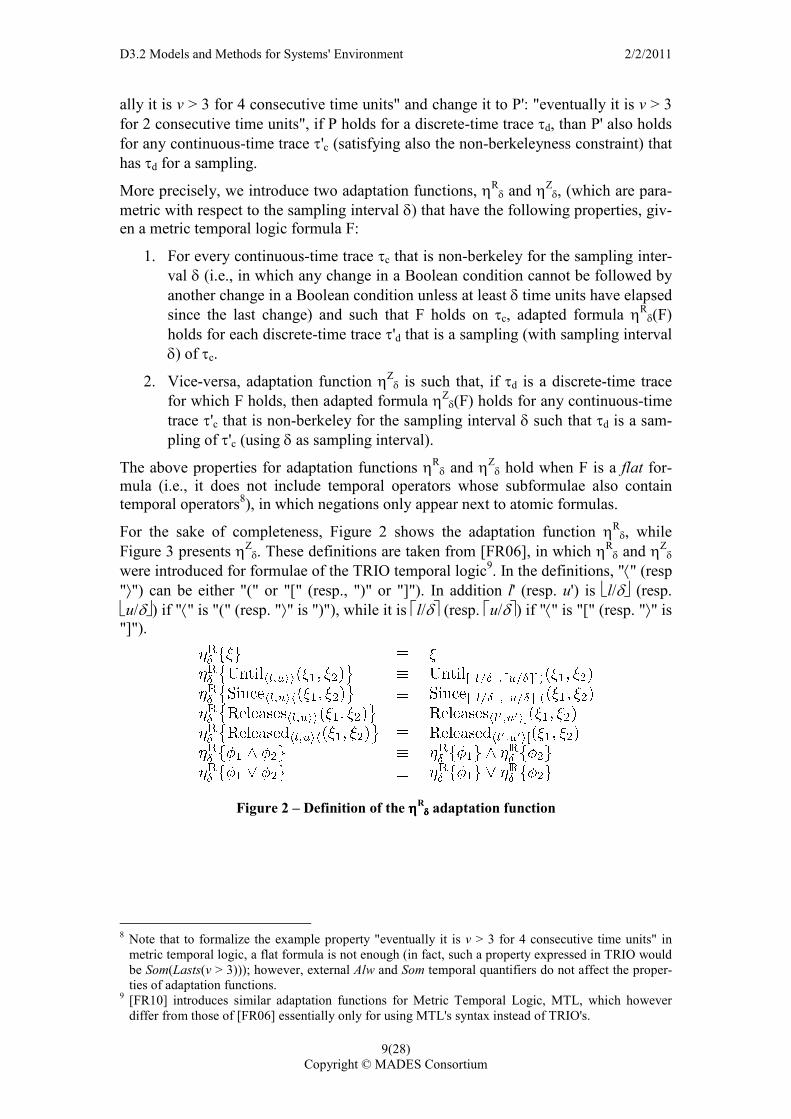
For the sake of completeness, Figure 2 shows the adaptation function ηRδ, while

Figure 3 presents ηZδ. These definitions are taken from [FR06], in which ηR

δ and ηZδ

were introduced for formulae of the TRIO temporal logic9. In the definitions, "⟨" (resp "⟩") can be either "(" or "[" (resp., ")" or "]"). In addition l' (resp. u') is l/δ (resp. u/δ) if "⟨" is "(" (resp. "⟩" is ")"), while it is l/δ (resp. u/δ) if "⟨" is "[" (resp. "⟩" is "]").

Figure 2 – Definition of the ηηηηRδδδδ adaptation function

8 Note that to formalize the example property "eventually it is v > 3 for 4 consecutive time units" in

metric temporal logic, a flat formula is not enough (in fact, such a property expressed in TRIO would be Som(Lasts(v > 3))); however, external Alw and Som temporal quantifiers do not affect the proper-ties of adaptation functions.

9 [FR10] introduces similar adaptation functions for Metric Temporal Logic, MTL, which however differ from those of [FR06] essentially only for using MTL's syntax instead of TRIO's.



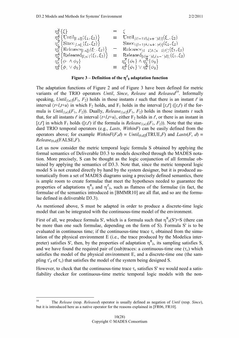
Figure 3 – Definition of the ηηηηZδδδδ adaptation function

The adaptation functions of Figure 2 and of Figure 3 have been defined for metric variants of the TRIO operators Until, Since, Release and Released10. Informally speaking, Until⟨l,u⟩](F1, F2) holds in those instants t such that there is an instant t' in interval ⟨t+l,t+u⟩ in which F2 holds, and F1 holds in the interval [t,t'] ([t,t') if the for-mula is Until⟨l,u⟩)(F1, F2)). Dually, Release⟨l,u⟩](F1, F2) holds in those instants t such that, for all instants t' in interval ⟨t+l,t+u⟩, either F2 holds in t', or there is an instant in [t,t'] in which F1 holds ([t,t') if the formula is Release⟨l,u⟩)(F1, F2)). Note that the stan-dard TRIO temporal operators (e.g., Lasts, WithinF) can be easily defined from the operators above; for example WithinF(F,d) ≡ Until(0,d]](TRUE,F) and Lasts(F, d) ≡ Release(0,d](FALSE,F).

Let us now consider the metric temporal logic formula S obtained by applying the formal semantics of Deliverable D3.3 to models described through the MADES nota-tion. More precisely, S can be thought as the logic conjunction of all formulae ob-tained by applying the semantics of D3.3. Note that, since the metric temporal logic model S is not created directly by hand by the system designer, but it is produced au-tomatically from a set of MADES diagrams using a precisely defined semantics, there is ample room to create formulae that meet the hypotheses needed to guarantee the properties of adaptations ηR

δ and ηZδ, such as flatness of the formulae (in fact, the

formulae of the semantics introduced in [BMMR10] are all flat, and so are the formu-lae defined in deliverable D3.3).

As mentioned above, S must be adapted in order to produce a discrete-time logic model that can be integrated with the continuous-time model of the environment.

First of all, we produce formula S', which is a formula such that ηRδ(S')=S (there can

be more than one such formulae, depending on the form of S). Formula S' is to be evaluated in continuous time; if the continuous-time trace τc obtained from the simu-lation of the physical environment E (i.e., the trace produced by the Modelica inter-preter) satisfies S', then, by the properties of adaptation ηR

δ, its sampling satisfies S, and we have found the required pair of (sub)traces: a continuous-time one (τc) which satisfies the model of the physical environment E, and a discrete-time one (the sam-pling τ'd of τc) that satisfies the model of the system being designed S.

However, to check that the continuous-time trace τc satisfies S' we would need a satis-fiability checker for continuous-time metric temporal logic models with the non-

10 The Release (resp. Released) operator is usually defined as negation of Until (resp. Since), but it is introduced here as a native operator for the reasons explained in [FR06, FR10].



berkeleyness constraint, which is currently not available11. Hence, a second approxi-mation is used.

More precisely, formula S' is further transformed into a metric temporal logic formula S'' which is such that ηZ

δ(S'') = S'. 12 Then, if τc exhibits the non-berkeleyness property when one considers Boolean conditions on physical variables appearing in S', and if S'' holds for the discrete-time trace τ'd obtained by sampling τc (using δ as sampling interval), we can conclude, for the properties of the adaptation function ηZ

δ, that S' holds for τc, and we have indeed obtained the two necessary (sub)traces τc and τ'd.

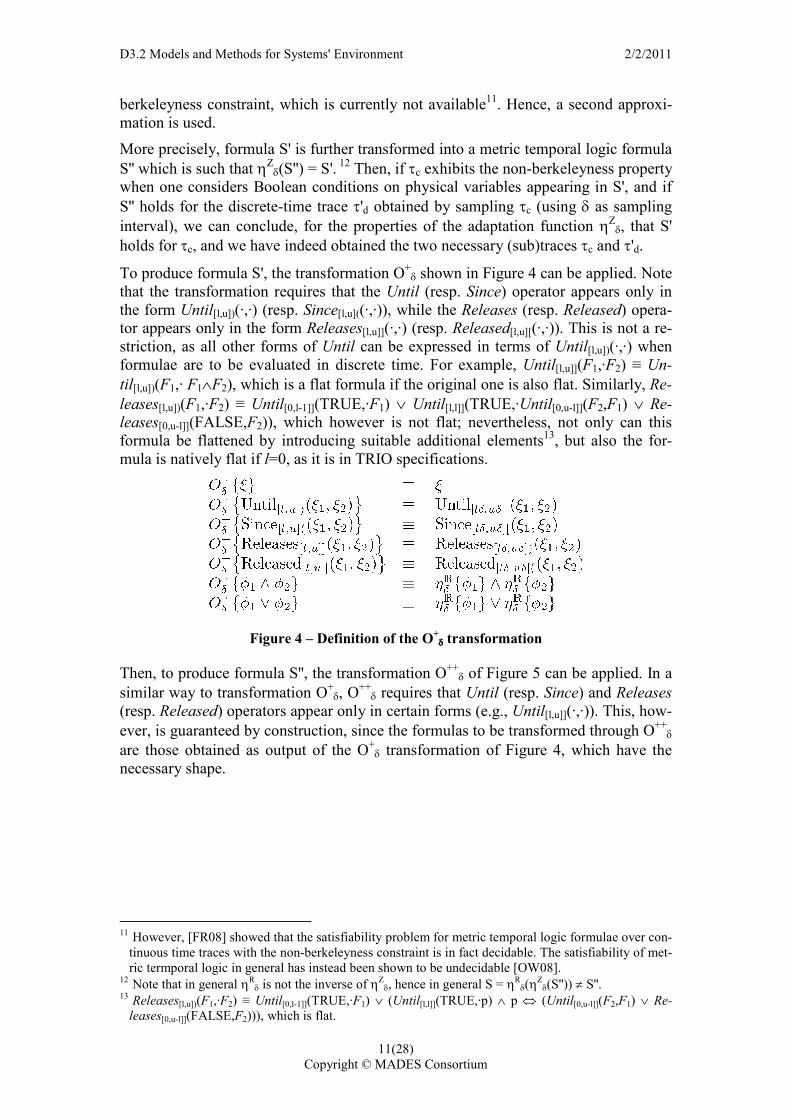
To produce formula S', the transformation O+δ shown in Figure 4 can be applied. Note

that the transformation requires that the Until (resp. Since) operator appears only in the form Until[l,u])(·,·) (resp. Since[l,u]((·,·)), while the Releases (resp. Released) opera-tor appears only in the form Releases[l,u]](·,·) (resp. Released[l,u][(·,·)). This is not a re-striction, as all other forms of Until can be expressed in terms of Until[l,u])(·,·) when formulae are to be evaluated in discrete time. For example, Until[l,u]](F1,·F2) ≡ Un-

til[l,u])(F1,· F1∧F2), which is a flat formula if the original one is also flat. Similarly, Re-leases[l,u])(F1,·F2) ≡ Until[0,l-1]](TRUE,·F1) ∨ Until[l,l]](TRUE,·Until[0,u-l]](F2,F1) ∨ Re-leases[0,u-l]](FALSE,F2)), which however is not flat; nevertheless, not only can this formula be flattened by introducing suitable additional elements13, but also the for-mula is natively flat if l=0, as it is in TRIO specifications.

Figure 4 – Definition of the O+δδδδ transformation

Then, to produce formula S'', the transformation O++δ of Figure 5 can be applied. In a

similar way to transformation O+δ, O

++δ requires that Until (resp. Since) and Releases

(resp. Released) operators appear only in certain forms (e.g., Until[l,u]](·,·)). This, how-ever, is guaranteed by construction, since the formulas to be transformed through O++

δ are those obtained as output of the O+

δ transformation of Figure 4, which have the necessary shape.

11 However, [FR08] showed that the satisfiability problem for metric temporal logic formulae over con-

tinuous time traces with the non-berkeleyness constraint is in fact decidable. The satisfiability of met-ric termporal logic in general has instead been shown to be undecidable [OW08].

12 Note that in general ηRδ is not the inverse of ηZ

δ, hence in general S = ηRδ(η

Zδ(S'')) ≠ S''.

13 Releases[l,u])(F1,·F2) ≡ Until[0,l-1]](TRUE,·F1) ∨ (Until[l,l]](TRUE,·p) ∧ p ⇔ (Until[0,u-l]](F2,F1) ∨ Re-leases[0,u-l]](FALSE,F2))), which is flat.



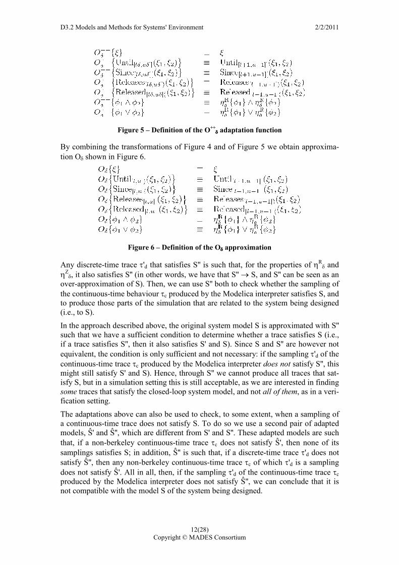
Figure 5 – Definition of the O++δδδδ adaptation function

By combining the transformations of Figure 4 and of Figure 5 we obtain approxima-tion Oδ shown in Figure 6.

Figure 6 – Definition of the Oδδδδ approximation

Any discrete-time trace τ'd that satisfies S'' is such that, for the properties of ηRδ and

ηZδ, it also satisfies S'' (in other words, we have that S'' → S, and S'' can be seen as an

over-approximation of S). Then, we can use S'' both to check whether the sampling of the continuous-time behaviour τc produced by the Modelica interpreter satisfies S, and to produce those parts of the simulation that are related to the system being designed (i.e., to S).

In the approach described above, the original system model S is approximated with S'' such that we have a sufficient condition to determine whether a trace satisfies S (i.e., if a trace satisfies S'', then it also satisfies S' and S). Since S and S'' are however not equivalent, the condition is only sufficient and not necessary: if the sampling τ'd of the continuous-time trace τc produced by the Modelica interpreter does not satisfy S'', this might still satisfy S' and S). Hence, through S'' we cannot produce all traces that sat-isfy S, but in a simulation setting this is still acceptable, as we are interested in finding some traces that satisfy the closed-loop system model, and not all of them, as in a veri-fication setting.

The adaptations above can also be used to check, to some extent, when a sampling of a continuous-time trace does not satisfy S. To do so we use a second pair of adapted models, Ŝ' and Ŝ'', which are different from S' and S''. These adapted models are such that, if a non-berkeley continuous-time trace τc does not satisfy Ŝ', then none of its samplings satisfies S; in addition, Ŝ'' is such that, if a discrete-time trace τ'd does not satisfy Ŝ'', then any non-berkeley continuous-time trace τc of which τ'd is a sampling does not satisfy Ŝ'. All in all, then, if the sampling τ'd of the continuous-time trace τc produced by the Modelica interpreter does not satisfy Ŝ'', we can conclude that it is not compatible with the model S of the system being designed.



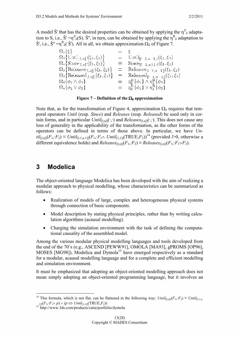
A model Ŝ' that has the desired properties can be obtained by applying the ηZδ adapta-

tion to S, i.e., Ŝ' =ηZδ(S). Ŝ'', in turn, can be obtained by applying the ηR

δ adaptation to Ŝ', i.e., Ŝ'' =ηR

δ( Ŝ'). All in all, we obtain approximation Ωδ of Figure 7.

Figure 7 – Definition of the ΩΩΩΩδδδδ approximation

Note that, as for the transformation of Figure 4, approximation Ωδ requires that tem-poral operators Until (resp. Since) and Releases (resp. Released) be used only in cer-tain forms, and in particular Until[l,u]](·,·) and Releases[l,u])(·,·). This does not cause any loss of generality in the applicability of the transformation, as the other forms of the operators can be defined in terms of those above. In particular, we have Un-

til[l,u])(F1,·F2) ≡ Until[l-1,u-1]](F1,·F1∧ Until[1,1]](TRUE,F2))14 (provided l>0, otherwise a

different equivalence holds) and Releases[l,u]](F1,·F2) ≡ Releases[l,u])(F1,·F1∨F2).

3 Modelica

The object-oriented language Modelica has been developed with the aim of realizing a modular approach to physical modelling, whose characteristics can be summarized as follows:

• Realization of models of large, complex and heterogeneous physical systems through connection of basic components.

• Model description by stating physical principles, rather than by writing calcu-lation algorithms (acausal modelling).

• Charging the simulation environment with the task of defining the computa-tional causality of the assembled model.

Among the various modular physical modelling languages and tools developed from the end of the 70’s (e.g., ASCEND [PEWW91], OMOLA [MA93], gPROMS [OP96], MOSES [MG98]), Modelica and Dymola15 have emerged respectively as a standard for a modular, acausal modelling language and for a complete and efficient modelling and simulation environment.

It must be emphasized that adopting an object-oriented modelling approach does not mean simply adopting an object-oriented programming language, but it involves an

14 This formula, which is not flat, can be flattened in the following way: Until[l,u])(F1,·F2) ≡ Until[l-1,u-

1]](F1,·F1∧ p) ∧ (p ⇔ Until[1,1]](TRUE,F2)) 15 http://www.3ds.com/products/catia/portfolio/dymola.



innovative systematic approach to the modelling task. Object-oriented modelling is then an approach to physical systems modelling based on the following key features:

• A-causal modelling. The equations of each model are written in a declarative form, i.e., by stating physical principles rather than by writing calculation al-gorithms, independently of the actual boundary conditions, and without decid-ing a-priori which are the input and which are the outputs. This results in a-causal models, described by DAE (Differential-Algebraic Equations) systems, which represent in the most natural and physically consistent way each system component. The causality of the model is determined automatically by the simulation environment at the aggregate level, when a system model is assem-bled out of elementary ones. In this way, models are much easier to write, document, and reuse, while the burden of determining the actual sequence of computations required for the simulation is entirely left to automatic symbolic manipulation tools.

• Code transparency. Equations written in a model tightly match the way they are written on paper, so that it is very easy to understand what is inside a given model, as well as modify or enhance it.

• Encapsulation. The interaction among components and (sub)models is im-plemented only through rigorously defined interfaces, called connectors, whose design is of paramount importance. A connector is defined by a set of effort variables and by a set of flow variables and the simulation environment implements a connection by equating the effort variables and by balancing the flow variables. For example, electrical connectors carry a voltage (effort) and a current (flow), thermal connectors carry a temperature (effort) and a heat flow (flow), drive train connectors an angle (effort) and a torque (flow) and so on. As long as two different components have compatible connectors, they can be bound together, regardless of their inner details. This feature is essential for the development of libraries of re-usable models; moreover, it allows users to easily replace a part of a system model with a more detailed or a more simpli-fied one, without affecting the rest of the model.

• Inheritance. Model libraries can be given a hierarchical structure, in which more complex models are obtained from basic models by adding specific vari-ables, equations or even models. For example, it is possible to write the equa-tions describing the flow of a generic gas in a tube; the model of the flow of a particular, e.g. 10-component, ideal gas mixture can be obtained by inheriting from the general one and by adding the specific model of the ideal gas.

• Multi-physics modelling. The modelling scope is general, as it provides mod-elling primitives such as generic algebraic, differential and difference equa-tions, and it is not tied to any particular engineering domain, such as mechan-ics, electrical engineering, or thermodynamics. It is then quite straightforward to model systems having a multidisciplinary nature, such as mechatronic sys-tems, resulting from the interaction of mechanical, electrical and control sub-systems, or nuclear plants, resulting from the interaction of thermo-hydraulic, nuclear and control sub-systems.

• Reusability. A-causal modelling and encapsulation are a strong incentive to-wards the development of libraries of general-purpose reusable models for dif-ferent engineering domains.



Thus, adopting such an approach, the complexity of the modelling process is confined to the development of the equations for the single components and to the definition of standardized component interfaces. Constructing a model by aggregation, or “connec-tion”, of simple components is both easy and intuitive, and generally results in a sys-tem layout similar to the physical one.

To summarize, the Modelica language is designed in such a way that the models can be assembled exactly as an engineer would build the real system: when the base com-ponents – like motors, pumps and valves – have been defined with the appropriate connectors, the main model is obtained by means of simple connections. In this sense the key point is the re-usability that is essential for handling complexity.

The Modelica language offers a suitable framework to support this approach, since it is endowed with all the object-oriented features previously listed. Modelica is suited for multi-domain modelling, including, for example, mechatronic systems in robotics, automotive and aerospace applications (with mechanical, electrical, hydraulic and control subsystems) and process-oriented applications.

3.1 Modeling principles

One of the most important properties of the Modelica language is that is a declarative language: Modelica equations are mathematical equations and not necessarily as-signments. When considering the whole system, the input/output relationships – if not specified a priori – are established dynamically just after the translation of the Mode-lica source code into a simulation executable.

A Modelica model can in general be represented graphically as a block describing the behaviour of a specific part of the physical system. In this sense, each block might interact with the rest of the model by means of connectors. Moreover, Modelica mod-els are usually connected to each other through the "connections" of the Modelica connector components, exactly as the subcomponents are physically connected to-gether in the real system. To summarize, using the Modelica "connector" concept re-sults in preserving the alignment between model representation and real system sche-mas.

In Modelica – typically when causality is known a priori (e.g. the control algorithms) – it is also possible to describe a set of causal instructions, as an algorithm section. This generally gives rise to models containing input, output and a-causal variables.

Since Modelica is an object-oriented language, the fundamental structuring unit of the modelling process is the class. Classes provide the structure for objects, also known as instances. Classes can contain equations that provide the base for the executable code that is used for computation in Modelica.

In addition, Modelica also allows the conventional algorithmic code to be part of classes. All data objects in Modelica are instantiated from classes, including the basic data types Real, Integer, String, Boolean and enumeration types, which are built-in classes.

As mentioned above, the Modelica classes – thus the Modelica models – can contain equations and algorithms to define the physical behaviour of a certain piece of the system.



Algorithms are simply standard assignments of variables, and are considered to be causal portion of code, like every assertive programming language. Unlike algorithms Modelica "equations" are acausal, since they do not directly refer to a variable as-signment. Causality is determined according to the boundary conditions of the model.

In order to make a very simple example that might help explain this concept, consider a Modelica model of a simple electric resistance. The model is obtained by writing the equation corresponding to the physical current-voltage law, that is, R*i-V=0, without regard of whether the current has to be calculated as a function of the voltage (i=V/R), or the other way around (V=i*R). The only constraint for the model developer is to ensure the mathematical correctness the specified problem: each model needs to be balanced, and the same number of variables and of equations must be present.

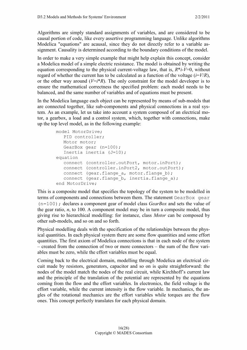
In the Modelica language each object can be represented by means of sub-models that are connected together, like sub-components and physical connections in a real sys-tem. As an example, let us take into account a system composed of an electrical mo-tor, a gearbox, a load and a control system, which, together with connections, make up the top level model, as in the following example:

model MotorDrive; PID controller; Motor motor; GearBox gear (n=100); Inertia inertia (J=10); equation connect (controller.outPort, motor.inPort); connect (controller.inPort2, motor.outPort); connect (gear.flange_a, motor.flange_b); connect (gear.flange_b, inertia.flange_a); end MotorDrive;

This is a composite model that specifies the topology of the system to be modelled in terms of components and connections between them. The statement GearBox gear (n=100); declares a component gear of model class GearBox and sets the value of the gear ratio, n, to 100. A component model may be in turn a composite model, thus giving rise to hierarchical modelling: for instance, class Motor can be composed by other sub-models, and so on and so forth.

Physical modelling deals with the specification of the relationships between the phys-ical quantities. In each physical system there are some flow quantities and some effort quantities. The first axiom of Modelica connections is that in each node of the system – created from the connection of two or more connectors – the sum of the flow vari-ables must be zero, while the effort variables must be equal.

Coming back to the electrical domain, modelling through Modelica an electrical cir-cuit made by resistors, generators, capacitor and so on is quite straightforward: the nodes of the model match the nodes of the real circuit, while Kirchhoff’s current law and the principle of the translation of the potential are represented by the equations coming from the flow and the effort variables. In electronics, the field voltage is the effort variable, while the current intensity is the flow variable. In mechanics, the an-gles of the rotational mechanics are the effort variables while torques are the flow ones. This concept perfectly translates for each physical domain.



In Modelica, the flow and effort connector variables need to be declared within spe-cific objects: the connectors. Connectors are Modelica classes containing all the quan-tities needed to describe the interaction:

connector pin Voltage v; flow Current i; end pin

connector flange Angle phi; flow Torque tau; end flange;

By default the Modelica variables declared within a connector refer to "effort" quanti-ties, unless they are declared as flow, as in the case of variable i and tau above.

A connection, e.g., connect(Pin1, Pin2), between the Pin1 and Pin2 instances of the connector class pin declared above connects the two pins such that they form a node. This implies that the following two equations are automatically generated by the compiler: 0 = Pin1.v - Pin2.v and 0 = Pin1.i + Pin2.i .The first equation indicates that voltages on both branches connected together are the same, and the second corre-sponds to Kirchhoff’s current law saying that the current sums to zero at a node. Simi-lar laws apply to mass flow rates in piping networks and to forces and torques in me-chanical systems.

Once again it is important to stress that two equations are automatically generated, rather than two assignments. The connection equation are different from the hand-written equations since they define relations between different instances of objects.

To summarize, the hand-written equations, together with the algorithms and the con-nections-generated equations, contribute to the overall mathematical model that con-stitutes the description of the system.

3.2 Libraries

Modelica classes can be grouped into packages, also called libraries, which are useful for exchanging models. There are many Modelica libraries, some of them available free of charge, while others are commercially available16.

Modelica is provided with the Modelica Standard Library which contains components from many different domains, such as:

• About 450 type definitions, such as Voltage, Angle, Inertia.

• Mathematical functions such as sin, cos, ln.

• Continuous and discrete input and output blocks, such as transfer functions, filters, sources.

• Electric and electronic components such as resistor, diode, MOS and BJT transistor.

• 1-dimensional translational components such as mass, spring, stop.

• 1-dimensional rotational components such as inertia, gearbox, bearing friction, clutch.

16 For the complete list of the Modelica libraries refer to http://www.modelica.org/libraries



• 3-dimensional mechanical components such as joints, bodies and 3-dimensional springs.

• Hydraulic components such as pumps, cylinders, valves.

• Therm-fluid flow components, such as pipes with multi-phase flow, heat ex-changers.

• 1-dimensional thermal components, such as heat resistance and heat capaci-tance.

• Power system components such as generators and lines.

• Power train components such as driver, engine, torque converter, automatic gearboxes.

4 MADES Approach

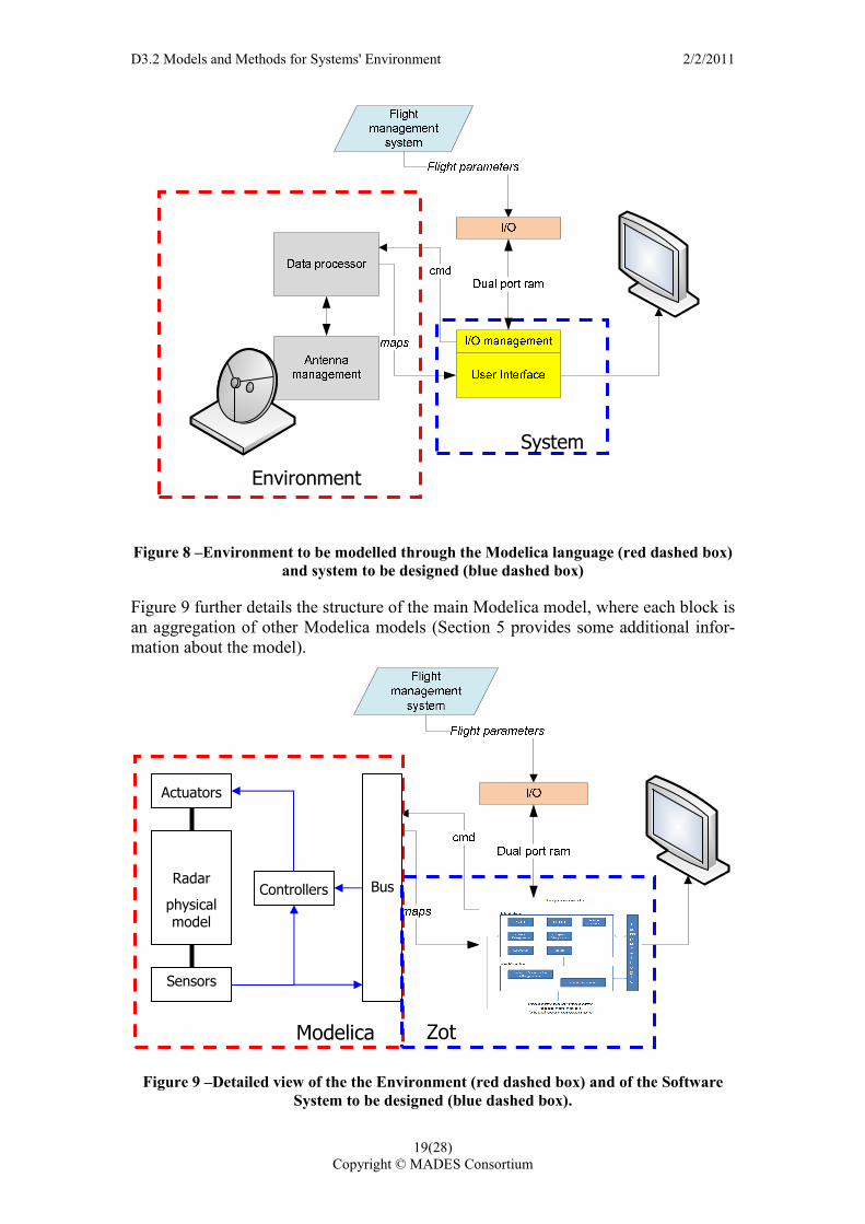
The simulation model, as mentioned in Section 2, is made of two parts: the system being designed, and its environment. Figure 8 shows a schematic high-level represen-tation of this idea, using as example an onboard radar system that is being considered by TXT as a possible case study for the MADES project. This case study focuses on the development of the user interface for a radar that is onboard a surveillance air-craft. In this example, then, the software system to be designed is the user interface, and the antenna subsystem (plus the aircraft itself) is its environment.

The environment is made up by the components within the red dashed box. This sub-system, the so-called “continuous part” of the co-simulation process, is described us-ing the Modelica language and is simulated though the commercial Dymola compiler, or through open source tools, such as OpenModelica17. It consists of the mechanical structure of the antenna, the electrical drives, the (software) control system and the sensors.

17 http://www.openmodelica.org/



Figure 8 –Environment to be modelled through the Modelica language (red dashed box)

and system to be designed (blue dashed box)

Figure 9 further details the structure of the main Modelica model, where each block is an aggregation of other Modelica models (Section 5 provides some additional infor-mation about the model).

Figure 9 –Detailed view of the the Environment (red dashed box) and of the Software

System to be designed (blue dashed box).

Modelica Zot

Radar

physical model

Actuators

Bus Controllers

Sensors

Environment

System



As shown in Figure 9, during the co-simulation process, the Modelica environment interacts with the model of the software system to be designed by means of a particu-lar Modelica connector: the Modelica bus. The Modelica bus block collects the vari-ables and signals shared by the software system and its physical environment, thus implementing the communication channel between the environment and the system model.

More precisely, a Modelica bus is an expandable connector. Expandable connectors are a particular class of Modelica connectors whose features, presented below, make them suitable and flexible enough for the data communication during the co-simulation process.

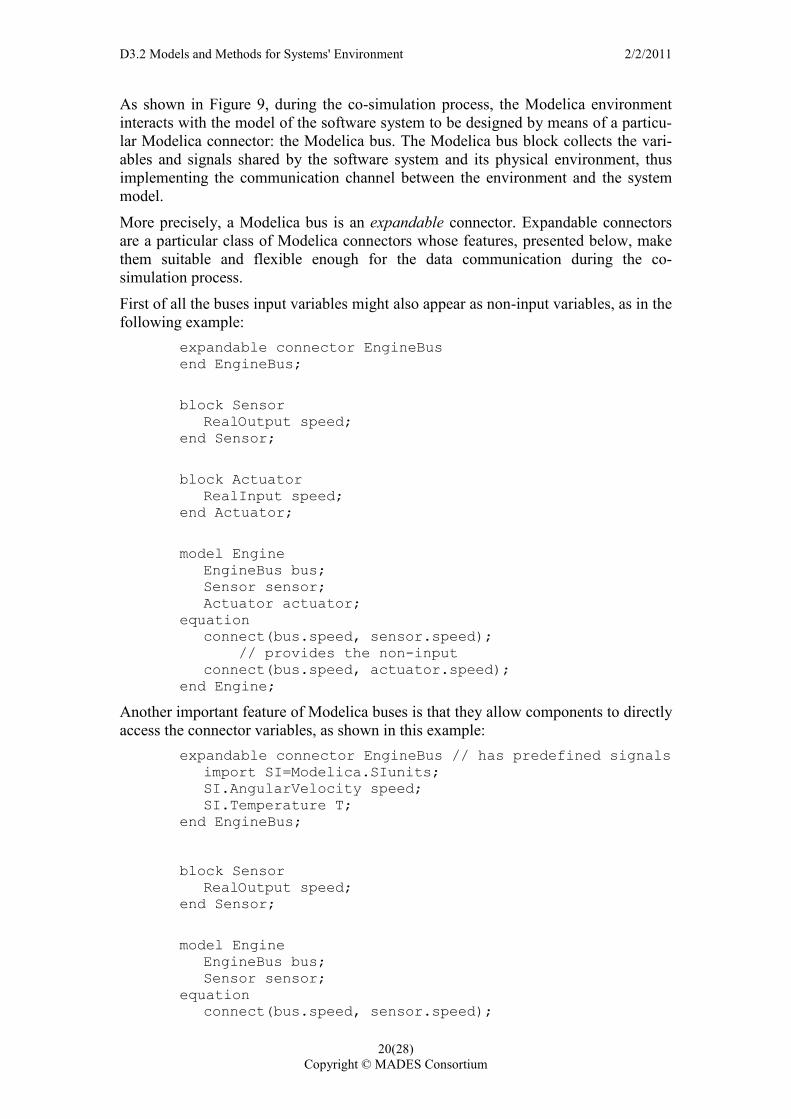
First of all the buses input variables might also appear as non-input variables, as in the following example:

expandable connector EngineBus end EngineBus;

block Sensor RealOutput speed; end Sensor;

block Actuator RealInput speed; end Actuator;

model Engine EngineBus bus; Sensor sensor; Actuator actuator; equation connect(bus.speed, sensor.speed); // provides the non-input connect(bus.speed, actuator.speed); end Engine;

Another important feature of Modelica buses is that they allow components to directly access the connector variables, as shown in this example:

expandable connector EngineBus // has predefined signals import SI=Modelica.SIunits; SI.AngularVelocity speed; SI.Temperature T; end EngineBus;

block Sensor RealOutput speed; end Sensor;

model Engine EngineBus bus; Sensor sensor; equation connect(bus.speed, sensor.speed);



// connection to non-connector speed is possible // in expandable connectors end Engine;

Finally, empty buses can be filled according to the specific needs:

expandable connector EmptyBus end EmptyBus;

model Controller EmptyBus bus1; EmptyBus bus2; RealInput speed; equation connect(speed, bus1.speed); // ok, only one undeclared // and it is unsubscripted connect(bus1.pressure, bus2.pressure); // not allowed, both undeclared connect(speed, bus2.speed[2]); // introduces speed array (with element [2]). end Controller;

Similarly to polymorphism, the instances of expandable connectors can be filled “at run time” through the connection statements. The EmptyBus instances within the Con-

troller model – bus1 and bus2 – shown above are filled with the speed variables.

Through expandable connectors it is possible to realize data communication during the co-simulation process in a suitably flexible manner.

In MADES simulation models, the Modelica Bus contains the information that is nec-essary for the model of the physical environment to interact with the software system. All the “boundary conditions”, thus the shared variables that constitute the interface between the software system being designed and its environment, appear in this com-ponent.

In the radar system introduced above, for example, the antenna subsystem (i.e., the environment) needs to know from the user interface certain information, such as, for example, the commands issued by the pilot. The user interface (i.e., the software sys-tem being designed) on the other hand, needs to know from the antenna subsystem some information about the state of the radar. All the information that is shared by the software system and its environment in MADES simulation models must be part of the Modelica bus; for example, the following declaration states that the data about the state of the radar is part of the bus:

expandable connector MadesBus import SI=Modelica.SIunits;

// ...

SI.Angle RadarStates[2]; end MadesBus;

To summarize, all variables that appear in the MadesBus model are shared by soft-ware system and environment. Some of these variables, e.g., the commands issued by the pilot in the radar example, are such that their values are determined by the soft-ware system and then read by the environment; other variables, e.g., the state of the radar, are such that their values are determined by the environment and then read by the software system.



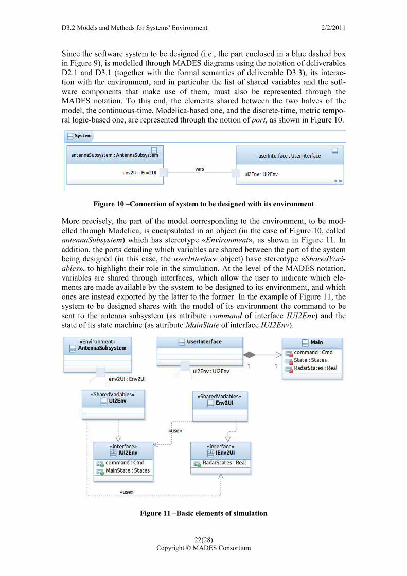
Since the software system to be designed (i.e., the part enclosed in a blue dashed box in Figure 9), is modelled through MADES diagrams using the notation of deliverables D2.1 and D3.1 (together with the formal semantics of deliverable D3.3), its interac-tion with the environment, and in particular the list of shared variables and the soft-ware components that make use of them, must also be represented through the MADES notation. To this end, the elements shared between the two halves of the model, the continuous-time, Modelica-based one, and the discrete-time, metric tempo-ral logic-based one, are represented through the notion of port, as shown in Figure 10.

Figure 10 –Connection of system to be designed with its environment

More precisely, the part of the model corresponding to the environment, to be mod-elled through Modelica, is encapsulated in an object (in the case of Figure 10, called antennaSubsystem) which has stereotype «Environment», as shown in Figure 11. In addition, the ports detailing which variables are shared between the part of the system being designed (in this case, the userInterface object) have stereotype «SharedVari-ables», to highlight their role in the simulation. At the level of the MADES notation, variables are shared through interfaces, which allow the user to indicate which ele-ments are made available by the system to be designed to its environment, and which ones are instead exported by the latter to the former. In the example of Figure 11, the system to be designed shares with the model of its environment the command to be sent to the antenna subsystem (as attribute command of interface IUI2Env) and the state of its state machine (as attribute MainState of interface IUI2Env).

Figure 11 –Basic elements of simulation



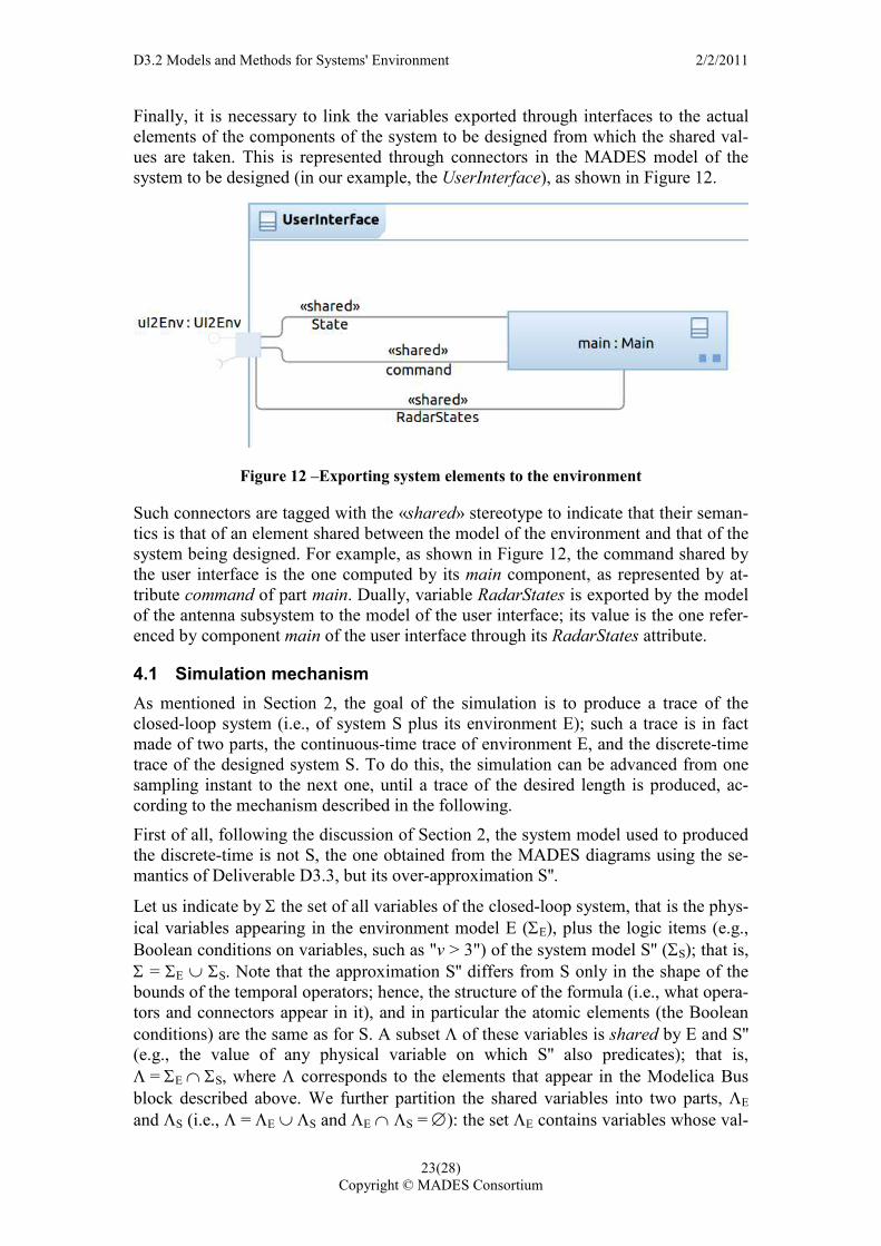
Finally, it is necessary to link the variables exported through interfaces to the actual elements of the components of the system to be designed from which the shared val-ues are taken. This is represented through connectors in the MADES model of the system to be designed (in our example, the UserInterface), as shown in Figure 12.

Figure 12 –Exporting system elements to the environment

Such connectors are tagged with the «shared» stereotype to indicate that their seman-tics is that of an element shared between the model of the environment and that of the system being designed. For example, as shown in Figure 12, the command shared by the user interface is the one computed by its main component, as represented by at-tribute command of part main. Dually, variable RadarStates is exported by the model of the antenna subsystem to the model of the user interface; its value is the one refer-enced by component main of the user interface through its RadarStates attribute.

4.1 Simulation mechanism

As mentioned in Section 2, the goal of the simulation is to produce a trace of the closed-loop system (i.e., of system S plus its environment E); such a trace is in fact made of two parts, the continuous-time trace of environment E, and the discrete-time trace of the designed system S. To do this, the simulation can be advanced from one sampling instant to the next one, until a trace of the desired length is produced, ac-cording to the mechanism described in the following.

First of all, following the discussion of Section 2, the system model used to produced the discrete-time is not S, the one obtained from the MADES diagrams using the se-mantics of Deliverable D3.3, but its over-approximation S''.

Let us indicate by Σ the set of all variables of the closed-loop system, that is the phys-ical variables appearing in the environment model E (ΣE), plus the logic items (e.g., Boolean conditions on variables, such as "v > 3") of the system model S'' (ΣS); that is, Σ = ΣE ∪ ΣS. Note that the approximation S'' differs from S only in the shape of the bounds of the temporal operators; hence, the structure of the formula (i.e., what opera-tors and connectors appear in it), and in particular the atomic elements (the Boolean conditions) are the same as for S. A subset Λ of these variables is shared by E and S'' (e.g., the value of any physical variable on which S'' also predicates); that is, Λ = ΣE ∩ ΣS, where Λ corresponds to the elements that appear in the Modelica Bus block described above. We further partition the shared variables into two parts, ΛE and ΛS (i.e., Λ = ΛE ∪ ΛS and ΛE ∩ ΛS = ∅): the set ΛE contains variables whose val-



ues are computed through the environment model E, which are "read" by the system model S'' (i.e., variables that are output by E to S); the set ΛS contains variables that are computed by the system model S'' and read by E (i.e., variables that are input to E from S). We call state σ of the closed-loop model a mapping from variables to their values: σ : Σ → DΣ, with DΣ the domains of the variables of the system; then, σ(v), with v ∈ Σ, is the value of variable v in state σ; also, if ∆ is a set included in, i.e., ∆ ⊆ Σ, σ(∆) is the set of values taken in state σ by the variables in set ∆.

The Modelica model is intrinsically deterministic, given an initial condition (i.e., from a given initial condition, there is only one trace that can be produced), while the met-ric temporal logic model S (and its approximation S'') is typically nondeterministic, as it represents all possible traces of the system being designed.

This suggests the following two-step mechanism for the advancement of the simula-tion from the current state σi to the state σi+1 in the next sampling instant.

1. From the values σi(ΣE), using the Modelica intepreter, compute σi+1(ΣE \ ΛS), i.e., the part of the new state that is "controlled" by the environment. Also, in this step the Modelica interpreter must check that Boolean conditions on the physical variables (e.g., "v > 3") that appear in S'' satisfy the non-berkeleyness constraint. If the trace produced by the Modelica interpreter is not non-berkeley, then it cannot be considered a suitable trace, since it cannot be guar-anteed that it satisfies S using the approach of Section 2.

2. Check, using a satisfiability checker for metric temporal logic formulae, such as Zot18, whether there exists a discrete-time trace of S'' that has ⟨σ0(Σ),σ1(Σ),...σi(Σ),σi+1(ΣE \ ΛS)⟩ as prefix; if there is, complete state σi+1 us-ing the part σi+1(ΣS \ ΛE) computed by Zot, and repeat from step 1.

If, however, it is not possible to complete the prefix ⟨σ0(Σ),σ1(Σ),...σi(Σ),σi+1(ΣE \ ΛS)⟩, then the simulation needs to backtrack to σi-1(Σ), and repeat from step 1, but feeding Zot suitable constraints to avoid producing again the same state σi(Σ) that led to the dead-end (for example, in Zot it is possible to specify a constraint such as " the system shall not be in state σi(Σ) after i instants").

To conclude this section, let us note that the approximation Ωδ of Figure 7 could be used to check whether a prefix π=⟨σ0(Σ),σ1(Σ),...σi(Σ)⟩ can indeed be completed to a trace of length k > i: if approximation Ωδ(S), with the constraint that the first i instants of the trace are equal to π, is not satisfiable, then so is the original model S. Hence, trying to complete prefix π using the two-step mechanism outlined above is useless, as it will never provide a suitable trace. This test can be used, for example, to weed out prefixes that, after a few tries, keep leading to dead-ends. If, however, Ωδ(S), with the additional constraint that π is a prefix of the trace, is satisfiable, due to the nature of the approximation it could still be the case that prefix π cannot be completed to a trace of desired length k: in other words, approximation Ωδ(S) can provide a definitive only if it is not satisfiable.

18 http://home.dei.polimi.it/pradella/Zot



5 Example

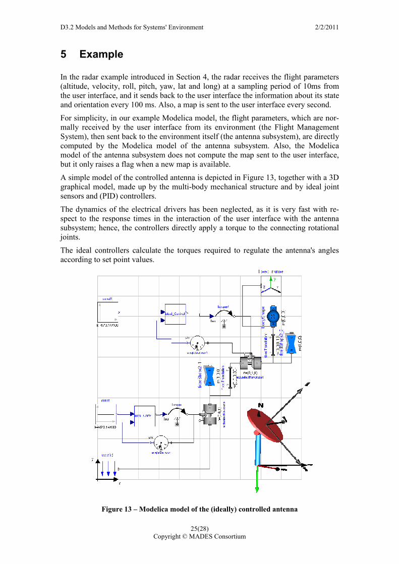
In the radar example introduced in Section 4, the radar receives the flight parameters (altitude, velocity, roll, pitch, yaw, lat and long) at a sampling period of 10ms from the user interface, and it sends back to the user interface the information about its state and orientation every 100 ms. Also, a map is sent to the user interface every second.

For simplicity, in our example Modelica model, the flight parameters, which are nor-mally received by the user interface from its environment (the Flight Management System), then sent back to the environment itself (the antenna subsystem), are directly computed by the Modelica model of the antenna subsystem. Also, the Modelica model of the antenna subsystem does not compute the map sent to the user interface, but it only raises a flag when a new map is available.

A simple model of the controlled antenna is depicted in Figure 13, together with a 3D graphical model, made up by the multi-body mechanical structure and by ideal joint sensors and (PID) controllers.

The dynamics of the electrical drivers has been neglected, as it is very fast with re-spect to the response times in the interaction of the user interface with the antenna subsystem; hence, the controllers directly apply a torque to the connecting rotational joints.

The ideal controllers calculate the torques required to regulate the antenna's angles according to set point values.

Figure 13 – Modelica model of the (ideally) controlled antenna



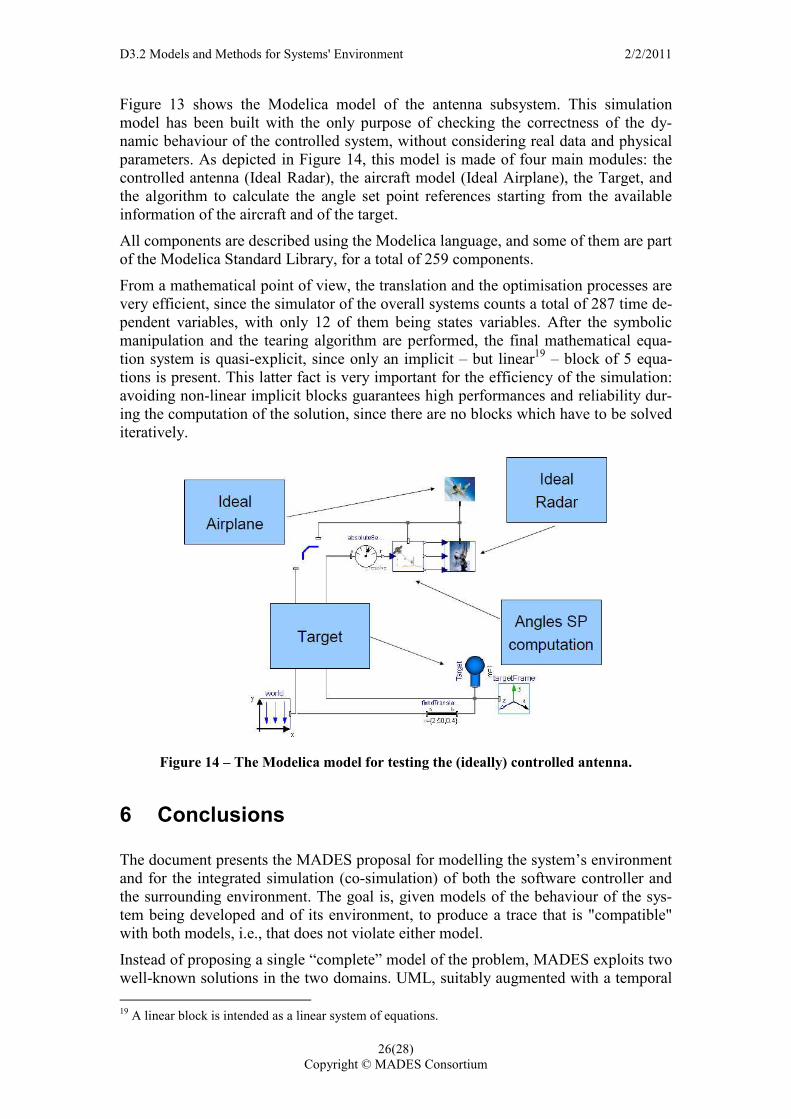
Figure 13 shows the Modelica model of the antenna subsystem. This simulation model has been built with the only purpose of checking the correctness of the dy-namic behaviour of the controlled system, without considering real data and physical parameters. As depicted in Figure 14, this model is made of four main modules: the controlled antenna (Ideal Radar), the aircraft model (Ideal Airplane), the Target, and the algorithm to calculate the angle set point references starting from the available information of the aircraft and of the target.

All components are described using the Modelica language, and some of them are part of the Modelica Standard Library, for a total of 259 components.

From a mathematical point of view, the translation and the optimisation processes are very efficient, since the simulator of the overall systems counts a total of 287 time de-pendent variables, with only 12 of them being states variables. After the symbolic manipulation and the tearing algorithm are performed, the final mathematical equa-tion system is quasi-explicit, since only an implicit – but linear19 – block of 5 equa-tions is present. This latter fact is very important for the efficiency of the simulation: avoiding non-linear implicit blocks guarantees high performances and reliability dur-ing the computation of the solution, since there are no blocks which have to be solved iteratively.

Figure 14 – The Modelica model for testing the (ideally) controlled antenna.

6 Conclusions

The document presents the MADES proposal for modelling the system’s environment and for the integrated simulation (co-simulation) of both the software controller and the surrounding environment. The goal is, given models of the behaviour of the sys-tem being developed and of its environment, to produce a trace that is "compatible" with both models, i.e., that does not violate either model.

Instead of proposing a single “complete” model of the problem, MADES exploits two well-known solutions in the two domains. UML, suitably augmented with a temporal 19 A linear block is intended as a linear system of equations.



logic semantics, for the definition of the software components and Modelica, along with its eco-system, for the environment. The result can be seen as a lightweight solu-tion where users can combine different complementary formalisms (differential equa-tions, logic formalisms) and expertise in a seamless manner. In addition, much of the complexity of producing the actual formal models is hidden: UML elements are as-cribed a formal semantics automatically, and the Modelica model can fully exploit the vast set of existing libraries.

This document introduces the theoretical and methodological solution and exemplifies it on a simple case study taken from the project’s demonstrators. Deliverable D3.5 will provide the actual integrated simulation environment and will also provide an empirical assessment of the main features of the proposal.

7 References

[BMMR10] L. Baresi, A. Morzenti, A. Motta and M. Rossi. 2010. From Interaction Overview Diagrams to Temporal Logic. In Proceedings of the 3rd International Workshop on Model Based Architecting and Construction of Embedded Systems (ACES-MB). 37-51.

[FR06] C. A. Furia, and M. Rossi. 2006. Integrating discrete- and continuous-time metric temporal logics through sampling. In Proceedings of the 4th International Con-ference on Formal Modelling and Analysis of Timed Systems (FORMATS). E. Asa-rin and P. Bouyer, Eds. Lecture Notes in Computer Science, vol. 4202. Springer-Verlag, Berlin, Germany, 215–229.

[FR08] C. A. Furia, and M. Rossi. 2008. MTL with bounded variability: Decidability and complexity. In Proceedings of the 6th International Conference on Formal Model-ling and Analysis of Timed Systems (FORMATS). F. Cassez and C. Jard, Eds. Lec-ture Notes in Computer Science, vol. 5215. Springer-Verlag, Berlin, Germany, 109–123.

[FR10] C. A. Furia and M. Rossi. 2010. A theory of sampling for continuous-time metric temporal logic. ACM Trans. Comput. Logic 12, 1, Article 8 (November 2010), 40 pages. http://doi.acm.org/10.1145/1838552.1838560.

[DL08] F. Donida, A. Leva. 2010. Modelica as a host language for process/control cosimulation and codesign. In Proceedings of the 2008 Modelica Conference, 3-4 March, Bielefeld, Germany, 401-408.

[GGJZ00] C. A. Gunter, E. L. Gunter, M. A. Jackson, and P. Zave: “A Reference Model for Requirements and Specifications”. IEEE Software 17(3):37-43, 2000.

[KTBL06] Simulation of complex systems using Modelica and tool coupling. In Pro-ceedings of the 2006 Modelica Conference, 4-5 September, Vienna, Austria, 485-490.

[MA93] Mattsson, S.E., Andersson, M. 1993. Omola – An Object-Oriented Modeling Language, Recent Advances in Computer Aided Control Systems. Elsevier Science, 291–310.

[MG98] Maffezzoni, C., Girelli, R. 1998. MOSES: Modular modeling of physical systems in an object-oriented database. Mathematical Modeling of Systems 4(2), 121–147.



[OP96] Oh, M., Pantelides, C.C. 1996. A modeling and simulation language for com-bined lumped and distributed parameter systems. Computers and Chemical Engineer-ing 20, 611–633.

[OW08] Ouaknine, J. and Worrell, J. 2008. Some Recent Results in Metric Temporal Logic, Formal Modeling and Analysis of Timed Systems, Lecture Notes in Computer Science, F. Cassez and C. Jard eds, , volume 5215, pp. 1-13, doi:10.1007/978-3-540-85778-5_1

[PEWW91] Piela, P.C., Epperly, T.G.,Westerberg, K.M.,Westerberg, A.W. 1991.ASCEND: An Object-Oriented Computer Environment for modelling and anal-ysis: the modelling language. Computers and Chemical Engineering 15(1), 53–72.

[HB97] K. Hines, G. Borriello Dynamic Communication Models in Embedded Sys-tem Co-Simulation, Design Automation Conference, 34th Conference on (DAC'97) Anaheim, CA, ISBN: 0-89791-920-3.

Documents

MADES-248864-D3.2 - Models and methods for systems environment v1api.ning.com/files/*MVnc9iSFPecGVS1rteaKUtxK1... · 2017-05-27 · D3.2 Models and Methods for Systems' Environment