Embed Size (px)
Citation preview

Groups and Representations
Madeleine Whybrow
Imperial College London
These notes are based on the course “Groups and Representations” taught
by Prof. A.A. Ivanov at Imperial College London during the Autumn term
of 2015.
Contents
1 Linear Groups 3
1.1 Finite Fields . . . . . . . . . . . . . . . . . . . . . . . . . . . . . . . . 3
1.2 Key Groups . . . . . . . . . . . . . . . . . . . . . . . . . . . . . . . . 4
1.2.1 The General Linear Group . . . . . . . . . . . . . . . . . . . 4
1.2.2 The Projective General Linear Group . . . . . . . . . . . . 5
1.2.3 The Special Linear Group . . . . . . . . . . . . . . . . . . . 5
1.2.4 The Projective Special Linear Group . . . . . . . . . . . . 5
1.3 A Simple Group of Order 60 . . . . . . . . . . . . . . . . . . . . . . 6
1.4 A Simple Group of Order 168 . . . . . . . . . . . . . . . . . . . . . 8
1.4.1 The Fano Plane . . . . . . . . . . . . . . . . . . . . . . . . . 8
1.4.2 The Automorphism Group of the Projective Plane . . . . 12
2 Stabilisers of Subgroups in GL(V ) 18
2.1 Semidirect Products . . . . . . . . . . . . . . . . . . . . . . . . . . . 18
2.2 General Theory of Stabilisers . . . . . . . . . . . . . . . . . . . . . . 21
1

3 The Representation Theory of L3(2) 22
3.1 Representation Theory . . . . . . . . . . . . . . . . . . . . . . . . . 22
3.1.1 The Dual of a Vector Space . . . . . . . . . . . . . . . . . . 24
3.1.2 Counting Irreducible Representations . . . . . . . . . . . . 25
3.2 Permutation Representations . . . . . . . . . . . . . . . . . . . . . . 25
3.2.1 Submodules of Permuation Modules . . . . . . . . . . . . . 26
3.2.2 Permutation Modules of 2-Transitive Actions . . . . . . . 27
3.2.3 Permutation Modules of Actions on Cosets of Subgroups 28
3.3 Representations of L3(2) over GF (2) . . . . . . . . . . . . . . . . . 30
3.3.1 The Permutation Module 2Ω . . . . . . . . . . . . . . . . . 31
3.3.2 The Permutation Modules 2Λ and 2∆ . . . . . . . . . . . . 32
3.4 Representations of L3(2) over C . . . . . . . . . . . . . . . . . . . . 35
3.4.1 The Ordinary Character Table of L3(2) . . . . . . . . . . . 37
A Error Correcting Codes 42
2

Chapter 1
Linear Groups
In this chapter, we will introduce some specific examples of linear groups.
1.1 Finite Fields
We first recall some key results concerning finite fields.
Theorem 1.1. Let p be a prime number and m be a positive integer. Then
there exists a unique (up to isomorphism) field of order q ∶= pm. We call it
GF (q).
If m = 1 in the above theorem then GF (p) ≅ Z/pZ.
For m > 1, choose f(x) to be an irreducible polynomial of degree m in GF (p)[x]
then we can construct GF (q) as
GF (q) ≅ GF (p)[x]/f(x)GF (p)[x].
This construction is independant of the choice of f(x). It relies on the fact
(which we will not prove) that such a polynomial exists for all p and m.
Example 1.2. We will construct GF (4). We have GF (2) = Z/2Z = 0,1. Take
3

f(x) = x2 + x + 1 then
GF (4) = 0,1, x, x + 1.
Note that (GF (q)∗,×) is isomorphic to the cyclic group of order q − 1.
We denote by Vn(q) the n-dimensional vector space over GF (q).
1.2 Key Groups
Recall that we define the centre of a group G as
Z(G) ∶= z ∈ G ∶ zg = gz∀g ∈ G
and that we define the commutator subgroup as
G′∶= ⟨[g, h] ∶ g, h ∈ G⟩
where [g, h] = g−1h−1gh. Equivalently, the commutator subgroup can be defined
as the minimal subgroup H such that G/H is abelian.
1.2.1 The General Linear Group
We define
GLn(q) ∶= the set of non-singular n × n matrices over GF (q)
∶= the set of linear bijections of from Vn(q) to itself.
It is possible to show that these two definitions are equivalent by choosing a
basis of Vn(q).
The order of GLn(q) is
∣GLn(q)∣ = qn(n−1)
2
n
∏i=1
(qi − 1).
If we let G = GLn(q) then
Z(G) = λIn ∶ λ ∈ GF (q)∗
4

and
G′= A ∶ det(A) = 1.
Note that the map det ∶ GLn(q)→ GF (q)∗ is a homomorphism.
1.2.2 The Projective General Linear Group
We define
PGLn(q) ∶= GLn(q)/Z(GLn(q)).
Then
∣PGLn(q)∣ =∣GLn(q)∣
q − 1.
1.2.3 The Special Linear Group
We note that the map det ∶ GLn(q)→ GF (q)∗ is a homomorphism and define
SLn(q) ∶= ker(det).
Then SLn(q)◁GLn(q) and
GLn(q)
SLn(q)≅ GF (q)×
so
∣SLn(q)∣ =∣GLn(q)∣
q − 1.
1.2.4 The Projective Special Linear Group
We define
PSLn(q) ∶= SLn(q)/Z(GLn(q))∩SLn(q).
Then
∣PSLn(q)∣ =∣SLn(q)∣
(n, q − 1)
where (n, q − 1) denotes the highest common factor of n and q − 1.
We also denote PSLn(q) as Ln(q).
In the tables below we calculate the value of ∣L2(q)∣ for some small values of q.
5
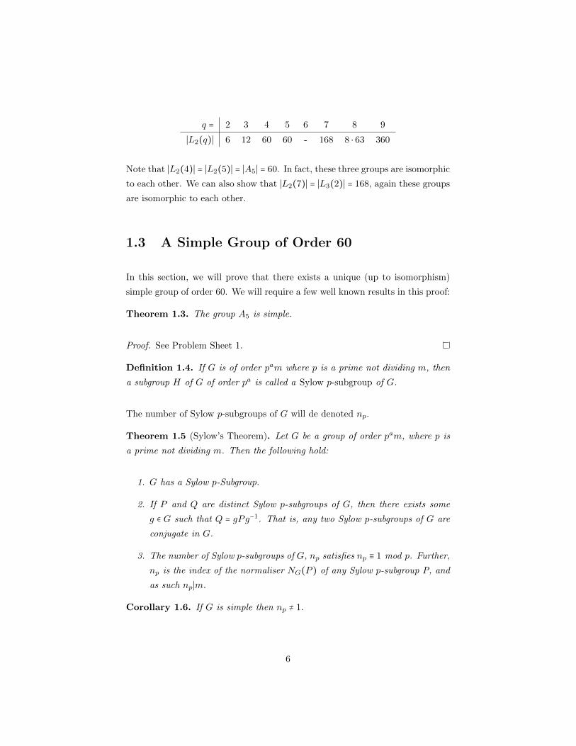
q = 2 3 4 5 6 7 8 9
∣L2(q)∣ 6 12 60 60 - 168 8 ⋅ 63 360
Note that ∣L2(4)∣ = ∣L2(5)∣ = ∣A5∣ = 60. In fact, these three groups are isomorphic
to each other. We can also show that ∣L2(7)∣ = ∣L3(2)∣ = 168, again these groups
are isomorphic to each other.
1.3 A Simple Group of Order 60
In this section, we will prove that there exists a unique (up to isomorphism)
simple group of order 60. We will require a few well known results in this proof:
Theorem 1.3. The group A5 is simple.
Proof. See Problem Sheet 1.
Definition 1.4. If G is of order pam where p is a prime not dividing m, then
a subgroup H of G of order pa is called a Sylow p-subgroup of G.
The number of Sylow p-subgroups of G will de denoted np.
Theorem 1.5 (Sylow’s Theorem). Let G be a group of order pam, where p is
a prime not dividing m. Then the following hold:
1. G has a Sylow p-Subgroup.
2. If P and Q are distinct Sylow p-subgroups of G, then there exists some
g ∈ G such that Q = gPg−1. That is, any two Sylow p-subgroups of G are
conjugate in G.
3. The number of Sylow p-subgroups of G, np satisfies np ≡ 1 mod p. Further,
np is the index of the normaliser NG(P ) of any Sylow p-subgroup P, and
as such np∣m.
Corollary 1.6. If G is simple then np ≠ 1.
6

Proof. Follows from the fact that any two Sylow p-subgroups are conjugate in
G.
Theorem 1.7. Suppose that H is a simple group of order 60. Then H ≅ A5.
Proof. Suppose that H is simple of order 60 = 22 ⋅3 ⋅5. Then by Sylow’s Theorem
n2 = 1,3,5 or 15;
n3 = 1,4 or 10;
n5 = 1 or 6.
As H is simple, Corollary 1.6 implies that n5 = 6. Let
K ∶= K(1)5 ,K
(2)5 ,K
(3)5 ,K
(4)5 ,K
(5)5 ,K
(6)5
be the set of Sylow 5-subgroups and let M = Sym(K) ≅ S6. Then we have a
map φ ∶H →M induced by the action of conjugation of H on K. We can show
that φ is a homomorphism and that φ(h) is a bijection for all h ∈H.
As H is simple, the kernel of φ must be trivial (as it is a normal subgroup of H
and φ is non-trivial). Thus H embeds into S6. Moreover, φ(H) ≤ Alt(K) ≅ A6,
otherwise φ(H) ∩Alt(K) would be an index 2 subgroup in φ(H) ≅ H which is
a contradiction as index 2 subgroups are necessarily normal.
We consider the action of Alt(K) on the cosets of φ(H). This gives a homo-
morphism
µ ∶ Alt(K)→ Sym(L) ≅ S6
where L is the set of cosets of φ(H) in Alt(K).
However, by comparing orders, we see that µ is actually an isomorphism Alt(K)→
Alt(L). Moreover, φ(H) as a subgroup of Alt(K) is the stabiliser of the coset
φ(H).1 so is isomorphic to a copy of A5 in Alt(L). Thus we have that H ≅ A5
is the only simple group of order 60.
7

1.4 A Simple Group of Order 168
In this section, we will prove that there exists a unique (up to isomorphism)
simple group of order 168.
1.4.1 The Fano Plane
We consider the group L3(2) = PSL3(2) = SL3(2) = GL2(3) = PGL3(2). It is
the automorphism group of V3(2). Note that for any vector space over a finite
field
∑v∈V
v = 0.
In fact, for any subspace U of V
∑v∈U
v = 0.
For any v ∈ V , scalar multiplication is easy to determine as 0v = 0 and 1v = v.
In order to determine addition in V3(2), we consider its two dimensional sub-
spaces. The number of two dimensional subspaces is
[3
2]2=
(23 − 1)(23 − 2)
(22 − 1)(22 − 2)= 7
where [nk]q
is defined to be the number of k-dimensional subspaces in Vn(q) and
is equal to
[n
k]q=
(qn − 1)(qn − q) . . . (qn − qk−1)
(qk − 1)(qk − q) . . . (qk − qk−1).
Each such subspace U contains three non-zero vectors, say U = 0, u1, u2, u3.
Thus, using the fact that ∑v∈U v = 0, we can define u1 + u2 to be u3, the third
non-zero vector in the 2-dimensional subspace containing u1 and u2.
Using this observation, we can express the two dimensional subspaces of V3(2)
as the Fano plane (the projective plane of order 2).
8

⎛
⎜⎜
⎝
1
1
1
⎞
⎟⎟
⎠
⎛
⎜⎜
⎝
1
0
1
⎞
⎟⎟
⎠
⎛
⎜⎜
⎝
1
0
0
⎞
⎟⎟
⎠
⎛
⎜⎜
⎝
1
1
0
⎞
⎟⎟
⎠
⎛
⎜⎜
⎝
0
1
0
⎞
⎟⎟
⎠⎛
⎜⎜
⎝
0
1
1
⎞
⎟⎟
⎠
⎛
⎜⎜
⎝
0
0
1
⎞
⎟⎟
⎠
Here, the points correspond to the vectors in V and the lines correspond to the
2-dimensional subspaces of V . We denote the set of points as P and the set
of lines L . A point in P lies on a line in L if and only if the corresponding
vector is contained in the corresponding 2-dimensional vector space. This gives
a set of incidence relations, which we denote I .
We can then define the Fano plane to be the triple Π ∶= (P,L ,I ). In fact
any plane can be described in this form, with sets of points and lines and
corresponding incidence relations.
If Π ∶= (P,L ,I ) and Π′ ∶= (P ′,L ′,I ′) are two planes then a map ψ ∶ Π→ Π′
is a morphism of planes if it maps points to points, lines to lines and p ∈ l if and
only if ψ(p) ∈ ψ(l) for and p ∈ P and l ∈ L .
The incidence relations I can be equivalently described using an incidence
matrix defined as
M(Π) ∶= (alp)l∈L ,p∈P
9

where
alp =
⎧⎪⎪⎪⎨⎪⎪⎪⎩
1 if p ∈ l
0 if p ∉ l.
For Π this gives the matrix below. The last row gives the vectors of V which
each of the columns refer to.
p1 p2 p3 p4 p5 p6 p7
l1 0 1 1 0 1 0 0
l2 0 0 1 1 0 1 0
l3 0 0 0 1 1 0 1
l4 1 0 0 0 1 1 0
l5 0 1 0 0 0 1 1
l6 1 0 1 0 0 0 1
l7 1 1 0 1 0 0 0
⎛⎜⎜⎜⎝
1
0
0
⎞⎟⎟⎟⎠
⎛⎜⎜⎜⎝
0
1
0
⎞⎟⎟⎟⎠
⎛⎜⎜⎜⎝
0
0
1
⎞⎟⎟⎟⎠
⎛⎜⎜⎜⎝
1
1
0
⎞⎟⎟⎟⎠
⎛⎜⎜⎜⎝
0
1
1
⎞⎟⎟⎟⎠
⎛⎜⎜⎜⎝
1
1
1
⎞⎟⎟⎟⎠
⎛⎜⎜⎜⎝
1
0
1
⎞⎟⎟⎟⎠
Note that the matrix above obeys the following rules:
A1 There are 7 rows;
A2 There are 7 columns;
A3 There are 3 ones in each row;
A4 There are 3 ones in each column;
A5 The inner product of two distinct rows is 1;
A6 The inner product of two distinct columns is 1;
where the inner product of two rows or columns is their inner product as vectors
i.e. coordinate-wise multiplication. We will now show that these rules are in
fact sufficient to describe the Fano plane.
Proposition 1.8. A plane whose incidence matrix obeys the axioms A1 - A6
is unique up to isomorphism.
10

Sketch of proof. Any plane is isomorphic to another plane whose incidence ma-
trix has its ones as far upwards and leftwards as possible (as an isomorphism of
a plane is effectively a relabelling of its points and lines).
There is only one matrix in this form which obeys the axioms above, we call it
M . Thus a plane whose incidence matrix obeys the rules above is isomorphic
to the plane whose incidence matrix is equal to M .
M =
p1 p2 p3 p4 p5 p6 p7
l1 1 1 1 0 0 0 0
l2 1 0 0 1 1 0 0
l3 1 0 0 0 0 1 1
l4 0 1 0 0 1 0 0
l5 0 1 0 0 1 0 1
l6 0 0 1 1 0 0 1
l7 0 0 1 0 1 1 0
There is yet another equivalent way in which we can consider the Fano plane.
We now take P = GF (7), Q ∶= α2 ∶ α ∈ GF (7) = 1,2,4 and L = Q+ i ∶ i ∈
GF (7). Note that the set Q is a difference set.
Proposition 1.9. The plane with points and lines described above is the Fano
plane.
Proof. Check that the incidence matrix obeys the axioms A1-A6.
Expressing elements of L as vectors in V7(2) where the ith coordinate of the
vector corresponding to l ∈ L is 1 if and only if pi ∈ l give vectors which all lie
in the Hamming code Ham(3) (see Appendix A).
If we include the zero vector we can extend our matrix to get
11

⎛⎜⎜⎜⎝
0
0
0
⎞⎟⎟⎟⎠
⎛⎜⎜⎜⎝
1
0
0
⎞⎟⎟⎟⎠
⎛⎜⎜⎜⎝
0
1
0
⎞⎟⎟⎟⎠
⎛⎜⎜⎜⎝
0
0
1
⎞⎟⎟⎟⎠
⎛⎜⎜⎜⎝
1
1
0
⎞⎟⎟⎟⎠
⎛⎜⎜⎜⎝
0
1
1
⎞⎟⎟⎟⎠
⎛⎜⎜⎜⎝
1
1
1
⎞⎟⎟⎟⎠
⎛⎜⎜⎜⎝
1
0
1
⎞⎟⎟⎟⎠
1 0 1 1 0 1 0 0
1 0 0 1 1 0 1 0
1 0 0 0 1 1 0 1
1 1 0 0 0 1 1 0
1 0 1 0 0 0 1 1
1 1 0 1 0 0 0 1
1 1 1 0 1 0 0 0
0 1 0 0 1 0 1 1
0 1 1 0 0 1 0 1
0 1 1 1 0 0 1 0
0 0 1 1 1 0 0 1
0 1 0 1 1 1 0 0
0 0 1 0 1 1 1 0
0 0 0 1 0 1 1 1
.
This matrix is of the form
N =
⎡⎢⎢⎢⎢⎣
1 M
0 M ′
⎤⎥⎥⎥⎥⎦
where M is the incidence matrix of (P,L ) and M ′ is its complement.
The rows of this matrix, along with the vectors 1 and 0 give a Hamming Code
Ham(3) which has been extended by a parity check bit.
As usual, the columns of N correspond to vectors V ∶= V3(2) and the rows
correspond to U + v where U is a fixed 2-dimensional subspace of V and v ∉ U .
1.4.2 The Automorphism Group of the Projective Plane
If Π = (P,L ) is the Fano plane, recall that
Aut(Π) = φ ∶ P →P a bijection such that φ(l) ∈ L ∀l ∈ L .
12
Labelling the points as p1, . . . , p7 means we can write such automorphisms as
elements of S7.
Example 1.10.
φ = (1)(2 4)(3 5)(7 6) ∉ Aut(Π)
φ = (1)(2 4)(3 5)(7)(6) ∈ Aut(Π)
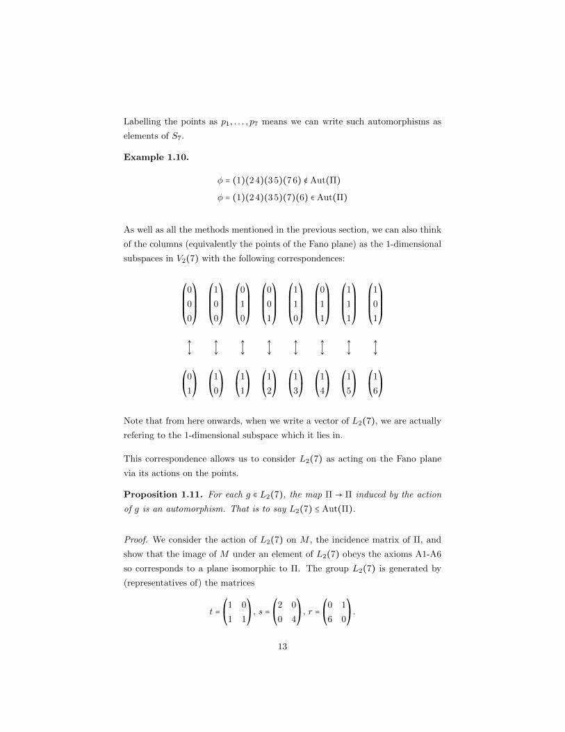
As well as all the methods mentioned in the previous section, we can also think
of the columns (equivalently the points of the Fano plane) as the 1-dimensional
subspaces in V2(7) with the following correspondences:
⎛⎜⎜⎜⎝
0
0
0
⎞⎟⎟⎟⎠
⎛⎜⎜⎜⎝
1
0
0
⎞⎟⎟⎟⎠
⎛⎜⎜⎜⎝
0
1
0
⎞⎟⎟⎟⎠
⎛⎜⎜⎜⎝
0
0
1
⎞⎟⎟⎟⎠
⎛⎜⎜⎜⎝
1
1
0
⎞⎟⎟⎟⎠
⎛⎜⎜⎜⎝
0
1
1
⎞⎟⎟⎟⎠
⎛⎜⎜⎜⎝
1
1
1
⎞⎟⎟⎟⎠
⎛⎜⎜⎜⎝
1
0
1
⎞⎟⎟⎟⎠
Õ×Ö
Õ×Ö
Õ×Ö
Õ×Ö
Õ×Ö
Õ×Ö
Õ×Ö
Õ×Ö
⎛
⎝
0
1
⎞
⎠
⎛
⎝
1
0
⎞
⎠
⎛
⎝
1
1
⎞
⎠
⎛
⎝
1
2
⎞
⎠
⎛
⎝
1
3
⎞
⎠
⎛
⎝
1
4
⎞
⎠
⎛
⎝
1
5
⎞
⎠
⎛
⎝
1
6
⎞
⎠
Note that from here onwards, when we write a vector of L2(7), we are actually
refering to the 1-dimensional subspace which it lies in.
This correspondence allows us to consider L2(7) as acting on the Fano plane
via its actions on the points.
Proposition 1.11. For each g ∈ L2(7), the map Π → Π induced by the action
of g is an automorphism. That is to say L2(7) ≤ Aut(Π).
Proof. We consider the action of L2(7) on M , the incidence matrix of Π, and
show that the image of M under an element of L2(7) obeys the axioms A1-A6
so corresponds to a plane isomorphic to Π. The group L2(7) is generated by
(representatives of) the matrices
t =⎛
⎝
1 0
1 1
⎞
⎠, s =
⎛
⎝
2 0
0 4
⎞
⎠, r =
⎛
⎝
0 1
6 0
⎞
⎠.
13
For α ∈ GF (7), the matrix t maps
⎛
⎝
1
α
⎞
⎠↦
⎛
⎝
1
α + 1
⎞
⎠.
Rows of M can also be thought of as subsets of the form l = 1 + i,2 + i,4 + i
for i ∈ GF (7). Thus t simply permutes the rows of M , and so the image of M
under t will obey the axioms, as required.
Similarly, the matrix s maps
⎛
⎝
1
α
⎞
⎠↦
⎛
⎝
2
4α
⎞
⎠=⎛
⎝
1
2α
⎞
⎠.
So will map l = 1 + i,2 + i,4 + i to 2 + 2i,4 + 2i,8 + 2i ≡ 1 + 2i,2 + 2i,4 + 2i.
So similarly s permutes the rows of M .
The case of r is not so straightforward. It sends maps
⎛
⎝
1
α
⎞
⎠↦
⎛
⎝
α
6α
⎞
⎠.
Check by hand that this maps
⎛
⎝
1
0
⎞
⎠↦
⎛
⎝
1
0
⎞
⎠,⎛
⎝
1
1
⎞
⎠↦
⎛
⎝
1
6
⎞
⎠,⎛
⎝
1
2
⎞
⎠↦
⎛
⎝
2
6
⎞
⎠=⎛
⎝
1
3
⎞
⎠,⎛
⎝
1
3
⎞
⎠↦
⎛
⎝
3
6
⎞
⎠=⎛
⎝
1
2
⎞
⎠
⎛
⎝
1
4
⎞
⎠↦
⎛
⎝
4
6
⎞
⎠=⎛
⎝
1
5
⎞
⎠,⎛
⎝
1
5
⎞
⎠↦
⎛
⎝
5
6
⎞
⎠=⎛
⎝
1
4
⎞
⎠,⎛
⎝
1
6
⎞
⎠↦
⎛
⎝
6
6
⎞
⎠=⎛
⎝
1
1
⎞
⎠
and that the image of the matrix M under this map obeys axioms A1-A6 so is
still an incidence matrix of the Fano plane.
Theorem 1.12. The Fano plane is uniquely determined by the choice of three
non-collinear points.
Proof. Suppose that we choose u, v,w three non-collinear points in Π. In the
Fano plane, any two points lie in a unique line so the points u + v, u +w, v +w
complete the three lines containing pairs of u, v and w. As u, v,w are non-
collinear, these points are distinct. However, the points u + v, u + w, v + w are
clearly collinear, give us a fourth line. The point u+ v +w is again distinct and
so the lines u, v + w,u + v + w, v, u + w,u + v + w amd w,u + v, u + v + w
complete the Fano plane, as required.
14

Proposition 1.13. ∣Aut(Π)∣ ≤ 168
Proof. From Theorem 1.12 above, an automorphism of Π is determined by its
action on any three non-collinear points of the Fano plane. Fix three such points.
Then there are 7 choices for the image of the first point, 6 for the second and 4
for the third. Thus there are at most 168 automorphisms of Π.
Theorem 1.14. L2(7) ≅ Aut(Π)
Proof. From Proposition 1.11 and Proposition ?? we know that L2(7) ≤ Aut(Π)
and ∣Aut(Π)∣ ≤ 168. However, ∣L3(2)∣ = 168 so we must have L3(2) ≅ Aut(Π).
Any element l of L clearly acts on U . Recall that we have a map
β ∶ [U
1]→ V
sending
⎛
⎝
0
1
⎞
⎠
⎛
⎝
1
0
⎞
⎠
⎛
⎝
1
1
⎞
⎠
⎛
⎝
1
2
⎞
⎠
⎛
⎝
1
3
⎞
⎠
⎛
⎝
1
4
⎞
⎠
⎛
⎝
1
5
⎞
⎠
⎛
⎝
1
6
⎞
⎠
⎛⎜⎜⎜⎝
0
0
0
⎞⎟⎟⎟⎠
⎛⎜⎜⎜⎝
1
0
0
⎞⎟⎟⎟⎠
⎛⎜⎜⎜⎝
0
1
0
⎞⎟⎟⎟⎠
⎛⎜⎜⎜⎝
0
0
1
⎞⎟⎟⎟⎠
⎛⎜⎜⎜⎝
1
1
0
⎞⎟⎟⎟⎠
⎛⎜⎜⎜⎝
0
1
1
⎞⎟⎟⎟⎠
⎛⎜⎜⎜⎝
1
1
1
⎞⎟⎟⎟⎠
⎛⎜⎜⎜⎝
1
0
1
⎞⎟⎟⎟⎠
.
We can use this to define an action of l on V . We say that
vl = β((β−1(v))l)
giving the commutative diagram
v β−1(v)
vl (β−1(v))l
l
β−1
l
β.
15
We define
λ(l) = t0l ⋅ l
where tv ∶ u↦ u + v for u, v ∈ V . Then λ is our desired isomorphism.
Example 1.15. Take
l =⎛
⎝
1 1
0 1
⎞
⎠∈ GL2(7)
and let l be its representative in L2(7). Then l maps
∞ 0 1 2 3 4 5 6
⎛
⎝
0
1
⎞
⎠
⎛
⎝
1
0
⎞
⎠
⎛
⎝
1
1
⎞
⎠
⎛
⎝
1
2
⎞
⎠
⎛
⎝
1
3
⎞
⎠
⎛
⎝
1
4
⎞
⎠
⎛
⎝
1
5
⎞
⎠
⎛
⎝
1
6
⎞
⎠
l
⎛
⎝
1
1
⎞
⎠
⎛
⎝
1
0
⎞
⎠
⎛
⎝
1
4
⎞
⎠
⎛
⎝
1
3
⎞
⎠
⎛
⎝
1
6
⎞
⎠
⎛
⎝
1
5
⎞
⎠
⎛
⎝
1
2
⎞
⎠
⎛
⎝
0
1
⎞
⎠
So we can write l as a permutation
l = (∞1 4 5 2 3 6).
We have
0 = β⎛⎜⎝
⎛
⎝
0
1
⎞
⎠
l⎞⎟⎠= β
⎛
⎝
⎛
⎝
1
1
⎞
⎠
⎞
⎠=
⎛⎜⎜⎜⎝
0
1
0
⎞⎟⎟⎟⎠
.
Writing t0l as a permutation of elements of V gives
t0l =
⎛⎜⎜⎜⎝
⎛⎜⎜⎜⎝
0
0
0
⎞⎟⎟⎟⎠
⎛⎜⎜⎜⎝
0
1
0
⎞⎟⎟⎟⎠
⎞⎟⎟⎟⎠
⎛⎜⎜⎜⎝
⎛⎜⎜⎜⎝
1
0
0
⎞⎟⎟⎟⎠
⎛⎜⎜⎜⎝
1
1
0
⎞⎟⎟⎟⎠
⎞⎟⎟⎟⎠
⎛⎜⎜⎜⎝
⎛⎜⎜⎜⎝
0
0
1
⎞⎟⎟⎟⎠
⎛⎜⎜⎜⎝
0
1
1
⎞⎟⎟⎟⎠
⎞⎟⎟⎟⎠
⎛⎜⎜⎜⎝
⎛⎜⎜⎜⎝
1
1
1
⎞⎟⎟⎟⎠
⎛⎜⎜⎜⎝
1
0
1
⎞⎟⎟⎟⎠
⎞⎟⎟⎟⎠
(∞1) (0 3) (2 4) (5 6).
So
λ(l) = t0l ⋅ l = (∞) (1 2 0 3 5 4 6).
Using the basis (1,0,0)⊺, (0,1,0)⊺, (0,0,1)⊺, we can write λ(l) as the linear
transformation
λ(l) =
⎛⎜⎜⎜⎝
1 0 1
1 0 0
0 1 0
⎞⎟⎟⎟⎠
.
16

Using this isomorphism and Theorem 1.14 we have
L3(2) ≅ L2(7) ≅ Aut(Π).
17

Chapter 2
Stabilisers of Subgroups in
GL(V )
In this section we will consider a vector space V and a subspace U of V . Our
aim is to determine
G(U) ∶= StabGL(V )(U) = g ∈ GL(V ) ∶ Ug = U.
2.1 Semidirect Products
For a group G with a normal subgroup N ⊴ G, we have the quotient
G/N ∶= Ng ∶ g ∈ G.
Given a pair (N,G/N) up to isomorphism, is it possible to reconstruct G? In
general, this is a very hard, but important, question to answer. Semidirect
products are a special case of this problem where, given certain information
about N and G/N, it is possible to reconstruct G.
Example 2.1. If N ≅ C2 and G/N ≅ C2 then G may be equal to C4 or C2 ×C2.
18
Suppose that N ⊴ G and K ≤ G. Then we have a map
φ ∶ G→ G/N
g ↦ Ng.
When is φ∣K ∶K → K/K∩N an isomorphism?
• The kernel of φ∣K is K ∩N so φ∣K is injective if and only if K ∩N = 1;
• We will have Im(φ∣K) = Im(φ) if and only if ∀g ∈ G, ∃k ∈ K such that
Ng = Nk. So φ∣K is surjective if and only if G =KN ∶= ⟨kn ∶ k ∈K,n ∈ N⟩.
Definition 2.2. Given G a group with N ⊴ G and K ≤ G such that K ∩N = 1
and G = KN then G is said to be an internal semidirect product of N and K
(denoted G = N ⋊K).
As N is normal, we can take
λ ∶K → Aut(N)
k ↦ (n↦ k−1nk).
Thus, given the triple (N,K,λ), we can recover the group G = N ⋊ K. In
general, given any two groups K and H and a homomorphism λ ∶K → Aut(N),
we define the outer semidirect product of N and K with respect to λ to be the
set
N ⋊λK ∶= (k,n) ∶ k ∈K, n ∈ N.
with multiplication
(k1, n1) ⋅ (k2, n2) = (k1k2, nλ(k1)
1 n2).
Theorem 2.3. The set N ⋊λK as defined above is a group.
Note that if λ is the identity map then N ⋊λK ≅ N ×K.
Example 2.4 (The Stabiliser of the Extended Hamming Code). Let H be the
extended Hamming code of degree 3 (which we first saw on page 12). It is a
19

subspace of V8(2) and has parity-check matrix
H =
⎛⎜⎜⎜⎜⎜⎜⎝
0 1 0 0 1 0 1 1
0 0 1 0 1 1 0 1
0 0 0 1 0 1 1 1
1 1 1 1 1 1 1 1
⎞⎟⎟⎟⎟⎟⎟⎠
.
So the group GL4(2) acts on the Hamming code via its action on the columns
of this matrix. However, this action may not necessarily preserve the Hamming
code, but might send it to a different subspace of V8(2). This action will preserve
the code if and only if it permutes the columns of H.
Using the basis e1, e2, e3, e4 of V ∶= V4(2), the columns of H form the following
set
X = α1e1 + . . . + α4e4 ∣α4 = 1.
This is not a subspace of V but the set
Y = α1e1 + . . . + α4e4 ∣α4 = 0.
is a subspace. Moreover, V is the disjoint union of X and Y so the stabiliser of
X in GL(V ) is equal to the stabiliser of Y in GL(V ).
Thus the stabiliser consists of matrices which preserve the final basis vector of
V and which acts as GL3(2) on the remaining basis vectors.
Thus the stabiliser of the Hamming code in G = GL4(2) is
GH =
⎧⎪⎪⎪⎪⎪⎪⎪⎪⎨⎪⎪⎪⎪⎪⎪⎪⎪⎩
⎛⎜⎜⎜⎜⎜⎜⎝
0
A 0
0
x y z 1
⎞⎟⎟⎟⎟⎟⎟⎠
∶ A ∈ GL3(2), x, y, z ∈ GF (2)
⎫⎪⎪⎪⎪⎪⎪⎪⎪⎬⎪⎪⎪⎪⎪⎪⎪⎪⎭
= N ⋊λK
where N ≅ C32 , K ≅ GL3(2) and λ is the natural action of GL3(2) on V3(2).
Note that the action of the subgroup L isomorphic to GL3(2) in this stabiliser
preserves the first column of the parity check matrix, which corresponds to the
first bit, or column, of the extended Hamming code itself. However we know that
K ≅ L2(7) also acts on the columns of H via its action on the 1-dimensional
subspaces of V2(7). It is clear that this action stabilises H but does not preserve
any columns. Thus L and K are not conjugate in GH but are isomorphic.
20

To have two non-conjugate copies of Ln(2) in 2n ⋊Ln(2) is unique to the case
n = 3, it does not occur for any larger n.
2.2 General Theory of Stabilisers
The above example is a specific case of the general theory of stabilisers which
we will cover in this section.
Given a vector space V = Vn(q) and a subspace U of V , we wish to find the
stabiliser of the U which is defined as
G(U) ∶= g ∈ G ∶ Ug = U
for G = GL(V ) ≅ GLn(q).
Take B = b1, . . . , bn be a basis of V and let U = Span(b1, . . . , bm) for some
m ≤ n.
Then we have
G(U) =
⎧⎪⎪⎨⎪⎪⎩
⎛
⎝
X 0
P Y
⎞
⎠∶ X ∈ GL(U), Y ∈ GL(W ), P ∈Mn−m,m(q)
⎫⎪⎪⎬⎪⎪⎭
where W = Span(bm+1, . . . , bn) and Mn−m,m(q) is the set of matrices with n−m
rows and m columns over GF (q). This gives
∣G(U)∣ = ∣GLm(q)∣ ⋅ ∣GLn−m(q)∣ ⋅ qm(n−m).
It can also be deduced that
∣GL(V )∣ = ∣GL(U)∣ ⋅ [n
m]q.
Thus we have that
G(U) ≅ P ⋊λK
where
• K = Gm(q) ×Gn−m(q) corresponding to the matrices X and Y ;
• P = (Cq)(n−m)m corresponding to (n −m)m copies of the additive group
of GF (q).
21

Chapter 3
The Representation Theory
of L3(2)
In this chapter we will construct a number of representations of the group
G = L3(2). We will be working both with fields of characteristic 0 (ordinary
representation theory) and fields of positive characteristic (modular representa-
tion theory). We assume a basic knowledge of ordinary representation theory
but spend the next two sections going over results which will be particularly
key to our work.
3.1 Representation Theory
Recall that given two modules V1 and V2 of a group G along with representations
ϕ1 ∶ G → GL(V1) and ϕ2 ∶ G → GL(V2), we define the direct sum of V1 and V2
to be
V1 ⊕ V2 ∶= (v1, v2) ∶ v1 ∈ V1, v2 ∈ V2
with representation ϕ = ϕ1 ⊕ ϕ2 such that
ϕ ∶ (v1, v2)↦ (ϕ1(g)v1, ϕ2(v2)).
22

If there exist submodules V1 and V2 of V such that V = V1 ∪ V2 and V1 ∩ V2 = 0
then V = V1 ⊕ V2.
Our main strategy for constructing representations of L3(2) will be to construct
a permuation module V (see below) of G and then to (attempt to) decompose
it into the direct sum
V = V1 ⊕ . . .⊕ Vk (3.1)
where V1, . . . , Vk are irreducible representations.
In such a decomposition, the same submodule of V may occur more than once (or
indeed not at all). Given a module V and a submodule U (which not necessarily
irreducible) we say that the number of times U occurs as a decomposition factor
of V is the multiplicity of U in V and is denoted mV (U). For ease of notation,
if it is obvious to which module V we are referring, we write m(U).
From this discussion, the equation 3.1 becomes
V =l
⊕i=1
V ⊕mii = V1 . . . V1
´¹¹¹¹¹¹¹¹¹¹¹¹¹¸¹¹¹¹¹¹¹¹¹¹¹¹¶m1 times
⊕ . . .⊕ Vl . . . Vl´¹¹¹¹¹¹¹¹¹¹¸¹¹¹¹¹¹¹¹¹¹¶ml times
where the Vi are pair-wise non-isomorphic irreducible representations of G and
mi ∶=mV (Vi).
Proposition 3.1. If V is any module of a finite group and U is an irreducible
module of the same group then
mV (U) = ⟨χV , χU ⟩
where ⟨ , ⟩ is the inner product on characters of G.
Proof. We decompose V as
V = U⊕m(U)⊕
W ∈Irr(G)
W≠U
Wm(W ).
We then take the inner product of both sides with U to get
⟨χV , χU ⟩ =m(U)⟨χU , χU ⟩ ∑χW ∈Irr(G)
W≠U
⟨χW , χU ⟩.
23

However, recall that the irreducible representations are orthonormal with re-
spect to ⟨ , ⟩ so
⟨χW , χU ⟩ =
⎧⎪⎪⎪⎨⎪⎪⎪⎩
1 if W = U
0 if W ≠ U.
Thus
mV (U) = ⟨χV , χU ⟩.
However, such a decomposition is not always possible. If a module V can be
completely decomposed as a direct sum of irreducible modules then we say it is
semisimple.
Theorem 3.2 (Maschke’s Theorem). Let V be a module of a finite group G
over a field of characteristic p. Then V is semisimple if p does not divide the
order of G.
If a module V is not semisimple then it is possible that it contains two submod-
ules V1, V2 of a module such that V /V1 ≅ V2 but V /≅ V1 ⊕ V2. In this case, we
say that V is an indecomposable extension of V1 by V2 which we denote
V = V1/V2.
3.1.1 The Dual of a Vector Space
We will frequently use the following definition in this section.
Definition 3.3. If V is a vector space over the field k then the dual space of
V is
V ∗∶= Homk(V, k).
Example 3.4. What is the dual space of Vn(k) for a given field k? Given two
vectors v,w ∈ Vn(k), their dot product lies in k. So, for a given vector v ∈ Vn(k),
we can define a function
ϕv ∶ w ↦ v ⋅w.
It is clear that ϕv ∈ (Vn(k))∗. In fact, the map v ↦ ϕv induces an isomorphism
Vn(k) ≅ (Vn(k))∗.
24

3.1.2 Counting Irreducible Representations
We know that the number of ordinary representations of a group G is equal
to the number of conjugacy classes of G. There is an analogue for modular
representation theory:
Theorem 3.5. The number of irreducible representations of a group G over a
field of characteristic p is equal to the number of conjugacy classes of G whose
elements have order coprime to p.
Example 3.6. The group L3(2) has four conjugacy classes with elements of
odd order; the class consisting of the identity element, the class with elements
of order 3 and the two classes with elements of order 7. Thus L3(2) has four
irreducible representations over fields of characteristic 2.
3.2 Permutation Representations
Given a group G of permuations of a set Ω (i.e. a group which acts on a set),
permutation representations give a very easy way of constructing representa-
tions of G. Although permutation representations are not in general irreducible,
decomposing them may give a good way of constructing some irreducible rep-
resentations.
Given a finite field GF (q), we construct the permutation representation of G
over Ω as the vector space whose basis is indexed by the elements of Ω. That is
to say
V ∶= ∑ω∈Ω
α(ω)ω ∶ α(ω) ∈ GF (q).
We can equivalently think of this as
GF (q)Ω= qΩ
∶= f ∶ Ω→ GF (q)
the set of functions from Ω to GF (q). Given an element ∑ω∈Ω α(ω)ω of V , the
map ω ↦ α(ω) uniquely determines an element of GF (q)Ω and vice versa.
The group G acts on V and GF (q)Ω via its action on Ω. That is to say we have
25

a map G→ GL(V ) which sends g to
λ(g) ∶ ∑ω∈Ω
α(ω)ω ↦ ∑ω∈Ω
α(ω)ωg
f ↦ (fg ∶ ω ↦ ωg−1
).
Example 3.7. The group S5 has a 5-dimensional permutation over GF (2) with
basis vectors e1, e2, e3, e4, e5. Choose g = (1 2 3)(4 5) and v = (1,0,1,1,0) then
g ∶ v ↦ (1,1,0,0,1)
by permuting the basis vectors of V .
Lemma 3.8. The map g ↦ λ(g) is a representation (i.e. a homomorphism) of
G into GL(V ).
In practise, we consider λ(g) as acting on the basis vectors of V , then extend
this action linearly. The vector space V ≅ qΩ is called the GF (q) permutation
module of G acting on Ω.
Proposition 3.9. If χ ∶ G→ k is the character of the permutation module of G
acting on a set X then for any g ∈ G
χ(g) = ∣x ∈X ∶ gx = x∣.
That is to say, the value of a permuation character on an element g ∈ G is equal
to the number of fixed points of g.
3.2.1 Submodules of Permuation Modules
As usual, we say that a subspace U of V is a submodule if the map G→ GL(U)
which send g ↦ λ(g)∣U is also a representation. We wish to study the submodule
structure of permutation modules.
To begin with, there are two obvious submodules which lie inside any permuta-
tion module:
V (1)∶ = ∑α(ω)ω ∶ α(ω) = α(δ) for some fixed δ ∈ Ω
= the constant functions Ω→ GF (q)
V (n−1)∶ = ∑α(ω)ω ∶ ∑α(ω) = 0 .
26

So V (1) is a 1-dimensional submodule and V (n−1) is a (n − 1)-dimensional sub-
module.
Note that V (1) ⊆ V (n−1) if and only if ∑ω∈Ω 1 = 0 = n i.e. if and only if p∣n where
q = pm for some m ∈ N. We say that
V (n−1)/V (1)∩V (n−1)
is the heart of the representation.
Theorem 3.10. If G = Sym(Ω) then the heart of the representation qΩ is
irreducible.
3.2.2 Permutation Modules of 2-Transitive Actions
Definition 3.11. Suppose that G is a group acting on a set Ω. Then we say
that the action of G on Ω is transitive if for all x, y ∈ Ω, there exists g ∈ G such
that gx = y.
Moreover, for an integer n ≤ ∣Ω∣, we say that this action is n-transitive if for all
subsets x1, . . . , xn and y1, . . . , yn of Ω such that the xi and yi are pairwise
distinct, there exists g ∈ G such that gxi = yi for 1 ≤ i ≤ n.
Proposition 3.12. A group G acts 2-transitively on a set Ω if and only if it
has exactly two orbits on Ω ×Ω. They are
• (α,α) ∶ α ∈ Ω;
• (α,β) ∶ α,β ∈ Ω, α ≠ β.
Lemma 3.13 (Burnside’s Lemma). Let G be a finite group acting on a set X
then1
∣G∣∑g∈G
∣x ∈X ∶ gx = x∣ = # orbits of G on X.
This can of course be reformulated as
1
∣G∣∑g∈G
χ(g) = # orbits of G on X.
where χ is the character of the permutation module of the action of G on X.
27

Proposition 3.14. If a group G acts on a set Ω then the permutation module
over a field k of G acting on Ω decomposes as
kΩ= 1⊕ V
where 1 is the trivial module and V ∈ Irr(G), V ≠ 1.
Proof. Suppose that
kΩ=
n
⊕i=1
V ⊕mii
where Vi ∈ Irr(G). Suppose that χ is the character of V and χi is the character
of Vi for 1 ≤ i ≤ n. Then
⟨χ,χ⟩ =n
∑i=1
m2i .
However, we also have
⟨χ,χ⟩ = ⟨χ × χ,1G⟩
where χ × χ is the permutation character of the action of G on Ω ×Ω. Thus
⟨χ,χ⟩ =1
∣G∣∑g∈G
(χ × χ)(g)
= # orbits of G on Ω ×Ω = 2.
So the only possibilities for the values of the mi is that m1 =m2 = 1 and mi = 0
for i ≠ 1,2. One of the modules V1, V2 must be the trivial module and the other
an irreducible module of dimension ∣Ω∣ − 1.
3.2.3 Permutation Modules of Actions on Cosets of Sub-
groups
Proposition 3.15. Suppose that G is a finite group with H ≤ G. Let Ω ∶= G/H
and let V = kΩ, the permutation module of G acting on Ω via right multiplication
of cosets. Then for any irreducible submodule U of V ,
mV (U) = dimCU(H)
where
CU(H) ∶= v ∈ U ∶ hv = v∀h ∈H.
28

Proof. Using Propositions 3.1 and 3.9, we calculate
⟨χV , χU ⟩G =1
∣G∣∑g∈G
χV (g−1)χU(g) =
1
∣G∣∑g∈G
∑ω∈Ωgω=ω
χU(g)
=1
∣G∣∑ω∈Ω
∑g∈Ggω=ω
χU(g) =1
∣G∣∑ω∈Ω
∑G(ω)
χU(g)
=1
∣G∣∑ω∈Ω
∑h∈H
χU(h) =1
∣H ∣∑h∈H
χU(h)
= ⟨χU ,1H⟩H =m1
where m1 is the multiplicity of the trivial module in U .
Conversely, v ∈ V is contained in CU(H) if any only if the module ⟨v⟨ is isomor-
phic to the trivial module. Thus
CU(H) = ⊕m1
i=1Vi
where Vi is isomorphic to the trivial module for 1 ≤ i ≤m1. Thus
dimCU(H) =m1
as required.
Corollary 3.16. Suppose that V1, . . . , Vn are the irreducible representations of
a group G. Suppose also that for 1 ≤ i ≤ n, di ∶= dim(Vi). Then
∣G∣ =n
∑i=1
d2i .
Proof. We consider the action of G on itself by left multiplication (the regular
action of G) and denotes its corresponding permuation module by kG. This can
be equivalently thought of as the action of G on cosets of the trivial subgroup.
So, for any V ∈ Irr(G),
mkG(V ) = dim(CkG(e)) = dim(V ).
So if V1, . . . , Vn are representatives of the isomorphism classes of the irreducible
modules of G then
kG =n
⊕i=1
V⊕dim(Vi)i .
29

Now let χG be the character of kG. By the orthonormality of irreducible char-
acters we have
⟨χG, χG⟩ =n
∑i=1
(dim(Vi))2.
For g ∈ G
χG(g) =
⎧⎪⎪⎪⎨⎪⎪⎪⎩
∣G∣ if g = e
0 if g ≠ e.
So
⟨χG, χG⟩ =1
∣G∣∑g∈G
χG(g−1)χG(g) = ∣G∣
as required.
Corollary 3.17. A group G is abelian if and only if every irreducible represen-
tation is linear (1 dimensional).
Proof. Let n be the number of conjugacy classes of G. Then G is abelian if
and only if n = ∣G∣, with each class containing just one element. From Corollary
3.16,
∣G∣ =n
∑i=1
d2i .
and di ≥ 1 for 1 ≤ i ≤ n. Thus n = ∣G∣ if and only if di = 1 for 1 ≤ i ≤ n.
3.3 Representations of L3(2) over GF (2)
First, note that any permutation representation over GF (2) of a group G via
its action on Ω can be equivalently be thought of as the set of subsets of Ω i.e.
A ∶ A ⊆ Ω.
This correspondence can be formalised by associating with each subset A ⊂ Ω
the vector ∑α(ω)ω where α(ω) = 1 if and only if ω ∈ A.
We now return to the specific case of G = L3(2). We will consider the following
three permuation modules:
30

1. 2Ω - the 7-dimensional permutation module based on the action of L3(2)
on Ω = V3(2)/0;
2. 2∆ - the 8-dimensional permutation module based on the action of L2(7)
on the 1-dimensional subspaces of V2(7);
3. 2Λ - the 24-dimensional permutation module based on the action of L3(2)
on Λ ∶= G/S via right multiplication of cosets where S is a Sylow 7-
subgroup of L3(2).
We have already extensively studied the first two actions when looking at the
Fano plane but this is the first time that we have seen the action of G on Λ.
Our aim is to decompose these permutation modules into direct sums of the
irreducible representations of G over GF (2). From Theorem 3.5, we know that
there are four such representations.
Note that 2 divides the order of G so these modules are not necessarily semisim-
ple but there is still a fair amount that we can say about their internal structure.
3.3.1 The Permutation Module 2Ω
As per our initial discussion on general permutation modules, 2Ω has the sub-
modules V (1) and V (6). Moreover, since ∣Ω∣ = 7 is odd, these two submodules
are disjoint and so we have
2Ω= V (6)
⊕ V (1).
In fact, the module V (6) has further structure
V (6)= V3(2)
∗/V3(2)
where / denotes an indecomposable extension of modules and V3(2)∗ is the dual
of V3(2). We can think of V3(2) and V3(2)∗ as
V3(2) =
⎧⎪⎪⎪⎪⎪⎨⎪⎪⎪⎪⎪⎩
⎛⎜⎜⎜⎝
a1
a2
a3
⎞⎟⎟⎟⎠
∶ a1, a2, a3 ∈ GF (2)
⎫⎪⎪⎪⎪⎪⎬⎪⎪⎪⎪⎪⎭
V3(2)∗= (b1 b2 b3) ∶ b1, b2, b3 ∈ GF (2) .
31

Moreover, it turns out that V3(2) and V3(2)∗ are two of the irreducible modules
of G over GF (2).
We now have
2Ω= (V3(2)
∗/V3(2))⊕ 1.
However, this is not a direct sum decomposition of 2Ω as
V3(2)∗/V3(2) /≅ V3(2)
∗⊕ V3(2).
3.3.2 The Permutation Modules 2Λ and 2∆
We now consider the permutation modules 2Λ and 2∆. Our aim is to find the
submodule decomposition of 2Λ and to use this to show that the module contains
a copy of the Golay code.
We first note that 2∆ can equivalently be thought of as the permutation module
of G acting by conjugation on its 8 Sylow 7-subgroups.
Proposition 3.18. The permutation module 2∆ is a direct summand of 2Λ.
Proof. We will show that there exists a G-invariant surjective homomorphism
φ ∶ 2Λ → 2∆. Then ker(φ) will be a submodule of 2Λ such that 2Λ/ker(φ) ≅ 2∆.
First take λ ∈ Λ. Then we define
G(λ) = g ∈ G ∶ g(λ) = λ
so that G(λ) is a conjugate of S and so is also a Sylow 7-subgroup of G. Then
the map Λ→∆ sending λ↦ G(λ) extends to a surjective G-invariant surjective
homomorphism φ ∶ 2Λ → 2∆.
Theorem 3.19. Let H be a Sylow 2-subgroup in G and let V be a module of
G over GF (2). If U is a non-trivial submodule of V then H fixes at least one
non-zero vector in U .
Proof. If k is the dimension of U then
∣U/0∣ = 2k − 1.
32

As U is stable under the action of G (and therefore the action of any of its
subgroups) U is the union of H-orbits. Moreover every H-orbit has length 2ei
for some ei. Thus
2k − 1 =l
∑i=1
2ei
and so it follows that ei = 0 for some i. Then the corresponding orbit has length
one so consists of a non-zero vector which is stabilised by H.
We know that 2∆ is a submodule of 2Λ but how do we go about finding other
submodules?
Note that
V3(2)⊗ V3(2)∗=
⎧⎪⎪⎪⎪⎪⎨⎪⎪⎪⎪⎪⎩
⎛⎜⎜⎜⎝
u1v1 u1v2 u1v3
u2v1 u2v2 u2v3
u3v1 u3v2 u3v3
⎞⎟⎟⎟⎠
∶ u ∈ V3(2), v ∈ V3(2)∗
⎫⎪⎪⎪⎪⎪⎬⎪⎪⎪⎪⎪⎭
≅M3(2)
and that G ≅ GL3(2) acts on V3(2)⊗V3(2)∗ via conjugation of matrices, turning
it into a 9-dimensional module of G.
It is easy to spot that
V1 ∶=
⎧⎪⎪⎪⎪⎪⎨⎪⎪⎪⎪⎪⎩
⎛⎜⎜⎜⎝
0 0 0
0 0 0
0 0 0
⎞⎟⎟⎟⎠
,
⎛⎜⎜⎜⎝
1 0 0
0 1 0
0 0 1
⎞⎟⎟⎟⎠
⎫⎪⎪⎪⎪⎪⎬⎪⎪⎪⎪⎪⎭
is a submodule of V3(2)⊗ V3(2)∗. Its complement is
V8 ∶= M ∶ tr(M) = 0.
In fact this module V8 is know as the Steinberg module of L3(2) and is an
irreducible representation of G over GF (2).
Proposition 3.20.
2Λ= V
(1)8 ⊕ V
(2)8 ⊕ 2∆
where V(1)8 and V
(2)8 are copies of V8.
Proof. Consider S a Sylow 7-subgroup of G and suppose that S = ⟨s⟩ for some
element s ∈ G. Then the characteristic polynomial p(s) is irreducible, so either
p(s) = λ3+ λ + 1 or p(s) = λ3
+ λ2+ 1.
33

For any matrix, the coefficient of the second highest power in its characteristic
equation is equal to its trace. Thus if χ(s) is equal to the first polynomial, s is
traceless, else if it is equal to the second, it has trace 1.
Moreover, if λ3 + aλ2 + bλ + c is the characteristic polynomial of s, then s−1 has
characteristic polynomial cλ3 + bλ2 + aλ + 1. On the other hand, s and s2 have
the same characteristic polynomial.
It follows that there are exactly three elements of S whose corresponding ma-
trices are traceless and are thus contained in a copy of V8. Suppose without loss
of generality that s is traceless. Then s2 and s4 are too. Thus
CV8(S) = 0, s, s2, s4
and m2Λ(V8) = 2.
Now, by comparing dimensions, along with Proposition 3.18, we have
2Λ= V
(1)8 ⊕ V
(1)8 ⊕ 2∆.
as required.
Note that there are actually three copies of V8 in 2Λ, the third of which we
denote V(3)8 . If we index the basis vectors of V
(1)8 and V
(2)8 as v1, . . . , v8 and
u1, . . . , v8 then
V(3)8 = (vi, ui) ∶ 1 ≤ i ≤ 8.
Our next aim is to find an explicit basis of 2Λ in terms of the right hand side
of the equality proved in the previous result. We are trying to find a vector
vs ∈ V(1)8 ⊕ V
(2)8 ⊕ 2∆ such that
vgs ∶ g ∈ G
forms a basis of 2Λ.
Chose a non-zero vector in 2∆. Then this vector is a Sylow 7-subgroup, call it
S. Without loss of generality, we can assume that S = ⟨s⟩ where s is a traceless
matrix of order 7.
34

Now let s1 and s2 be the vectors corresponding to s in V(1)8 and V
(2)8 respectively.
We can take
vs = (s1, si2, S)
for i = 1,2 or 4. If i = 1 then (s1, s2) ∈ V(3)8 and vs ∈ V
(3)8 ⊕ 2∆. Thus i = 2 or 4.
Without loss of generality, we can take i = 2 and
vs = (s1, s22, ⟨s⟩).
Then
vs ∶ s ∈ V8, ∣⟨s⟩∣ = 7
is a basis for 2∆.
All that remains is to show that 2Λ contains a copy of the Golay code. Recall
that the elements of ∆ index the columns of the extended Hamming code. Thus
extended Hamming code is a submodule of 2∆ of dimension 4. Moreover, we
know that L2(7) is the automorphism group of H. However, PGL2(7) also acts
on H, and contains L2(7) as an index two subgroup.
Take an element α ∈ PGL2(7)/L2(7) e.g.
α =⎛
⎝
1 0
0 −1
⎞
⎠.
We can also write this as a permutation of the columns of H to get
α = (∞)(0)(1 6)(2 5)(3 4).
Check that Hα is an extended Hamming code which is L2(7)-invariant. More-
over Hα ≠ H because α ∉ Aut(H) and H +Hα is a submodule of 2∆ of codi-
mension 1 and H ∩Hα = 1.
As the Golay code is 12-dimensional, it must contain one of the three Steinberg
modules V(i)8 for i = 1,2,3 and one of the two 4-dimensional submodules of 2Λ,
H and Hα. In fact, all of these six different combinations of modules give us a
submodule isomorphic to the Golay code.
3.4 Representations of L3(2) over C
We start by deducing the dimensions of the irreducible representations.
35
The action of G ≅ L3(2) on the following sets is 2-transitive:
• ∆, the 1-dimensional subspaces of V2(7);
• P, the points of the Fano plane;
• L , the lines of the Fano plane.
So by Proposition 3.14, we have the following decompositions:
• C∆ = 1⊕ V7;
• CP = 1⊕ V(1)6 ;
• CL = 1⊕ V(2)6 ;
for V7, V(1)6 , V
(2)6 ∈ Irr(G). In fact,
V(1)6 ≅ V
(2)6 .
Now consider the action of L3(2) on the set of flags of the Fano plane:
θ = (p, l) ∶ p ∈ P, l ∈ L .
There are 21 incidence relations of the Fano plane so Cθ is a 21-dimensional
permutation module. It can be decomposed as
Cθ = 1⊕ V(1)6 ⊕ V
(2)6 ⊕ V8
where V8 is an 8-dimensional irreducible module of G.
When proving the simplicity and uniqueness of the simple group G of order 168
(which we now know to be L3(2)) we (implicitly) showed that G has 7 conjugacy
classes, which we denote1
1A,2A,3A,4A,7A,7B.
1The notation NX is a standard way of representing a conjugacy class. The integer N
refers to the order of the elements of the class. The smallest class with elements of order N
is labelled NA, the next largest NB and so on.
36

Thus
∣Irr(G)∣ = # conjugacy classes of G = 6.
We already have four irreducible representations, one each of dimensions 1, 6,
7 and 8. Let x and y denote the dimensions of the remaining two irreducible
representations. Then, from Corollary 3.16
12+ 62
+ 72+ 82
+ x2+ y2
= ∣G∣ = 168.
Thus we have
x2+ y2
= 18
and the only possibility is that x = y = 3 so that the final two irreducible
representations of G have dimension 3.
3.4.1 The Ordinary Character Table of L3(2)
We denote the irreducible representations of G as
V1, V(1)3 , V
(2)3 , V6, V7, V8.
Theorem 3.21. The character table of G ≅ L3(2) ≅ L7(2) is
1A 2A 3A 4A 7A 7B
1 21 56 42 24 24
χ1 1 1 1 1 1 1
χ(1)3 3 −1 0 1 b7 −b∗7
χ(2)3 3 −1 0 1 −b∗7 b7
χ6 6 2 0 0 −1 −1
χ7 7 −1 1 −1 0 0
χ8 8 0 −1 0 1 1
where the second row gives the sizes of the conjugacy classes, and
b7 ∶=1 +
√−7
2and b∗7 ∶=
1 −√−7
2.
Proof. Since we know the dimensions of the irreducible modules, we know the
value which their characters take at e, giving the first column. The trivial
character takes the value of one everywhere, giving the first row.
37

For the characters corresponding to the 6 and 8 dimensional representations, we
recall that
χCP = χCL = 1 + χ6
χCθ = 1 + 2χ6 + χ8.
and that the value of a permutation character at an element g ∈ G is the number
of fixed points of the permuation induced by g. Thus, for example, if g ∈ G then
χ6(g) is equal to the number of points (or lines) of the Fano plane fixed by g
minus 1.
An element of order 2 in G acts on the Fano plane by stabilising a line l and by
transposing the two points on each other line which do not also lie on l. Thus
if g ∈ 2A, then g fixes three points (those on l) and 5 flags so
χ6(g) = 3 − 1 = 2 and χ8(g) = 5 − 1 − 4 = 0.
An element of order 3 in G acts on the Fano plane by fixing one point and
acting as a cyclic permutation on the three lines which contain that point.
Thus if g ∈ 3A then g fixes one point and no flags so
χ6(g) = 1 − 1 = 0 and χ8(g) = 0 − 1 = −1.
An element of order 4 in G acts on the Fano plane by fixing one point, transpos-
ing two of the lines which is contained in and transposing the two other points
on the third line in which it lies. Thus if g ∈ 4A, then g fixes one line and one
flag (the fixed point and the line it is contained in which is not transposed with
another)
χ6(g) = 1 − 1 = 0 and χ8(g) = 1 − 1 = 0.
Finally, an element of order 7 in G acts cyclicly on the points and lines of the
Fano planes. Thus if g ∈ 7A or g ∈ 7B, then g fixes no points and no flags and
χ6(g) = 0 − 1 = −1 and χ8(g) = 0 − 1 + 2 = 1.
Let
t =⎛
⎝
1 0
1 1
⎞
⎠, s =
⎛
⎝
2 0
0 4
⎞
⎠, r =
⎛
⎝
0 1
6 0
⎞
⎠.
38

Then t is of order 2, s is of order 3 and r is of order 7. From the discussion
following Propostition 1.11, we know that
• t fixes none of the 1-dimensional subspaces of V2(7);
• s fixes two such subspaces, those generated by⎛
⎝
0
1
⎞
⎠and
⎛
⎝
1
0
⎞
⎠;
• r fixes one such subspace, that generated by⎛
⎝
0
1
⎞
⎠.
As characters are constant on conjugacy classes, these observations give us the
values of χ7 for the conjugacy classes 2A, 3A and 7A. The remaining two values
for χ7 can be deduced from the orthogonality of the rows of the character table.
We now turn our attention to the final two characters - those of dimension 3.
Take g to be an element of the 7A conjugacy class. Then the restriction of the
presentation to ⟨g⟩ will be the direct sum of three 1-dimensional representations
(see Corollary 3.17). Thus the matrices of the image of g under each of the two
3-dimensional representations are of the form
⎛⎜⎜⎜⎝
em1
7 0 0
0 em2
7 0
0 0 em3
7
⎞⎟⎟⎟⎠
for mi ∈ Z for 1 ≤ i ≤ 3 and where en ∶= e2πin .
Given an element h ∈ NL3(2)(⟨g⟩) and an irreducible representation ρ of ⟨g⟩ the
map
ρh ∶ x↦ ρ(xh)
is also an irreducible representation. Thus it follows that we have an action of
NL3(2)(⟨g⟩) on the irreducible characters of ⟨g⟩.
If h ∈ ⟨g⟩ then h acts trivially (as characters are constant on conjugacy classes).
If h ∈ NL3(2)(⟨g⟩)/⟨g⟩ then h induces a non-trivial permuation of the represen-
tations of ⟨g⟩. However, as h ∈ L3(2), the action it induces on the characters of
L3(2) must be trivial. Thus the action of NL3(2)(⟨g⟩) on the representations in
question must preserve the set m1,m2,m3.
39

In particular, NL3(2)(⟨g⟩) is generated by g and a 3-cycle h such that h−1gh = g2.
Thus the possibilities for m1,m2,m3 are 3,5,6 and 1,2,4 giving character
values of b7 and −b∗7 for χ(1)3 and χ
(2)3 respectively. The values of these characters
on 7B can be deduced from the orthogonality of the columns of the character
table.
Moreover, the automorphism ρ(1)3 (g) of V clearly has three distinct eigenvalues,
e7, e27 and e4
7 so we have a basis of V consisting of eigenvectors of ρ(1)3 (g). As
the element h permutes these eigenvectors, ρ(1)3 (g) will be a matrix conjugate
to⎛⎜⎜⎜⎝
0 0 1
1 0 0
0 1 0
⎞⎟⎟⎟⎠
.
This argument also holds for ρ(2)3 so we can conclude that the character values of
the two 3-dimensional representations are 0 on the conjugacy class of elements
of order 3.
We now claim that the image of L3(2) under either of the representations of di-
mension 3 is contained in SL3(C). Since L3(2) is simple and the representations
in question are not trivial, both have trivial kernels. Thus they give embeddings
of L3(2) into GL3(C). As SL3(C) is normal in GL3(C), the intersection of the
image of L3(2) and SL3(C) is normal in the image of L3(2) and so must either
be trivial, or must be the whole of the group.
The intersection cannot be trivial as we have already shown that an element of
order 7 in L3(2) is mapped to a matrix with determinant 1 in GL3(2). Thus
the image of L3(2) under the two representations of dimension 3 is contained
in SL3(C), as required.
Now consider an element x of order 2. By the same reasoning as in the case
of the 7A conjugacy class, the image of x under one of the representations of
dimension 3 the must be of the form
⎛⎜⎜⎜⎝
en1
2 0 0
0 en2
2 0
0 0 en1
2
⎞⎟⎟⎟⎠
for ni ∈ Z for 1 ≤ i ≤ 3. We must have (ni,2) = 1 for some 1 ≤ i ≤ 3, else the
40

representation would be trivial. Along with the fact that this matrix must have
determinant 1, this implies that the only possibility for n1, n2, n3 is 1,1,2.
Thus both characters of dimension 3 take the value -1 on the conjugacy class of
involutions.
Finally, we consider an element y of order 4. As before, the image of y under
either of the representations of dimension 3 must be of the form
⎛⎜⎜⎜⎝
ep1
4 0 0
0 ep4
4 0
0 0 ep1
4
⎞⎟⎟⎟⎠
for pi ∈ Z for 1 ≤ i ≤ 3. Moreover, we must have (pi,4) = 1 for at least one
1 ≤ i ≤ 3, else the matrix would be of order 1 or 2. In this case, NL3(2)(⟨y⟩)
is generated by y and z, an element of order 2 such that z−1yz = y3. Using
these observations, along with the fact that the image of y must be a matrix
of determinant 1, we deduce that the only possibility for p1, p2, p3 is 1,3,4.
Thus both characters of dimension 3 take the value 0 on the conjugacy class of
elements of order 4.
41
Appendix A
Error Correcting Codes
Definition A.1. A (binary) code of length n is a subset C of Vn(2). The
vectors in C are called codewords. The distance between two codewords x, y is
d(x, y), the number of coordinates where x and y differ in value.
Definition A.2. The minimum distance of a code C is
d(C) = mind(x, y) ∶ x, y ∈ C,x ≠ y.
Definition A.3. A code C is a linear code if it is a subspace of Vn(2).
The motivation for studying codes is that they offer a certain level of error
correction. Suppose we transmit a codeword c ∈ C but e errors are made and
we actually receive vector b ∉ C. Then, as long as e is sufficiently small, if we
send b to its nearest vector in C, this vector will be our original codeword c.
So we can think of each codeword as being a (binary) message which we want
to transmit, along with a certain number of bits of extra information which will
enable us to recover c if it is corrupted in transmission.
Formally, we say that a code C ⊂ Vn(2) corrects e errors if for any c, c′ ∈ C and
x ∈ Vn(2), if d(c, x) ≤ e and d(c′, x) ≤ e then c = c′.
Ideally, we are looking for codes which correct a high number of errors and have
low dimension and minimum distance.
42

Definition A.4. If A ∈Mn(2) and C = x ∈ Vn(2) ∶ Ax = 0 then C is a linear
code and A is said to be its check matrix.
Proposition A.5. Let C be a code with check matrix A. Suppose
1. all columns of A are different;
2. no column of A is the zero vector.
Then C corrects at least one error.
Proposition A.6. Let d ≥ 2 and let C be a linear code with check matrix A.
Assume that every set of d − 1 columns of A are linearly independent. Then
d(C) ≥ d
Definition A.7. Let k ≥ 2. A Hamming code Ham(k) is a code whose check
matrix has for columns all non-zero vectors in Vk(2).
A Hamming code Ham(k)
• has minimum distance 3;
• has length 2k − 1;
• has dimension 2k − k − 1;
• corrects one error.
It is a perfect code which (informally) means it corrects the highest possible
number of errors for a given dimension and minimum weight.
There are only three possible types of perfect codes, the Hamming codes which
corrects one error, the codes C = 0n,1n which correct n−12
errors and a third,
called the Golay code.
The Golay code is actually constructed from the Hamming code. We start with
a code H ∶= Ham(3) with check matrix
⎛⎜⎜⎜⎝
1 1 1 0 1 0 0
1 1 0 1 0 1 0
1 0 1 1 0 0 1
⎞⎟⎟⎟⎠
43

and it’s “reverse” K with check matrix
⎛⎜⎜⎜⎝
0 0 1 0 1 1 1
0 1 0 1 0 1 1
1 0 0 1 1 0 1
⎞⎟⎟⎟⎠
.
Then, to each codeword in H and K, we add a “parity check bit”. That is to
say, given a vector (v1, . . . , v7) we add an eighth bit
v8 =7
∑i=1
vi
which is 1 if there is an even number of 1’s and 0 if there are an odd number.
This gives us two codes H ′ and K ′ of length 8.
Definition A.8. The extended Golay code is defined as
G24 ∶= (a + x, b + x, a + b + x) ∶ a, b ∈H ′, x ∈K ′ ⊆ V24(2)
The Golay code G23 consists of the codewords of the extended Golay code with
the last bit removed.
The Golay code is perfect and
• has minimum length 7;
• has length 23;
• has dimension 12;
• corrects 3 errors.
44