Madagascar tutorial: Field data processing

Madagascar tutorial: Field data processing

Maurice the Aye-Aye

ABSTRACT

In this tutorial, you will learn about multiple attenuation using parabolic Radontransform (Hampson, 1986). You will first go through an example that explainsthe process step by step. You will be asked to change some parameters and addmissing few lines. In the next part of the tutorial, you will be asked to apply thesame workflow to another CMP gather. The CMP gathers used in the tutorialare from the Canterbury data set (Lu et al., 2003). By the end of this tutorial,you should have learned to:

1. apply NMO and inverse NMO for a CMP gather,

2. apply forward and inverse parabloic Radon transform,

3. design a mute function that preserves multiples in the Radon domain,

4. subtract multiples from the data,

5. create a semblance scan for a CMP gather.

PREREQUISITES

Completing this tutorial requires

• Madagascar software environment available fromhttp://www.ahay.org

• LATEX environment with SEGTeX available fromhttp://www.ahay.org/wiki/SEGTeX

To do the assignment on your personal computer, you need to install the requiredenvironments. An Internet connection is required for access to the data repository.

The tutorial itself is available from the Madagascar repository by running

svn co https://rsf.svn.sourceforge.net/svnroot/rsf/trunk/book/rsf/school2012

Madagascar Documentation

http://www.ahay.org

http://www.ahay.org/wiki/SEGTeX

Maurice 2 Tutorial

INTRODUCTION

In this tutorial, you will be asked to run commands from the Unix shell (identifiedby bash$) and to edit files in a text editor. Different editors are available in a typicalUnix environment (vi, emacs, nedit, etc.)

Your first assignment:

1. Open a Unix shell.

2. Change directory to the tutorial directory

bash$ cd $RSFSRC/book/rsf/school2012

3. Open the tutorial.tex file in your favorite editor, for example by running

bash$ nedit tutorial.tex &

4. Look at the first line in the file and change the author name from Maurice theAye-Aye to your name (first things first).

DEMO

Part One

1. Change directory to demo directory

bash$ cd demo

2. Run

bash$ scons cmp.view

in the Unix shell. A number of commands will appear in the shell followed byFigure 3(a) appearing on your screen.

3. To understand the commands, examine the script that generated them by open-ing the SConstruct file in a text editor. Notice that, instead of Shell commands,the script contains rules.

• The first rule, Fetch, allows the script to download the input data filecmp1.rsf from the data server.

• Other rules have the form Flow(target,source,command) for generatingdata files or Plot and Result for generating picture files.


Maurice 3 Tutorial

• Fetch, Flow, Plot, and Result are defined in Madagascar’s rsf.proj

package, which extends the functionality of SCons .

4. To better understand how rules translate into commands, run

bash$ scons -c cmp.rsf

The -c flag tells scons to remove the cmp.rsf file and all its dependencies.

5. Next, run

bash$ scons -n cmp.rsf

The -n flag tells scons not to run the command but simply to display it on thescreen. Identify the lines in the SConstruct file that generate the output yousee on the screen.

6. Run

bash$ scons cmp.rsf

Examine the file cmp.rsf both by opening it in a text editor and by running

bash$ sfin cmp.rsf

When you view cmp.rsf in the text editor, you see a history of all the programsused to create the file. The sfin program lists basic information about the fileincluding data dimensions and extents of each axis.

Part Two

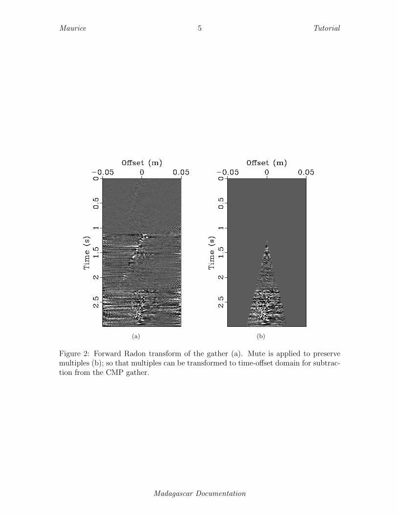
Figure 3(a) shows a CMP gather from Canterbury data set Line 12. The multipleenergy appears at time around 2.25 s. Figure 1(b) shows the same gather afterapplying NMO correction with veloctiy equals to 1500 m/s. The multiple eventsstarting at around 2.25 s and below are flatened while primary events , e.g at 2 s,are over corrected. The difference in move-out between the primaries and multiples,hence, can be used in Radon domain to attenuate multiple energy. Figure 2(a) isgenerated by forward parabolic Radon transform while Figure 1(d) is generated byinverse parabloic Radon transform. The purpose was to make sure that forward andinverse transforms do not cause any data loss.

Figure 2(a) shows the Radon transform of the CMP gather in Figure 3(a) whileFigure 2(b) shows in the Radon domain the multiple energy only after mutting theprimary energy. The protected multiples can be taken back to the time-offset domainand are subtracted from the data.


http://www.scons.org

Maurice 4 Tutorial

(a) (b)

(c) (d)

Figure 1: CMP gather from Canterbury dataset before applying NMO (a), afterapplying NMO (b), after Forward parabolic Radon transfrom (c), after applyinginverse parabolic Radon transform (d). The forward and inverse parabolic Radontransforms are applied in sequence to examine the parameters of the process and toensure that no events are lost during the process


Maurice 5 Tutorial

(a) (b)

Figure 2: Forward Radon transform of the gather (a). Mute is applied to preservemultiples (b); so that multiples can be transformed to time-offset domain for subtrac-tion from the CMP gather.


Maurice 6 Tutorial

(a) (b)

(c) (d)

Figure 3: CMP gather before multiple attenuation (a). CMP gather after multipleattenuation (b). Gather in (a) is used to generated semblance scan in (c). Gather in(b) is used to generate semblance scan in (d).


Maurice 7 Tutorial

CMP gather before multiple attenuation is shown in Figure 3(a) and the core-sponding semblance scan is shown in Figure 3(c). The CMP gather after multipleattenuation is shown in Figure 3(b) and the coresponding semblance scan is shown inFigure 3(d). The semblance scans show how multiple energy is reduced for the CMPgather after multiple attenuation.

1. To examine the forward and inverse Radon transform, Run

bash$ scons taup-qc.view

2. Edit the SConstruct file and find the line that says CHANGE ME, and modify thereference offset x0 for sfradon program. To get more details about sfradon

parameters, run

bash$ sfradon

Check your result by running

scons taup-qc.view

3. Edit the SConstruct file and find the second CHANGE ME, and modify the start-ing time t0 for sfmutter. To get more details about sfmutter parameters, runsfmutter in a Unix shell. Check your result by running

scons taup-mult.view

4. Edit the SConstruct file and find the third CHANGE ME, and modify the param-eter v0 for sfmutter. Check your result by running

scons taup-mult.view

5. Edit the SConstruct file and find the line that says ADD CODE to createsignal2.vpl. To get more details about sfgrey parameters, run sfgrey in aUnix shell. Add your code and create the vpl file by running

scons signal2.vpl

Display the figure by running

sfpen signal2.vpl

Hint: the SConstruct file has similar code for creating the figure

6. Edit the SConstruct file and find the line that says ADD CODE to displaycmp.vpl and signal2.vpl. Add your code and view the file by running


Maurice 8 Tutorial

scons cmp-signal2.view

Hint: the SConstruct file has a similar example

7. Edit the SConstruct file and find the line that says ADD CODE to displayvscan-cmp.vpl and vscan-signal2.vpl. Add your code and view the file byrunning

scons vcmp-signal2.view

Hint: the SConstruct file has a similar example

EXERCISE

In this part, your task is to apply the workflow explained above to a different CMPgather that requires different parameters. The same workflow should work here, butyou need to observe that the CMP gather used for this exercise has shallow events.This means that, after applying NMO correction, amplitudes at far offstes of theshallow events get stretched. Therefore, an additional step is required for this CMP.We need to mute the distorted amplitudes. The mute is already applied in theSConstruct.

1. Change directory to ex directory

bash$ cd ../ex

2. Display the CMP gather after NMO with and without mute applied by running

scons nmo1-nmo.view

3. Your task is to add the necessary code to attenuate multiples for this CMP. Thesame work flow used in the SConstruct file under demo directory should workhere with only changes to

• x0

• t0

• v0

where it says CHANGE ME in the comments

Hint: You will need to copy part of ../demo/Sconstruct to this SConstruct

file.


Maurice 9 Tutorial

WRITING A REPORT

1. Change directory to the parent directory

bash$ cd ..

This should be the directory that contains tutorial.tex.

2. Run

bash$ sftour scons lock

The sftour command visits all subdirectories and runs scons lock, whichcopies result files to a different location so that they do not get modified untilfurther notice.

3. You can also run

bash$ sftour scons -c

to clean intermediate results.

4. Edit the file paper.tex to include your additional results. If you have not usedLATEX before, no worries. It is a descriptive language. Study the file, and itshould become evident by example how to include figures.

5. Run

bash$ scons tutorial.pdf

and open tutorial.pdf with a PDF viewing program such as Acrobat Reader.

6. If you have LATEX2HTML installed, you can also generate an HTML version ofyour paper by running

bash$ scons tutorial.html

and opening tutorial_html/index.html in a web browser.

1 from r s f . p ro j import ∗2

3 # download cmp1 . r s f from the s e r v e r4 Fetch ( ’ cmp1 . r s f ’ , ’ cant12 ’ )5

6 # conver t to na t i v e format7 Flow ( ’cmp ’ , ’ cmp1 ’ , ’ dd form=nat ive ’ )8


Maurice 10 Tutorial

9 # crea t e cmp . vp l f i l e10 Plot ( ’cmp ’ , ’ grey t i t l e=CMP ’ )11

12 # water v e l o c i t y 1500 m/s13 wvel=150014

15 # NMO with water v e l o c i t y16 Flow ( ’nmo ’ , ’cmp ’ , ’ nmostretch h a l f=n v0=%g ’%wvel )17

18 # crea t e nmo. vp l19 Plot ( ’nmo ’ , ’ grey t i t l e=NMO’ )20

21 # crea t e cmp−nmo. vp l f i l e under Fig d i r e c t o r y22 # cmp . vp l and nmo. vp l c r ea t ed e a r l i e r us ing P lo t23 # command w i l l be p l o t e d s i d e by s i d e24 Result ( ’cmp−nmo ’ , ’cmp nmo ’ , ’ SideBySideAniso ’ )25

26 ####################27 # radon parameters28 ####################29 ox=29.2530 nx=6031 dx=2532 #−−−−−−−−−−−−−−−−−−−−−33 x0=800 # CHANGE ME34 #−−−−−−−−−−−−−−−−−−−−−35 p0=−.0536 dp=.000537 np=20138

39 # forward Radon opera tor40 radono=’ ’ ’41 radon np=%d p0=%f dp=%f x0=%d parab=y42 ’ ’ ’ %(np , p0 , dp , x0 )43

44 # inve r s e Radon opera tor45 radonoinv=’ ’ ’46 radon adj=n nx=%d ox=%g dx=%d x0=%d parab=y47 ’ ’ ’ %(nx , ox , dx , x0 )48

49 # Test radon parameters , app ly forward and50 # inve r s e Radon Transform , and QC r e s u l t s51 #########################################52 Flow ( ’ taup ’ , ’nmo ’ , radono )53


Maurice 11 Tutorial

54 # p l o t55 Plot ( ’ taup ’ , ’ grey t i t l e=forward RT’ )56

57 # Inver se58 Flow ( ’nmo2 ’ , ’ taup ’ , radonoinv )59

60 # p l o t61 Plot ( ’nmo2 ’ , ’ grey t i t l e=i n v e r s e RT’ )62

63 # Disp lay t h r e e f i g u r e s to QC Radon parameters64 # Check t ha t forward and inv e r s e Radon trans forms65 # do not change the data i . e even t s are pre served .66

67 Result ( ’ taup−qc ’ , ’nmo taup nmo2 ’ , ’ SideBySideAniso ’ )68

69 ######################################70 # des ign a mute func t i on t ha t p r o t e c t s71 # mu l t i p l e s in the Radon domain72 ######################################73 #−−−−−−−−−−−−−−−−−−−−−−−−−−−−74 t0 =1.2 # CHANGE ME ; t r y 1 .575 #−−−−−−−−−−−−−−−−−−−−−−−−−−−−76 # v e r t i c a l p o s i t i o n o f the t r i a n g l e v e r t i x77

78 #−−−−−−−−−−−−−−−−−−−−−−−−−−−−−79 v0=.03 # CHANGE ME ; t r y .01580 #−−−−−−−−−−−−−−−−−−−−−−−−−−−−−81 # s l ope o f the t r i a n g l e82

83 Flow ( ’ taupmult ’ , ’ taup ’ , ’ mutter t0=%g v0=%g ’%(t0 , v0 ) )84 Plot ( ’ taupmult ’ , ’ grey t i t l e =”mu l t i p l e s in Radon domain” ’ )85

86 # Disp lay taup . v p l and taupmult . v p l87 # This d i s p l a y a l l ow s a f l i p between88 # the two f i g u r e s89 Result ( ’ taup−mult ’ , ’ taup taupmult ’ ,90 ’ ’ ’91 cat a x i s=3 ${SOURCES[ 1 ] }92 | grey93 ’ ’ ’ )94

95 # Transform mu l i t p l e s from Radon domain to time−o f f s e t domain96 Flow ( ’ mu l t ip l e ’ , ’ taupmult ’ , radonoinv )97

98 # crea t e mu l t i p l e . v p l


Maurice 12 Tutorial

99 Plot ( ’ mu l t ip l e ’ , ’ grey t i t l e =”mu l t i p l e s ” ’ )100

101 # p l o t CMP and mu l t i p l e s s i d e by s i d e102 Result ( ’cmp−mult ’ , ’nmo2 mul t ip l e ’ , ’ SideBySideAniso ’ )103

104 # Sub t rac t mu l t i p l e s from the CMP105 Flow ( ’ s i g n a l ’ , ’ mu l t ip l e nmo2 ’ ,106 ’ ’ ’107 add s c a l e =−1,1 ${SOURCES[ 1 ] }108 ’ ’ ’ )109

110 # inve r s e NMO111 Flow ( ’ s i g n a l 2 ’ , ’ s i g n a l ’ ,112 ’ ’ ’113 nmostretch inv=y h a l f=n v0=%g114 | mutter v0=1900 x0=200115 ’ ’ ’%wvel )116

117 #−−−−−−−−−−−−−−−−−−−−−−−−−−−−−−−118 # ADD CODE to c rea t e s i g na l 2 . v p l119 #−−−−−−−−−−−−−−−−−−−−−−−−−−−−−−−120

121

122 #−−−−−−−−−−−−−−−−−−−−−−−−−−−−−−−−−−−−−−−−−−−−−123 # ADD CODE to d i s p l a y cmp . vp l and s i g na l 2 . vp l ,124 # make the f i g u r e s f l i p back and f o r t h so you125 # can examine the the r e s u l t s o f mu l t i p l e126 # at t enua t i on . Let us c a l l the output f i l e127 # cmp−s i g na l 2128 #−−−−−−−−−−−−−−−−−−−−−−−−−−−−−−−−−−−−−−−−−−−−−129

130

131 ####################132 # Semblance Scan133 ####################134 dv=10135 nv=251136 v0=1400137 vscan=’ vscan v0=%d dv=%d nv=%d semblance=y h a l f=n ’%(v0 , dv , nv )138 pick=’ p ick r e c t 1 =150 r e c t 2 =50 gate=20 ’139

140 # semblance scan141 Flow ( ’ vscan−cmp ’ , ’cmp ’ , vscan )142

143 # semblance scan


Maurice 13 Tutorial

144 Flow ( ’ vscan−s i g n a l 2 ’ , ’ s i g n a l 2 ’ , vscan )145

146 Plot ( ’ vscan−cmp ’ ,147 ’ ’ ’148 grey c o l o r=j a l l p o s=y149 t i t l e =”Ve loc i ty Scan − CMP”150 ’ ’ ’ )151

152 Plot ( ’ vscan−s i g n a l 2 ’ ,153 ’ ’ ’154 grey c o l o r=j a l l p o s=y155 t i t l e =”Ve loc i ty Scan − a f t e r demul t ip l e ”156 ’ ’ ’ )157

158 #−−−−−−−−−−−−−−−−−−−−−−−−−−−−−−−−−−−−159 # ADD CODE to d i s p l a y the two f i g u r e s160 # vscan−cmp . vp l and vscan−s i g na l 2 . v p l161 # s id e by s i d e . Let us c a l l the output162 # f i l e vcmp−s i g na l 2163 #−−−−−−−−−−−−−−−−−−−−−−−−−−−−−−−−−−−−164

165

166

167 ###################################################168 # This par t i s to c r ea t e f i g u r e s f o r t u t o r i a l . pd f169 ###################################################170 # de f i n e grey commands f o r f i g u r e s to be inc luded171 # in t u t o r i a l . pd f172 grey=’ ’ ’173 grey w a n t t i t l e=n l a b e l f a t =2 t i t l e f a t =2174 x l l =2 y l l =1.5 yur=9 xur=6175 ’ ’ ’176

177 greyc=’ ’ ’178 grey w a n t t i t l e=n l a b e l f a t =2 t i t l e f a t =2179 x l l =2 y l l =1.5 yur=9 xur=6180 c o l o r=j a l l p o s=y181 ’ ’ ’182 # crea t e p l o t s183 Result ( ’cmp ’ , grey )184 Result ( ’nmo ’ , grey )185 Result ( ’ taup ’ , grey )186 Result ( ’nmo2 ’ , grey )187 Result ( ’ taupmult ’ , grey )188 Result ( ’ s i g n a l 2 ’ , grey )


Maurice 14 Tutorial

189 Result ( ’ vscan−cmp ’ , greyc )190 Result ( ’ vscan−s i g n a l 2 ’ , greyc )191

192 End ( )

REFERENCES

Hampson, D., 1986, Inverse velocity stacking for multiple elimination: J. Can. Soc.Expl. Geophys, 22, 44–55.

Lu, H., C. S. Fulthorpe, and P. Mann, 2003, Three-dimensional architecture of shelf-building sediment drifts in the offshore canterbury basin, new zealand: MarineGeology, 193, 19 – 47.


Documents

Madagascar tutorial: Field data processing