Embed Size (px)
Citation preview

Excel©
Macros, Links and Other Good Stuff
Princeton University Excel: Macros Links and Other Good Stuff Office of Information Technology COPYRIGHT Copyright ©2001 by EZ-REF Courseware, Laguna Beach, CA http://www.ezref.com/ All rights reserved. This publication, including the student manual, instructor's guide and exercise files, or any part thereof, may not be reproduced or transmitted in any form or by any means, electronic or mechanical, without prior written permission of EZ-REF Courseware. TRADEMARKS EZ-REF is a trademark of EZ-REF Courseware. All other products or brand names mentioned are trademarks or registered trademarks of their respective holders. DISCLAIMER While EZ-REF Courseware has taken care to ensure the accuracy and quality of these materials, all material is provided without any warranty whatsoever, including, but not limited to, the implied warranties of merchantability or fitness for a particular purpose. Any persons or businesses mentioned in the text of this manual are strictly fictitious. Any resemblances to existing or deceased persons, or existing or defunct businesses, is entirely coincidental. Product Code: MS EXCEL 2002-2 01.5
Page 2 of 48
Princeton University Excel: Macros Links and Other Good Stuff Office of Information Technology
Excel Macros, Links and Other Good Stuff Table of Contents
CREATING MACROS...........................................................................................4
RECORDING THE MACRO..............................................................................4 STOPPING THE MACRO RECORDING ..........................................................7 PLAYING THE MACRO ....................................................................................8 DELETING A MACRO.....................................................................................10 ADDING MACROS TO A TOOLBAR ..............................................................12 CREATING FORM BUTTONS TO RUN AN EXCEL MACRO ........................15
LINKING FILES...................................................................................................17
EDITING LINKS ..............................................................................................19
WORKING WITH MULTIPLE SHEETS ..............................................................22
MOVING BETWEEN WORKSHEETS.............................................................22 NAMING WORKSHEETS ...............................................................................23 MOVING A WORKSHEET ..............................................................................24 COPYING A WORKSHEET ............................................................................24 DELETING A WORKSHEET...........................................................................25 INSERTING A NEW WORKSHEET ................................................................26 GROUPING SHEETS .....................................................................................27 CREATING 3-D FORMULAS ..........................................................................28 MOVING/COPYING FROM ONE WORKSHEET TO ANOTHER....................29 HIDING/UNHIDING GROUPS.........................................................................29
CONSOLIDATING DATA....................................................................................31
USING THE GOAL SEEK...................................................................................35
THE SCENARIO MANAGER..............................................................................37
CREATING A SCENARIO...............................................................................37 DISPLAYING A SCENARIO............................................................................41 EDITING A SCENARIO...................................................................................42 MERGING SCENARIOS .................................................................................44 CREATING SCENARIO SUMMARY REPORTS.............................................46 DELETING A SCENARIO ...............................................................................48
Page 3 of 48
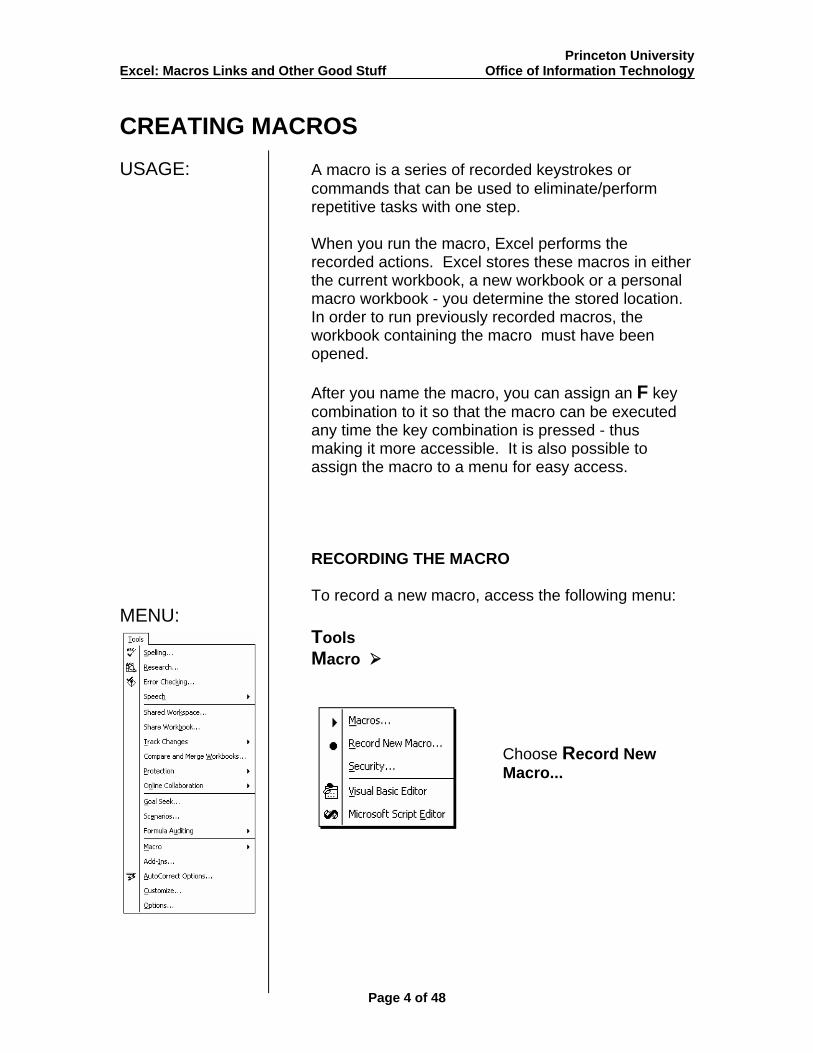
Princeton University Excel: Macros Links and Other Good Stuff Office of Information Technology CREATING MACROS USAGE: A macro is a series of recorded keystrokes or
commands that can be used to eliminate/perform repetitive tasks with one step.
When you run the macro, Excel performs the recorded actions. Excel stores these macros in either the current workbook, a new workbook or a personal macro workbook - you determine the stored location. In order to run previously recorded macros, the workbook containing the macro must have been opened.
After you name the macro, you can assign an F key combination to it so that the macro can be executed any time the key combination is pressed - thus making it more accessible. It is also possible to assign the macro to a menu for easy access.
RECORDING THE MACRO
To record a new macro, access the following menu:
MENU: Tools T
Macro
Choose Record New Macro...
Page 4 of 48
Princeton University Excel: Macros Links and Other Good Stuff Office of Information Technology
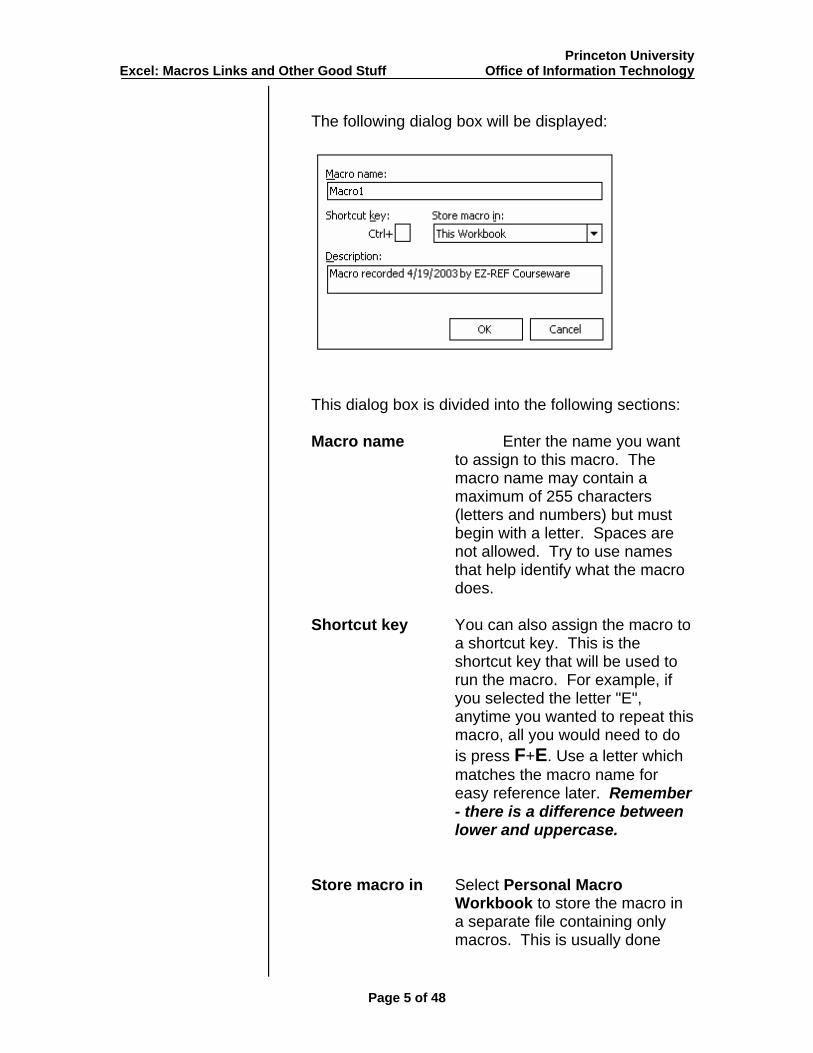
The following dialog box will be displayed:
This dialog box is divided into the following sections:
Macro name Enter the name you want to assign to this macro. The macro name may contain a maximum of 255 characters (letters and numbers) but must begin with a letter. Spaces are not allowed. Try to use names that help identify what the macro does.
Shortcut key You can also assign the macro to
a shortcut key. This is the shortcut key that will be used to run the macro. For example, if you selected the letter "E", anytime you wanted to repeat this macro, all you would need to do is press F+E. Use a letter which matches the macro name for easy reference later. Remember - there is a difference between lower and uppercase.
Store macro in Select Personal Macro Workbook to store the macro in a separate file containing only macros. This is usually done
Page 5 of 48
Princeton University Excel: Macros Links and Other Good Stuff Office of Information Technology
when creating generic macros that you will want to access from any workbook.
Select This Workbook if you want to create a macro associated solely with the current file.
It is also possible to create a New Workbook if the current one is full.
Description Use this section to further define specific information about the macro being recorded.
Once you have entered the information, select
.
Once you close the dialog box, you are returned to the worksheet. The word Recording appears in the bottom left corner of the status line reminding you that you are in the midst of recording.
Enter the keystrokes/menu options that will make up the macro.
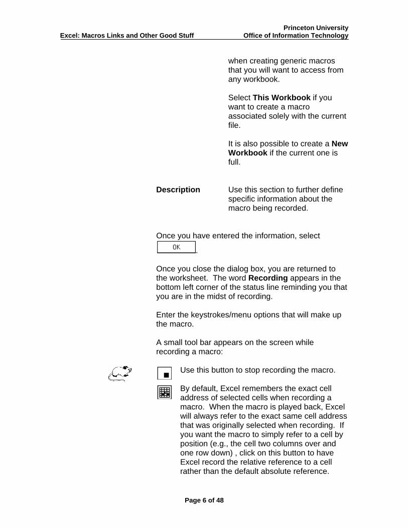
A small tool bar appears on the screen while recording a macro:
Use this button to stop recording the macro.
By default, Excel remembers the exact cell address of selected cells when recording a macro. When the macro is played back, Excel will always refer to the exact same cell address that was originally selected when recording. If you want the macro to simply refer to a cell by position (e.g., the cell two columns over and one row down) , click on this button to have Excel record the relative reference to a cell rather than the default absolute reference.
Page 6 of 48
Princeton University Excel: Macros Links and Other Good Stuff Office of Information Technology
NOTE: Keep in mind while creating your macro that Excel will record everything, including your mistakes!!
STOPPING THE MACRO RECORDING
Once the macro is complete, you will need to stop the recording.
The easiest way to stop the macro is to click on this button which appears in a small window in the right corner of your screen when recording a macro.
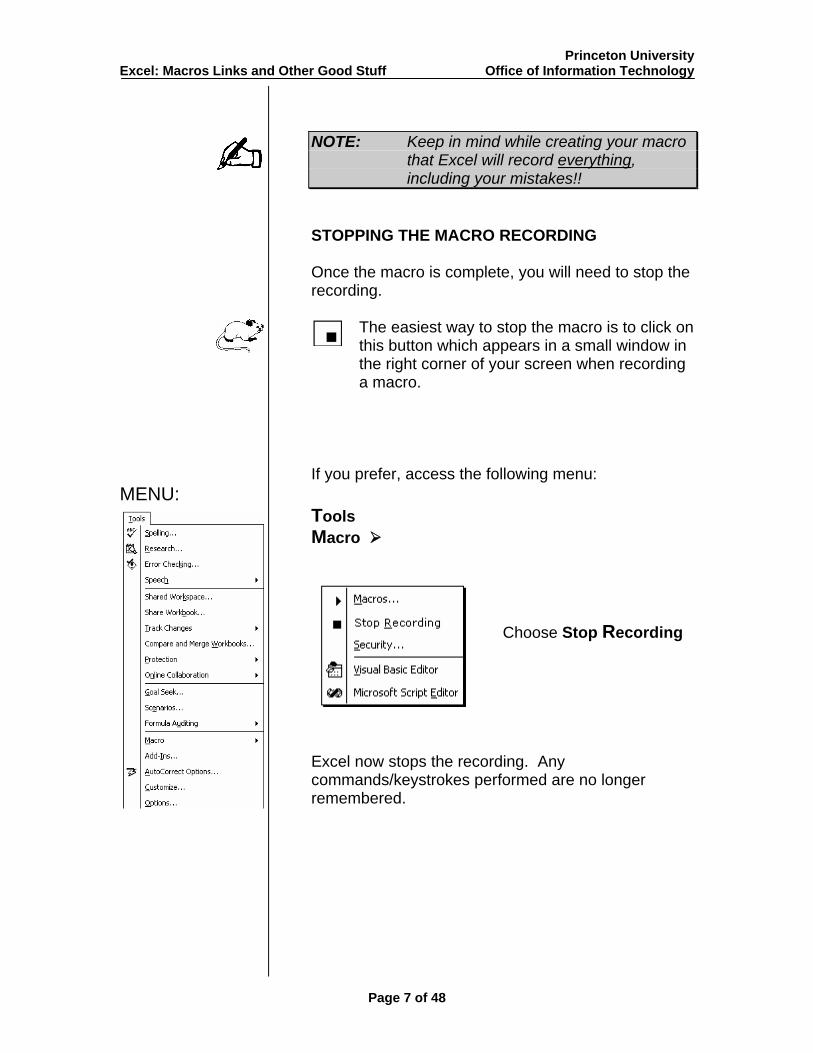
If you prefer, access the following menu: MENU:
Tools T
Macro
Choose Stop Recording
Excel now stops the recording. Any commands/keystrokes performed are no longer remembered.
Page 7 of 48
Princeton University Excel: Macros Links and Other Good Stuff Office of Information Technology
NOTE: Be sure to look at the status bar to ensure that the word Recording has been removed.
PLAYING THE MACRO
Once the macro has been recorded, you can play it anytime you need the steps contained in the macro repeated. If you stored the macro in an outside workbook, you will need to be sure that the workbook is open before continuing.
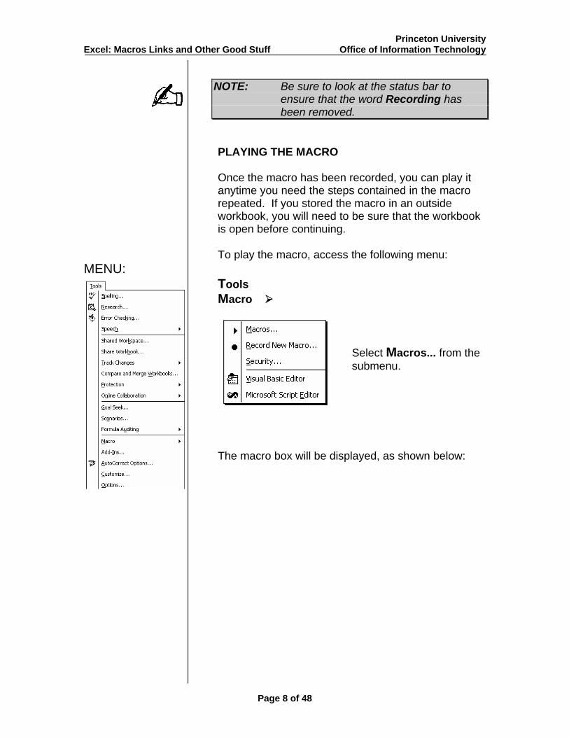
To play the macro, access the following menu:
MENU: Tools T
Macro
Select Macros... from the submenu.
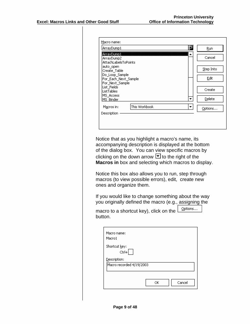
The macro box will be displayed, as shown below:
Page 8 of 48
Princeton University Excel: Macros Links and Other Good Stuff Office of Information Technology
Notice that as you highlight a macro’s name, its accompanying description is displayed at the bottom of the dialog box. You can view specific macros by clicking on the down arrow to the right of the Macros in box and selecting which macros to display.
Notice this box also allows you to run, step through macros (to view possible errors), edit, create new ones and organize them.
If you would like to change something about the way you originally defined the macro (e.g., assigning the
macro to a shortcut key), click on the button.
Page 9 of 48
Princeton University Excel: Macros Links and Other Good Stuff Office of Information Technology
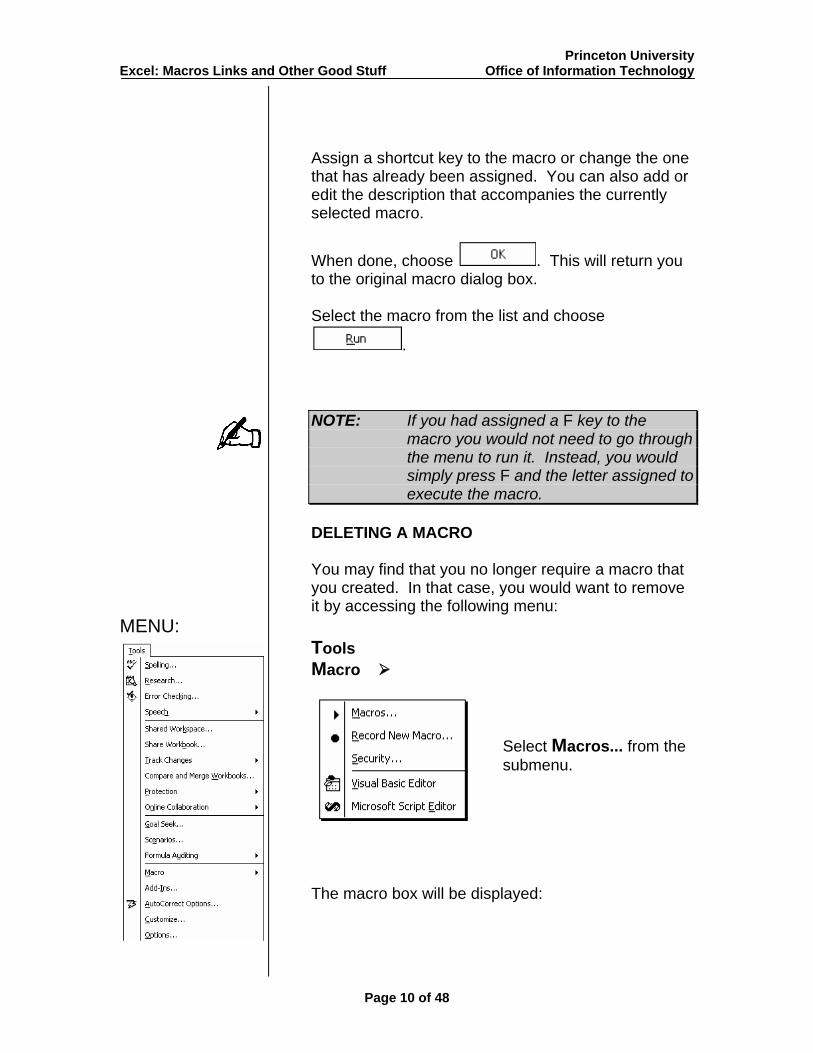
Assign a shortcut key to the macro or change the one that has already been assigned. You can also add or edit the description that accompanies the currently selected macro.
When done, choose . This will return you to the original macro dialog box.
Select the macro from the list and choose
.
NOTE: If you had assigned a F key to the macro you would not need to go through the menu to run it. Instead, you would simply press F and the letter assigned to execute the macro.
DELETING A MACRO
You may find that you no longer require a macro that you created. In that case, you would want to remove it by accessing the following menu:
MENU: Tools T
Macro
Select Macros... from the submenu.
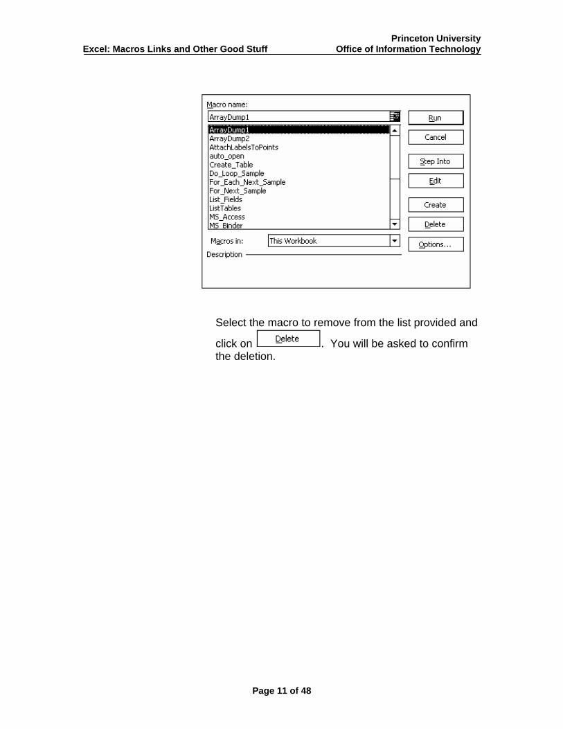
The macro box will be displayed:
Page 10 of 48
Princeton University Excel: Macros Links and Other Good Stuff Office of Information Technology
Select the macro to remove from the list provided and
click on . You will be asked to confirm the deletion.
Page 11 of 48
Princeton University Excel: Macros Links and Other Good Stuff Office of Information Technology
ADDING MACROS TO A TOOLBAR
You may wish to run your macors by adding them to one of Excel’s toolbars, or by creating a custom toolbar just for your macros. To customize the toolbar, follow the steps outlined below:
Point to a blank spot on any tool bar displayed
on your screen and then click the [RIGHT] mouse button once.
Select Customize... from the pop-up menu
that appears.
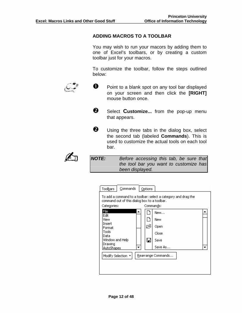
Using the three tabs in the dialog box, select the second tab (labeled Commands). This is used to customize the actual tools on each tool bar.
NOTE: Before accessing this tab, be sure that
the tool bar you want to customize has been displayed.
Page 12 of 48
Princeton University Excel: Macros Links and Other Good Stuff Office of Information Technology
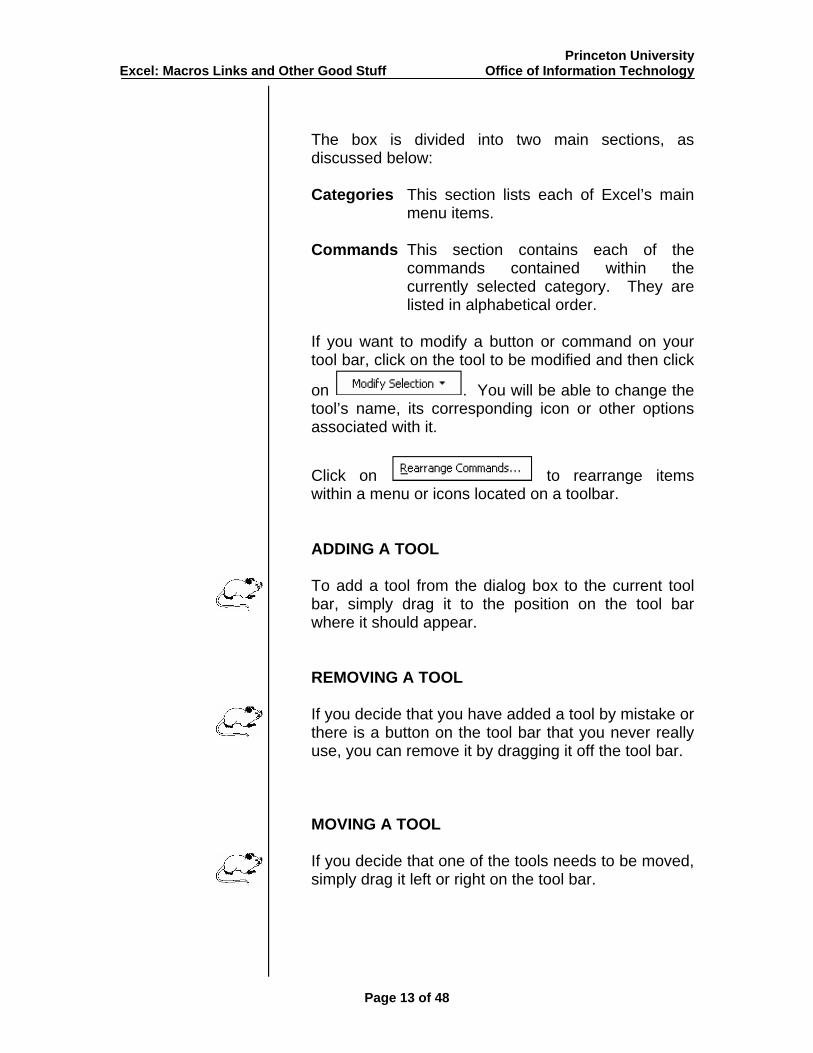
The box is divided into two main sections, as discussed below:
Categories This section lists each of Excel’s main
menu items.
Commands This section contains each of the commands contained within the currently selected category. They are listed in alphabetical order.
If you want to modify a button or command on your tool bar, click on the tool to be modified and then click
on . You will be able to change the tool’s name, its corresponding icon or other options associated with it.
Click on to rearrange items within a menu or icons located on a toolbar. ADDING A TOOL
To add a tool from the dialog box to the current tool bar, simply drag it to the position on the tool bar where it should appear.
REMOVING A TOOL
If you decide that you have added a tool by mistake or there is a button on the tool bar that you never really use, you can remove it by dragging it off the tool bar.
MOVING A TOOL
If you decide that one of the tools needs to be moved, simply drag it left or right on the tool bar.
Page 13 of 48

Princeton University Excel: Macros Links and Other Good Stuff Office of Information Technology
When done, click on to save the tool bar changes, close the dialog box and return to your workbook.
Page 14 of 48
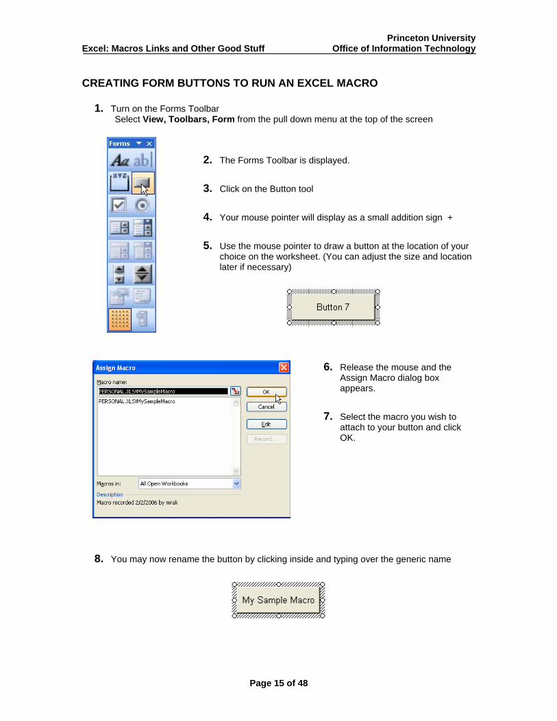
Princeton University Excel: Macros Links and Other Good Stuff Office of Information Technology CREATING FORM BUTTONS TO RUN AN EXCEL MACRO
1. Turn on the Forms Toolbar Select View, Toolbars, Form from the pull down menu at the top of the screen
2. The Forms Toolbar is displayed.
3. Click on the Button tool
4. Your mouse pointer will display as a small addition sign +
5. Use the mouse pointer to draw a button at the location of your choice on the worksheet. (You can adjust the size and location later if necessary)
6. Release the mouse and the Assign Macro dialog box appears.
7. Select the macro you wish to attach to your button and click OK.
8. You may now rename the button by clicking inside and typing over the generic name
Page 15 of 48

Princeton University Excel: Macros Links and Other Good Stuff Office of Information Technology
9. To size or relocate the macro, you must first be sure that it is selected, but not in typing mode. This means that if you have just completed changing its name, you will need to click anywhere on the border of the button to change to select mode. Note that the border of the button appears differently in typing mode than it does in select mode.
Button in typing mode
Button in select mode
10. Once the button in is select mode, you may drag it to relocate it or drag one of the "handles" to resize it.
Click and drag on the border to move the button.
Click and drag on a handle to resize the button.
11. If you wish to format the button (change font color, size, etc), click your right mouse button on the button and choose Format Control from the pop-up menu.
Page 16 of 48
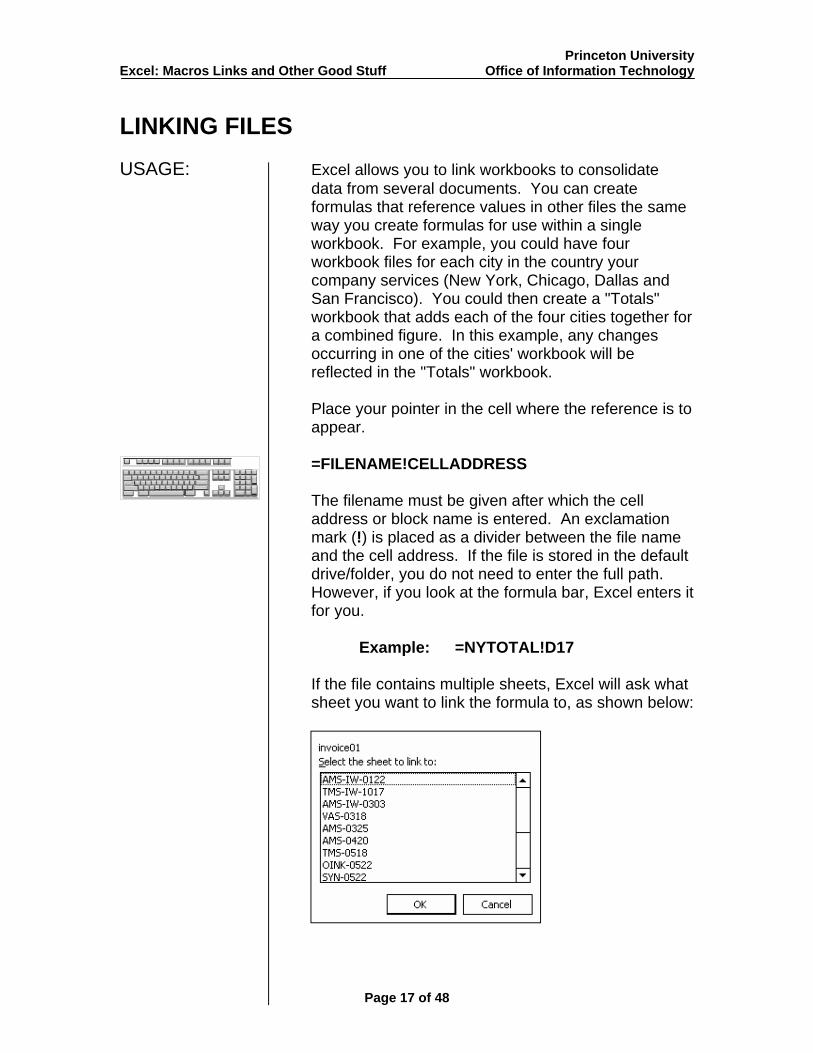
Princeton University Excel: Macros Links and Other Good Stuff Office of Information Technology LINKING FILES USAGE: Excel allows you to link workbooks to consolidate
data from several documents. You can create formulas that reference values in other files the same way you create formulas for use within a single workbook. For example, you could have four workbook files for each city in the country your company services (New York, Chicago, Dallas and San Francisco). You could then create a "Totals" workbook that adds each of the four cities together for a combined figure. In this example, any changes occurring in one of the cities' workbook will be reflected in the "Totals" workbook.
Place your pointer in the cell where the reference is to appear.
=FILENAME!CELLADDRESS
The filename must be given after which the cell address or block name is entered. An exclamation mark (!) is placed as a divider between the file name and the cell address. If the file is stored in the default drive/folder, you do not need to enter the full path. However, if you look at the formula bar, Excel enters it for you.
Example: =NYTOTAL!D17
If the file contains multiple sheets, Excel will ask what sheet you want to link the formula to, as shown below:
Page 17 of 48
Princeton University Excel: Macros Links and Other Good Stuff Office of Information Technology
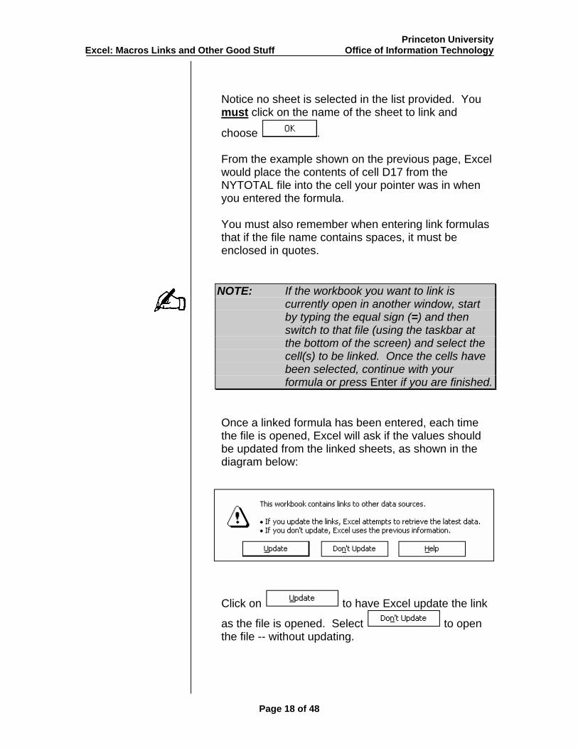
Notice no sheet is selected in the list provided. You must click on the name of the sheet to link and
choose . From the example shown on the previous page, Excel would place the contents of cell D17 from the NYTOTAL file into the cell your pointer was in when you entered the formula.
You must also remember when entering link formulas that if the file name contains spaces, it must be enclosed in quotes.
NOTE: If the workbook you want to link is currently open in another window, start by typing the equal sign (=) and then switch to that file (using the taskbar at the bottom of the screen) and select the cell(s) to be linked. Once the cells have been selected, continue with your formula or press Enter if you are finished.
Once a linked formula has been entered, each time the file is opened, Excel will ask if the values should be updated from the linked sheets, as shown in the diagram below:
Click on to have Excel update the link
as the file is opened. Select to open the file -- without updating.
Page 18 of 48
Princeton University Excel: Macros Links and Other Good Stuff Office of Information Technology
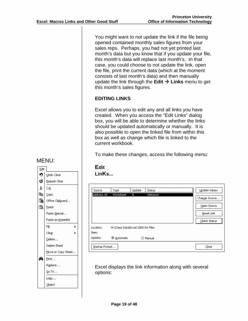
You might want to not update the link if the file being opened contained monthly sales figures from your sales reps. Perhaps, you had not yet printed last month’s data but you know that if you update your file, this month’s data will replace last month’s. In that case, you could choose to not update the link, open the file, print the current data (which at the moment consists of last month’s data) and then manually update the link through the Edit Links menu to get this month’s sales figures. EDITING LINKS
Excel allows you to edit any and all links you have created. When you access the “Edit Links” dialog box, you will be able to determine whether the links should be updated automatically or manually. It is also possible to open the linked file from within this box as well as change which file is linked to the current workbook.
To make these changes, access the following menu:
MENU: Edit LinKs...
Excel displays the link information along with several options:
Page 19 of 48
Princeton University Excel: Macros Links and Other Good Stuff Office of Information Technology
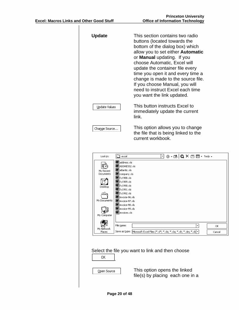
Update This section contains two radio buttons (located towards the bottom of the dialog box) which allow you to set either Automatic or Manual updating. If you choose Automatic, Excel will update the container file every time you open it and every time a change is made to the source file. If you choose Manual, you will need to instruct Excel each time you want the link updated.
This button instructs Excel to immediately update the current link. This option allows you to change the file that is being linked to the current workbook.
Select the file you want to link and then choose
.
This option opens the linked file(s) by placing each one in a
Page 20 of 48
Princeton University Excel: Macros Links and Other Good Stuff Office of Information Technology
different window. You may, then, edit the file(s) as needed.
Click on this button to break the link between the files and insert the last known value in the previously linked cell.
Click on this button to verify the link to ensure it is still valid.
Once all settings have been made within the Edit Links dialog box, choose to return to your workbook.
Page 21 of 48
Princeton University Excel: Macros Links and Other Good Stuff Office of Information Technology WORKING WITH MULTIPLE SHEETS USAGE: You can organize your work by keeping related
information on separate worksheets within the same file (workbook). You might, for example, create a file with 4 worksheets, one for each quarter.
You can insert worksheets just as you can insert additional rows and columns. Each file can have up to 256 "sheets". Each new file automatically contains three worksheets.
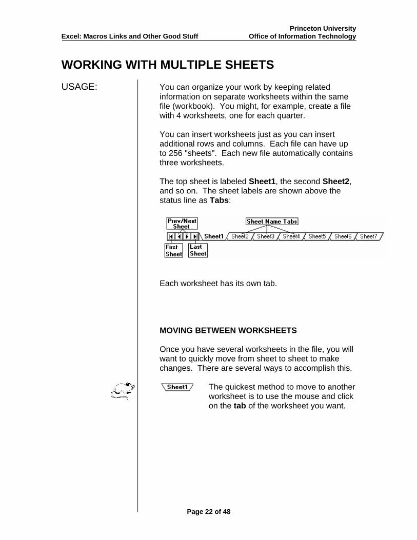
The top sheet is labeled Sheet1, the second Sheet2, and so on. The sheet labels are shown above the status line as Tabs:
Each worksheet has its own tab.
MOVING BETWEEN WORKSHEETS
Once you have several worksheets in the file, you will want to quickly move from sheet to sheet to make changes. There are several ways to accomplish this.
The quickest method to move to another worksheet is to use the mouse and click on the tab of the worksheet you want.
Page 22 of 48
Princeton University Excel: Macros Links and Other Good Stuff Office of Information Technology
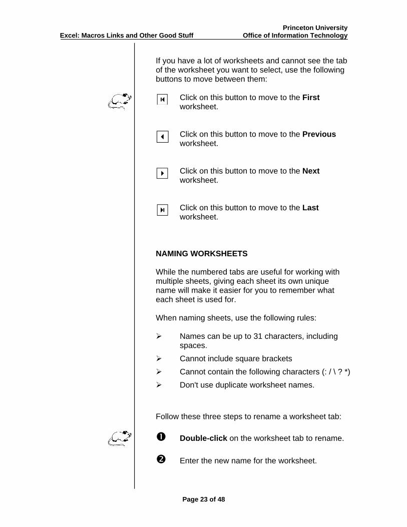
If you have a lot of worksheets and cannot see the tab of the worksheet you want to select, use the following buttons to move between them:
Click on this button to move to the First worksheet.
Click on this button to move to the Previous worksheet.
Click on this button to move to the Next worksheet.
Click on this button to move to the Last worksheet.
NAMING WORKSHEETS
While the numbered tabs are useful for working with multiple sheets, giving each sheet its own unique name will make it easier for you to remember what each sheet is used for.
When naming sheets, use the following rules:
Names can be up to 31 characters, including
spaces. Cannot include square brackets Cannot contain the following characters (: / \ ? *) Don't use duplicate worksheet names.
Follow these three steps to rename a worksheet tab:
Double-click on the worksheet tab to rename.
Enter the new name for the worksheet.
Page 23 of 48
Princeton University Excel: Macros Links and Other Good Stuff Office of Information Technology
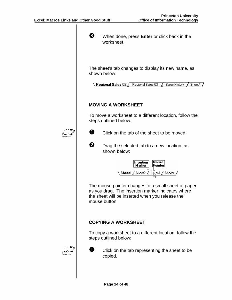
When done, press Enter or click back in the worksheet.
The sheet's tab changes to display its new name, as shown below:
MOVING A WORKSHEET
To move a worksheet to a different location, follow the steps outlined below:
Click on the tab of the sheet to be moved.
Drag the selected tab to a new location, as
shown below:
The mouse pointer changes to a small sheet of paper as you drag. The insertion marker indicates where the sheet will be inserted when you release the mouse button.
COPYING A WORKSHEET
To copy a worksheet to a different location, follow the steps outlined below:
Click on the tab representing the sheet to be
copied.
Page 24 of 48
Princeton University Excel: Macros Links and Other Good Stuff Office of Information Technology
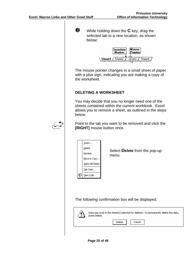
While holding down the C key, drag the selected tab to a new location, as shown below:
The mouse pointer changes to a small sheet of paper with a plus sign, indicating you are making a copy of the worksheet. DELETING A WORKSHEET
You may decide that you no longer need one of the sheets contained within the current workbook. Excel allows you to remove a sheet, as outlined in the steps below:
Point to the tab you want to be removed and click the [RIGHT] mouse button once.
Select Delete from the pop-up menu.
The following confirmation box will be displayed:
Page 25 of 48

Princeton University Excel: Macros Links and Other Good Stuff Office of Information Technology
You will be asked to confirm the deletion.
NOTE: Be sure you want to permanently delete the worksheet as you will not be able to undo this action!
INSERTING A NEW WORKSHEET
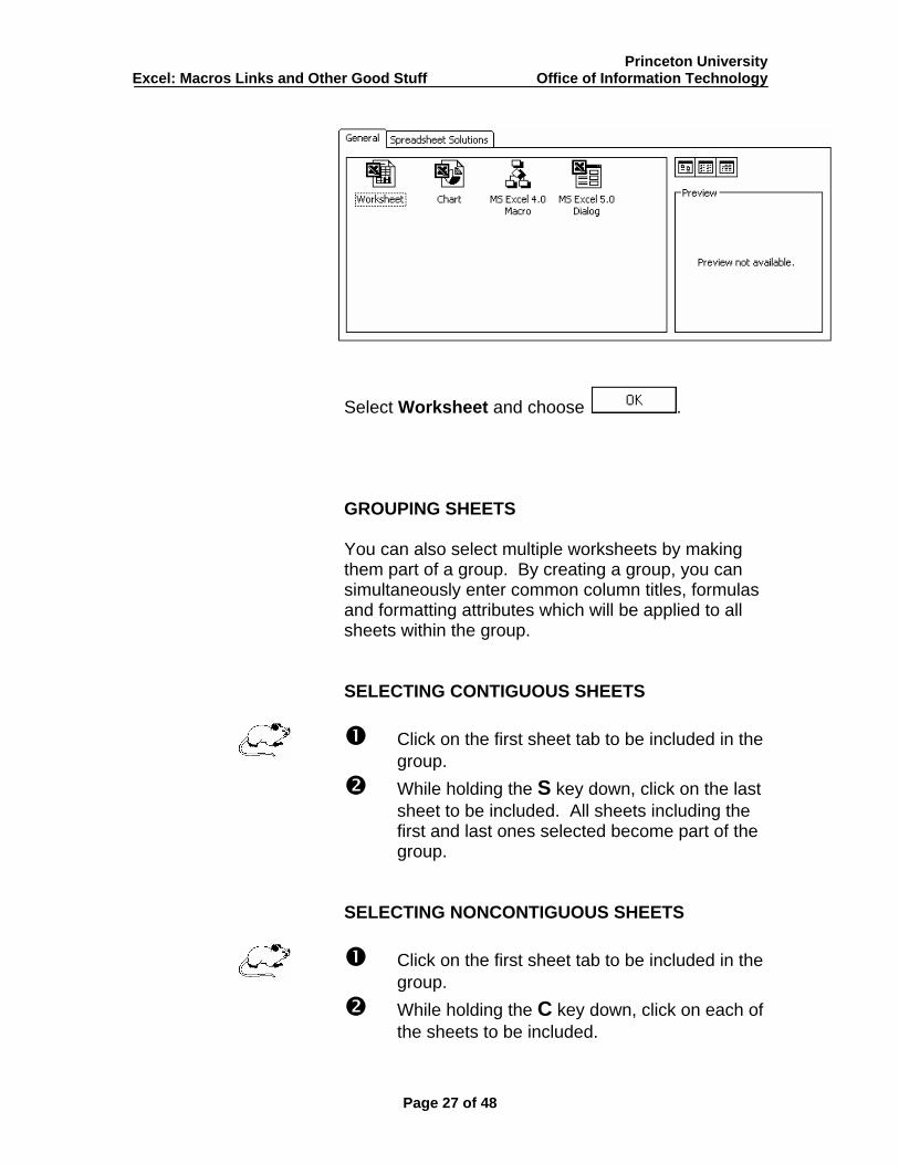
By default, each workbook automatically contains three tabs. To add a new sheet, follow these steps:
Point to the tab which you would like to insert the sheet in front of and click the [RIGHT] mouse button.
Select Insert... from the pop-up menu.
The following dialog box will be displayed:
Page 26 of 48
Princeton University Excel: Macros Links and Other Good Stuff Office of Information Technology
Select Worksheet and choose . GROUPING SHEETS
You can also select multiple worksheets by making them part of a group. By creating a group, you can simultaneously enter common column titles, formulas and formatting attributes which will be applied to all sheets within the group.
SELECTING CONTIGUOUS SHEETS
Click on the first sheet tab to be included in the group.
While holding the S key down, click on the last sheet to be included. All sheets including the first and last ones selected become part of the group.
SELECTING NONCONTIGUOUS SHEETS
Click on the first sheet tab to be included in the group.
While holding the C key down, click on each of the sheets to be included.
Page 27 of 48
Princeton University Excel: Macros Links and Other Good Stuff Office of Information Technology
NOTE: When you group sheets, Excel displays the word [Group] to the right of the file name within the title bar.
WORKING WITH GROUPED SHEETS
Once you have a set of worksheets grouped, any formatting you apply to the top sheet will automatically be applied to all other sheets. You can also apply formulas and labels to the same cell address within each sheet of the group. Simply enter the formula/text label on the first sheet and Excel will automatically copy it to the same cell in all other sheets.
CREATING 3-D FORMULAS
Creating a three-dimensional formula is similar to linking a cell to another cell in an external workbook. The difference is that you will be linking to one or more sheets within the same workbook. To link a formula to a cell in another sheet, simply begin the formula as you normally would and when the external cell is required, click on the tab of the sheet to be included in the formula and then select the required cell.
To create formula that references the same cell (e.g., B10) within multiple sheets, click on the tab representing the first sheet to be included in the formula and hold the S key down as you click on the tab of the last sheet to be included. Next, select the cell(s) you want to include from each of the selected sheets within the formula.
NOTE: This only works when selecting
contiguous sheets!
For example, including cell B10 of sheets 2-6 in a sum formula would look like the example shown below:
Page 28 of 48
Princeton University Excel: Macros Links and Other Good Stuff Office of Information Technology
=SUM('Sheet2:Sheet6'!B10)
Notice the colon separating the first and last sheet in the group.
MOVING/COPYING FROM ONE WORKSHEET TO ANOTHER
You can also move a block of cells by selecting the block and then (while holding down the Alt key), dragging the block to another worksheet. If you also hold down the Ctrl key, the block will be copied (instead of moved) onto another worksheet. HIDING/UNHIDING GROUPS
If a worksheet contains only formulas or data that are used by other sheets within the workbook, you may want to hide that worksheet to prevent accidental changes from being made. You can also hide sheets that contain sensitive material (e.g., salaries, commissions). Hidden sheets can still be used in formulas.
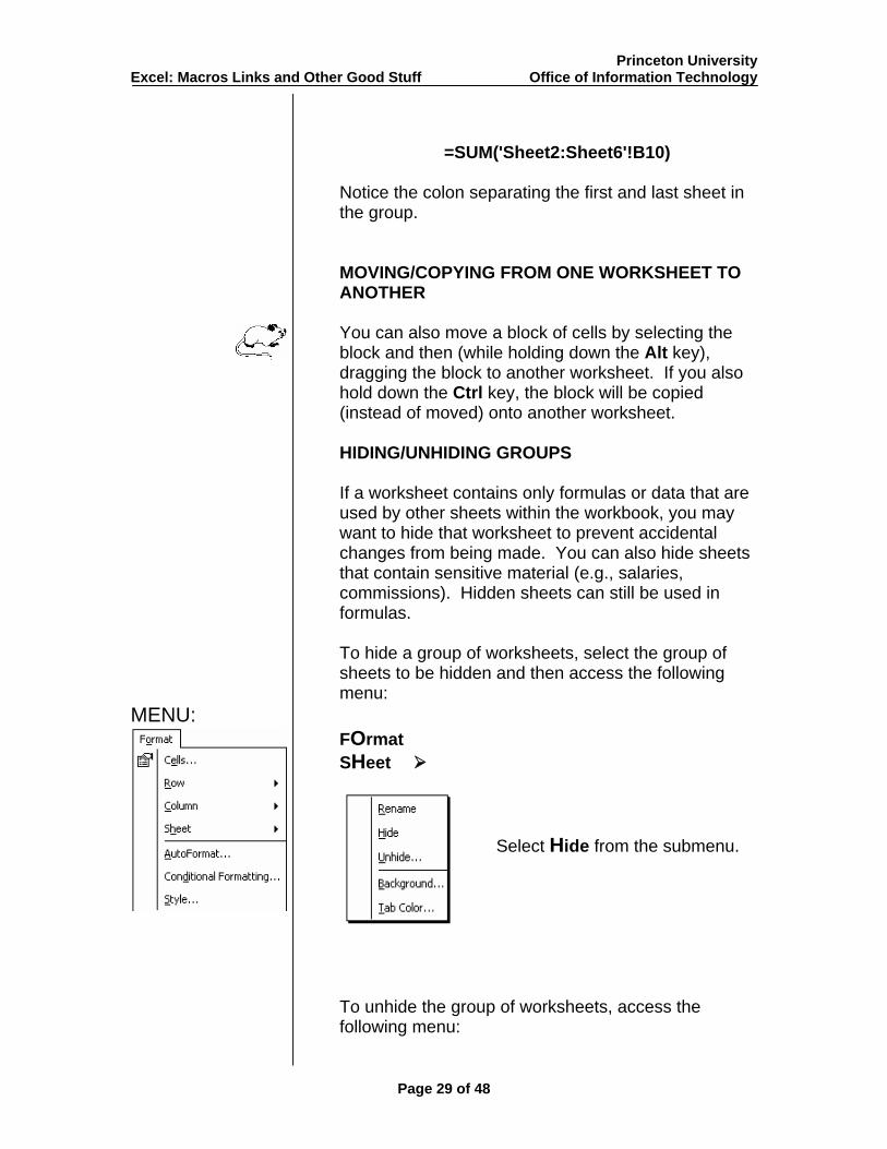
To hide a group of worksheets, select the group of sheets to be hidden and then access the following menu:
MENU: FOrmat SHeet
Select Hide from the submenu.
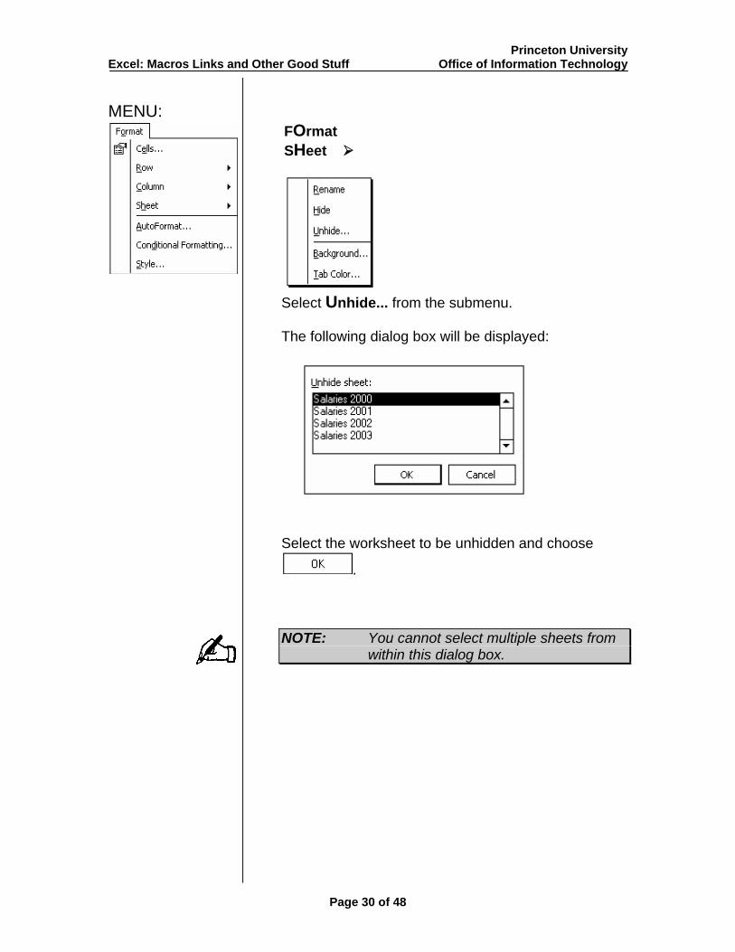
To unhide the group of worksheets, access the following menu:
Page 29 of 48
Princeton University Excel: Macros Links and Other Good Stuff Office of Information Technology MENU:
FOrmat SHeet
Select Unhide... from the submenu. The following dialog box will be displayed:
Select the worksheet to be unhidden and choose
.
NOTE: You cannot select multiple sheets from within this dialog box.
Page 30 of 48
Princeton University Excel: Macros Links and Other Good Stuff Office of Information Technology CONSOLIDATING DATA USAGE: The Consolidate command is used to do exactly
what its name implies - to consolidate information from many sources (up to 255) into one. For example, if you were interested in obtaining statistical data from various offices across the country so that you could create a workbook based solely on their totals, you could use the consolidate command to combine the individual office totals into one grand total.
You may also add a link between the consolidated workbook and its supporting files so that any time a change is made to one of the supporting worksheets, the consolidated file is automatically updated to reflect that change.
When you instruct Excel to consolidate, you will be asked whether to consolidate by position or by category.
If you choose to consolidate by position, Excel combines the data from the same cell address in each of the supporting worksheets. This means that the data you want consolidated must be in the same cell in each workbook.
However, if you choose to consolidate by category, you can have the data in different cell addresses. Excel simply consolidates the information based on common category headings, no matter what column or row they are located in.
NOTE: When consolidating by category, Excel does not care what column the source data is stored in. However, the category labels must be located either in the first row or in the leftmost column of the source range.
Before continuing, be sure you are in the workbook you want to contain the consolidated information.
Page 31 of 48
Princeton University Excel: Macros Links and Other Good Stuff Office of Information Technology
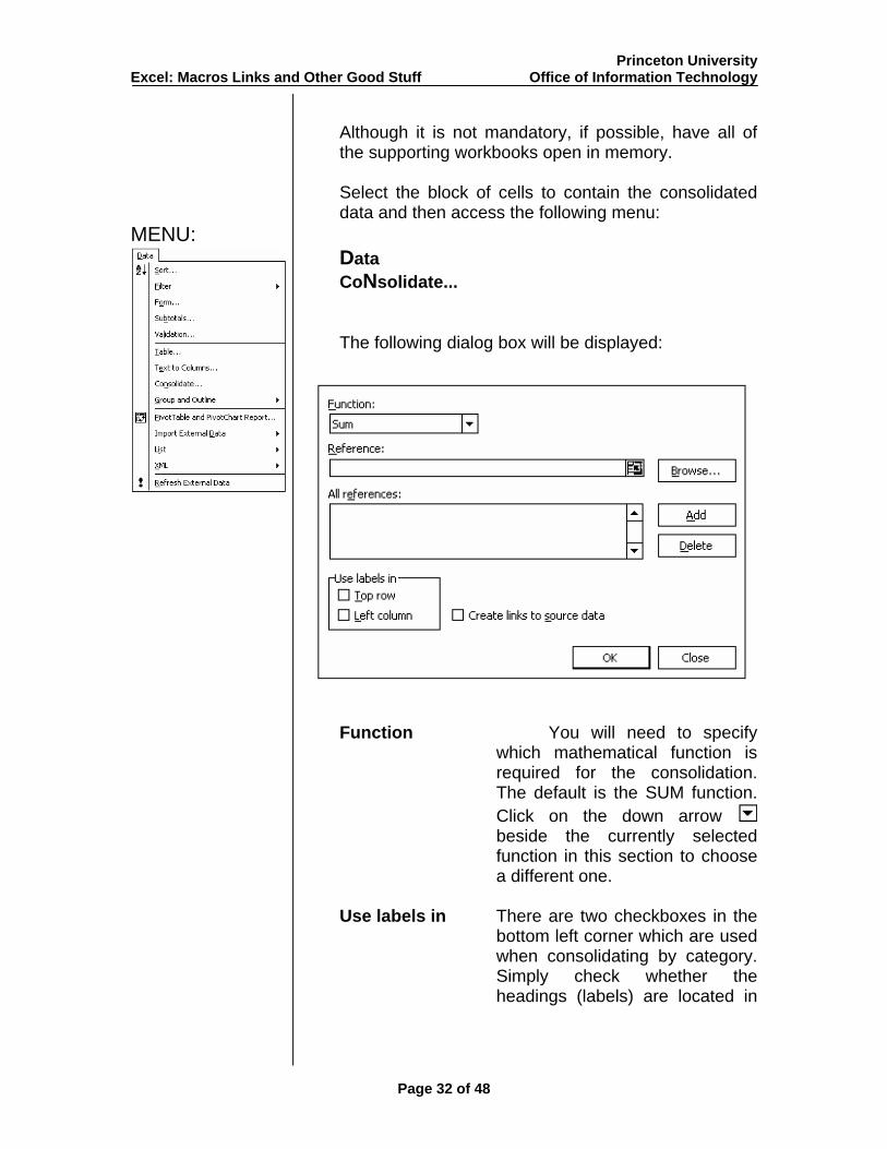
Although it is not mandatory, if possible, have all of the supporting workbooks open in memory. Select the block of cells to contain the consolidated data and then access the following menu:
MENU: Data CoNsolidate...
The following dialog box will be displayed:
Function You will need to specify which mathematical function is required for the consolidation. The default is the SUM function. Click on the down arrow beside the currently selected function in this section to choose a different one.
Use labels in There are two checkboxes in the
bottom left corner which are used when consolidating by category. Simply check whether the headings (labels) are located in
Page 32 of 48
Princeton University Excel: Macros Links and Other Good Stuff Office of Information Technology
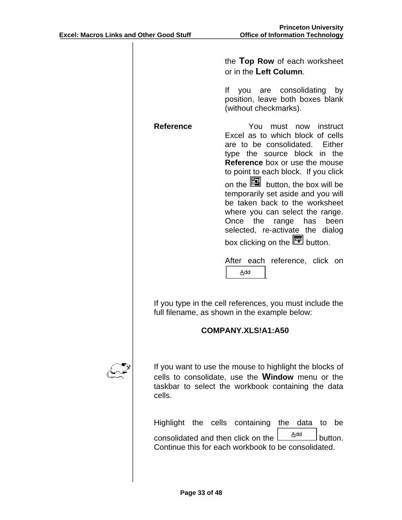
the Top Row of each worksheet or in the
T
Left Column.
If you are consolidating by position, leave both boxes blank (without checkmarks).
Reference You must now instruct
Excel as to which block of cells are to be consolidated. Either type the source block in the Reference box or use the mouse to point to each block. If you click on the button, the box will be temporarily set aside and you will be taken back to the worksheet where you can select the range. Once the range has been selected, re-activate the dialog box clicking on the button.
After each reference, click on
.
If you type in the cell references, you must include the full filename, as shown in the example below:
COMPANY.XLS!A1:A50
If you want to use the mouse to highlight the blocks of cells to consolidate, use the Window menu or the taskbar to select the workbook containing the data cells.
Highlight the cells containing the data to be
consolidated and then click on the button. Continue this for each workbook to be consolidated.
Page 33 of 48
Princeton University Excel: Macros Links and Other Good Stuff Office of Information Technology
At the bottom of the dialog box you will see a checkbox which is used to Create links to Source data. If you choose this option, Excel will create a link to each cell being consolidated so that changes in the worksheets will automatically be updated in the main worksheet.
After making the necessary selections, choose
.
Page 34 of 48

Princeton University Excel: Macros Links and Other Good Stuff Office of Information Technology USING THE GOAL SEEK USAGE: The Goal Seek is used within Excel to create
worksheets that have a final goal in mind but do not have the input to solve the problem. For example, if you were considering purchasing a new car and knew the maximum monthly payment amount you could make, it would be possible to use “Goal Seek” to determine what size loan you could afford. Basically, you are working backwards from an answer to determine the input values needed to achieve that answer.
Select the cell containing the final answer (i.e., the maximum monthly loan payment) and then access the following menu:
MENU: Tools T
Goal Seek...
The following dialog box will be displayed:
The Set cell section should include the address of the cell containing the formula for which you want to find a solution. Click on to return to the worksheet to select the cell.
To value refers to the new value you are trying to reach (i.e., the monthly payment amount you could afford).
By changing cell refers to the address containing the value you want Excel to change to achieve the
Page 35 of 48
Princeton University Excel: Macros Links and Other Good Stuff Office of Information Technology
desired answer (i.e., the loan amount). Click on to return to the worksheet to select the cell.
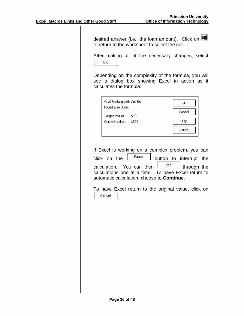
After making all of the necessary changes, select
. Depending on the complexity of the formula, you will see a dialog box showing Excel in action as it calculates the formula:
If Excel is working on a complex problem, you can
click on the button to interrupt the
calculation. You can then through the calculations one at a time. To have Excel return to automatic calculation, choose to Continue.
To have Excel return to the original value, click on
.
Page 36 of 48
Princeton University Excel: Macros Links and Other Good Stuff Office of Information Technology THE SCENARIO MANAGER USAGE: Scenarios are sets of different data for the same block
of cells. They are used to perform what-if calculations. For example, a worst-case scenario shows what value would result if the least desirable set of variables were placed in the model. On the other hand, a best-case scenario displays the value that would result if the most desirable set of variables were placed in the model. A most-likely scenario displays the value that would result if the most likely set of variables were placed in the model.
A scenario is simply a way of storing multiple sets of numbers that can quickly be recalled and displayed. This allows you to play “what if we looked at this scenario” type of games. You can easily select from a group of previously saved scenarios.
Each sheet in a workbook can have its own set of scenarios. For example, if you have a workbook with six worksheets (all with different products and sales statistics), you might want to construct a different scenario for each sheet. In each scenario, you can create models for best-case, worst-case and most-likely sales of each product.
Excel also can be used to create a pivot table report of your scenarios. The pivot table report lets you mix and match scenarios and then view the effects of these scenarios. This allows you to view a scenario with a different perspective.
CREATING A SCENARIO
To create a scenario, follow the steps outlined below:
Create your spreadsheet with the first set of values that should be recorded as a scenario.
Page 37 of 48
Princeton University Excel: Macros Links and Other Good Stuff Office of Information Technology
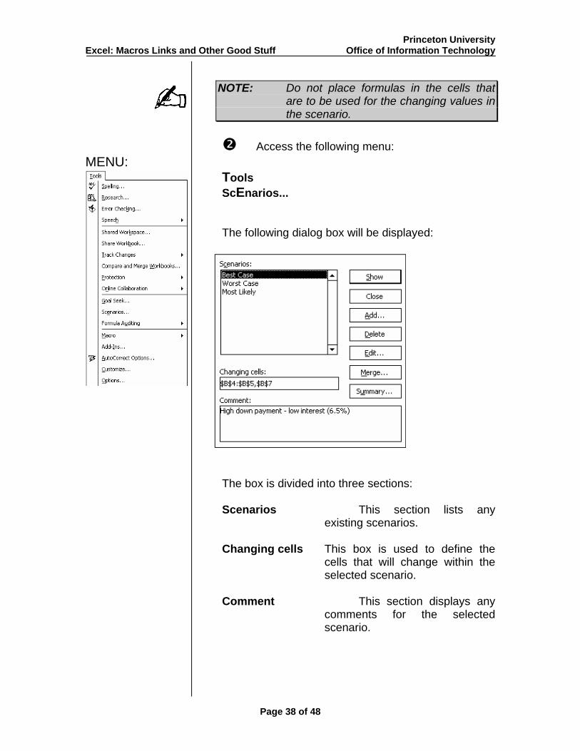
NOTE: Do not place formulas in the cells that are to be used for the changing values in the scenario.
Access the following menu:
MENU: Tools T
ScEnarios...
The following dialog box will be displayed:
The box is divided into three sections:
Scenarios This section lists any
existing scenarios.
Changing cells This box is used to define the cells that will change within the selected scenario.
Comment This section displays any
comments for the selected scenario.
Page 38 of 48
Princeton University Excel: Macros Links and Other Good Stuff Office of Information Technology
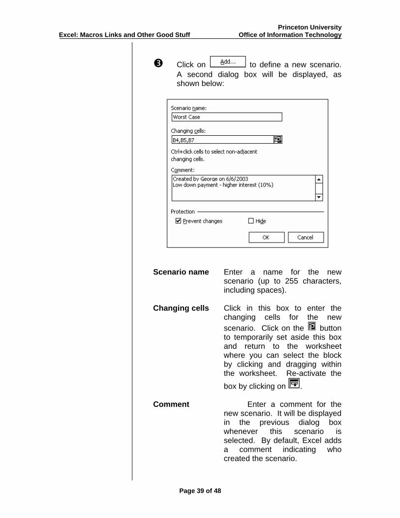
Click on to define a new scenario. A second dialog box will be displayed, as shown below:
Scenario name Enter a name for the new scenario (up to 255 characters, including spaces).
Changing cells Click in this box to enter the
changing cells for the new scenario. Click on the button to temporarily set aside this box and return to the worksheet where you can select the block by clicking and dragging within the worksheet. Re-activate the box by clicking on .
Comment Enter a comment for the
new scenario. It will be displayed in the previous dialog box whenever this scenario is selected. By default, Excel adds a comment indicating who created the scenario.
Page 39 of 48
Princeton University Excel: Macros Links and Other Good Stuff Office of Information Technology
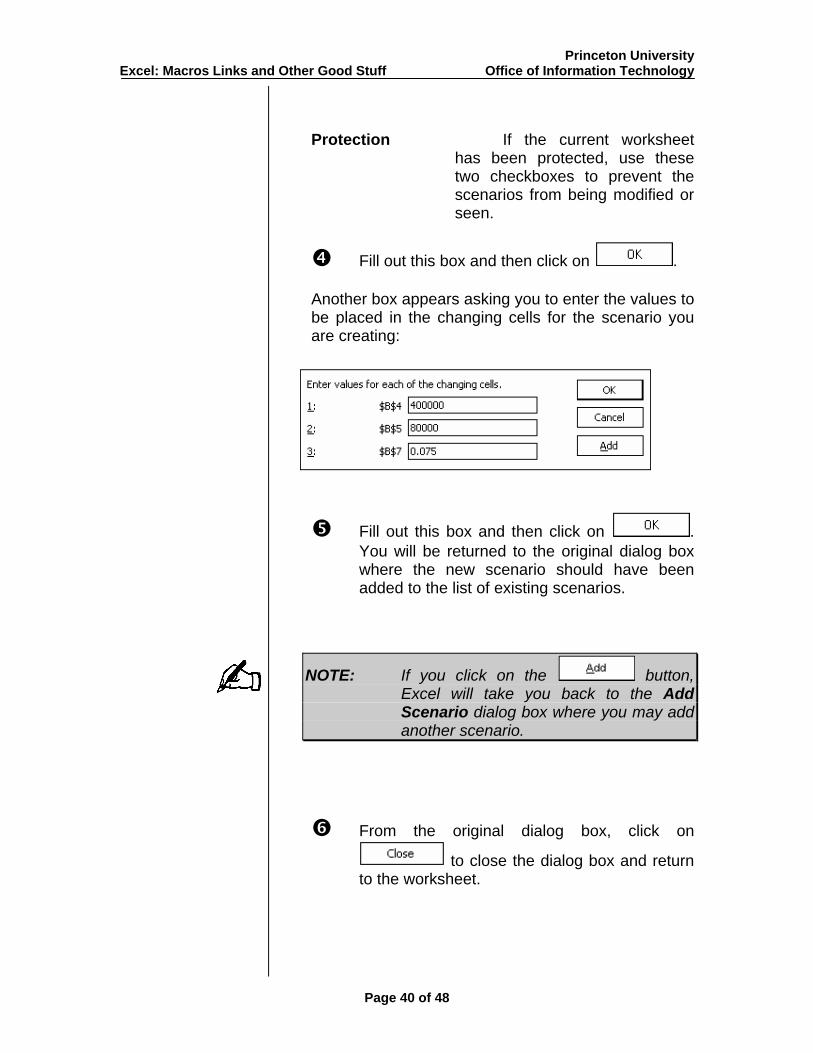
Protection If the current worksheet has been protected, use these two checkboxes to prevent the scenarios from being modified or seen.
Fill out this box and then click on . Another box appears asking you to enter the values to be placed in the changing cells for the scenario you are creating:
Fill out this box and then click on . You will be returned to the original dialog box where the new scenario should have been added to the list of existing scenarios.
NOTE: If you click on the button, Excel will take you back to the Add Scenario dialog box where you may add another scenario.
From the original dialog box, click on
to close the dialog box and return to the worksheet.
Page 40 of 48
Princeton University Excel: Macros Links and Other Good Stuff Office of Information Technology
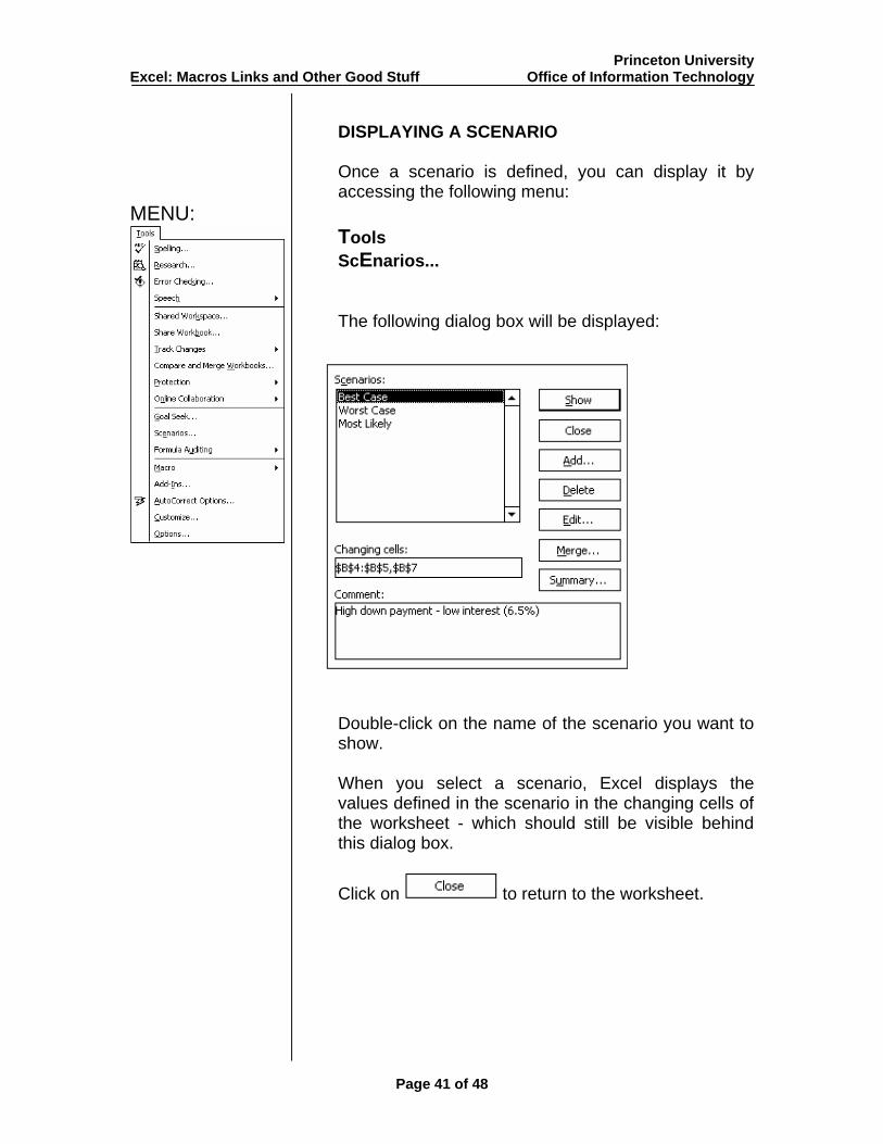
DISPLAYING A SCENARIO
Once a scenario is defined, you can display it by accessing the following menu:
MENU: Tools T
ScEnarios...
The following dialog box will be displayed:
Double-click on the name of the scenario you want to show.
When you select a scenario, Excel displays the values defined in the scenario in the changing cells of the worksheet - which should still be visible behind this dialog box.
Click on to return to the worksheet.
Page 41 of 48
Princeton University Excel: Macros Links and Other Good Stuff Office of Information Technology
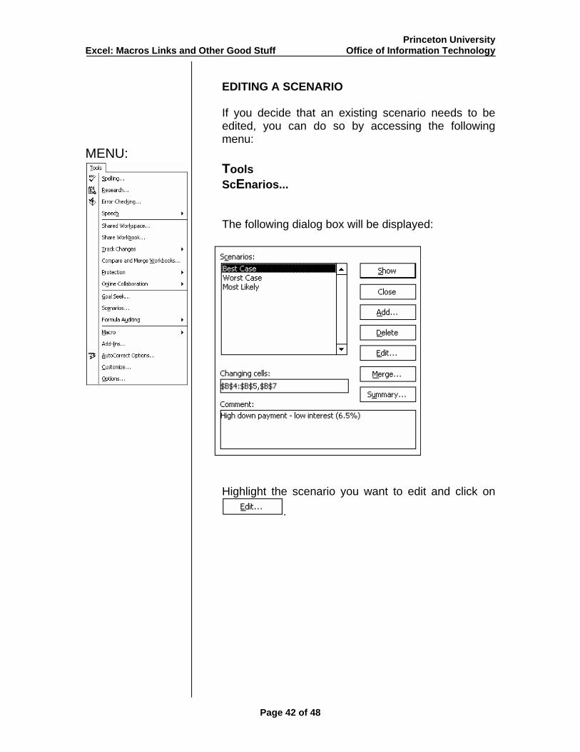
EDITING A SCENARIO
If you decide that an existing scenario needs to be edited, you can do so by accessing the following menu:
MENU: Tools T
ScEnarios...
The following dialog box will be displayed:
Highlight the scenario you want to edit and click on
.
Page 42 of 48
Princeton University Excel: Macros Links and Other Good Stuff Office of Information Technology
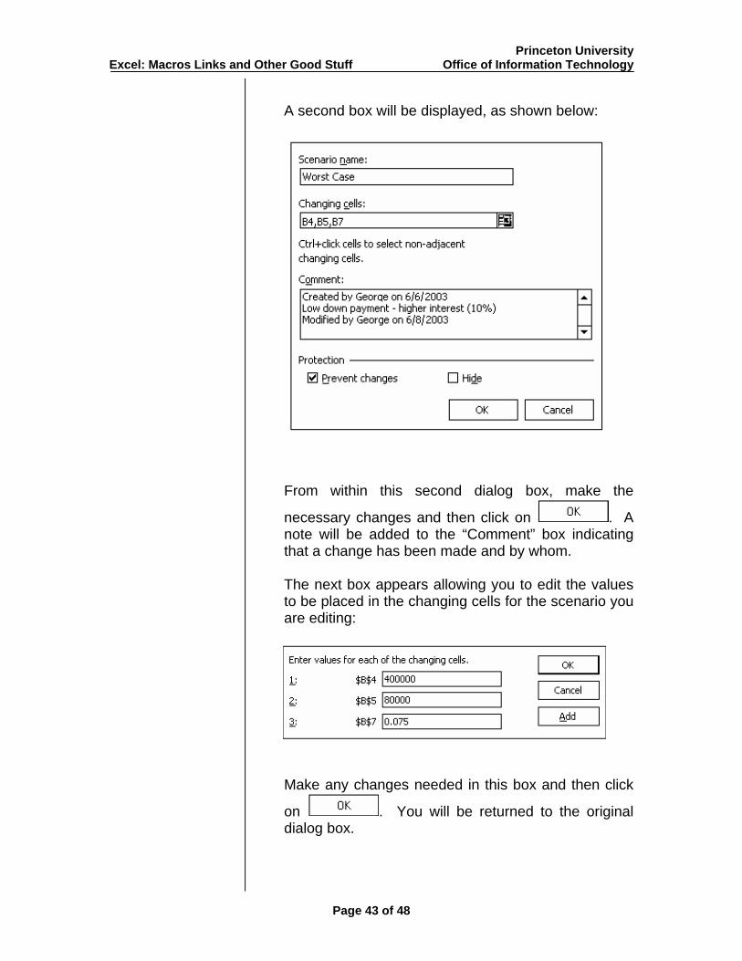
A second box will be displayed, as shown below:
From within this second dialog box, make the
necessary changes and then click on . A note will be added to the “Comment” box indicating that a change has been made and by whom.
The next box appears allowing you to edit the values to be placed in the changing cells for the scenario you are editing:
Make any changes needed in this box and then click
on . You will be returned to the original dialog box.
Page 43 of 48
Princeton University Excel: Macros Links and Other Good Stuff Office of Information Technology
Click on to return to the worksheet.
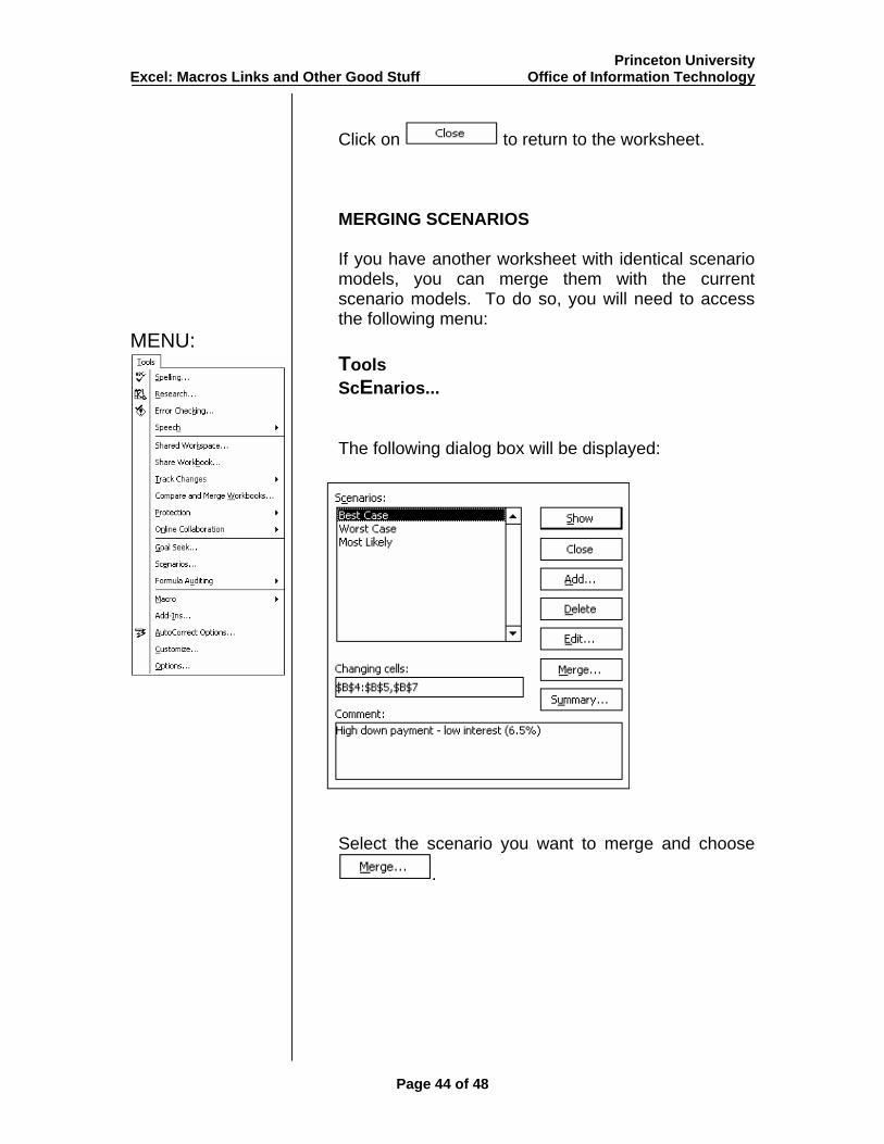
MERGING SCENARIOS
If you have another worksheet with identical scenario models, you can merge them with the current scenario models. To do so, you will need to access the following menu:
MENU: Tools T
ScEnarios...
The following dialog box will be displayed:
Select the scenario you want to merge and choose
.
Page 44 of 48
Princeton University Excel: Macros Links and Other Good Stuff Office of Information Technology
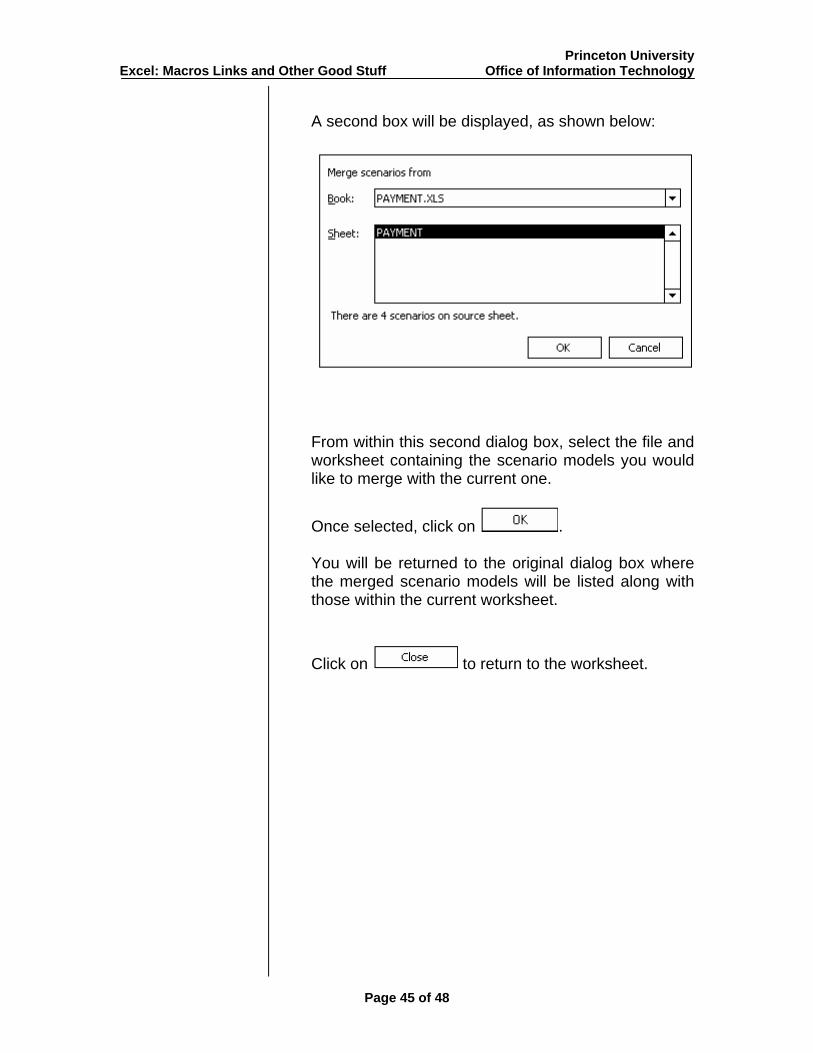
A second box will be displayed, as shown below:
From within this second dialog box, select the file and worksheet containing the scenario models you would like to merge with the current one.
Once selected, click on .
You will be returned to the original dialog box where the merged scenario models will be listed along with those within the current worksheet.
Click on to return to the worksheet.
Page 45 of 48
Princeton University Excel: Macros Links and Other Good Stuff Office of Information Technology
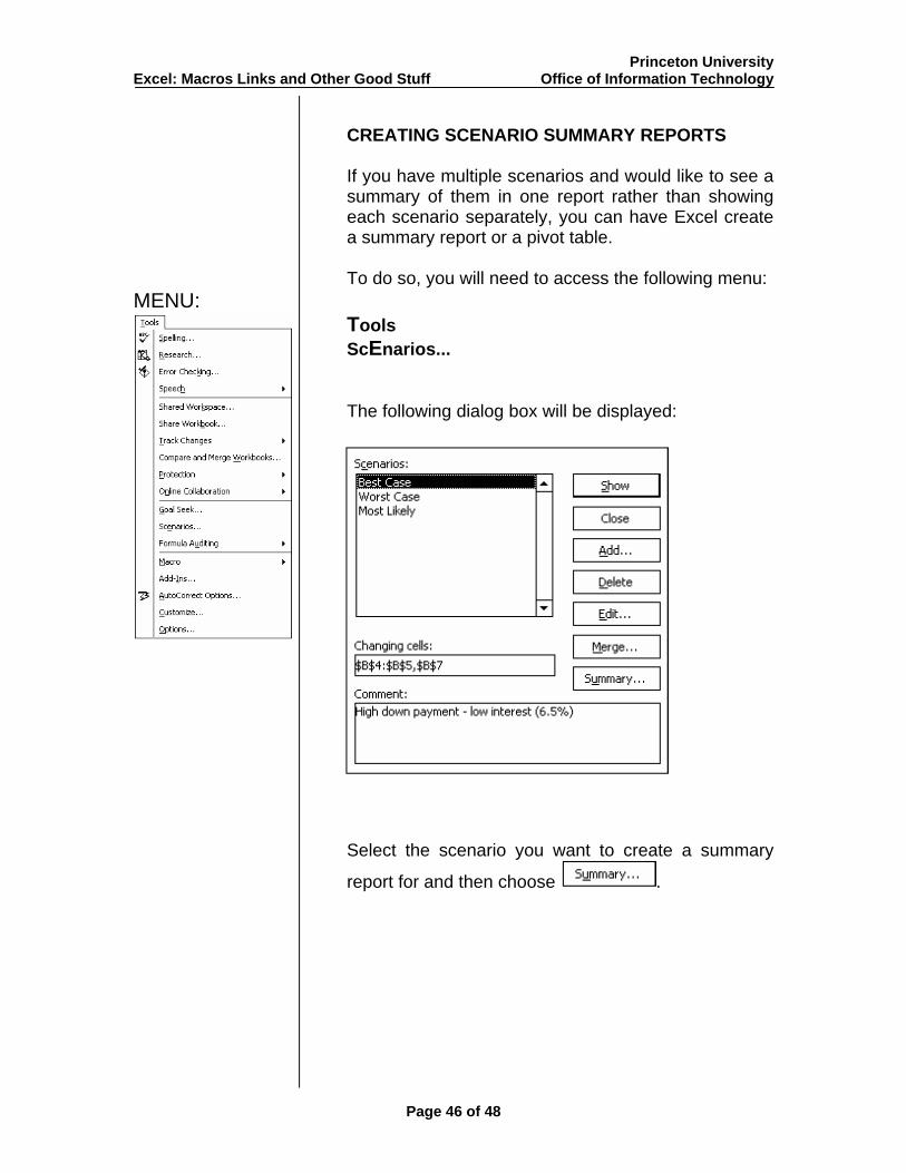
CREATING SCENARIO SUMMARY REPORTS
If you have multiple scenarios and would like to see a summary of them in one report rather than showing each scenario separately, you can have Excel create a summary report or a pivot table.
To do so, you will need to access the following menu:
MENU: Tools T
ScEnarios...
The following dialog box will be displayed:
Select the scenario you want to create a summary
report for and then choose .
Page 46 of 48
Princeton University Excel: Macros Links and Other Good Stuff Office of Information Technology
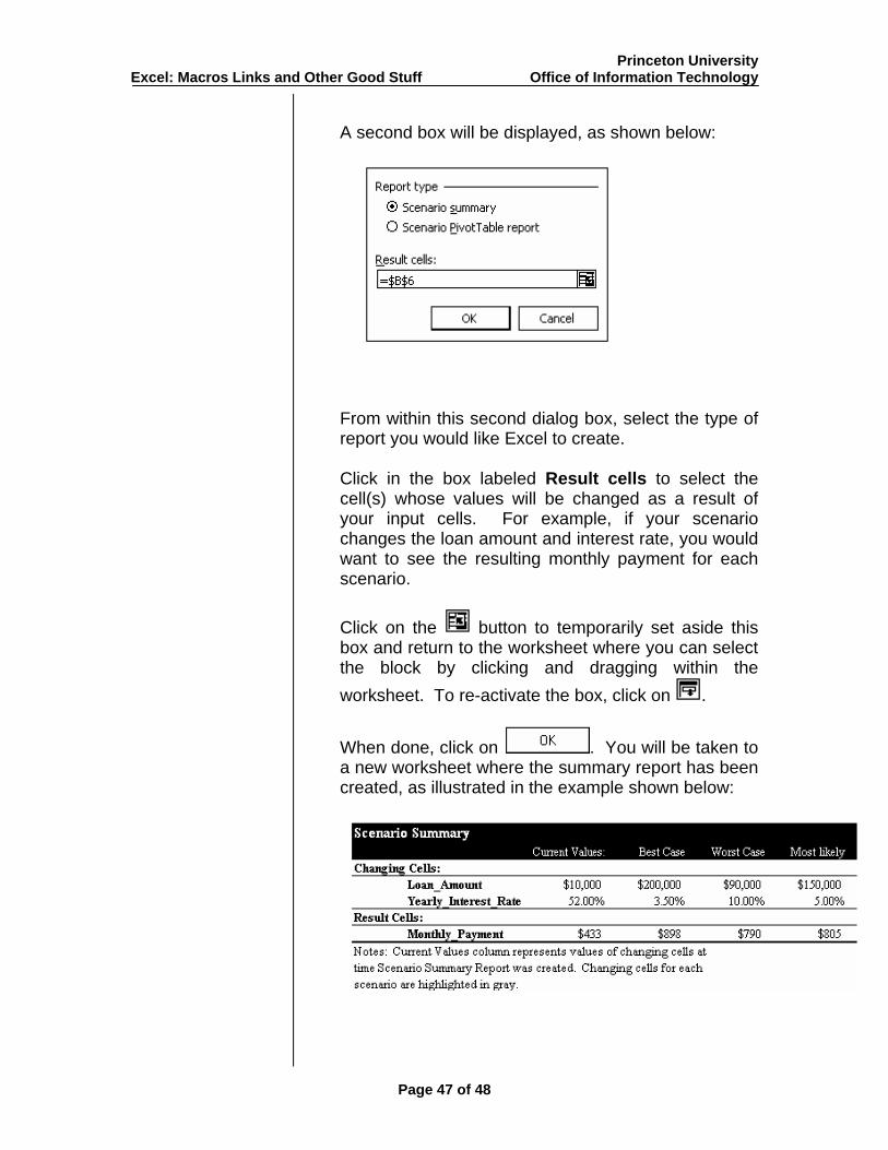
A second box will be displayed, as shown below:
From within this second dialog box, select the type of report you would like Excel to create.
Click in the box labeled Result cells to select the cell(s) whose values will be changed as a result of your input cells. For example, if your scenario changes the loan amount and interest rate, you would want to see the resulting monthly payment for each scenario.
Click on the button to temporarily set aside this box and return to the worksheet where you can select the block by clicking and dragging within the worksheet. To re-activate the box, click on .
When done, click on . You will be taken to a new worksheet where the summary report has been created, as illustrated in the example shown below:
Page 47 of 48
Princeton University Excel: Macros Links and Other Good Stuff Office of Information Technology
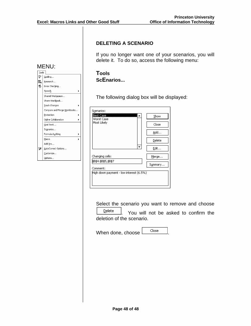
DELETING A SCENARIO
If you no longer want one of your scenarios, you will delete it. To do so, access the following menu:
MENU: Tools T
ScEnarios...
The following dialog box will be displayed:
Select the scenario you want to remove and choose
. You will not be asked to confirm the deletion of the scenario.
When done, choose .
Page 48 of 48