Embed Size (px)
Citation preview

MacroeconomicsSlides 7th lecture
Luis REYES1
Panthéon Sorbonne Master in Economics, Université Paris 1
[email protected] or [email protected], www.luisreyesortiz.orgL. Reyes (Paris 1) Macro 7 11/09/2017 1 / 48

Outline
1 Real Business CyclesIntroductionBusiness cycle phenomena and growth modelUsing data to restrict the growth model, i.e. calibration
2 Dynamic Stochastic General Equilibrium modelsIntroductionThe linearized DSGE modelParameter estimates and model properties
L. Reyes (Paris 1) Macro 7 11/09/2017 2 / 48

Outline
1 Real Business CyclesIntroductionBusiness cycle phenomena and growth modelUsing data to restrict the growth model, i.e. calibration
2 Dynamic Stochastic General Equilibrium modelsIntroductionThe linearized DSGE modelParameter estimates and model properties
L. Reyes (Paris 1) Macro 7 11/09/2017 3 / 48

Outline
1 Real Business CyclesIntroductionBusiness cycle phenomena and growth modelUsing data to restrict the growth model, i.e. calibration
2 Dynamic Stochastic General Equilibrium modelsIntroductionThe linearized DSGE modelParameter estimates and model properties
L. Reyes (Paris 1) Macro 7 11/09/2017 4 / 48

Introduction (1)Prescott (1986)
The first part of today’s lecture is based on Prescott’s article "Theoryahead of business cycle measurement".
This article is part of a research program by (among others) Kydlandand Prescott (1982, 1987), Hansen (1985) and Bain (1985).The authors computed competitive equilibrium stochastic process forvariants of the constant elasticity, stochastic growth model.The elasticities of substitution and the share parameters of theproduction and utility functions are restricted to those that generatethe growth observations.They ask whether these artificial economies display fluctuations withstatistical properties similar to those which the American economyhas displayed since the Korean War.
L. Reyes (Paris 1) Macro 7 11/09/2017 5 / 48

Introduction (1)Prescott (1986)
The first part of today’s lecture is based on Prescott’s article "Theoryahead of business cycle measurement".This article is part of a research program by (among others) Kydlandand Prescott (1982, 1987), Hansen (1985) and Bain (1985).
The authors computed competitive equilibrium stochastic process forvariants of the constant elasticity, stochastic growth model.The elasticities of substitution and the share parameters of theproduction and utility functions are restricted to those that generatethe growth observations.They ask whether these artificial economies display fluctuations withstatistical properties similar to those which the American economyhas displayed since the Korean War.
L. Reyes (Paris 1) Macro 7 11/09/2017 5 / 48

Introduction (1)Prescott (1986)
The first part of today’s lecture is based on Prescott’s article "Theoryahead of business cycle measurement".This article is part of a research program by (among others) Kydlandand Prescott (1982, 1987), Hansen (1985) and Bain (1985).The authors computed competitive equilibrium stochastic process forvariants of the constant elasticity, stochastic growth model.
The elasticities of substitution and the share parameters of theproduction and utility functions are restricted to those that generatethe growth observations.They ask whether these artificial economies display fluctuations withstatistical properties similar to those which the American economyhas displayed since the Korean War.
L. Reyes (Paris 1) Macro 7 11/09/2017 5 / 48

Introduction (1)Prescott (1986)
The first part of today’s lecture is based on Prescott’s article "Theoryahead of business cycle measurement".This article is part of a research program by (among others) Kydlandand Prescott (1982, 1987), Hansen (1985) and Bain (1985).The authors computed competitive equilibrium stochastic process forvariants of the constant elasticity, stochastic growth model.The elasticities of substitution and the share parameters of theproduction and utility functions are restricted to those that generatethe growth observations.
They ask whether these artificial economies display fluctuations withstatistical properties similar to those which the American economyhas displayed since the Korean War.
L. Reyes (Paris 1) Macro 7 11/09/2017 5 / 48

Introduction (1)Prescott (1986)
The first part of today’s lecture is based on Prescott’s article "Theoryahead of business cycle measurement".This article is part of a research program by (among others) Kydlandand Prescott (1982, 1987), Hansen (1985) and Bain (1985).The authors computed competitive equilibrium stochastic process forvariants of the constant elasticity, stochastic growth model.The elasticities of substitution and the share parameters of theproduction and utility functions are restricted to those that generatethe growth observations.They ask whether these artificial economies display fluctuations withstatistical properties similar to those which the American economyhas displayed since the Korean War.
L. Reyes (Paris 1) Macro 7 11/09/2017 5 / 48

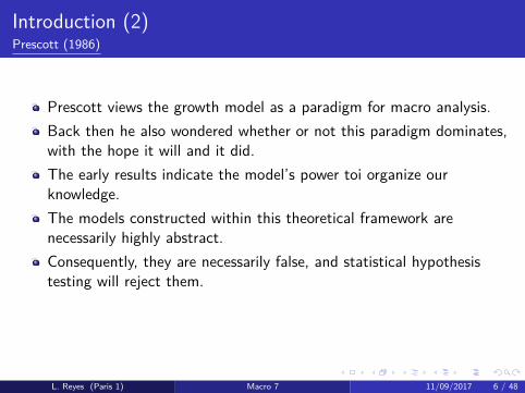
Introduction (2)Prescott (1986)
Prescott views the growth model as a paradigm for macro analysis.
Back then he also wondered whether or not this paradigm dominates,with the hope it will
and it did.The early results indicate the model’s power toi organize ourknowledge.The models constructed within this theoretical framework arenecessarily highly abstract.Consequently, they are necessarily false, and statistical hypothesistesting will reject them.The research reviewed in this article is best viewed as a verypromising beginning of a much larger research program.
L. Reyes (Paris 1) Macro 7 11/09/2017 6 / 48

Introduction (2)Prescott (1986)
Prescott views the growth model as a paradigm for macro analysis.Back then he also wondered whether or not this paradigm dominates,with the hope it will
and it did.
The early results indicate the model’s power toi organize ourknowledge.The models constructed within this theoretical framework arenecessarily highly abstract.Consequently, they are necessarily false, and statistical hypothesistesting will reject them.The research reviewed in this article is best viewed as a verypromising beginning of a much larger research program.
L. Reyes (Paris 1) Macro 7 11/09/2017 6 / 48

Introduction (2)Prescott (1986)
Prescott views the growth model as a paradigm for macro analysis.Back then he also wondered whether or not this paradigm dominates,with the hope it will and it did.
The early results indicate the model’s power toi organize ourknowledge.The models constructed within this theoretical framework arenecessarily highly abstract.Consequently, they are necessarily false, and statistical hypothesistesting will reject them.The research reviewed in this article is best viewed as a verypromising beginning of a much larger research program.
L. Reyes (Paris 1) Macro 7 11/09/2017 6 / 48

Introduction (2)Prescott (1986)
Prescott views the growth model as a paradigm for macro analysis.Back then he also wondered whether or not this paradigm dominates,with the hope it will and it did.The early results indicate the model’s power toi organize ourknowledge.
The models constructed within this theoretical framework arenecessarily highly abstract.Consequently, they are necessarily false, and statistical hypothesistesting will reject them.The research reviewed in this article is best viewed as a verypromising beginning of a much larger research program.
L. Reyes (Paris 1) Macro 7 11/09/2017 6 / 48

Introduction (2)Prescott (1986)
Prescott views the growth model as a paradigm for macro analysis.Back then he also wondered whether or not this paradigm dominates,with the hope it will and it did.The early results indicate the model’s power toi organize ourknowledge.The models constructed within this theoretical framework arenecessarily highly abstract.
Consequently, they are necessarily false, and statistical hypothesistesting will reject them.The research reviewed in this article is best viewed as a verypromising beginning of a much larger research program.
L. Reyes (Paris 1) Macro 7 11/09/2017 6 / 48
Introduction (2)Prescott (1986)
Prescott views the growth model as a paradigm for macro analysis.Back then he also wondered whether or not this paradigm dominates,with the hope it will and it did.The early results indicate the model’s power toi organize ourknowledge.The models constructed within this theoretical framework arenecessarily highly abstract.Consequently, they are necessarily false, and statistical hypothesistesting will reject them.
The research reviewed in this article is best viewed as a verypromising beginning of a much larger research program.
L. Reyes (Paris 1) Macro 7 11/09/2017 6 / 48

Introduction (2)Prescott (1986)
Prescott views the growth model as a paradigm for macro analysis.Back then he also wondered whether or not this paradigm dominates,with the hope it will and it did.The early results indicate the model’s power toi organize ourknowledge.The models constructed within this theoretical framework arenecessarily highly abstract.Consequently, they are necessarily false, and statistical hypothesistesting will reject them.The research reviewed in this article is best viewed as a verypromising beginning of a much larger research program.
L. Reyes (Paris 1) Macro 7 11/09/2017 6 / 48

Outline
1 Real Business CyclesIntroductionBusiness cycle phenomena and growth modelUsing data to restrict the growth model, i.e. calibration
2 Dynamic Stochastic General Equilibrium modelsIntroductionThe linearized DSGE modelParameter estimates and model properties
L. Reyes (Paris 1) Macro 7 11/09/2017 7 / 48

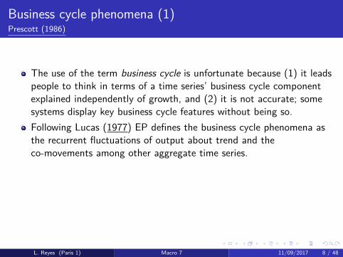
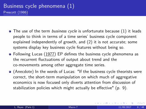
Business cycle phenomena (1)Prescott (1986)
The use of the term business cycle is unfortunate because
(1) it leadspeople to think in terms of a time series’ business cycle componentexplained independently of growth, and (2) it is not accurate; somesystems display key business cycle features without being so.
Following Lucas (1977) EP defines the business cycle phenomena asthe recurrent fluctuations of output about trend and theco-movements among other aggregate time series.(Anecdote) In the words of Lucas: "If the business cycle theorists werecorrect, the short-term manipulation on which much of aggregativeeconomics is now focused only diverts attention from discussion ofstabilization policies which might actually be effective" (p. 9).
L. Reyes (Paris 1) Macro 7 11/09/2017 8 / 48

Business cycle phenomena (1)Prescott (1986)
The use of the term business cycle is unfortunate because (1) it leadspeople to think in terms of a time series’ business cycle componentexplained independently of growth, and
(2) it is not accurate; somesystems display key business cycle features without being so.
Following Lucas (1977) EP defines the business cycle phenomena asthe recurrent fluctuations of output about trend and theco-movements among other aggregate time series.(Anecdote) In the words of Lucas: "If the business cycle theorists werecorrect, the short-term manipulation on which much of aggregativeeconomics is now focused only diverts attention from discussion ofstabilization policies which might actually be effective" (p. 9).
L. Reyes (Paris 1) Macro 7 11/09/2017 8 / 48

Business cycle phenomena (1)Prescott (1986)
The use of the term business cycle is unfortunate because (1) it leadspeople to think in terms of a time series’ business cycle componentexplained independently of growth, and (2) it is not accurate; somesystems display key business cycle features without being so.
Following Lucas (1977) EP defines the business cycle phenomena asthe recurrent fluctuations of output about trend and theco-movements among other aggregate time series.(Anecdote) In the words of Lucas: "If the business cycle theorists werecorrect, the short-term manipulation on which much of aggregativeeconomics is now focused only diverts attention from discussion ofstabilization policies which might actually be effective" (p. 9).
L. Reyes (Paris 1) Macro 7 11/09/2017 8 / 48
Business cycle phenomena (1)Prescott (1986)
The use of the term business cycle is unfortunate because (1) it leadspeople to think in terms of a time series’ business cycle componentexplained independently of growth, and (2) it is not accurate; somesystems display key business cycle features without being so.Following Lucas (1977) EP defines the business cycle phenomena asthe recurrent fluctuations of output about trend and theco-movements among other aggregate time series.
(Anecdote) In the words of Lucas: "If the business cycle theorists werecorrect, the short-term manipulation on which much of aggregativeeconomics is now focused only diverts attention from discussion ofstabilization policies which might actually be effective" (p. 9).
L. Reyes (Paris 1) Macro 7 11/09/2017 8 / 48
Business cycle phenomena (1)Prescott (1986)
The use of the term business cycle is unfortunate because (1) it leadspeople to think in terms of a time series’ business cycle componentexplained independently of growth, and (2) it is not accurate; somesystems display key business cycle features without being so.Following Lucas (1977) EP defines the business cycle phenomena asthe recurrent fluctuations of output about trend and theco-movements among other aggregate time series.(Anecdote) In the words of Lucas: "If the business cycle theorists werecorrect, the short-term manipulation on which much of aggregativeeconomics is now focused only diverts attention from discussion ofstabilization policies which might actually be effective" (p. 9).
L. Reyes (Paris 1) Macro 7 11/09/2017 8 / 48

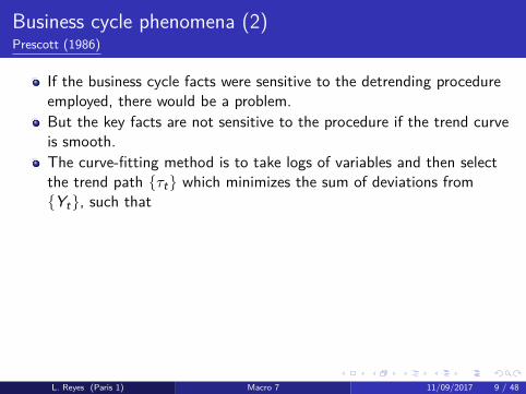
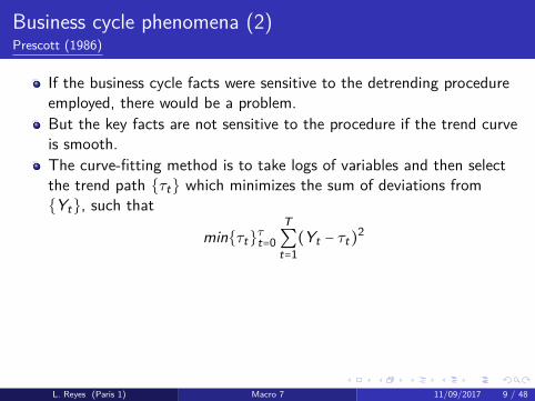
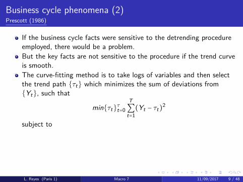
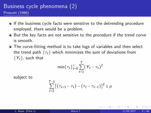
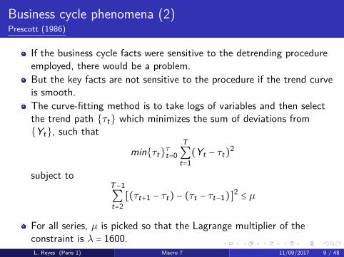
Business cycle phenomena (2)Prescott (1986)
If the business cycle facts were sensitive to the detrending procedureemployed, there would be a problem.
But the key facts are not sensitive to the procedure if the trend curveis smooth.The curve-fitting method is to take logs of variables and then selectthe trend path {τt} which minimizes the sum of deviations from{Yt}, such that
min{τt}τt=0
T∑t=1
(Yt − τt)2
subject toT−1∑t=2
[(τt+1 − τt) − (τt − τt−1)]2≤ µ
For all series, µ is picked so that the Lagrange multiplier of theconstraint is λ = 1600.
L. Reyes (Paris 1) Macro 7 11/09/2017 9 / 48

Business cycle phenomena (2)Prescott (1986)
If the business cycle facts were sensitive to the detrending procedureemployed, there would be a problem.But the key facts are not sensitive to the procedure if the trend curveis smooth.
The curve-fitting method is to take logs of variables and then selectthe trend path {τt} which minimizes the sum of deviations from{Yt}, such that
min{τt}τt=0
T∑t=1
(Yt − τt)2
subject toT−1∑t=2
[(τt+1 − τt) − (τt − τt−1)]2≤ µ
For all series, µ is picked so that the Lagrange multiplier of theconstraint is λ = 1600.
L. Reyes (Paris 1) Macro 7 11/09/2017 9 / 48

Business cycle phenomena (2)Prescott (1986)
If the business cycle facts were sensitive to the detrending procedureemployed, there would be a problem.But the key facts are not sensitive to the procedure if the trend curveis smooth.The curve-fitting method is to take logs of variables and then selectthe trend path {τt} which minimizes the sum of deviations from{Yt}, such that
min{τt}τt=0
T∑t=1
(Yt − τt)2
subject toT−1∑t=2
[(τt+1 − τt) − (τt − τt−1)]2≤ µ
For all series, µ is picked so that the Lagrange multiplier of theconstraint is λ = 1600.
L. Reyes (Paris 1) Macro 7 11/09/2017 9 / 48
Business cycle phenomena (2)Prescott (1986)
If the business cycle facts were sensitive to the detrending procedureemployed, there would be a problem.But the key facts are not sensitive to the procedure if the trend curveis smooth.The curve-fitting method is to take logs of variables and then selectthe trend path {τt} which minimizes the sum of deviations from{Yt}, such that
min{τt}τt=0
T∑t=1
(Yt − τt)2
subject to
T−1∑t=2
[(τt+1 − τt) − (τt − τt−1)]2≤ µ
For all series, µ is picked so that the Lagrange multiplier of theconstraint is λ = 1600.
L. Reyes (Paris 1) Macro 7 11/09/2017 9 / 48
Business cycle phenomena (2)Prescott (1986)
If the business cycle facts were sensitive to the detrending procedureemployed, there would be a problem.But the key facts are not sensitive to the procedure if the trend curveis smooth.The curve-fitting method is to take logs of variables and then selectthe trend path {τt} which minimizes the sum of deviations from{Yt}, such that
min{τt}τt=0
T∑t=1
(Yt − τt)2
subject toT−1∑t=2
[(τt+1 − τt) − (τt − τt−1)]2≤ µ
For all series, µ is picked so that the Lagrange multiplier of theconstraint is λ = 1600.
L. Reyes (Paris 1) Macro 7 11/09/2017 9 / 48
Business cycle phenomena (2)Prescott (1986)
If the business cycle facts were sensitive to the detrending procedureemployed, there would be a problem.But the key facts are not sensitive to the procedure if the trend curveis smooth.The curve-fitting method is to take logs of variables and then selectthe trend path {τt} which minimizes the sum of deviations from{Yt}, such that
min{τt}τt=0
T∑t=1
(Yt − τt)2
subject toT−1∑t=2
[(τt+1 − τt) − (τt − τt−1)]2≤ µ
For all series, µ is picked so that the Lagrange multiplier of theconstraint is λ = 1600.L. Reyes (Paris 1) Macro 7 11/09/2017 9 / 48

Business cycle phenomena (2’)Parenthesis
Today this procedure is known as the H-P filter, and is widely used inthe economic literature.
However, it should be rather called the Whittaker-Hendersongraduation method (see MacCaulay, 1931).This method is used to decompose economic data into a trend and acyclical component, so that the larger the value of λ the smootherthe resulting filtered series.But the choice of λ is arbitrary (de Alba and Gómez, 2012; Hamilton2016).Not so long ago, the usefulness of the H-P filter was (and still is!) amatter of lively debate.Among others because some people use the HP filtered GDP to arguethat the US economy is already operating near potential, so thatthere is no reason to pursue expansionary policy (Krugman).
L. Reyes (Paris 1) Macro 7 11/09/2017 10 / 48

Business cycle phenomena (2’)Parenthesis
Today this procedure is known as the H-P filter, and is widely used inthe economic literature.However, it should be rather called the Whittaker-Hendersongraduation method (see MacCaulay, 1931).
This method is used to decompose economic data into a trend and acyclical component, so that the larger the value of λ the smootherthe resulting filtered series.But the choice of λ is arbitrary (de Alba and Gómez, 2012; Hamilton2016).Not so long ago, the usefulness of the H-P filter was (and still is!) amatter of lively debate.Among others because some people use the HP filtered GDP to arguethat the US economy is already operating near potential, so thatthere is no reason to pursue expansionary policy (Krugman).
L. Reyes (Paris 1) Macro 7 11/09/2017 10 / 48

Business cycle phenomena (2’)Parenthesis
Today this procedure is known as the H-P filter, and is widely used inthe economic literature.However, it should be rather called the Whittaker-Hendersongraduation method (see MacCaulay, 1931).This method is used to decompose economic data into a trend and acyclical component, so that the larger the value of λ the smootherthe resulting filtered series.
But the choice of λ is arbitrary (de Alba and Gómez, 2012; Hamilton2016).Not so long ago, the usefulness of the H-P filter was (and still is!) amatter of lively debate.Among others because some people use the HP filtered GDP to arguethat the US economy is already operating near potential, so thatthere is no reason to pursue expansionary policy (Krugman).
L. Reyes (Paris 1) Macro 7 11/09/2017 10 / 48

Business cycle phenomena (2’)Parenthesis
Today this procedure is known as the H-P filter, and is widely used inthe economic literature.However, it should be rather called the Whittaker-Hendersongraduation method (see MacCaulay, 1931).This method is used to decompose economic data into a trend and acyclical component, so that the larger the value of λ the smootherthe resulting filtered series.But the choice of λ is arbitrary (de Alba and Gómez, 2012; Hamilton2016).
Not so long ago, the usefulness of the H-P filter was (and still is!) amatter of lively debate.Among others because some people use the HP filtered GDP to arguethat the US economy is already operating near potential, so thatthere is no reason to pursue expansionary policy (Krugman).
L. Reyes (Paris 1) Macro 7 11/09/2017 10 / 48

Business cycle phenomena (2’)Parenthesis
Today this procedure is known as the H-P filter, and is widely used inthe economic literature.However, it should be rather called the Whittaker-Hendersongraduation method (see MacCaulay, 1931).This method is used to decompose economic data into a trend and acyclical component, so that the larger the value of λ the smootherthe resulting filtered series.But the choice of λ is arbitrary (de Alba and Gómez, 2012; Hamilton2016).Not so long ago, the usefulness of the H-P filter was (and still is!) amatter of lively debate.
Among others because some people use the HP filtered GDP to arguethat the US economy is already operating near potential, so thatthere is no reason to pursue expansionary policy (Krugman).
L. Reyes (Paris 1) Macro 7 11/09/2017 10 / 48

Business cycle phenomena (2’)Parenthesis
Today this procedure is known as the H-P filter, and is widely used inthe economic literature.However, it should be rather called the Whittaker-Hendersongraduation method (see MacCaulay, 1931).This method is used to decompose economic data into a trend and acyclical component, so that the larger the value of λ the smootherthe resulting filtered series.But the choice of λ is arbitrary (de Alba and Gómez, 2012; Hamilton2016).Not so long ago, the usefulness of the H-P filter was (and still is!) amatter of lively debate.Among others because some people use the HP filtered GDP to arguethat the US economy is already operating near potential, so thatthere is no reason to pursue expansionary policy (Krugman).
L. Reyes (Paris 1) Macro 7 11/09/2017 10 / 48

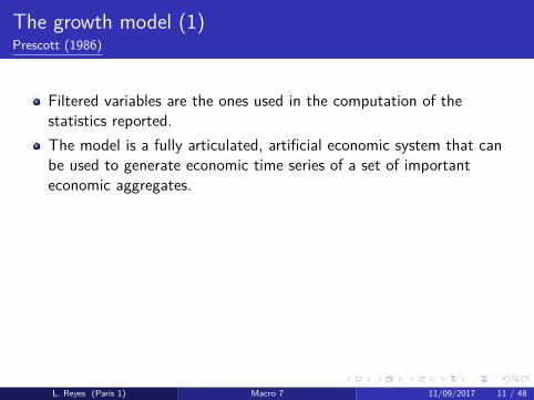
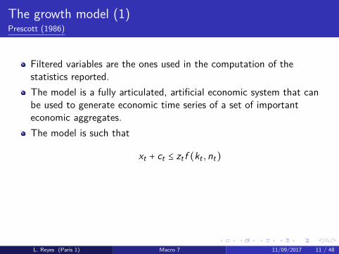
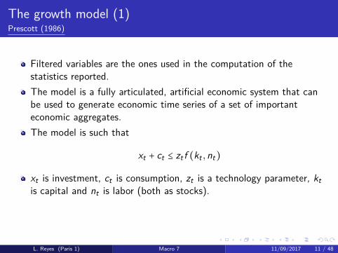
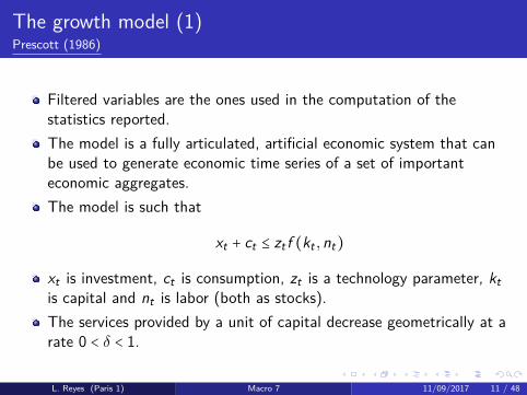
The growth model (1)Prescott (1986)
Filtered variables are the ones used in the computation of thestatistics reported.
The model is a fully articulated, artificial economic system that canbe used to generate economic time series of a set of importanteconomic aggregates.The model is such that
xt + ct ≤ zt f (kt ,nt)
xt is investment, ct is consumption, zt is a technology parameter, ktis capital and nt is labor (both as stocks).The services provided by a unit of capital decrease geometrically at arate 0 < δ < 1.
L. Reyes (Paris 1) Macro 7 11/09/2017 11 / 48
The growth model (1)Prescott (1986)
Filtered variables are the ones used in the computation of thestatistics reported.The model is a fully articulated, artificial economic system that canbe used to generate economic time series of a set of importanteconomic aggregates.
The model is such that
xt + ct ≤ zt f (kt ,nt)
xt is investment, ct is consumption, zt is a technology parameter, ktis capital and nt is labor (both as stocks).The services provided by a unit of capital decrease geometrically at arate 0 < δ < 1.
L. Reyes (Paris 1) Macro 7 11/09/2017 11 / 48
The growth model (1)Prescott (1986)
Filtered variables are the ones used in the computation of thestatistics reported.The model is a fully articulated, artificial economic system that canbe used to generate economic time series of a set of importanteconomic aggregates.The model is such that
xt + ct ≤ zt f (kt ,nt)
xt is investment, ct is consumption, zt is a technology parameter, ktis capital and nt is labor (both as stocks).
The services provided by a unit of capital decrease geometrically at arate 0 < δ < 1.
L. Reyes (Paris 1) Macro 7 11/09/2017 11 / 48
The growth model (1)Prescott (1986)
Filtered variables are the ones used in the computation of thestatistics reported.The model is a fully articulated, artificial economic system that canbe used to generate economic time series of a set of importanteconomic aggregates.The model is such that
xt + ct ≤ zt f (kt ,nt)
xt is investment, ct is consumption, zt is a technology parameter, ktis capital and nt is labor (both as stocks).The services provided by a unit of capital decrease geometrically at arate 0 < δ < 1.
L. Reyes (Paris 1) Macro 7 11/09/2017 11 / 48
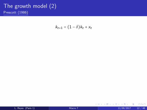
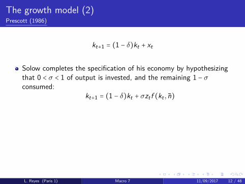
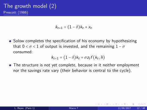
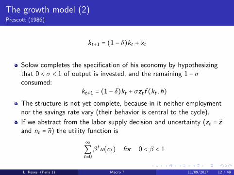
The growth model (2)Prescott (1986)
kt+1 = (1 − δ)kt + xt
Solow completes the specification of his economy by hypothesizingthat 0 < σ < 1 of output is invested, and the remaining 1 − σconsumed:
kt+1 = (1 − δ)kt + σzt f (kt , n)The structure is not yet complete, because in it neither employmentnor the savings rate vary (their behavior is central to the cycle).If we abstract from the labor supply decision and uncertainty (zt = zand nt = n) the utility function is
∞∑t=0βtu(ct) for 0 < β < 1
L. Reyes (Paris 1) Macro 7 11/09/2017 12 / 48
The growth model (2)Prescott (1986)
kt+1 = (1 − δ)kt + xt
Solow completes the specification of his economy by hypothesizingthat 0 < σ < 1 of output is invested, and the remaining 1 − σconsumed:
kt+1 = (1 − δ)kt + σzt f (kt , n)
The structure is not yet complete, because in it neither employmentnor the savings rate vary (their behavior is central to the cycle).If we abstract from the labor supply decision and uncertainty (zt = zand nt = n) the utility function is
∞∑t=0βtu(ct) for 0 < β < 1
L. Reyes (Paris 1) Macro 7 11/09/2017 12 / 48
The growth model (2)Prescott (1986)
kt+1 = (1 − δ)kt + xt
Solow completes the specification of his economy by hypothesizingthat 0 < σ < 1 of output is invested, and the remaining 1 − σconsumed:
kt+1 = (1 − δ)kt + σzt f (kt , n)The structure is not yet complete, because in it neither employmentnor the savings rate vary (their behavior is central to the cycle).
If we abstract from the labor supply decision and uncertainty (zt = zand nt = n) the utility function is
∞∑t=0βtu(ct) for 0 < β < 1
L. Reyes (Paris 1) Macro 7 11/09/2017 12 / 48
The growth model (2)Prescott (1986)
kt+1 = (1 − δ)kt + xt
Solow completes the specification of his economy by hypothesizingthat 0 < σ < 1 of output is invested, and the remaining 1 − σconsumed:
kt+1 = (1 − δ)kt + σzt f (kt , n)The structure is not yet complete, because in it neither employmentnor the savings rate vary (their behavior is central to the cycle).If we abstract from the labor supply decision and uncertainty (zt = zand nt = n) the utility function is
∞∑t=0βtu(ct) for 0 < β < 1
L. Reyes (Paris 1) Macro 7 11/09/2017 12 / 48

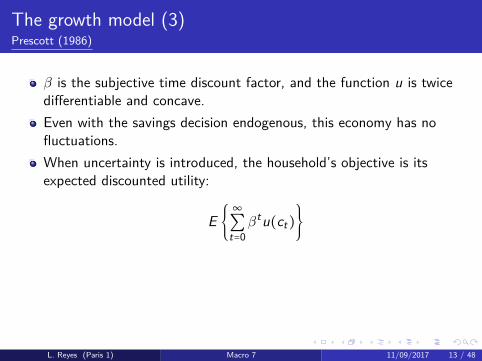
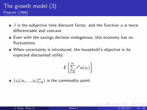
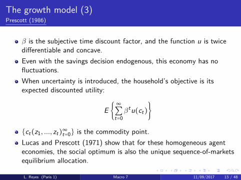
The growth model (3)Prescott (1986)
β is the subjective time discount factor, and the function u is twicedifferentiable and concave.
Even with the savings decision endogenous, this economy has nofluctuations.When uncertainty is introduced, the household’s objective is itsexpected discounted utility:
E {∞∑t=0βtu(ct)}
{ct(z1, ..., zt)∞t=0} is the commodity point.
Lucas and Prescott (1971) show that for these homogeneous agenteconomies, the social optimum is also the unique sequence-of-marketsequilibrium allocation.
L. Reyes (Paris 1) Macro 7 11/09/2017 13 / 48

The growth model (3)Prescott (1986)
β is the subjective time discount factor, and the function u is twicedifferentiable and concave.Even with the savings decision endogenous, this economy has nofluctuations.
When uncertainty is introduced, the household’s objective is itsexpected discounted utility:
E {∞∑t=0βtu(ct)}
{ct(z1, ..., zt)∞t=0} is the commodity point.
Lucas and Prescott (1971) show that for these homogeneous agenteconomies, the social optimum is also the unique sequence-of-marketsequilibrium allocation.
L. Reyes (Paris 1) Macro 7 11/09/2017 13 / 48
The growth model (3)Prescott (1986)
β is the subjective time discount factor, and the function u is twicedifferentiable and concave.Even with the savings decision endogenous, this economy has nofluctuations.When uncertainty is introduced, the household’s objective is itsexpected discounted utility:
E {∞∑t=0βtu(ct)}
{ct(z1, ..., zt)∞t=0} is the commodity point.
Lucas and Prescott (1971) show that for these homogeneous agenteconomies, the social optimum is also the unique sequence-of-marketsequilibrium allocation.
L. Reyes (Paris 1) Macro 7 11/09/2017 13 / 48
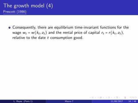
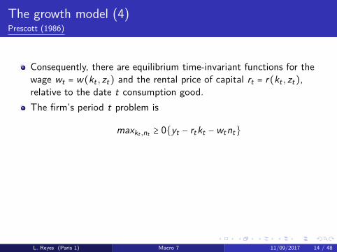
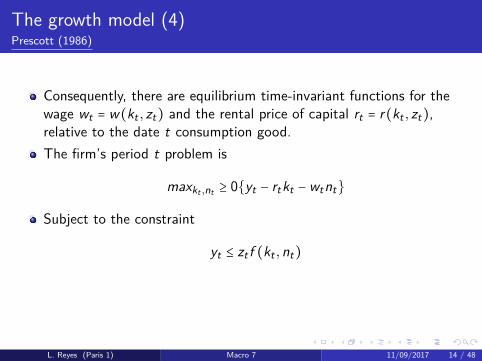
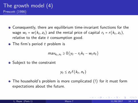
The growth model (4)Prescott (1986)
Consequently, there are equilibrium time-invariant functions for thewage wt = w(kt , zt) and the rental price of capital rt = r(kt , zt),relative to the date t consumption good.
The firm’s period t problem is
maxkt ,nt ≥ 0{yt − rtkt −wtnt}
Subject to the constraint
yt ≤ zt f (kt ,nt)
The household’s problem is more complicated (!) for it must formexpectations about the future.
L. Reyes (Paris 1) Macro 7 11/09/2017 14 / 48
The growth model (4)Prescott (1986)
Consequently, there are equilibrium time-invariant functions for thewage wt = w(kt , zt) and the rental price of capital rt = r(kt , zt),relative to the date t consumption good.The firm’s period t problem is
maxkt ,nt ≥ 0{yt − rtkt −wtnt}
Subject to the constraint
yt ≤ zt f (kt ,nt)
The household’s problem is more complicated (!) for it must formexpectations about the future.
L. Reyes (Paris 1) Macro 7 11/09/2017 14 / 48
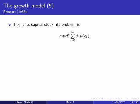
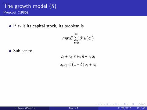
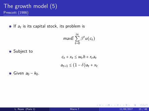
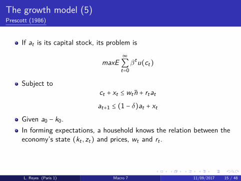
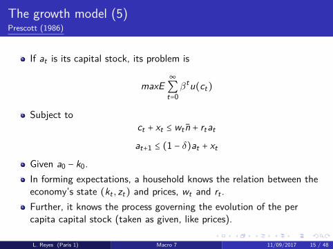
The growth model (5)Prescott (1986)
If at is its capital stock, its problem is
maxE∞∑t=0βtu(ct)
Subject toct + xt ≤ wt n + rtat
at+1 ≤ (1 − δ)at + xt
Given a0 − k0.In forming expectations, a household knows the relation between theeconomy’s state (kt , zt) and prices, wt and rt .Further, it knows the process governing the evolution of the percapita capital stock (taken as given, like prices).
L. Reyes (Paris 1) Macro 7 11/09/2017 15 / 48
The growth model (5)Prescott (1986)
If at is its capital stock, its problem is
maxE∞∑t=0βtu(ct)
Subject toct + xt ≤ wt n + rtat
at+1 ≤ (1 − δ)at + xt
Given a0 − k0.
In forming expectations, a household knows the relation between theeconomy’s state (kt , zt) and prices, wt and rt .Further, it knows the process governing the evolution of the percapita capital stock (taken as given, like prices).
L. Reyes (Paris 1) Macro 7 11/09/2017 15 / 48
The growth model (5)Prescott (1986)
If at is its capital stock, its problem is
maxE∞∑t=0βtu(ct)
Subject toct + xt ≤ wt n + rtat
at+1 ≤ (1 − δ)at + xt
Given a0 − k0.In forming expectations, a household knows the relation between theeconomy’s state (kt , zt) and prices, wt and rt .
Further, it knows the process governing the evolution of the percapita capital stock (taken as given, like prices).
L. Reyes (Paris 1) Macro 7 11/09/2017 15 / 48
The growth model (5)Prescott (1986)
If at is its capital stock, its problem is
maxE∞∑t=0βtu(ct)
Subject toct + xt ≤ wt n + rtat
at+1 ≤ (1 − δ)at + xt
Given a0 − k0.In forming expectations, a household knows the relation between theeconomy’s state (kt , zt) and prices, wt and rt .Further, it knows the process governing the evolution of the percapita capital stock (taken as given, like prices).
L. Reyes (Paris 1) Macro 7 11/09/2017 15 / 48

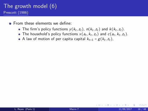
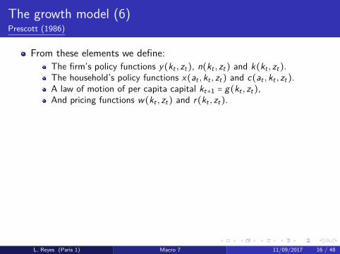
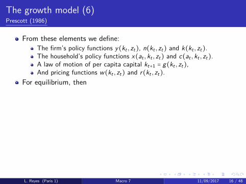
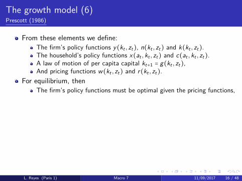
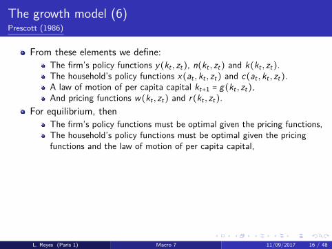
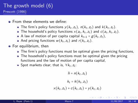
The growth model (6)Prescott (1986)
From these elements we define:
The firm’s policy functions y(kt , zt), n(kt , zt) and k(kt , zt).The household’s policy functions x(at , kt , zt) and c(at , kt , zt).A law of motion of per capita capital kt+1 = g(kt , zt),And pricing functions w(kt , zt) and r(kt , zt).
For equilibrium, then
The firm’s policy functions must be optimal given the pricing functions,The household’s policy functions must be optimal given the pricingfunctions and the law of motion of per capita capital,Spot markets clear; that is, ∀kt , zt :
n = n(kt , zt)
kt = k(kt , zt)
x(kt , zt) + c(kt , zt) = y(kt , zt)
L. Reyes (Paris 1) Macro 7 11/09/2017 16 / 48
The growth model (6)Prescott (1986)
From these elements we define:The firm’s policy functions y(kt , zt), n(kt , zt) and k(kt , zt).
The household’s policy functions x(at , kt , zt) and c(at , kt , zt).A law of motion of per capita capital kt+1 = g(kt , zt),And pricing functions w(kt , zt) and r(kt , zt).
For equilibrium, then
The firm’s policy functions must be optimal given the pricing functions,The household’s policy functions must be optimal given the pricingfunctions and the law of motion of per capita capital,Spot markets clear; that is, ∀kt , zt :
n = n(kt , zt)
kt = k(kt , zt)
x(kt , zt) + c(kt , zt) = y(kt , zt)
L. Reyes (Paris 1) Macro 7 11/09/2017 16 / 48
The growth model (6)Prescott (1986)
From these elements we define:The firm’s policy functions y(kt , zt), n(kt , zt) and k(kt , zt).The household’s policy functions x(at , kt , zt) and c(at , kt , zt).
A law of motion of per capita capital kt+1 = g(kt , zt),And pricing functions w(kt , zt) and r(kt , zt).
For equilibrium, then
The firm’s policy functions must be optimal given the pricing functions,The household’s policy functions must be optimal given the pricingfunctions and the law of motion of per capita capital,Spot markets clear; that is, ∀kt , zt :
n = n(kt , zt)
kt = k(kt , zt)
x(kt , zt) + c(kt , zt) = y(kt , zt)
L. Reyes (Paris 1) Macro 7 11/09/2017 16 / 48
The growth model (6)Prescott (1986)
From these elements we define:The firm’s policy functions y(kt , zt), n(kt , zt) and k(kt , zt).The household’s policy functions x(at , kt , zt) and c(at , kt , zt).A law of motion of per capita capital kt+1 = g(kt , zt),
And pricing functions w(kt , zt) and r(kt , zt).For equilibrium, then
The firm’s policy functions must be optimal given the pricing functions,The household’s policy functions must be optimal given the pricingfunctions and the law of motion of per capita capital,Spot markets clear; that is, ∀kt , zt :
n = n(kt , zt)
kt = k(kt , zt)
x(kt , zt) + c(kt , zt) = y(kt , zt)
L. Reyes (Paris 1) Macro 7 11/09/2017 16 / 48
The growth model (6)Prescott (1986)
From these elements we define:The firm’s policy functions y(kt , zt), n(kt , zt) and k(kt , zt).The household’s policy functions x(at , kt , zt) and c(at , kt , zt).A law of motion of per capita capital kt+1 = g(kt , zt),And pricing functions w(kt , zt) and r(kt , zt).
For equilibrium, then
The firm’s policy functions must be optimal given the pricing functions,The household’s policy functions must be optimal given the pricingfunctions and the law of motion of per capita capital,Spot markets clear; that is, ∀kt , zt :
n = n(kt , zt)
kt = k(kt , zt)
x(kt , zt) + c(kt , zt) = y(kt , zt)
L. Reyes (Paris 1) Macro 7 11/09/2017 16 / 48
The growth model (6)Prescott (1986)
From these elements we define:The firm’s policy functions y(kt , zt), n(kt , zt) and k(kt , zt).The household’s policy functions x(at , kt , zt) and c(at , kt , zt).A law of motion of per capita capital kt+1 = g(kt , zt),And pricing functions w(kt , zt) and r(kt , zt).
For equilibrium, thenThe firm’s policy functions must be optimal given the pricing functions,
The household’s policy functions must be optimal given the pricingfunctions and the law of motion of per capita capital,Spot markets clear; that is, ∀kt , zt :
n = n(kt , zt)
kt = k(kt , zt)
x(kt , zt) + c(kt , zt) = y(kt , zt)
L. Reyes (Paris 1) Macro 7 11/09/2017 16 / 48
The growth model (6)Prescott (1986)
From these elements we define:The firm’s policy functions y(kt , zt), n(kt , zt) and k(kt , zt).The household’s policy functions x(at , kt , zt) and c(at , kt , zt).A law of motion of per capita capital kt+1 = g(kt , zt),And pricing functions w(kt , zt) and r(kt , zt).
For equilibrium, thenThe firm’s policy functions must be optimal given the pricing functions,The household’s policy functions must be optimal given the pricingfunctions and the law of motion of per capita capital,
Spot markets clear; that is, ∀kt , zt :
n = n(kt , zt)
kt = k(kt , zt)
x(kt , zt) + c(kt , zt) = y(kt , zt)
L. Reyes (Paris 1) Macro 7 11/09/2017 16 / 48
The growth model (6)Prescott (1986)
From these elements we define:The firm’s policy functions y(kt , zt), n(kt , zt) and k(kt , zt).The household’s policy functions x(at , kt , zt) and c(at , kt , zt).A law of motion of per capita capital kt+1 = g(kt , zt),And pricing functions w(kt , zt) and r(kt , zt).
For equilibrium, thenThe firm’s policy functions must be optimal given the pricing functions,The household’s policy functions must be optimal given the pricingfunctions and the law of motion of per capita capital,Spot markets clear; that is, ∀kt , zt :
n = n(kt , zt)
kt = k(kt , zt)
x(kt , zt) + c(kt , zt) = y(kt , zt)
L. Reyes (Paris 1) Macro 7 11/09/2017 16 / 48
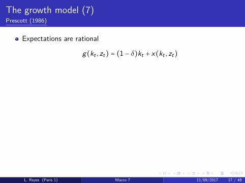
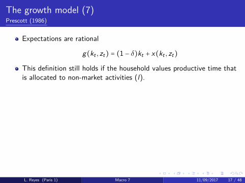
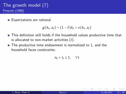
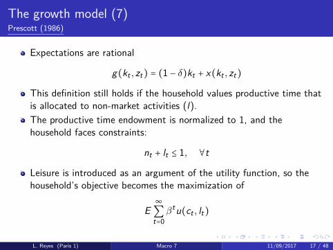
The growth model (7)Prescott (1986)
Expectations are rational
g(kt , zt) = (1 − δ)kt + x(kt , zt)
This definition still holds if the household values productive time thatis allocated to non-market activities (l).The productive time endowment is normalized to 1, and thehousehold faces constraints:
nt + lt ≤ 1, ∀t
Leisure is introduced as an argument of the utility function, so thehousehold’s objective becomes the maximization of
E∞∑t=0βtu(ct , lt)
L. Reyes (Paris 1) Macro 7 11/09/2017 17 / 48
The growth model (7)Prescott (1986)
Expectations are rational
g(kt , zt) = (1 − δ)kt + x(kt , zt)
This definition still holds if the household values productive time thatis allocated to non-market activities (l).
The productive time endowment is normalized to 1, and thehousehold faces constraints:
nt + lt ≤ 1, ∀t
Leisure is introduced as an argument of the utility function, so thehousehold’s objective becomes the maximization of
E∞∑t=0βtu(ct , lt)
L. Reyes (Paris 1) Macro 7 11/09/2017 17 / 48
The growth model (7)Prescott (1986)
Expectations are rational
g(kt , zt) = (1 − δ)kt + x(kt , zt)
This definition still holds if the household values productive time thatis allocated to non-market activities (l).The productive time endowment is normalized to 1, and thehousehold faces constraints:
nt + lt ≤ 1, ∀t
Leisure is introduced as an argument of the utility function, so thehousehold’s objective becomes the maximization of
E∞∑t=0βtu(ct , lt)
L. Reyes (Paris 1) Macro 7 11/09/2017 17 / 48
The growth model (7)Prescott (1986)
Expectations are rational
g(kt , zt) = (1 − δ)kt + x(kt , zt)
This definition still holds if the household values productive time thatis allocated to non-market activities (l).The productive time endowment is normalized to 1, and thehousehold faces constraints:
nt + lt ≤ 1, ∀t
Leisure is introduced as an argument of the utility function, so thehousehold’s objective becomes the maximization of
E∞∑t=0βtu(ct , lt)
L. Reyes (Paris 1) Macro 7 11/09/2017 17 / 48

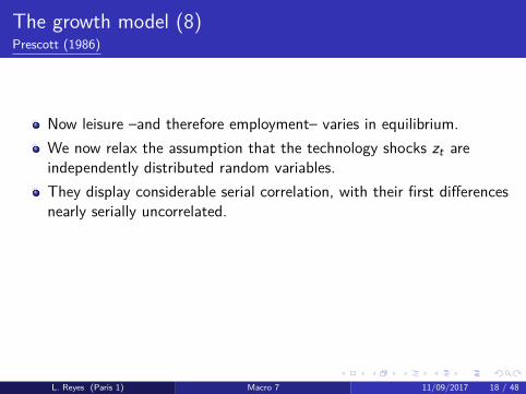
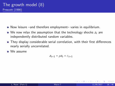
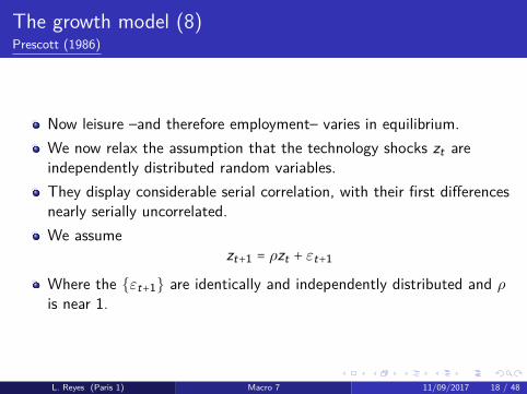
The growth model (8)Prescott (1986)
Now leisure –and therefore employment– varies in equilibrium.
We now relax the assumption that the technology shocks zt areindependently distributed random variables.They display considerable serial correlation, with their first differencesnearly serially uncorrelated.We assume
zt+1 = ρzt + εt+1
Where the {εt+1} are identically and independently distributed and ρis near 1.
L. Reyes (Paris 1) Macro 7 11/09/2017 18 / 48
The growth model (8)Prescott (1986)
Now leisure –and therefore employment– varies in equilibrium.We now relax the assumption that the technology shocks zt areindependently distributed random variables.
They display considerable serial correlation, with their first differencesnearly serially uncorrelated.We assume
zt+1 = ρzt + εt+1
Where the {εt+1} are identically and independently distributed and ρis near 1.
L. Reyes (Paris 1) Macro 7 11/09/2017 18 / 48
The growth model (8)Prescott (1986)
Now leisure –and therefore employment– varies in equilibrium.We now relax the assumption that the technology shocks zt areindependently distributed random variables.They display considerable serial correlation, with their first differencesnearly serially uncorrelated.
We assumezt+1 = ρzt + εt+1
Where the {εt+1} are identically and independently distributed and ρis near 1.
L. Reyes (Paris 1) Macro 7 11/09/2017 18 / 48
The growth model (8)Prescott (1986)
Now leisure –and therefore employment– varies in equilibrium.We now relax the assumption that the technology shocks zt areindependently distributed random variables.They display considerable serial correlation, with their first differencesnearly serially uncorrelated.We assume
zt+1 = ρzt + εt+1
Where the {εt+1} are identically and independently distributed and ρis near 1.
L. Reyes (Paris 1) Macro 7 11/09/2017 18 / 48
The growth model (8)Prescott (1986)
Now leisure –and therefore employment– varies in equilibrium.We now relax the assumption that the technology shocks zt areindependently distributed random variables.They display considerable serial correlation, with their first differencesnearly serially uncorrelated.We assume
zt+1 = ρzt + εt+1
Where the {εt+1} are identically and independently distributed and ρis near 1.
L. Reyes (Paris 1) Macro 7 11/09/2017 18 / 48

Outline
1 Real Business CyclesIntroductionBusiness cycle phenomena and growth modelUsing data to restrict the growth model, i.e. calibration
2 Dynamic Stochastic General Equilibrium modelsIntroductionThe linearized DSGE modelParameter estimates and model properties
L. Reyes (Paris 1) Macro 7 11/09/2017 19 / 48

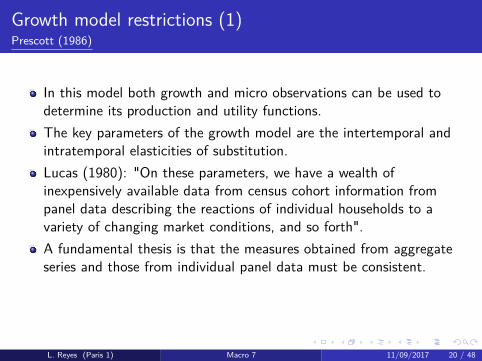
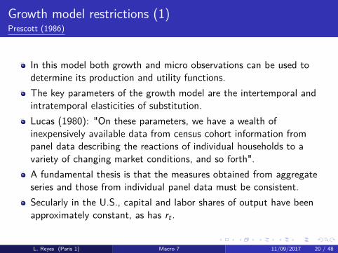
Growth model restrictions (1)Prescott (1986)
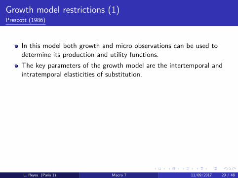
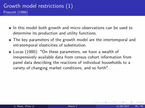
In this model both growth and micro observations can be used todetermine its production and utility functions.
The key parameters of the growth model are the intertemporal andintratemporal elasticities of substitution.Lucas (1980): "On these parameters, we have a wealth ofinexpensively available data from census cohort information frompanel data describing the reactions of individual households to avariety of changing market conditions, and so forth".A fundamental thesis is that the measures obtained from aggregateseries and those from individual panel data must be consistent.Secularly in the U.S., capital and labor shares of output have beenapproximately constant, as has rt .
L. Reyes (Paris 1) Macro 7 11/09/2017 20 / 48
Growth model restrictions (1)Prescott (1986)
In this model both growth and micro observations can be used todetermine its production and utility functions.The key parameters of the growth model are the intertemporal andintratemporal elasticities of substitution.
Lucas (1980): "On these parameters, we have a wealth ofinexpensively available data from census cohort information frompanel data describing the reactions of individual households to avariety of changing market conditions, and so forth".A fundamental thesis is that the measures obtained from aggregateseries and those from individual panel data must be consistent.Secularly in the U.S., capital and labor shares of output have beenapproximately constant, as has rt .
L. Reyes (Paris 1) Macro 7 11/09/2017 20 / 48
Growth model restrictions (1)Prescott (1986)
In this model both growth and micro observations can be used todetermine its production and utility functions.The key parameters of the growth model are the intertemporal andintratemporal elasticities of substitution.Lucas (1980): "On these parameters, we have a wealth ofinexpensively available data from census cohort information frompanel data describing the reactions of individual households to avariety of changing market conditions, and so forth".
A fundamental thesis is that the measures obtained from aggregateseries and those from individual panel data must be consistent.Secularly in the U.S., capital and labor shares of output have beenapproximately constant, as has rt .
L. Reyes (Paris 1) Macro 7 11/09/2017 20 / 48
Growth model restrictions (1)Prescott (1986)
In this model both growth and micro observations can be used todetermine its production and utility functions.The key parameters of the growth model are the intertemporal andintratemporal elasticities of substitution.Lucas (1980): "On these parameters, we have a wealth ofinexpensively available data from census cohort information frompanel data describing the reactions of individual households to avariety of changing market conditions, and so forth".A fundamental thesis is that the measures obtained from aggregateseries and those from individual panel data must be consistent.
Secularly in the U.S., capital and labor shares of output have beenapproximately constant, as has rt .
L. Reyes (Paris 1) Macro 7 11/09/2017 20 / 48
Growth model restrictions (1)Prescott (1986)
In this model both growth and micro observations can be used todetermine its production and utility functions.The key parameters of the growth model are the intertemporal andintratemporal elasticities of substitution.Lucas (1980): "On these parameters, we have a wealth ofinexpensively available data from census cohort information frompanel data describing the reactions of individual households to avariety of changing market conditions, and so forth".A fundamental thesis is that the measures obtained from aggregateseries and those from individual panel data must be consistent.Secularly in the U.S., capital and labor shares of output have beenapproximately constant, as has rt .
L. Reyes (Paris 1) Macro 7 11/09/2017 20 / 48
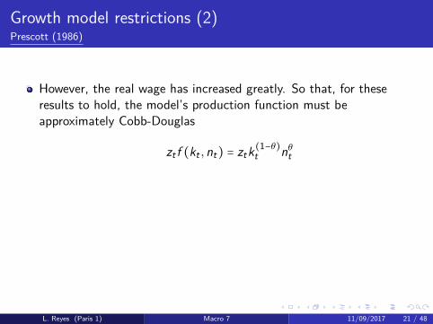
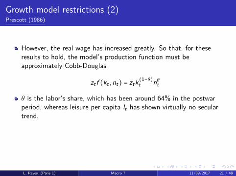
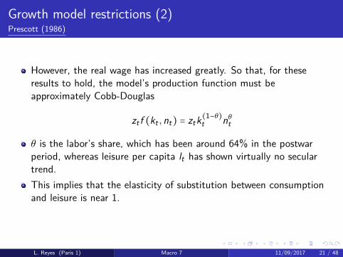
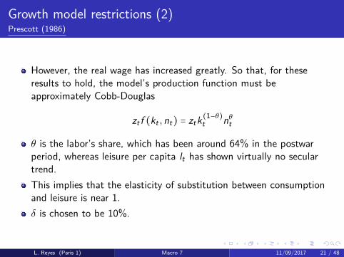
Growth model restrictions (2)Prescott (1986)
However, the real wage has increased greatly. So that, for theseresults to hold, the model’s production function must beapproximately Cobb-Douglas
zt f (kt ,nt) = ztk(1−θ)t nθt
θ is the labor’s share, which has been around 64% in the postwarperiod, whereas leisure per capita lt has shown virtually no seculartrend.This implies that the elasticity of substitution between consumptionand leisure is near 1.δ is chosen to be 10%.
L. Reyes (Paris 1) Macro 7 11/09/2017 21 / 48
Growth model restrictions (2)Prescott (1986)
However, the real wage has increased greatly. So that, for theseresults to hold, the model’s production function must beapproximately Cobb-Douglas
zt f (kt ,nt) = ztk(1−θ)t nθt
θ is the labor’s share, which has been around 64% in the postwarperiod, whereas leisure per capita lt has shown virtually no seculartrend.
This implies that the elasticity of substitution between consumptionand leisure is near 1.δ is chosen to be 10%.
L. Reyes (Paris 1) Macro 7 11/09/2017 21 / 48
Growth model restrictions (2)Prescott (1986)
However, the real wage has increased greatly. So that, for theseresults to hold, the model’s production function must beapproximately Cobb-Douglas
zt f (kt ,nt) = ztk(1−θ)t nθt
θ is the labor’s share, which has been around 64% in the postwarperiod, whereas leisure per capita lt has shown virtually no seculartrend.This implies that the elasticity of substitution between consumptionand leisure is near 1.
δ is chosen to be 10%.
L. Reyes (Paris 1) Macro 7 11/09/2017 21 / 48
Growth model restrictions (2)Prescott (1986)
However, the real wage has increased greatly. So that, for theseresults to hold, the model’s production function must beapproximately Cobb-Douglas
zt f (kt ,nt) = ztk(1−θ)t nθt
θ is the labor’s share, which has been around 64% in the postwarperiod, whereas leisure per capita lt has shown virtually no seculartrend.This implies that the elasticity of substitution between consumptionand leisure is near 1.δ is chosen to be 10%.
L. Reyes (Paris 1) Macro 7 11/09/2017 21 / 48

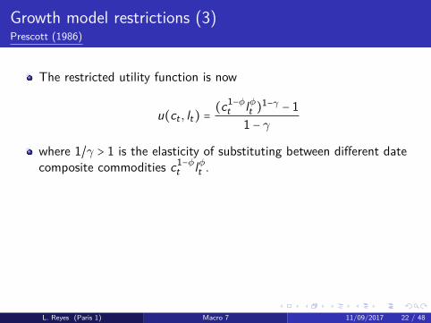
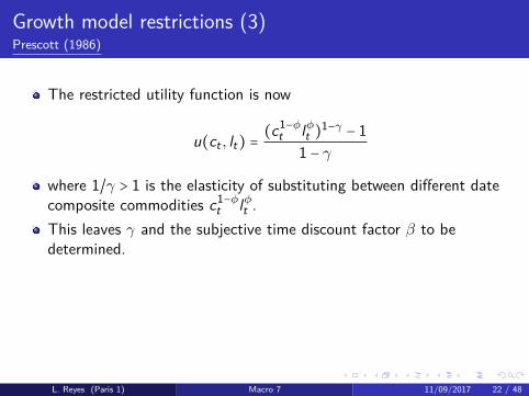
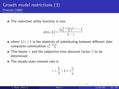
Growth model restrictions (3)Prescott (1986)
The restricted utility function is now
u(ct , lt) =(c1−φ
t lφt )1−γ − 11 − γ
where 1/γ > 1 is the elasticity of substituting between different datecomposite commodities c1−φ
t lφt .This leaves γ and the subjective time discount factor β to bedetermined.The steady-state interest rate is
i = 1β− 1 + γ c
c
L. Reyes (Paris 1) Macro 7 11/09/2017 22 / 48
Growth model restrictions (3)Prescott (1986)
The restricted utility function is now
u(ct , lt) =(c1−φ
t lφt )1−γ − 11 − γ
where 1/γ > 1 is the elasticity of substituting between different datecomposite commodities c1−φ
t lφt .
This leaves γ and the subjective time discount factor β to bedetermined.The steady-state interest rate is
i = 1β− 1 + γ c
c
L. Reyes (Paris 1) Macro 7 11/09/2017 22 / 48
Growth model restrictions (3)Prescott (1986)
The restricted utility function is now
u(ct , lt) =(c1−φ
t lφt )1−γ − 11 − γ
where 1/γ > 1 is the elasticity of substituting between different datecomposite commodities c1−φ
t lφt .This leaves γ and the subjective time discount factor β to bedetermined.
The steady-state interest rate is
i = 1β− 1 + γ c
c
L. Reyes (Paris 1) Macro 7 11/09/2017 22 / 48
Growth model restrictions (3)Prescott (1986)
The restricted utility function is now
u(ct , lt) =(c1−φ
t lφt )1−γ − 11 − γ
where 1/γ > 1 is the elasticity of substituting between different datecomposite commodities c1−φ
t lφt .This leaves γ and the subjective time discount factor β to bedetermined.The steady-state interest rate is
i = 1β− 1 + γ c
c
L. Reyes (Paris 1) Macro 7 11/09/2017 22 / 48
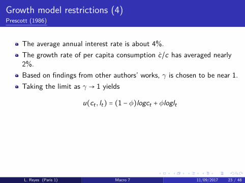
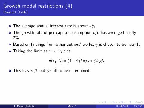
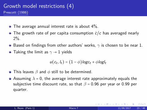
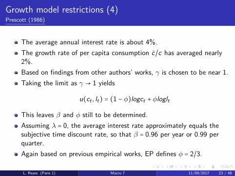
Growth model restrictions (4)Prescott (1986)
The average annual interest rate is about 4%.
The growth rate of per capita consumption c/c has averaged nearly2%.Based on findings from other authors’ works, γ is chosen to be near 1.Taking the limit as γ → 1 yields
u(ct , lt) = (1 − φ)logct + φloglt
This leaves β and φ still to be determined.Assuming λ = 0, the average interest rate approximately equals thesubjective time discount rate, so that β = 0.96 per year or 0.99 perquarter.Again based on previous empirical works, EP defines φ = 2/3.
L. Reyes (Paris 1) Macro 7 11/09/2017 23 / 48
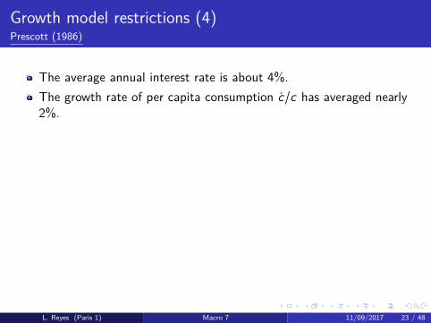
Growth model restrictions (4)Prescott (1986)
The average annual interest rate is about 4%.The growth rate of per capita consumption c/c has averaged nearly2%.
Based on findings from other authors’ works, γ is chosen to be near 1.Taking the limit as γ → 1 yields
u(ct , lt) = (1 − φ)logct + φloglt
This leaves β and φ still to be determined.Assuming λ = 0, the average interest rate approximately equals thesubjective time discount rate, so that β = 0.96 per year or 0.99 perquarter.Again based on previous empirical works, EP defines φ = 2/3.
L. Reyes (Paris 1) Macro 7 11/09/2017 23 / 48
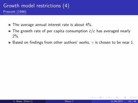
Growth model restrictions (4)Prescott (1986)
The average annual interest rate is about 4%.The growth rate of per capita consumption c/c has averaged nearly2%.Based on findings from other authors’ works, γ is chosen to be near 1.
Taking the limit as γ → 1 yields
u(ct , lt) = (1 − φ)logct + φloglt
This leaves β and φ still to be determined.Assuming λ = 0, the average interest rate approximately equals thesubjective time discount rate, so that β = 0.96 per year or 0.99 perquarter.Again based on previous empirical works, EP defines φ = 2/3.
L. Reyes (Paris 1) Macro 7 11/09/2017 23 / 48
Growth model restrictions (4)Prescott (1986)
The average annual interest rate is about 4%.The growth rate of per capita consumption c/c has averaged nearly2%.Based on findings from other authors’ works, γ is chosen to be near 1.Taking the limit as γ → 1 yields
u(ct , lt) = (1 − φ)logct + φloglt
This leaves β and φ still to be determined.
Assuming λ = 0, the average interest rate approximately equals thesubjective time discount rate, so that β = 0.96 per year or 0.99 perquarter.Again based on previous empirical works, EP defines φ = 2/3.
L. Reyes (Paris 1) Macro 7 11/09/2017 23 / 48
Growth model restrictions (4)Prescott (1986)
The average annual interest rate is about 4%.The growth rate of per capita consumption c/c has averaged nearly2%.Based on findings from other authors’ works, γ is chosen to be near 1.Taking the limit as γ → 1 yields
u(ct , lt) = (1 − φ)logct + φloglt
This leaves β and φ still to be determined.Assuming λ = 0, the average interest rate approximately equals thesubjective time discount rate, so that β = 0.96 per year or 0.99 perquarter.
Again based on previous empirical works, EP defines φ = 2/3.
L. Reyes (Paris 1) Macro 7 11/09/2017 23 / 48
Growth model restrictions (4)Prescott (1986)
The average annual interest rate is about 4%.The growth rate of per capita consumption c/c has averaged nearly2%.Based on findings from other authors’ works, γ is chosen to be near 1.Taking the limit as γ → 1 yields
u(ct , lt) = (1 − φ)logct + φloglt
This leaves β and φ still to be determined.Assuming λ = 0, the average interest rate approximately equals thesubjective time discount rate, so that β = 0.96 per year or 0.99 perquarter.Again based on previous empirical works, EP defines φ = 2/3.
L. Reyes (Paris 1) Macro 7 11/09/2017 23 / 48
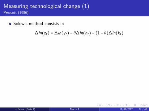
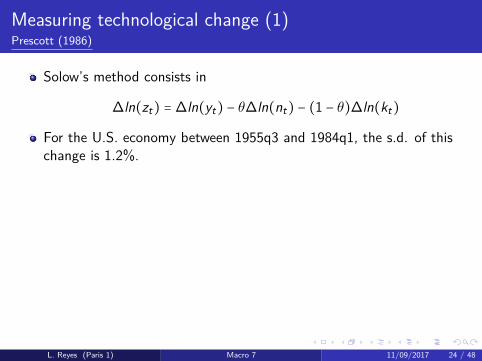
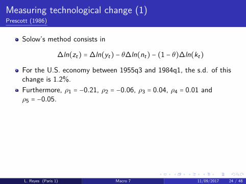
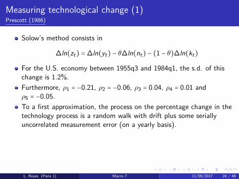
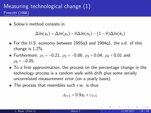
Measuring technological change (1)Prescott (1986)
Solow’s method consists in
∆ln(zt) = ∆ln(yt) − θ∆ln(nt) − (1 − θ)∆ln(kt)
For the U.S. economy between 1955q3 and 1984q1, the s.d. of thischange is 1.2%.Furthermore, ρ1 = −0.21, ρ2 = −0.06, ρ3 = 0.04, ρ4 = 0.01 andρ5 = −0.05.To a first approximation, the process on the percentage change in thetechnology process is a random walk with drift plus some seriallyuncorrelated measurement error (on a yearly basis).The process that resembles such r.w. is thus
zt+1 = 0.9zt + εt+1
L. Reyes (Paris 1) Macro 7 11/09/2017 24 / 48
Measuring technological change (1)Prescott (1986)
Solow’s method consists in
∆ln(zt) = ∆ln(yt) − θ∆ln(nt) − (1 − θ)∆ln(kt)
For the U.S. economy between 1955q3 and 1984q1, the s.d. of thischange is 1.2%.
Furthermore, ρ1 = −0.21, ρ2 = −0.06, ρ3 = 0.04, ρ4 = 0.01 andρ5 = −0.05.To a first approximation, the process on the percentage change in thetechnology process is a random walk with drift plus some seriallyuncorrelated measurement error (on a yearly basis).The process that resembles such r.w. is thus
zt+1 = 0.9zt + εt+1
L. Reyes (Paris 1) Macro 7 11/09/2017 24 / 48
Measuring technological change (1)Prescott (1986)
Solow’s method consists in
∆ln(zt) = ∆ln(yt) − θ∆ln(nt) − (1 − θ)∆ln(kt)
For the U.S. economy between 1955q3 and 1984q1, the s.d. of thischange is 1.2%.Furthermore, ρ1 = −0.21, ρ2 = −0.06, ρ3 = 0.04, ρ4 = 0.01 andρ5 = −0.05.
To a first approximation, the process on the percentage change in thetechnology process is a random walk with drift plus some seriallyuncorrelated measurement error (on a yearly basis).The process that resembles such r.w. is thus
zt+1 = 0.9zt + εt+1
L. Reyes (Paris 1) Macro 7 11/09/2017 24 / 48
Measuring technological change (1)Prescott (1986)
Solow’s method consists in
∆ln(zt) = ∆ln(yt) − θ∆ln(nt) − (1 − θ)∆ln(kt)
For the U.S. economy between 1955q3 and 1984q1, the s.d. of thischange is 1.2%.Furthermore, ρ1 = −0.21, ρ2 = −0.06, ρ3 = 0.04, ρ4 = 0.01 andρ5 = −0.05.To a first approximation, the process on the percentage change in thetechnology process is a random walk with drift plus some seriallyuncorrelated measurement error (on a yearly basis).
The process that resembles such r.w. is thus
zt+1 = 0.9zt + εt+1
L. Reyes (Paris 1) Macro 7 11/09/2017 24 / 48
Measuring technological change (1)Prescott (1986)
Solow’s method consists in
∆ln(zt) = ∆ln(yt) − θ∆ln(nt) − (1 − θ)∆ln(kt)
For the U.S. economy between 1955q3 and 1984q1, the s.d. of thischange is 1.2%.Furthermore, ρ1 = −0.21, ρ2 = −0.06, ρ3 = 0.04, ρ4 = 0.01 andρ5 = −0.05.To a first approximation, the process on the percentage change in thetechnology process is a random walk with drift plus some seriallyuncorrelated measurement error (on a yearly basis).The process that resembles such r.w. is thus
zt+1 = 0.9zt + εt+1
L. Reyes (Paris 1) Macro 7 11/09/2017 24 / 48

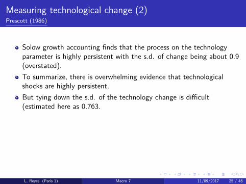
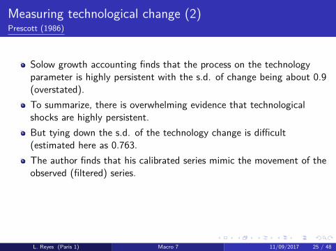
Measuring technological change (2)Prescott (1986)
Solow growth accounting finds that the process on the technologyparameter is highly persistent with the s.d. of change being about 0.9(overstated).
To summarize, there is overwhelming evidence that technologicalshocks are highly persistent.But tying down the s.d. of the technology change is difficult(estimated here as 0.763.The author finds that his calibrated series mimic the movement of theobserved (filtered) series.The story goes on and on, but these are the main elements of theRBC model that makes up the basis of the DSGE model seen next.
But before that, the summary and policy implications.
L. Reyes (Paris 1) Macro 7 11/09/2017 25 / 48

Measuring technological change (2)Prescott (1986)
Solow growth accounting finds that the process on the technologyparameter is highly persistent with the s.d. of change being about 0.9(overstated).To summarize, there is overwhelming evidence that technologicalshocks are highly persistent.
But tying down the s.d. of the technology change is difficult(estimated here as 0.763.The author finds that his calibrated series mimic the movement of theobserved (filtered) series.The story goes on and on, but these are the main elements of theRBC model that makes up the basis of the DSGE model seen next.
But before that, the summary and policy implications.
L. Reyes (Paris 1) Macro 7 11/09/2017 25 / 48
Measuring technological change (2)Prescott (1986)
Solow growth accounting finds that the process on the technologyparameter is highly persistent with the s.d. of change being about 0.9(overstated).To summarize, there is overwhelming evidence that technologicalshocks are highly persistent.But tying down the s.d. of the technology change is difficult(estimated here as 0.763.
The author finds that his calibrated series mimic the movement of theobserved (filtered) series.The story goes on and on, but these are the main elements of theRBC model that makes up the basis of the DSGE model seen next.
But before that, the summary and policy implications.
L. Reyes (Paris 1) Macro 7 11/09/2017 25 / 48
Measuring technological change (2)Prescott (1986)
Solow growth accounting finds that the process on the technologyparameter is highly persistent with the s.d. of change being about 0.9(overstated).To summarize, there is overwhelming evidence that technologicalshocks are highly persistent.But tying down the s.d. of the technology change is difficult(estimated here as 0.763.The author finds that his calibrated series mimic the movement of theobserved (filtered) series.
The story goes on and on, but these are the main elements of theRBC model that makes up the basis of the DSGE model seen next.
But before that, the summary and policy implications.
L. Reyes (Paris 1) Macro 7 11/09/2017 25 / 48

Measuring technological change (2)Prescott (1986)
Solow growth accounting finds that the process on the technologyparameter is highly persistent with the s.d. of change being about 0.9(overstated).To summarize, there is overwhelming evidence that technologicalshocks are highly persistent.But tying down the s.d. of the technology change is difficult(estimated here as 0.763.The author finds that his calibrated series mimic the movement of theobserved (filtered) series.The story goes on and on, but these are the main elements of theRBC model that makes up the basis of the DSGE model seen next.
But before that, the summary and policy implications.
L. Reyes (Paris 1) Macro 7 11/09/2017 25 / 48

Measuring technological change (2)Prescott (1986)
Solow growth accounting finds that the process on the technologyparameter is highly persistent with the s.d. of change being about 0.9(overstated).To summarize, there is overwhelming evidence that technologicalshocks are highly persistent.But tying down the s.d. of the technology change is difficult(estimated here as 0.763.The author finds that his calibrated series mimic the movement of theobserved (filtered) series.The story goes on and on, but these are the main elements of theRBC model that makes up the basis of the DSGE model seen next.But before that, the summary and policy implications.
L. Reyes (Paris 1) Macro 7 11/09/2017 25 / 48
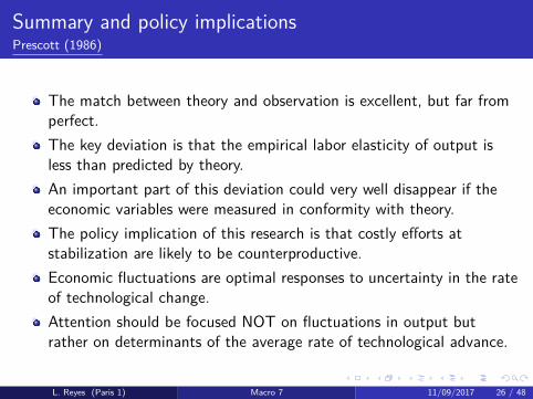
Summary and policy implicationsPrescott (1986)
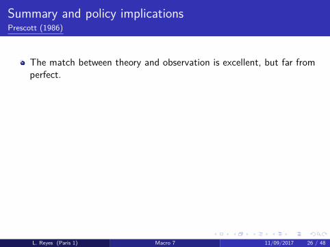
The match between theory and observation is excellent, but far fromperfect.
The key deviation is that the empirical labor elasticity of output isless than predicted by theory.An important part of this deviation could very well disappear if theeconomic variables were measured in conformity with theory.The policy implication of this research is that costly efforts atstabilization are likely to be counterproductive.Economic fluctuations are optimal responses to uncertainty in the rateof technological change.Attention should be focused NOT on fluctuations in output butrather on determinants of the average rate of technological advance.
L. Reyes (Paris 1) Macro 7 11/09/2017 26 / 48
Summary and policy implicationsPrescott (1986)
The match between theory and observation is excellent, but far fromperfect.The key deviation is that the empirical labor elasticity of output isless than predicted by theory.
An important part of this deviation could very well disappear if theeconomic variables were measured in conformity with theory.The policy implication of this research is that costly efforts atstabilization are likely to be counterproductive.Economic fluctuations are optimal responses to uncertainty in the rateof technological change.Attention should be focused NOT on fluctuations in output butrather on determinants of the average rate of technological advance.
L. Reyes (Paris 1) Macro 7 11/09/2017 26 / 48
Summary and policy implicationsPrescott (1986)
The match between theory and observation is excellent, but far fromperfect.The key deviation is that the empirical labor elasticity of output isless than predicted by theory.An important part of this deviation could very well disappear if theeconomic variables were measured in conformity with theory.
The policy implication of this research is that costly efforts atstabilization are likely to be counterproductive.Economic fluctuations are optimal responses to uncertainty in the rateof technological change.Attention should be focused NOT on fluctuations in output butrather on determinants of the average rate of technological advance.
L. Reyes (Paris 1) Macro 7 11/09/2017 26 / 48
Summary and policy implicationsPrescott (1986)
The match between theory and observation is excellent, but far fromperfect.The key deviation is that the empirical labor elasticity of output isless than predicted by theory.An important part of this deviation could very well disappear if theeconomic variables were measured in conformity with theory.The policy implication of this research is that costly efforts atstabilization are likely to be counterproductive.
Economic fluctuations are optimal responses to uncertainty in the rateof technological change.Attention should be focused NOT on fluctuations in output butrather on determinants of the average rate of technological advance.
L. Reyes (Paris 1) Macro 7 11/09/2017 26 / 48
Summary and policy implicationsPrescott (1986)
The match between theory and observation is excellent, but far fromperfect.The key deviation is that the empirical labor elasticity of output isless than predicted by theory.An important part of this deviation could very well disappear if theeconomic variables were measured in conformity with theory.The policy implication of this research is that costly efforts atstabilization are likely to be counterproductive.Economic fluctuations are optimal responses to uncertainty in the rateof technological change.
Attention should be focused NOT on fluctuations in output butrather on determinants of the average rate of technological advance.
L. Reyes (Paris 1) Macro 7 11/09/2017 26 / 48
Summary and policy implicationsPrescott (1986)
The match between theory and observation is excellent, but far fromperfect.The key deviation is that the empirical labor elasticity of output isless than predicted by theory.An important part of this deviation could very well disappear if theeconomic variables were measured in conformity with theory.The policy implication of this research is that costly efforts atstabilization are likely to be counterproductive.Economic fluctuations are optimal responses to uncertainty in the rateof technological change.Attention should be focused NOT on fluctuations in output butrather on determinants of the average rate of technological advance.
L. Reyes (Paris 1) Macro 7 11/09/2017 26 / 48

Outline
1 Real Business CyclesIntroductionBusiness cycle phenomena and growth modelUsing data to restrict the growth model, i.e. calibration
2 Dynamic Stochastic General Equilibrium modelsIntroductionThe linearized DSGE modelParameter estimates and model properties
L. Reyes (Paris 1) Macro 7 11/09/2017 27 / 48

Outline
1 Real Business CyclesIntroductionBusiness cycle phenomena and growth modelUsing data to restrict the growth model, i.e. calibration
2 Dynamic Stochastic General Equilibrium modelsIntroductionThe linearized DSGE modelParameter estimates and model properties
L. Reyes (Paris 1) Macro 7 11/09/2017 28 / 48
Introduction (1)
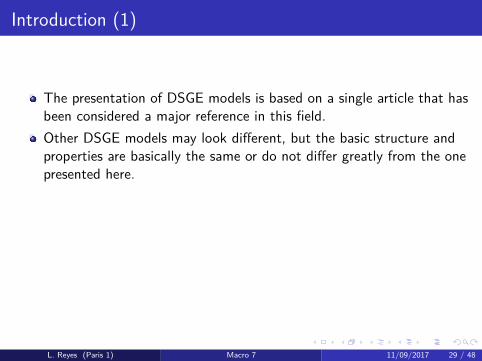
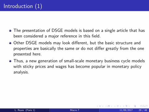
The presentation of DSGE models is based on a single article that hasbeen considered a major reference in this field.
Other DSGE models may look different, but the basic structure andproperties are basically the same or do not differ greatly from the onepresented here.Thus, a new generation of small-scale monetary business cycle modelswith sticky prices and wages has become popular in monetary policyanalysis.These models are called New Keynesian or New NeoclassicalSynthesis (NNS).
L. Reyes (Paris 1) Macro 7 11/09/2017 29 / 48
Introduction (1)
The presentation of DSGE models is based on a single article that hasbeen considered a major reference in this field.Other DSGE models may look different, but the basic structure andproperties are basically the same or do not differ greatly from the onepresented here.
Thus, a new generation of small-scale monetary business cycle modelswith sticky prices and wages has become popular in monetary policyanalysis.These models are called New Keynesian or New NeoclassicalSynthesis (NNS).
L. Reyes (Paris 1) Macro 7 11/09/2017 29 / 48
Introduction (1)
The presentation of DSGE models is based on a single article that hasbeen considered a major reference in this field.Other DSGE models may look different, but the basic structure andproperties are basically the same or do not differ greatly from the onepresented here.Thus, a new generation of small-scale monetary business cycle modelswith sticky prices and wages has become popular in monetary policyanalysis.
These models are called New Keynesian or New NeoclassicalSynthesis (NNS).
L. Reyes (Paris 1) Macro 7 11/09/2017 29 / 48
Introduction (1)
The presentation of DSGE models is based on a single article that hasbeen considered a major reference in this field.Other DSGE models may look different, but the basic structure andproperties are basically the same or do not differ greatly from the onepresented here.Thus, a new generation of small-scale monetary business cycle modelswith sticky prices and wages has become popular in monetary policyanalysis.These models are called New Keynesian or New NeoclassicalSynthesis (NNS).
L. Reyes (Paris 1) Macro 7 11/09/2017 29 / 48

Introduction (2)Smets and Wouters, 2007
The objectives of the authors are threefold
1 As the NNS models have become the standard workhorse for monetarypolicy analysis, it is important to verify whether they can explain themain features of the U.S. macro data.
2 The introduction of a large number of fictions raises the questionwhether each of these are really necessary to describe the 7 data series.
3 They use the estimated NNS model to address a number of key issues.These issues are:
(1) the main driving forces of output developmentsin the U.S., (2) prove that productivity shocks have a significantshort-run negative impact on hours worked, (3) inflationdevelopments are mostly driven by the price mark-up shocks in theshort run and the wage mark-up in the long run.
L. Reyes (Paris 1) Macro 7 11/09/2017 30 / 48
Introduction (2)Smets and Wouters, 2007
The objectives of the authors are threefold1 As the NNS models have become the standard workhorse for monetary
policy analysis, it is important to verify whether they can explain themain features of the U.S. macro data.
2 The introduction of a large number of fictions raises the questionwhether each of these are really necessary to describe the 7 data series.
3 They use the estimated NNS model to address a number of key issues.These issues are:
(1) the main driving forces of output developmentsin the U.S., (2) prove that productivity shocks have a significantshort-run negative impact on hours worked, (3) inflationdevelopments are mostly driven by the price mark-up shocks in theshort run and the wage mark-up in the long run.
L. Reyes (Paris 1) Macro 7 11/09/2017 30 / 48
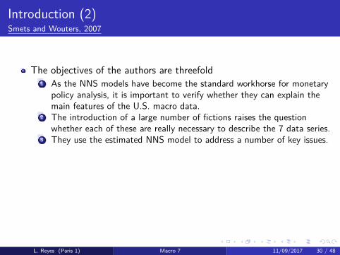
Introduction (2)Smets and Wouters, 2007
The objectives of the authors are threefold1 As the NNS models have become the standard workhorse for monetary
policy analysis, it is important to verify whether they can explain themain features of the U.S. macro data.
2 The introduction of a large number of fictions raises the questionwhether each of these are really necessary to describe the 7 data series.
3 They use the estimated NNS model to address a number of key issues.
These issues are:
(1) the main driving forces of output developmentsin the U.S., (2) prove that productivity shocks have a significantshort-run negative impact on hours worked, (3) inflationdevelopments are mostly driven by the price mark-up shocks in theshort run and the wage mark-up in the long run.
L. Reyes (Paris 1) Macro 7 11/09/2017 30 / 48
Introduction (2)Smets and Wouters, 2007
The objectives of the authors are threefold1 As the NNS models have become the standard workhorse for monetary
policy analysis, it is important to verify whether they can explain themain features of the U.S. macro data.
2 The introduction of a large number of fictions raises the questionwhether each of these are really necessary to describe the 7 data series.
3 They use the estimated NNS model to address a number of key issues.These issues are:
(1) the main driving forces of output developmentsin the U.S., (2) prove that productivity shocks have a significantshort-run negative impact on hours worked, (3) inflationdevelopments are mostly driven by the price mark-up shocks in theshort run and the wage mark-up in the long run.
L. Reyes (Paris 1) Macro 7 11/09/2017 30 / 48

Introduction (2)Smets and Wouters, 2007
The objectives of the authors are threefold1 As the NNS models have become the standard workhorse for monetary
policy analysis, it is important to verify whether they can explain themain features of the U.S. macro data.
2 The introduction of a large number of fictions raises the questionwhether each of these are really necessary to describe the 7 data series.
3 They use the estimated NNS model to address a number of key issues.These issues are:
(1) the main driving forces of output developmentsin the U.S., (2) prove that productivity shocks have a significantshort-run negative impact on hours worked, (3) inflationdevelopments are mostly driven by the price mark-up shocks in theshort run and the wage mark-up in the long run.
L. Reyes (Paris 1) Macro 7 11/09/2017 30 / 48
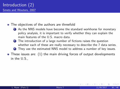
Introduction (2)Smets and Wouters, 2007
The objectives of the authors are threefold1 As the NNS models have become the standard workhorse for monetary
policy analysis, it is important to verify whether they can explain themain features of the U.S. macro data.
2 The introduction of a large number of fictions raises the questionwhether each of these are really necessary to describe the 7 data series.
3 They use the estimated NNS model to address a number of key issues.These issues are: (1) the main driving forces of output developmentsin the U.S.,
(2) prove that productivity shocks have a significantshort-run negative impact on hours worked, (3) inflationdevelopments are mostly driven by the price mark-up shocks in theshort run and the wage mark-up in the long run.
L. Reyes (Paris 1) Macro 7 11/09/2017 30 / 48
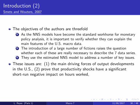
Introduction (2)Smets and Wouters, 2007
The objectives of the authors are threefold1 As the NNS models have become the standard workhorse for monetary
policy analysis, it is important to verify whether they can explain themain features of the U.S. macro data.
2 The introduction of a large number of fictions raises the questionwhether each of these are really necessary to describe the 7 data series.
3 They use the estimated NNS model to address a number of key issues.These issues are: (1) the main driving forces of output developmentsin the U.S., (2) prove that productivity shocks have a significantshort-run negative impact on hours worked,
(3) inflationdevelopments are mostly driven by the price mark-up shocks in theshort run and the wage mark-up in the long run.
L. Reyes (Paris 1) Macro 7 11/09/2017 30 / 48
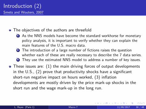
Introduction (2)Smets and Wouters, 2007
The objectives of the authors are threefold1 As the NNS models have become the standard workhorse for monetary
policy analysis, it is important to verify whether they can explain themain features of the U.S. macro data.
2 The introduction of a large number of fictions raises the questionwhether each of these are really necessary to describe the 7 data series.
3 They use the estimated NNS model to address a number of key issues.These issues are: (1) the main driving forces of output developmentsin the U.S., (2) prove that productivity shocks have a significantshort-run negative impact on hours worked, (3) inflationdevelopments are mostly driven by the price mark-up shocks in theshort run and the wage mark-up in the long run.
L. Reyes (Paris 1) Macro 7 11/09/2017 30 / 48

Outline
1 Real Business CyclesIntroductionBusiness cycle phenomena and growth modelUsing data to restrict the growth model, i.e. calibration
2 Dynamic Stochastic General Equilibrium modelsIntroductionThe linearized DSGE modelParameter estimates and model properties
L. Reyes (Paris 1) Macro 7 11/09/2017 31 / 48

The linearized DSGE model (1)Smets and Wouters, 2007
This is an extension that is consistent with a balanced steady stategrowth path driven by deterministic labor-augmenting technologicalprogress.
Households maximize a non-separable utility function with twoarguments (goods and labor effort) over an infinite horizon.Consumption appears in the utility function relative to a time-varyingexternal habit variable.Labor is differentiated by a union, so that there is some monopolypower over wages.Households rent capital services to firms and decide how much capitalto accumulate given the capital adjustment costs they face.
L. Reyes (Paris 1) Macro 7 11/09/2017 32 / 48
The linearized DSGE model (1)Smets and Wouters, 2007
This is an extension that is consistent with a balanced steady stategrowth path driven by deterministic labor-augmenting technologicalprogress.Households maximize a non-separable utility function with twoarguments (goods and labor effort) over an infinite horizon.
Consumption appears in the utility function relative to a time-varyingexternal habit variable.Labor is differentiated by a union, so that there is some monopolypower over wages.Households rent capital services to firms and decide how much capitalto accumulate given the capital adjustment costs they face.
L. Reyes (Paris 1) Macro 7 11/09/2017 32 / 48
The linearized DSGE model (1)Smets and Wouters, 2007
This is an extension that is consistent with a balanced steady stategrowth path driven by deterministic labor-augmenting technologicalprogress.Households maximize a non-separable utility function with twoarguments (goods and labor effort) over an infinite horizon.Consumption appears in the utility function relative to a time-varyingexternal habit variable.
Labor is differentiated by a union, so that there is some monopolypower over wages.Households rent capital services to firms and decide how much capitalto accumulate given the capital adjustment costs they face.
L. Reyes (Paris 1) Macro 7 11/09/2017 32 / 48

The linearized DSGE model (1)Smets and Wouters, 2007
This is an extension that is consistent with a balanced steady stategrowth path driven by deterministic labor-augmenting technologicalprogress.Households maximize a non-separable utility function with twoarguments (goods and labor effort) over an infinite horizon.Consumption appears in the utility function relative to a time-varyingexternal habit variable.Labor is differentiated by a union, so that there is some monopolypower over wages.
Households rent capital services to firms and decide how much capitalto accumulate given the capital adjustment costs they face.
L. Reyes (Paris 1) Macro 7 11/09/2017 32 / 48

The linearized DSGE model (1)Smets and Wouters, 2007
This is an extension that is consistent with a balanced steady stategrowth path driven by deterministic labor-augmenting technologicalprogress.Households maximize a non-separable utility function with twoarguments (goods and labor effort) over an infinite horizon.Consumption appears in the utility function relative to a time-varyingexternal habit variable.Labor is differentiated by a union, so that there is some monopolypower over wages.Households rent capital services to firms and decide how much capitalto accumulate given the capital adjustment costs they face.
L. Reyes (Paris 1) Macro 7 11/09/2017 32 / 48
The linearized DSGE model (2)Smets and Wouters, 2007
Prices are set in function of current and expected marginal costs, butare also determined by the past inflation rate.
SW introduce a time-varying demand elasticity which depends on therelative price (more reasonable degree of price and wage stickiness).The aggregate resource constraint is:
yt = cyct + iy it + zyzt + εgt
Output (yt) is absorbed by consumption (ct), investment (it),capital-utilization costs that are a function of the capital utilizationrate (zt), and exogenous spending (εg
t ).cy is the ss share of consumption in output (1− gy − iy ), where gy andiy are respectively the ss exogenous spending-output andinvestment-output ratios.
L. Reyes (Paris 1) Macro 7 11/09/2017 33 / 48
The linearized DSGE model (2)Smets and Wouters, 2007
Prices are set in function of current and expected marginal costs, butare also determined by the past inflation rate.SW introduce a time-varying demand elasticity which depends on therelative price (more reasonable degree of price and wage stickiness).
The aggregate resource constraint is:
yt = cyct + iy it + zyzt + εgt
Output (yt) is absorbed by consumption (ct), investment (it),capital-utilization costs that are a function of the capital utilizationrate (zt), and exogenous spending (εg
t ).cy is the ss share of consumption in output (1− gy − iy ), where gy andiy are respectively the ss exogenous spending-output andinvestment-output ratios.
L. Reyes (Paris 1) Macro 7 11/09/2017 33 / 48
The linearized DSGE model (2)Smets and Wouters, 2007
Prices are set in function of current and expected marginal costs, butare also determined by the past inflation rate.SW introduce a time-varying demand elasticity which depends on therelative price (more reasonable degree of price and wage stickiness).The aggregate resource constraint is:
yt = cyct + iy it + zyzt + εgt
Output (yt) is absorbed by consumption (ct), investment (it),capital-utilization costs that are a function of the capital utilizationrate (zt), and exogenous spending (εg
t ).
cy is the ss share of consumption in output (1− gy − iy ), where gy andiy are respectively the ss exogenous spending-output andinvestment-output ratios.
L. Reyes (Paris 1) Macro 7 11/09/2017 33 / 48
The linearized DSGE model (2)Smets and Wouters, 2007
Prices are set in function of current and expected marginal costs, butare also determined by the past inflation rate.SW introduce a time-varying demand elasticity which depends on therelative price (more reasonable degree of price and wage stickiness).The aggregate resource constraint is:
yt = cyct + iy it + zyzt + εgt
Output (yt) is absorbed by consumption (ct), investment (it),capital-utilization costs that are a function of the capital utilizationrate (zt), and exogenous spending (εg
t ).cy is the ss share of consumption in output (1− gy − iy ), where gy andiy are respectively the ss exogenous spending-output andinvestment-output ratios.
L. Reyes (Paris 1) Macro 7 11/09/2017 33 / 48
The linearized DSGE model (3)Smets and Wouters, 2007
The ss investment-output ratio equals (γ − 1 + δ)ky , where γ is the ssgrowth rate, δ is the depreciation rate of capital and ky is the sscapital-output ratio.
zy = Rk∗ky where Rk∗ is the ss rental rate of capital.We assume that exogenous spending follows a AR(1) process withi.i.d. normal error term, and is affected by the productivity shock asfollows
εgt = ρgε
gt−1 + η
gt + ρgaη
at
In estimation, εgt also includes net exports, which may be affected by
domestic productivity developments.
L. Reyes (Paris 1) Macro 7 11/09/2017 34 / 48
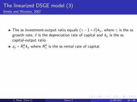
The linearized DSGE model (3)Smets and Wouters, 2007
The ss investment-output ratio equals (γ − 1 + δ)ky , where γ is the ssgrowth rate, δ is the depreciation rate of capital and ky is the sscapital-output ratio.zy = Rk∗ky where Rk∗ is the ss rental rate of capital.
We assume that exogenous spending follows a AR(1) process withi.i.d. normal error term, and is affected by the productivity shock asfollows
εgt = ρgε
gt−1 + η
gt + ρgaη
at
In estimation, εgt also includes net exports, which may be affected by
domestic productivity developments.
L. Reyes (Paris 1) Macro 7 11/09/2017 34 / 48
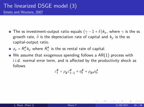
The linearized DSGE model (3)Smets and Wouters, 2007
The ss investment-output ratio equals (γ − 1 + δ)ky , where γ is the ssgrowth rate, δ is the depreciation rate of capital and ky is the sscapital-output ratio.zy = Rk∗ky where Rk∗ is the ss rental rate of capital.We assume that exogenous spending follows a AR(1) process withi.i.d. normal error term, and is affected by the productivity shock asfollows
εgt = ρgε
gt−1 + η
gt + ρgaη
at
In estimation, εgt also includes net exports, which may be affected by
domestic productivity developments.
L. Reyes (Paris 1) Macro 7 11/09/2017 34 / 48
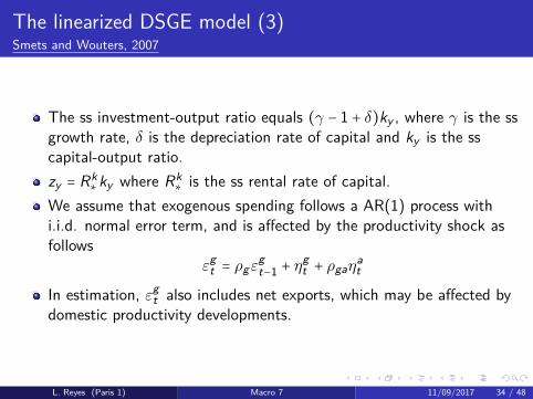
The linearized DSGE model (3)Smets and Wouters, 2007
The ss investment-output ratio equals (γ − 1 + δ)ky , where γ is the ssgrowth rate, δ is the depreciation rate of capital and ky is the sscapital-output ratio.zy = Rk∗ky where Rk∗ is the ss rental rate of capital.We assume that exogenous spending follows a AR(1) process withi.i.d. normal error term, and is affected by the productivity shock asfollows
εgt = ρgε
gt−1 + η
gt + ρgaη
at
In estimation, εgt also includes net exports, which may be affected by
domestic productivity developments.
L. Reyes (Paris 1) Macro 7 11/09/2017 34 / 48
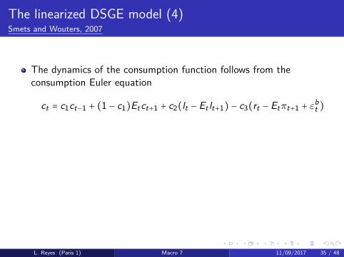
The linearized DSGE model (4)Smets and Wouters, 2007
The dynamics of the consumption function follows from theconsumption Euler equation
ct = c1ct−1 + (1 − c1)Etct+1 + c2(lt − Et lt+1) − c3(rt − Etπt+1 + εbt )
ct depends on a weighted average of past and expected futureconsumption, and on expected growth in hours worked, the ex-antereal interest rate and a disturbance term.The parameters c1, c2 and c3 are calibrated.If we assume that there is no external habit formation (λ = 0) and thelog utility in consumption (σc = 1), c1 = c2 = 0, and the purelyforward-looking consumption function is obtained.
L. Reyes (Paris 1) Macro 7 11/09/2017 35 / 48
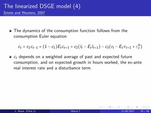
The linearized DSGE model (4)Smets and Wouters, 2007
The dynamics of the consumption function follows from theconsumption Euler equation
ct = c1ct−1 + (1 − c1)Etct+1 + c2(lt − Et lt+1) − c3(rt − Etπt+1 + εbt )
ct depends on a weighted average of past and expected futureconsumption, and on expected growth in hours worked, the ex-antereal interest rate and a disturbance term.
The parameters c1, c2 and c3 are calibrated.If we assume that there is no external habit formation (λ = 0) and thelog utility in consumption (σc = 1), c1 = c2 = 0, and the purelyforward-looking consumption function is obtained.
L. Reyes (Paris 1) Macro 7 11/09/2017 35 / 48
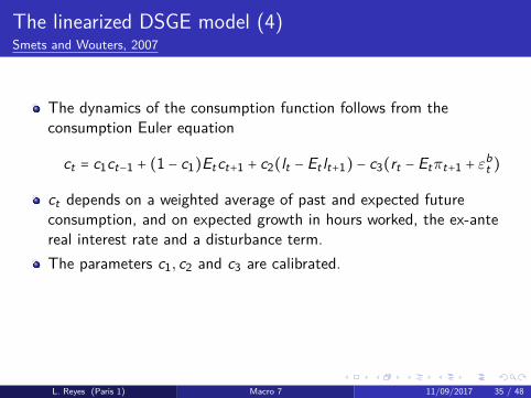
The linearized DSGE model (4)Smets and Wouters, 2007
The dynamics of the consumption function follows from theconsumption Euler equation
ct = c1ct−1 + (1 − c1)Etct+1 + c2(lt − Et lt+1) − c3(rt − Etπt+1 + εbt )
ct depends on a weighted average of past and expected futureconsumption, and on expected growth in hours worked, the ex-antereal interest rate and a disturbance term.The parameters c1, c2 and c3 are calibrated.
If we assume that there is no external habit formation (λ = 0) and thelog utility in consumption (σc = 1), c1 = c2 = 0, and the purelyforward-looking consumption function is obtained.
L. Reyes (Paris 1) Macro 7 11/09/2017 35 / 48
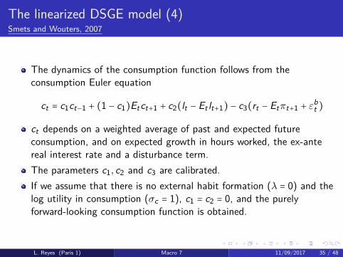
The linearized DSGE model (4)Smets and Wouters, 2007
The dynamics of the consumption function follows from theconsumption Euler equation
ct = c1ct−1 + (1 − c1)Etct+1 + c2(lt − Et lt+1) − c3(rt − Etπt+1 + εbt )
ct depends on a weighted average of past and expected futureconsumption, and on expected growth in hours worked, the ex-antereal interest rate and a disturbance term.The parameters c1, c2 and c3 are calibrated.If we assume that there is no external habit formation (λ = 0) and thelog utility in consumption (σc = 1), c1 = c2 = 0, and the purelyforward-looking consumption function is obtained.
L. Reyes (Paris 1) Macro 7 11/09/2017 35 / 48
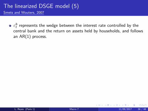
The linearized DSGE model (5)Smets and Wouters, 2007
εbt represents the wedge between the interest rate controlled by thecentral bank and the return on assets held by households, and followsan AR(1) process.
A positive shock to this wedge increases the required return on assetsheld by households.At the same time, it increases the cost of capital and reduces thevalue of capital and investment (net-worth shocks).The dynamics of investment comes from the investment Eulerequation
it = i1it−1 + (1 − i1)Et it+1 + i2qt + εit
A higher elasticity of the cost of adjusting capital reduces thesensitivity of investment (it) to the real value of existing capital stock(qt).
L. Reyes (Paris 1) Macro 7 11/09/2017 36 / 48
The linearized DSGE model (5)Smets and Wouters, 2007
εbt represents the wedge between the interest rate controlled by thecentral bank and the return on assets held by households, and followsan AR(1) process.A positive shock to this wedge increases the required return on assetsheld by households.
At the same time, it increases the cost of capital and reduces thevalue of capital and investment (net-worth shocks).The dynamics of investment comes from the investment Eulerequation
it = i1it−1 + (1 − i1)Et it+1 + i2qt + εit
A higher elasticity of the cost of adjusting capital reduces thesensitivity of investment (it) to the real value of existing capital stock(qt).
L. Reyes (Paris 1) Macro 7 11/09/2017 36 / 48
The linearized DSGE model (5)Smets and Wouters, 2007
εbt represents the wedge between the interest rate controlled by thecentral bank and the return on assets held by households, and followsan AR(1) process.A positive shock to this wedge increases the required return on assetsheld by households.At the same time, it increases the cost of capital and reduces thevalue of capital and investment (net-worth shocks).
The dynamics of investment comes from the investment Eulerequation
it = i1it−1 + (1 − i1)Et it+1 + i2qt + εit
A higher elasticity of the cost of adjusting capital reduces thesensitivity of investment (it) to the real value of existing capital stock(qt).
L. Reyes (Paris 1) Macro 7 11/09/2017 36 / 48
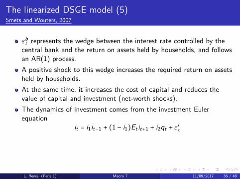
The linearized DSGE model (5)Smets and Wouters, 2007
εbt represents the wedge between the interest rate controlled by thecentral bank and the return on assets held by households, and followsan AR(1) process.A positive shock to this wedge increases the required return on assetsheld by households.At the same time, it increases the cost of capital and reduces thevalue of capital and investment (net-worth shocks).The dynamics of investment comes from the investment Eulerequation
it = i1it−1 + (1 − i1)Et it+1 + i2qt + εit
A higher elasticity of the cost of adjusting capital reduces thesensitivity of investment (it) to the real value of existing capital stock(qt).
L. Reyes (Paris 1) Macro 7 11/09/2017 36 / 48
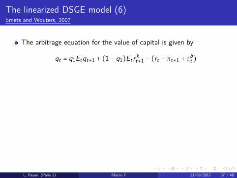
The linearized DSGE model (6)Smets and Wouters, 2007
The arbitrage equation for the value of capital is given by
qt = q1Etqt+1 + (1 − q1)Etrkt+1 − (rt − πt+1 + ε
bt )
The current value of the capital stock (qt) depends positively on itsexpected future value and the expected rental rate on capital (Etrk
t+1).And negatively on the ex-ante real interest rate and the risk premiumdisturbance.The aggregate production function is
yt = φp(αkst + (1 − α)lt + εa
t )
Output is produced using capital (kst ) and labor services (hours
worked lt).
L. Reyes (Paris 1) Macro 7 11/09/2017 37 / 48
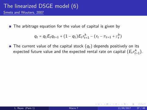
The linearized DSGE model (6)Smets and Wouters, 2007
The arbitrage equation for the value of capital is given by
qt = q1Etqt+1 + (1 − q1)Etrkt+1 − (rt − πt+1 + ε
bt )
The current value of the capital stock (qt) depends positively on itsexpected future value and the expected rental rate on capital (Etrk
t+1).
And negatively on the ex-ante real interest rate and the risk premiumdisturbance.The aggregate production function is
yt = φp(αkst + (1 − α)lt + εa
t )
Output is produced using capital (kst ) and labor services (hours
worked lt).
L. Reyes (Paris 1) Macro 7 11/09/2017 37 / 48
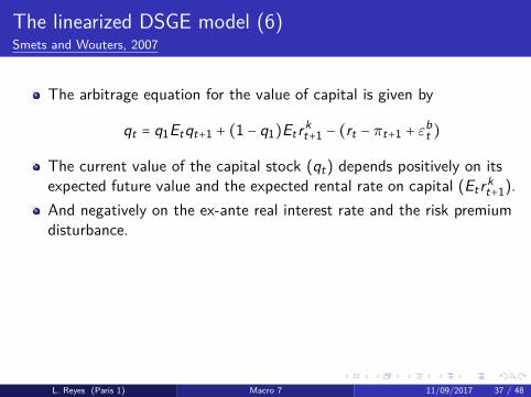
The linearized DSGE model (6)Smets and Wouters, 2007
The arbitrage equation for the value of capital is given by
qt = q1Etqt+1 + (1 − q1)Etrkt+1 − (rt − πt+1 + ε
bt )
The current value of the capital stock (qt) depends positively on itsexpected future value and the expected rental rate on capital (Etrk
t+1).And negatively on the ex-ante real interest rate and the risk premiumdisturbance.
The aggregate production function is
yt = φp(αkst + (1 − α)lt + εa
t )
Output is produced using capital (kst ) and labor services (hours
worked lt).
L. Reyes (Paris 1) Macro 7 11/09/2017 37 / 48
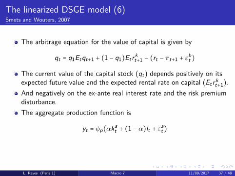
The linearized DSGE model (6)Smets and Wouters, 2007
The arbitrage equation for the value of capital is given by
qt = q1Etqt+1 + (1 − q1)Etrkt+1 − (rt − πt+1 + ε
bt )
The current value of the capital stock (qt) depends positively on itsexpected future value and the expected rental rate on capital (Etrk
t+1).And negatively on the ex-ante real interest rate and the risk premiumdisturbance.The aggregate production function is
yt = φp(αkst + (1 − α)lt + εa
t )
Output is produced using capital (kst ) and labor services (hours
worked lt).
L. Reyes (Paris 1) Macro 7 11/09/2017 37 / 48
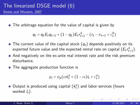
The linearized DSGE model (6)Smets and Wouters, 2007
The arbitrage equation for the value of capital is given by
qt = q1Etqt+1 + (1 − q1)Etrkt+1 − (rt − πt+1 + ε
bt )
The current value of the capital stock (qt) depends positively on itsexpected future value and the expected rental rate on capital (Etrk
t+1).And negatively on the ex-ante real interest rate and the risk premiumdisturbance.The aggregate production function is
yt = φp(αkst + (1 − α)lt + εa
t )
Output is produced using capital (kst ) and labor services (hours
worked lt).
L. Reyes (Paris 1) Macro 7 11/09/2017 37 / 48
The linearized DSGE model (7)Smets and Wouters, 2007
Total factor productivity (εat ) is assumed to follow an AR(1) process.
α captures the share of capital in production and φp is one plus theshare of fixed costs in production.As newly installed capital becomes only effective with a one-quarterlag, current capital services used in production (ks
t ) are a function ofcapital installed in the previous period (kt−1) and the degree ofcapital utilization
kst = kt−1 + zt
Cost minimization by the households that provide capital servicesimplies that zt is a positive function of the rental rate of capital
zt = z1rkt
L. Reyes (Paris 1) Macro 7 11/09/2017 38 / 48
The linearized DSGE model (7)Smets and Wouters, 2007
Total factor productivity (εat ) is assumed to follow an AR(1) process.
α captures the share of capital in production and φp is one plus theshare of fixed costs in production.
As newly installed capital becomes only effective with a one-quarterlag, current capital services used in production (ks
t ) are a function ofcapital installed in the previous period (kt−1) and the degree ofcapital utilization
kst = kt−1 + zt
Cost minimization by the households that provide capital servicesimplies that zt is a positive function of the rental rate of capital
zt = z1rkt
L. Reyes (Paris 1) Macro 7 11/09/2017 38 / 48
The linearized DSGE model (7)Smets and Wouters, 2007
Total factor productivity (εat ) is assumed to follow an AR(1) process.
α captures the share of capital in production and φp is one plus theshare of fixed costs in production.As newly installed capital becomes only effective with a one-quarterlag, current capital services used in production (ks
t ) are a function ofcapital installed in the previous period (kt−1) and the degree ofcapital utilization
kst = kt−1 + zt
Cost minimization by the households that provide capital servicesimplies that zt is a positive function of the rental rate of capital
zt = z1rkt
L. Reyes (Paris 1) Macro 7 11/09/2017 38 / 48
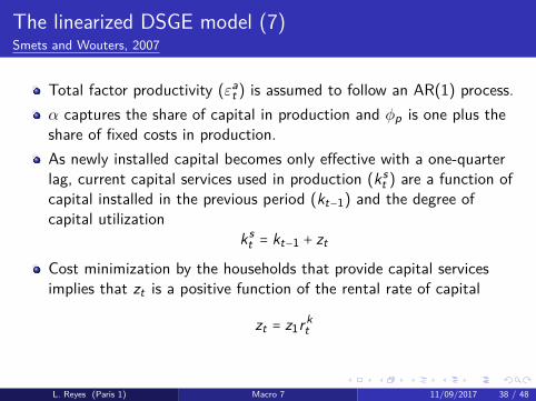
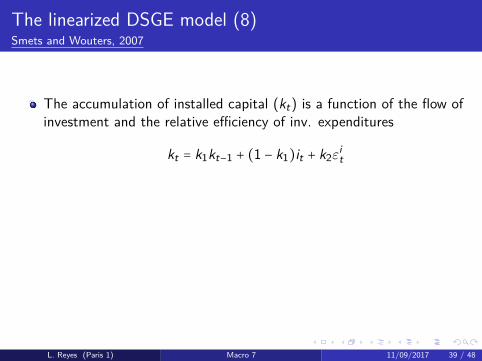
The linearized DSGE model (8)Smets and Wouters, 2007
The accumulation of installed capital (kt) is a function of the flow ofinvestment and the relative efficiency of inv. expenditures
kt = k1kt−1 + (1 − k1)it + k2εit
The price mark-up (µpt ) (difference between average price and
nominal marginal cost) equals the difference between the marginalproduct of labor (mplt) and the real wage (wt)
µpt = mplt −wt = α(ks
t − lt) + εat −wt
Prices adjust sluggishly to their desired mark-up.
L. Reyes (Paris 1) Macro 7 11/09/2017 39 / 48
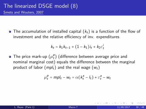
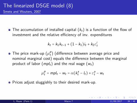
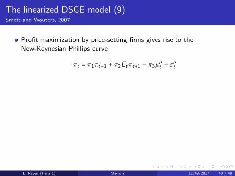
The linearized DSGE model (9)Smets and Wouters, 2007
Profit maximization by price-setting firms gives rise to theNew-Keynesian Phillips curve
πt = π1πt−1 + π2Etπt+1 − π3µpt + ε
pt
The price mark-up disturbance is assumed to follow an ARMA(1,1)process
εpt = ρpε
pt + η
pt − µpη
pt−1, with ηp
t ∼ i .i .d .
The assumption that all prices are indexed to either lagged inflationor the ss inflation ensures that the Phillips curve is vertical in thelong-run.Cost minimization by firms implies that the rental price of capital isnegatively associated to the capital-labor ratio and positively to thereal wage.
L. Reyes (Paris 1) Macro 7 11/09/2017 40 / 48
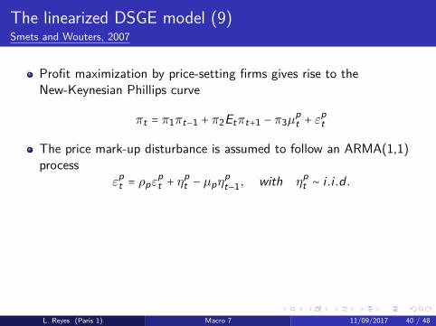
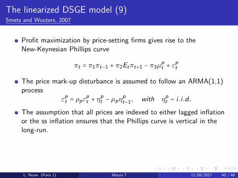
The linearized DSGE model (9)Smets and Wouters, 2007
Profit maximization by price-setting firms gives rise to theNew-Keynesian Phillips curve
πt = π1πt−1 + π2Etπt+1 − π3µpt + ε
pt
The price mark-up disturbance is assumed to follow an ARMA(1,1)process
εpt = ρpε
pt + η
pt − µpη
pt−1, with ηp
t ∼ i .i .d .
The assumption that all prices are indexed to either lagged inflationor the ss inflation ensures that the Phillips curve is vertical in thelong-run.
Cost minimization by firms implies that the rental price of capital isnegatively associated to the capital-labor ratio and positively to thereal wage.
L. Reyes (Paris 1) Macro 7 11/09/2017 40 / 48
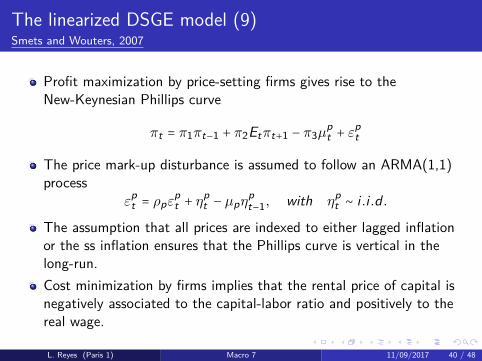
The linearized DSGE model (9)Smets and Wouters, 2007
Profit maximization by price-setting firms gives rise to theNew-Keynesian Phillips curve
πt = π1πt−1 + π2Etπt+1 − π3µpt + ε
pt
The price mark-up disturbance is assumed to follow an ARMA(1,1)process
εpt = ρpε
pt + η
pt − µpη
pt−1, with ηp
t ∼ i .i .d .
The assumption that all prices are indexed to either lagged inflationor the ss inflation ensures that the Phillips curve is vertical in thelong-run.Cost minimization by firms implies that the rental price of capital isnegatively associated to the capital-labor ratio and positively to thereal wage.
L. Reyes (Paris 1) Macro 7 11/09/2017 40 / 48
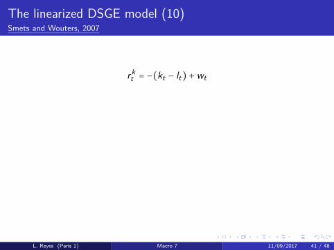
The linearized DSGE model (10)Smets and Wouters, 2007
rkt = −(kt − lt) +wt
Due to nominal wage stickiness and partial indexation of wages toinflation, real wages only adjust gradually to the desired mark-up
wt = w1wt−1 + (1−w1)(Etwt+1 +Etφt+1)−w2πt +w3πt−1 −w4µwt + εw
t
If wages are perfectly flexible, the real wage is a constant mark-upover the marginal rate of substitution between consumption andleisure.The wage mark-up disturbance follows an ARMA(1,1) process.
L. Reyes (Paris 1) Macro 7 11/09/2017 41 / 48
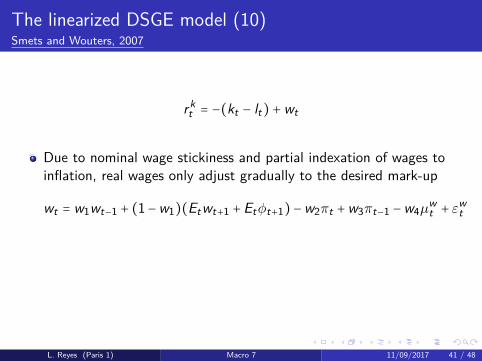
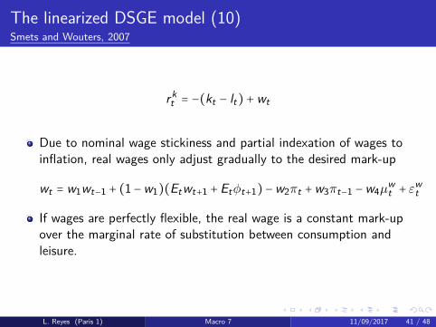
The linearized DSGE model (10)Smets and Wouters, 2007
rkt = −(kt − lt) +wt
Due to nominal wage stickiness and partial indexation of wages toinflation, real wages only adjust gradually to the desired mark-up
wt = w1wt−1 + (1−w1)(Etwt+1 +Etφt+1)−w2πt +w3πt−1 −w4µwt + εw
t
If wages are perfectly flexible, the real wage is a constant mark-upover the marginal rate of substitution between consumption andleisure.
The wage mark-up disturbance follows an ARMA(1,1) process.
L. Reyes (Paris 1) Macro 7 11/09/2017 41 / 48
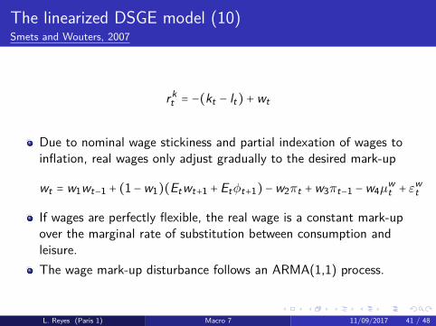
The linearized DSGE model (10)Smets and Wouters, 2007
rkt = −(kt − lt) +wt
Due to nominal wage stickiness and partial indexation of wages toinflation, real wages only adjust gradually to the desired mark-up
wt = w1wt−1 + (1−w1)(Etwt+1 +Etφt+1)−w2πt +w3πt−1 −w4µwt + εw
t
If wages are perfectly flexible, the real wage is a constant mark-upover the marginal rate of substitution between consumption andleisure.The wage mark-up disturbance follows an ARMA(1,1) process.
L. Reyes (Paris 1) Macro 7 11/09/2017 41 / 48
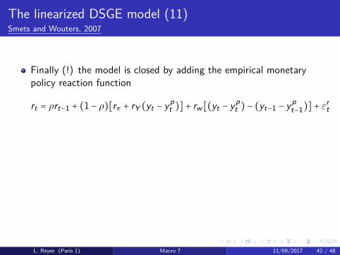
The linearized DSGE model (11)Smets and Wouters, 2007
Finally (!) the model is closed by adding the empirical monetarypolicy reaction function
rt = ρrt−1 + (1− ρ)[rπ + rY (yt − ypt )]+ rw [(yt − yp
t )− (yt−1 − ypt−1)]+ ε
rt
We assume that the monetary policy shocks (εrt) follows an AR(1)
process with i.i.d. error term (εrt = ρRε
rt−1 + η
rt ).
The stochastic behavior of the system of linear rational expectationsequations is driven by seven exogenous disturbances:
(1) total factorproductivity (εa
t ), (2) investment-specific technology (εit), (3) risk
premium (εbt ), (4) exogenous spending (εg
t ), (5) price mark-up (εpt ),
(6) wage mark-up (εwt ) and (7) monetary policy shocks (εr
t).
L. Reyes (Paris 1) Macro 7 11/09/2017 42 / 48
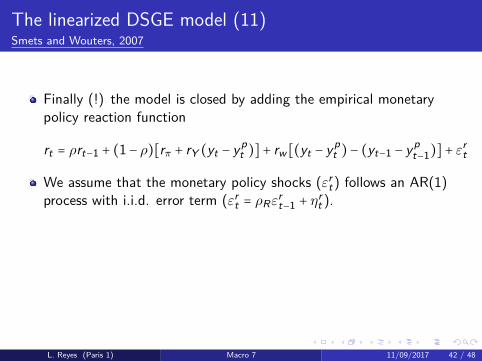
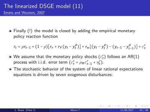
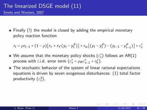
The linearized DSGE model (11)Smets and Wouters, 2007
Finally (!) the model is closed by adding the empirical monetarypolicy reaction function
rt = ρrt−1 + (1− ρ)[rπ + rY (yt − ypt )]+ rw [(yt − yp
t )− (yt−1 − ypt−1)]+ ε
rt
We assume that the monetary policy shocks (εrt) follows an AR(1)
process with i.i.d. error term (εrt = ρRε
rt−1 + η
rt ).
The stochastic behavior of the system of linear rational expectationsequations is driven by seven exogenous disturbances: (1) total factorproductivity (εa
t ),
(2) investment-specific technology (εit), (3) risk
premium (εbt ), (4) exogenous spending (εg
t ), (5) price mark-up (εpt ),
(6) wage mark-up (εwt ) and (7) monetary policy shocks (εr
t).
L. Reyes (Paris 1) Macro 7 11/09/2017 42 / 48
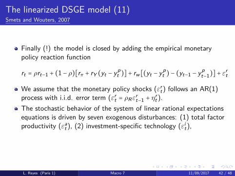
The linearized DSGE model (11)Smets and Wouters, 2007
Finally (!) the model is closed by adding the empirical monetarypolicy reaction function
rt = ρrt−1 + (1− ρ)[rπ + rY (yt − ypt )]+ rw [(yt − yp
t )− (yt−1 − ypt−1)]+ ε
rt
We assume that the monetary policy shocks (εrt) follows an AR(1)
process with i.i.d. error term (εrt = ρRε
rt−1 + η
rt ).
The stochastic behavior of the system of linear rational expectationsequations is driven by seven exogenous disturbances: (1) total factorproductivity (εa
t ), (2) investment-specific technology (εit),
(3) riskpremium (εb
t ), (4) exogenous spending (εgt ), (5) price mark-up (εp
t ),(6) wage mark-up (εw
t ) and (7) monetary policy shocks (εrt).
L. Reyes (Paris 1) Macro 7 11/09/2017 42 / 48
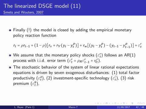
The linearized DSGE model (11)Smets and Wouters, 2007
Finally (!) the model is closed by adding the empirical monetarypolicy reaction function
rt = ρrt−1 + (1− ρ)[rπ + rY (yt − ypt )]+ rw [(yt − yp
t )− (yt−1 − ypt−1)]+ ε
rt
We assume that the monetary policy shocks (εrt) follows an AR(1)
process with i.i.d. error term (εrt = ρRε
rt−1 + η
rt ).
The stochastic behavior of the system of linear rational expectationsequations is driven by seven exogenous disturbances: (1) total factorproductivity (εa
t ), (2) investment-specific technology (εit), (3) risk
premium (εbt ),
(4) exogenous spending (εgt ), (5) price mark-up (εp
t ),(6) wage mark-up (εw
t ) and (7) monetary policy shocks (εrt).
L. Reyes (Paris 1) Macro 7 11/09/2017 42 / 48
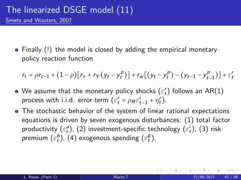
The linearized DSGE model (11)Smets and Wouters, 2007
Finally (!) the model is closed by adding the empirical monetarypolicy reaction function
rt = ρrt−1 + (1− ρ)[rπ + rY (yt − ypt )]+ rw [(yt − yp
t )− (yt−1 − ypt−1)]+ ε
rt
We assume that the monetary policy shocks (εrt) follows an AR(1)
process with i.i.d. error term (εrt = ρRε
rt−1 + η
rt ).
The stochastic behavior of the system of linear rational expectationsequations is driven by seven exogenous disturbances: (1) total factorproductivity (εa
t ), (2) investment-specific technology (εit), (3) risk
premium (εbt ), (4) exogenous spending (εg
t ),
(5) price mark-up (εpt ),
(6) wage mark-up (εwt ) and (7) monetary policy shocks (εr
t).
L. Reyes (Paris 1) Macro 7 11/09/2017 42 / 48
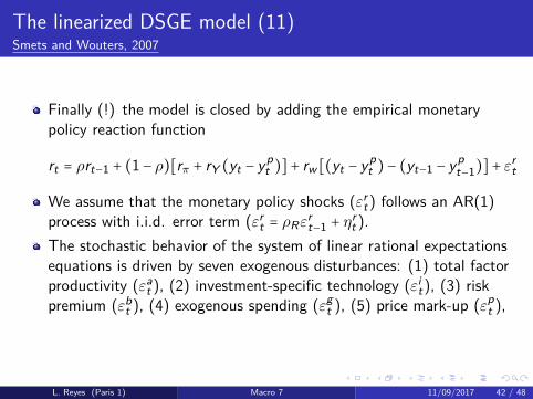
The linearized DSGE model (11)Smets and Wouters, 2007
Finally (!) the model is closed by adding the empirical monetarypolicy reaction function
rt = ρrt−1 + (1− ρ)[rπ + rY (yt − ypt )]+ rw [(yt − yp
t )− (yt−1 − ypt−1)]+ ε
rt
We assume that the monetary policy shocks (εrt) follows an AR(1)
process with i.i.d. error term (εrt = ρRε
rt−1 + η
rt ).
The stochastic behavior of the system of linear rational expectationsequations is driven by seven exogenous disturbances: (1) total factorproductivity (εa
t ), (2) investment-specific technology (εit), (3) risk
premium (εbt ), (4) exogenous spending (εg
t ), (5) price mark-up (εpt ),
(6) wage mark-up (εwt ) and (7) monetary policy shocks (εr
t).
L. Reyes (Paris 1) Macro 7 11/09/2017 42 / 48
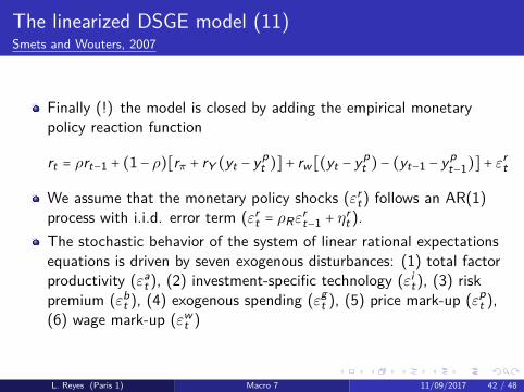
The linearized DSGE model (11)Smets and Wouters, 2007
Finally (!) the model is closed by adding the empirical monetarypolicy reaction function
rt = ρrt−1 + (1− ρ)[rπ + rY (yt − ypt )]+ rw [(yt − yp
t )− (yt−1 − ypt−1)]+ ε
rt
We assume that the monetary policy shocks (εrt) follows an AR(1)
process with i.i.d. error term (εrt = ρRε
rt−1 + η
rt ).
The stochastic behavior of the system of linear rational expectationsequations is driven by seven exogenous disturbances: (1) total factorproductivity (εa
t ), (2) investment-specific technology (εit), (3) risk
premium (εbt ), (4) exogenous spending (εg
t ), (5) price mark-up (εpt ),
(6) wage mark-up (εwt )
and (7) monetary policy shocks (εrt).
L. Reyes (Paris 1) Macro 7 11/09/2017 42 / 48
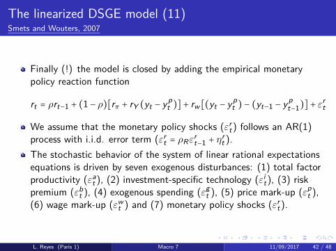
The linearized DSGE model (11)Smets and Wouters, 2007
Finally (!) the model is closed by adding the empirical monetarypolicy reaction function
rt = ρrt−1 + (1− ρ)[rπ + rY (yt − ypt )]+ rw [(yt − yp
t )− (yt−1 − ypt−1)]+ ε
rt
We assume that the monetary policy shocks (εrt) follows an AR(1)
process with i.i.d. error term (εrt = ρRε
rt−1 + η
rt ).
The stochastic behavior of the system of linear rational expectationsequations is driven by seven exogenous disturbances: (1) total factorproductivity (εa
t ), (2) investment-specific technology (εit), (3) risk
premium (εbt ), (4) exogenous spending (εg
t ), (5) price mark-up (εpt ),
(6) wage mark-up (εwt ) and (7) monetary policy shocks (εr
t).
L. Reyes (Paris 1) Macro 7 11/09/2017 42 / 48

Outline
1 Real Business CyclesIntroductionBusiness cycle phenomena and growth modelUsing data to restrict the growth model, i.e. calibration
2 Dynamic Stochastic General Equilibrium modelsIntroductionThe linearized DSGE modelParameter estimates and model properties
L. Reyes (Paris 1) Macro 7 11/09/2017 43 / 48
Parameter estimates and model properties (1)Smets and Wouters, 2007
The model is estimated with Bayesian estimation techniques using sevenkey macroeconomic quarterly U.S. time series:
log difference of real GDP (dlGDPt),log difference of real consumption (dlCONSt),log difference of real investment (dlINVt),log difference of the real wage (dlWAGt),log hours worked (lHOURSt),log difference of GDP deflator (dlPt),and the federal funds rate (FEDFUNDSt).
L. Reyes (Paris 1) Macro 7 11/09/2017 44 / 48
Parameter estimates and model properties (1)Smets and Wouters, 2007
The model is estimated with Bayesian estimation techniques using sevenkey macroeconomic quarterly U.S. time series:
log difference of real GDP (dlGDPt),
log difference of real consumption (dlCONSt),log difference of real investment (dlINVt),log difference of the real wage (dlWAGt),log hours worked (lHOURSt),log difference of GDP deflator (dlPt),and the federal funds rate (FEDFUNDSt).
L. Reyes (Paris 1) Macro 7 11/09/2017 44 / 48
Parameter estimates and model properties (1)Smets and Wouters, 2007
The model is estimated with Bayesian estimation techniques using sevenkey macroeconomic quarterly U.S. time series:
log difference of real GDP (dlGDPt),log difference of real consumption (dlCONSt),
log difference of real investment (dlINVt),log difference of the real wage (dlWAGt),log hours worked (lHOURSt),log difference of GDP deflator (dlPt),and the federal funds rate (FEDFUNDSt).
L. Reyes (Paris 1) Macro 7 11/09/2017 44 / 48
Parameter estimates and model properties (1)Smets and Wouters, 2007
The model is estimated with Bayesian estimation techniques using sevenkey macroeconomic quarterly U.S. time series:
log difference of real GDP (dlGDPt),log difference of real consumption (dlCONSt),log difference of real investment (dlINVt),
log difference of the real wage (dlWAGt),log hours worked (lHOURSt),log difference of GDP deflator (dlPt),and the federal funds rate (FEDFUNDSt).
L. Reyes (Paris 1) Macro 7 11/09/2017 44 / 48
Parameter estimates and model properties (1)Smets and Wouters, 2007
The model is estimated with Bayesian estimation techniques using sevenkey macroeconomic quarterly U.S. time series:
log difference of real GDP (dlGDPt),log difference of real consumption (dlCONSt),log difference of real investment (dlINVt),log difference of the real wage (dlWAGt),
log hours worked (lHOURSt),log difference of GDP deflator (dlPt),and the federal funds rate (FEDFUNDSt).
L. Reyes (Paris 1) Macro 7 11/09/2017 44 / 48
Parameter estimates and model properties (1)Smets and Wouters, 2007
The model is estimated with Bayesian estimation techniques using sevenkey macroeconomic quarterly U.S. time series:
log difference of real GDP (dlGDPt),log difference of real consumption (dlCONSt),log difference of real investment (dlINVt),log difference of the real wage (dlWAGt),log hours worked (lHOURSt),
log difference of GDP deflator (dlPt),and the federal funds rate (FEDFUNDSt).
L. Reyes (Paris 1) Macro 7 11/09/2017 44 / 48
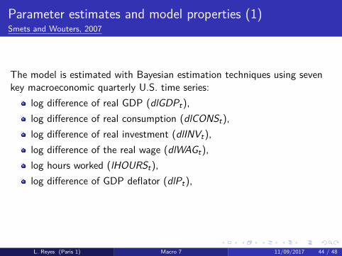
Parameter estimates and model properties (1)Smets and Wouters, 2007
The model is estimated with Bayesian estimation techniques using sevenkey macroeconomic quarterly U.S. time series:
log difference of real GDP (dlGDPt),log difference of real consumption (dlCONSt),log difference of real investment (dlINVt),log difference of the real wage (dlWAGt),log hours worked (lHOURSt),log difference of GDP deflator (dlPt),
and the federal funds rate (FEDFUNDSt).
L. Reyes (Paris 1) Macro 7 11/09/2017 44 / 48
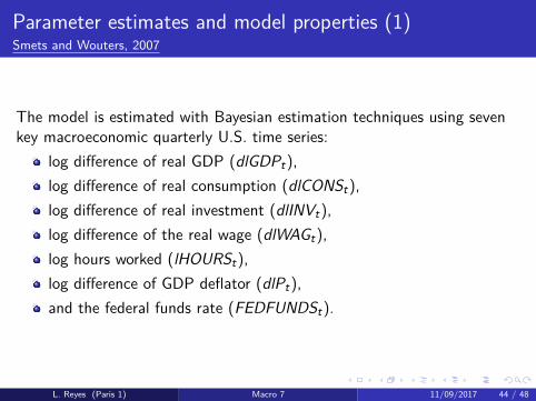
Parameter estimates and model properties (1)Smets and Wouters, 2007
The model is estimated with Bayesian estimation techniques using sevenkey macroeconomic quarterly U.S. time series:
log difference of real GDP (dlGDPt),log difference of real consumption (dlCONSt),log difference of real investment (dlINVt),log difference of the real wage (dlWAGt),log hours worked (lHOURSt),log difference of GDP deflator (dlPt),and the federal funds rate (FEDFUNDSt).
L. Reyes (Paris 1) Macro 7 11/09/2017 44 / 48
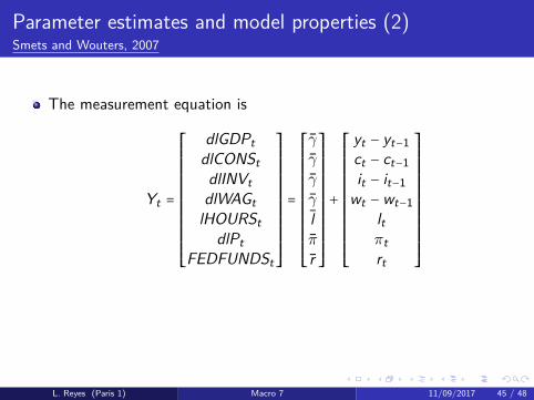
Parameter estimates and model properties (2)Smets and Wouters, 2007
The measurement equation is
Yt =
⎡⎢⎢⎢⎢⎢⎢⎢⎢⎢⎢⎢⎢⎢⎢⎣
dlGDPtdlCONStdlINVtdlWAGtlHOURSt
dlPtFEDFUNDSt
⎤⎥⎥⎥⎥⎥⎥⎥⎥⎥⎥⎥⎥⎥⎥⎦
=
⎡⎢⎢⎢⎢⎢⎢⎢⎢⎢⎢⎢⎢⎢⎢⎣
γγγγ
lπr
⎤⎥⎥⎥⎥⎥⎥⎥⎥⎥⎥⎥⎥⎥⎥⎦
+
⎡⎢⎢⎢⎢⎢⎢⎢⎢⎢⎢⎢⎢⎢⎢⎣
yt − yt−1ct − ct−1it − it−1wt −wt−1
ltπtrt
⎤⎥⎥⎥⎥⎥⎥⎥⎥⎥⎥⎥⎥⎥⎥⎦
γ = 100(γ − 1) is the common quarterly trend growth rate to realGDP, consumption, investment and wages, π = 100(Π∗ − 1) is thequarterly ss inflation rate and r = 100(β−1γσc Π∗ − 1).
L. Reyes (Paris 1) Macro 7 11/09/2017 45 / 48
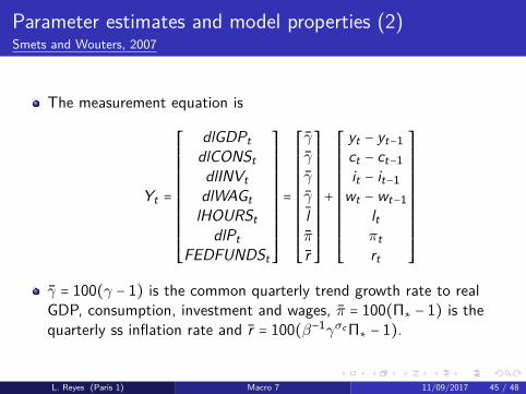
Parameter estimates and model properties (3)Smets and Wouters, 2007
The model is estimated for 1966q1 - 2004q4, as well as the "GreatInflation" (1966q1 - 1979q2) and the "Great Moderation" (1984q1 -2004q4).
The authors distinguish between priors on the stochastic processes(assumed distributions of the disturbance terms) and posteriorestimates (estimated values obtained after assumptions).SW mention that their tightly parameterized DSGE model performsmuch better than an unconstrained VAR in the same vector ofobservable variables.It can also compete with standard BVAR models (Sims and Zha,1998) in terms of empirical one-step-ahead prediction performance.
L. Reyes (Paris 1) Macro 7 11/09/2017 46 / 48
Parameter estimates and model properties (3)Smets and Wouters, 2007
The model is estimated for 1966q1 - 2004q4, as well as the "GreatInflation" (1966q1 - 1979q2) and the "Great Moderation" (1984q1 -2004q4).The authors distinguish between priors on the stochastic processes(assumed distributions of the disturbance terms) and posteriorestimates (estimated values obtained after assumptions).
SW mention that their tightly parameterized DSGE model performsmuch better than an unconstrained VAR in the same vector ofobservable variables.It can also compete with standard BVAR models (Sims and Zha,1998) in terms of empirical one-step-ahead prediction performance.
L. Reyes (Paris 1) Macro 7 11/09/2017 46 / 48
Parameter estimates and model properties (3)Smets and Wouters, 2007
The model is estimated for 1966q1 - 2004q4, as well as the "GreatInflation" (1966q1 - 1979q2) and the "Great Moderation" (1984q1 -2004q4).The authors distinguish between priors on the stochastic processes(assumed distributions of the disturbance terms) and posteriorestimates (estimated values obtained after assumptions).SW mention that their tightly parameterized DSGE model performsmuch better than an unconstrained VAR in the same vector ofobservable variables.
It can also compete with standard BVAR models (Sims and Zha,1998) in terms of empirical one-step-ahead prediction performance.
L. Reyes (Paris 1) Macro 7 11/09/2017 46 / 48
Parameter estimates and model properties (3)Smets and Wouters, 2007
The model is estimated for 1966q1 - 2004q4, as well as the "GreatInflation" (1966q1 - 1979q2) and the "Great Moderation" (1984q1 -2004q4).The authors distinguish between priors on the stochastic processes(assumed distributions of the disturbance terms) and posteriorestimates (estimated values obtained after assumptions).SW mention that their tightly parameterized DSGE model performsmuch better than an unconstrained VAR in the same vector ofobservable variables.It can also compete with standard BVAR models (Sims and Zha,1998) in terms of empirical one-step-ahead prediction performance.
L. Reyes (Paris 1) Macro 7 11/09/2017 46 / 48
Main driving forces of output (1)Smets and Wouters, 2007
In the short run, movements in GDP are primarily driven by theexogenous spending shock and the two shocks that affect theintertemporal Euler equations:
The risk premium shock which affects both consumption andinvestment, andThe investment-specific technology shock which affects theinvestment Euler equation.These are demand shocks that have a positive effect on output,hours worked, inflation and the nominal interest rate under theestimated policy rule.However, it is mostly two supply shocks that account for most of theoutput variations in the medium to long run:
productivity and wagemark-up.
L. Reyes (Paris 1) Macro 7 11/09/2017 47 / 48
Main driving forces of output (1)Smets and Wouters, 2007
In the short run, movements in GDP are primarily driven by theexogenous spending shock and the two shocks that affect theintertemporal Euler equations:The risk premium shock which affects both consumption andinvestment, and
The investment-specific technology shock which affects theinvestment Euler equation.These are demand shocks that have a positive effect on output,hours worked, inflation and the nominal interest rate under theestimated policy rule.However, it is mostly two supply shocks that account for most of theoutput variations in the medium to long run:
productivity and wagemark-up.
L. Reyes (Paris 1) Macro 7 11/09/2017 47 / 48
Main driving forces of output (1)Smets and Wouters, 2007
In the short run, movements in GDP are primarily driven by theexogenous spending shock and the two shocks that affect theintertemporal Euler equations:The risk premium shock which affects both consumption andinvestment, andThe investment-specific technology shock which affects theinvestment Euler equation.
These are demand shocks that have a positive effect on output,hours worked, inflation and the nominal interest rate under theestimated policy rule.However, it is mostly two supply shocks that account for most of theoutput variations in the medium to long run:
productivity and wagemark-up.
L. Reyes (Paris 1) Macro 7 11/09/2017 47 / 48
Main driving forces of output (1)Smets and Wouters, 2007
In the short run, movements in GDP are primarily driven by theexogenous spending shock and the two shocks that affect theintertemporal Euler equations:The risk premium shock which affects both consumption andinvestment, andThe investment-specific technology shock which affects theinvestment Euler equation.These are demand shocks that have a positive effect on output,hours worked, inflation and the nominal interest rate under theestimated policy rule.
However, it is mostly two supply shocks that account for most of theoutput variations in the medium to long run:
productivity and wagemark-up.
L. Reyes (Paris 1) Macro 7 11/09/2017 47 / 48

Main driving forces of output (1)Smets and Wouters, 2007
In the short run, movements in GDP are primarily driven by theexogenous spending shock and the two shocks that affect theintertemporal Euler equations:The risk premium shock which affects both consumption andinvestment, andThe investment-specific technology shock which affects theinvestment Euler equation.These are demand shocks that have a positive effect on output,hours worked, inflation and the nominal interest rate under theestimated policy rule.However, it is mostly two supply shocks that account for most of theoutput variations in the medium to long run:
productivity and wagemark-up.
L. Reyes (Paris 1) Macro 7 11/09/2017 47 / 48
Main driving forces of output (1)Smets and Wouters, 2007
In the short run, movements in GDP are primarily driven by theexogenous spending shock and the two shocks that affect theintertemporal Euler equations:The risk premium shock which affects both consumption andinvestment, andThe investment-specific technology shock which affects theinvestment Euler equation.These are demand shocks that have a positive effect on output,hours worked, inflation and the nominal interest rate under theestimated policy rule.However, it is mostly two supply shocks that account for most of theoutput variations in the medium to long run: productivity and wagemark-up.
L. Reyes (Paris 1) Macro 7 11/09/2017 47 / 48

Last slide
End of the seventh lecture.
L. Reyes (Paris 1) Macro 7 11/09/2017 48 / 48