Macroeconomics - ECO 2013

2004 Summer Term BJune 21 – July 30, 2004

Lecture 9: Monday, July 12th

Review Quiz 3 on Chapters 7 & 8Review Mid-term Progress Reports

Class AttendanceExtra Credit: Attend FTAA DebateChapter 9: Building the Aggregate Expenditures ModelChapter 10: Aggregate ExpendituresNext Class on Wednesday, July 14th

Review Quiz 3 on Chapters 7 & 8

Worth 20 points> 15 points: 16 students10 – 15 points: 4 students< 10 points: 3 students

Range 1.5 – 29.50

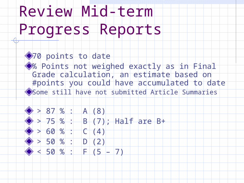
Review Mid-term Progress Reports

70 points to date% Points not weighed exactly as in Final Grade calculation, an estimate based on #points you could have accumulated to dateSome still have not submitted Article Summaries

> 87 % : A (8) > 75 % : B (7); Half are B+ > 60 % : C (4) > 50 % : D (2) < 50 % : F (5 – 7)

Class Attendance

Extra Credit Attend FTAA Debate

Thursday, July 15th

3:30 – 7:00 PMFIU University Park Campus: MARC Pavilion CenterCost: $15

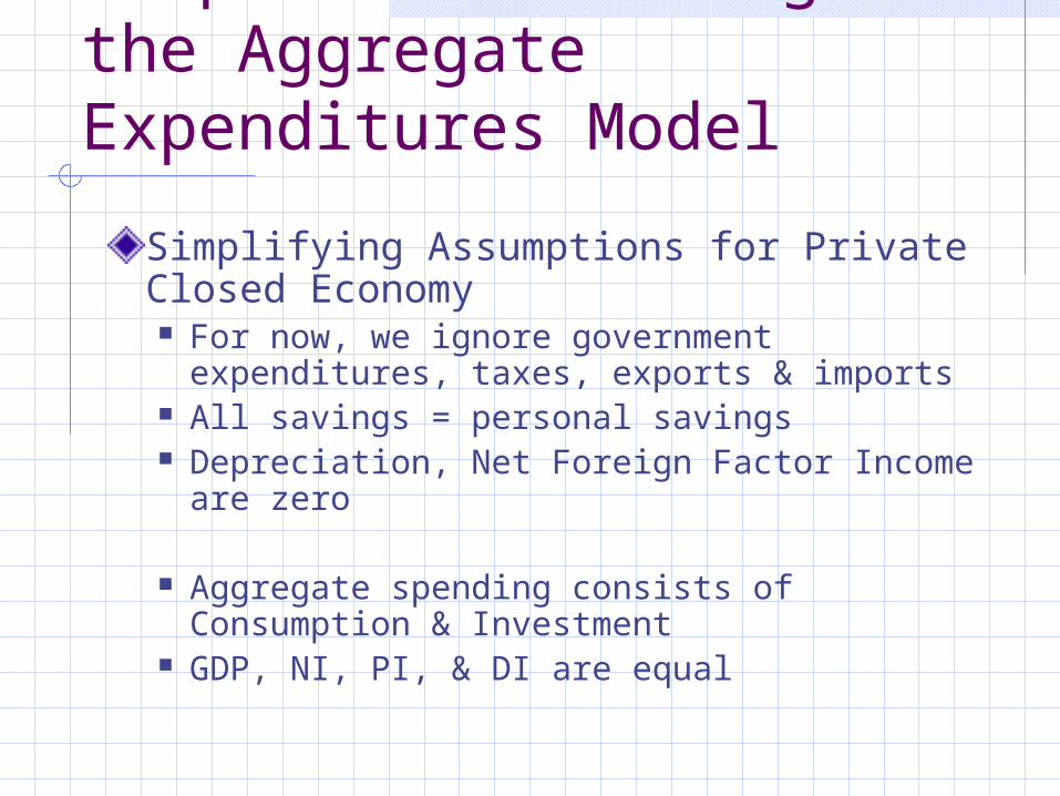
Chapter 9: Building the Aggregate Expenditures Model

Simplifying Assumptions for Private Closed Economy For now, we ignore government

expenditures, taxes, exports & imports All savings = personal savings Depreciation, Net Foreign Factor Income are

zero

Aggregate spending consists of Consumption & Investment

GDP, NI, PI, & DI are equal

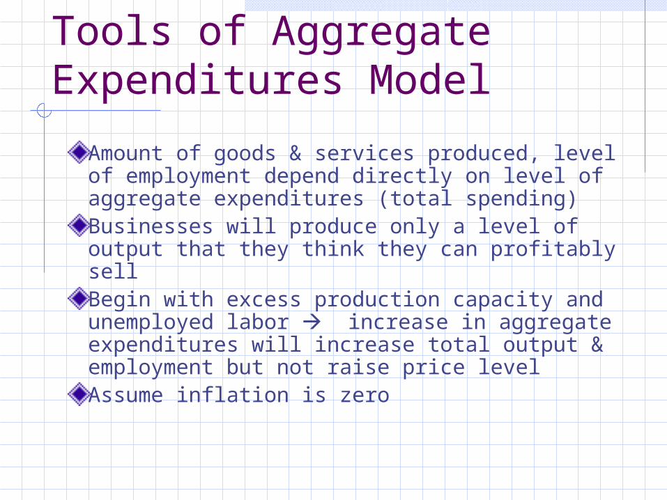
Tools of Aggregate Expenditures Model

Amount of goods & services produced, level of employment depend directly on level of aggregate expenditures (total spending)Businesses will produce only a level of output that they think they can profitably sellBegin with excess production capacity and unemployed labor increase in aggregate expenditures will increase total output & employment but not raise price levelAssume inflation is zero

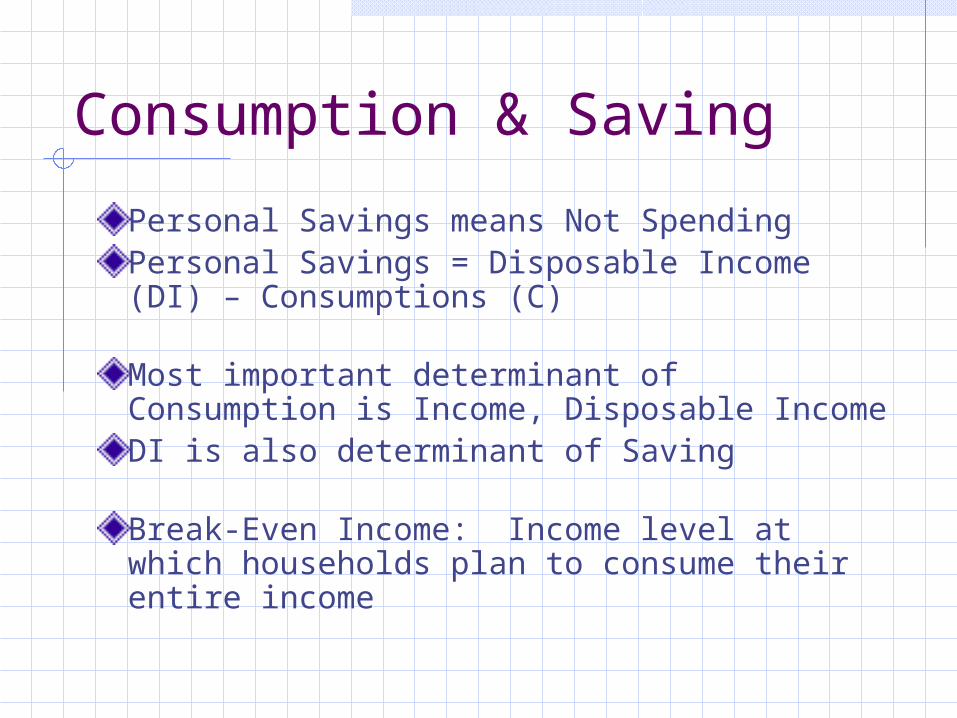
Consumption & Saving

Personal Savings means Not SpendingPersonal Savings = Disposable Income (DI) – Consumptions (C)

Most important determinant of Consumption is Income, Disposable IncomeDI is also determinant of Saving

Break-Even Income: Income level at which households plan to consume their entire income

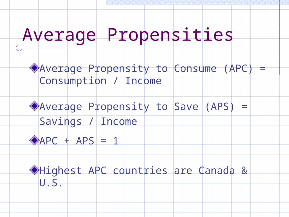
Average Propensities

Average Propensity to Consume (APC) = Consumption / Income

Average Propensity to Save (APS) = Savings / Income

APC + APS = 1

Highest APC countries are Canada & U.S.

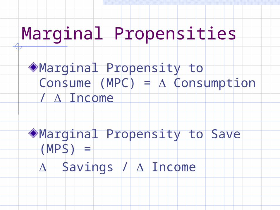
Marginal Propensities

Marginal Propensity to Consume (MPC) = Consumption / Income

Marginal Propensity to Save (MPS) = Savings / Income

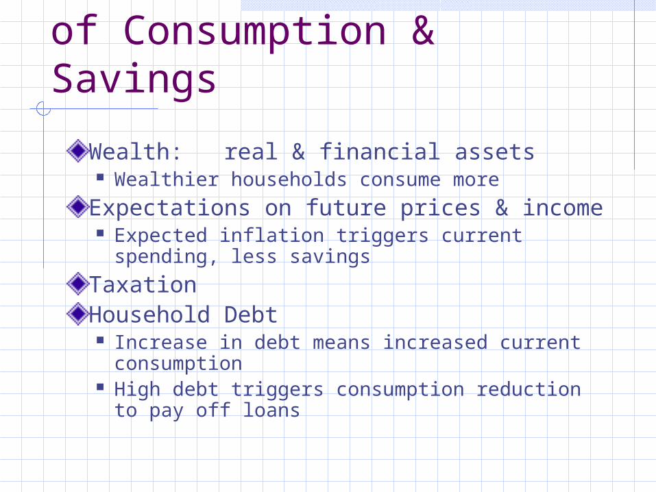
Nonincome Determinants of Consumption & Savings

Wealth: real & financial assets Wealthier households consume more

Expectations on future prices & income Expected inflation triggers current spending,

less savings

TaxationHousehold Debt Increase in debt means increased current

consumption High debt triggers consumption reduction to

pay off loans

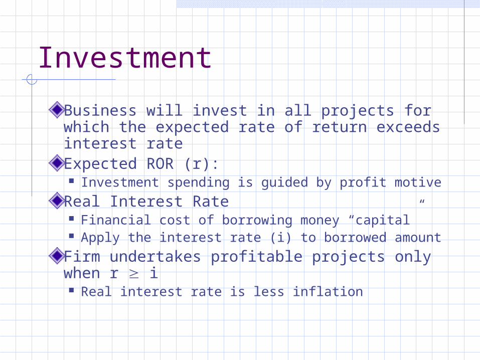
Investment

Business will invest in all projects for which the expected rate of return exceeds interest rateExpected ROR (r): Investment spending is guided by profit motive

Real Interest Rate Financial cost of borrowing money “capital” Apply the interest rate (i) to borrowed amount

Firm undertakes profitable projects only when r i Real interest rate is less inflation

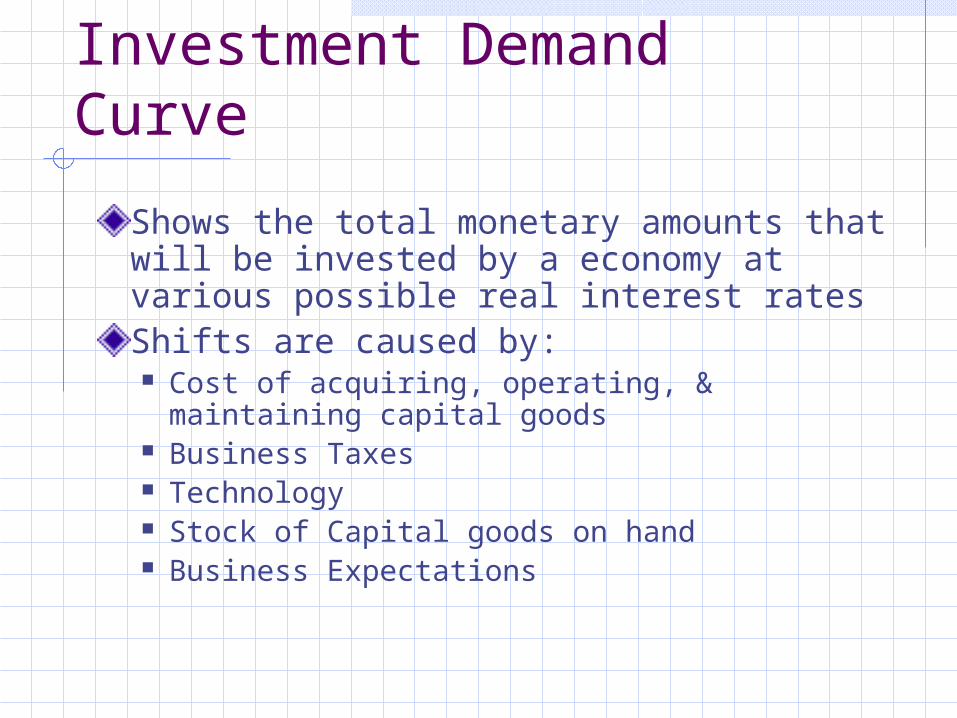
Investment Demand Curve

Shows the total monetary amounts that will be invested by a economy at various possible real interest ratesShifts are caused by: Cost of acquiring, operating, & maintaining

capital goods Business Taxes Technology Stock of Capital goods on hand Business Expectations

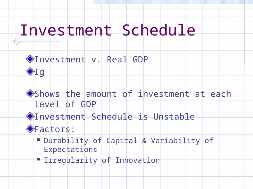
Investment Schedule

Investment v. Real GDPIg

Shows the amount of investment at each level of GDPInvestment Schedule is UnstableFactors: Durability of Capital & Variability of Expectations Irregularity of Innovation

Equilibrium GDP

In closed economy, aggregate expenditures (GDP) consist only of consumption (C) + investment (Ig) Total level of goods produced = C + Ig

Equilibrium Output: Output whose production creates total spending just sufficient to purchase that output No overproduction No excess of total spending

At Equilibrium GDP, C + Ig = GDP

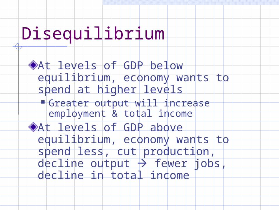
Disequilibrium

At levels of GDP below equilibrium, economy wants to spend at higher levels Greater output will increase

employment & total income

At levels of GDP above equilibrium, economy wants to spend less, cut production, decline output fewer jobs, decline in total income

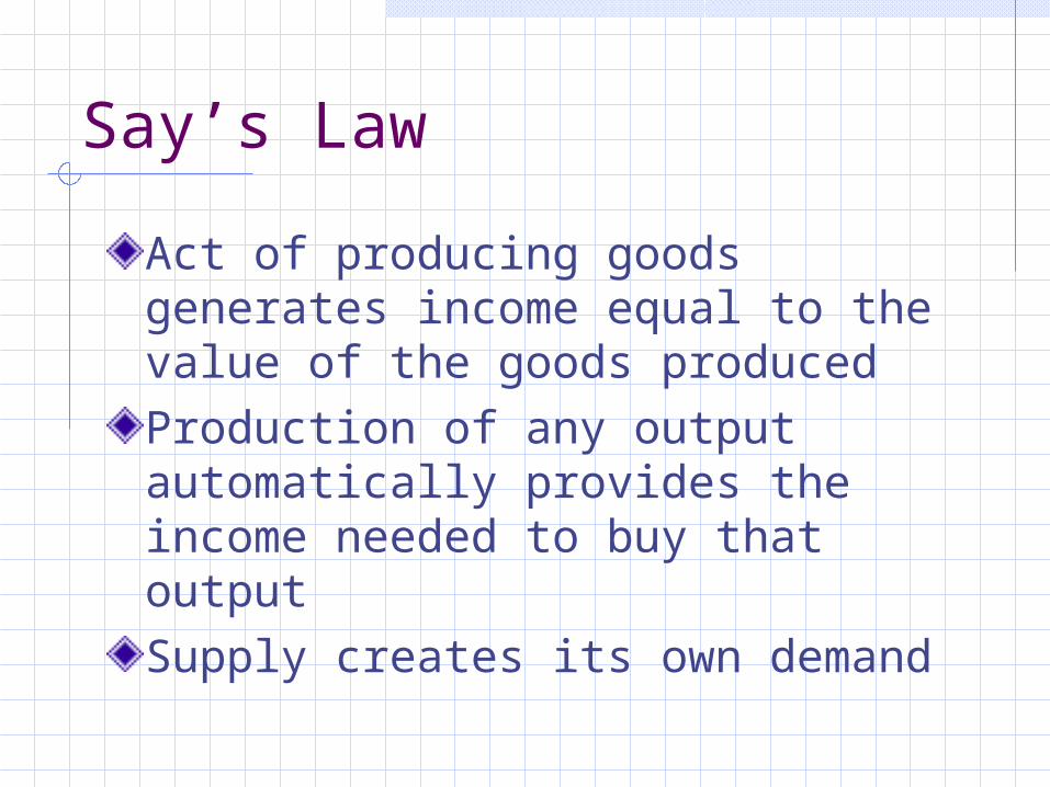
Say’s Law

Act of producing goods generates income equal to the value of the goods producedProduction of any output automatically provides the income needed to buy that outputSupply creates its own demand

Chapter 10: Aggregate Expenditures

Net ExportsGovernment

International Trade & Equilibrium Output

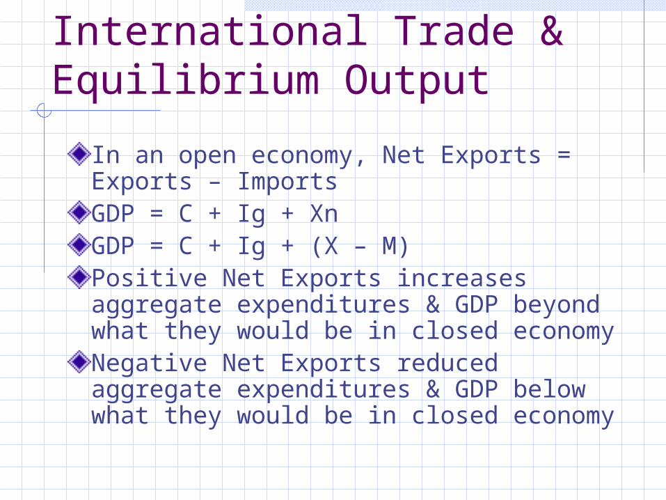
In an open economy, Net Exports = Exports – ImportsGDP = C + Ig + XnGDP = C + Ig + (X – M) Positive Net Exports increases aggregate expenditures & GDP beyond what they would be in closed economyNegative Net Exports reduced aggregate expenditures & GDP below what they would be in closed economy

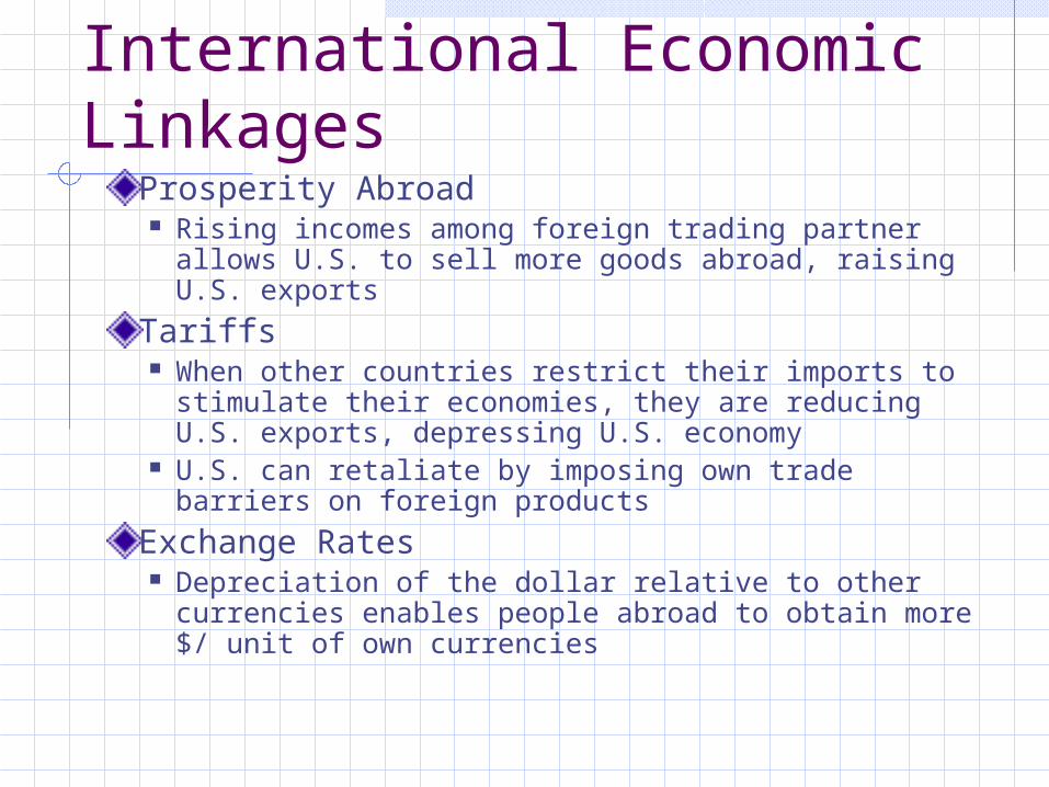
International Economic Linkages

Prosperity Abroad Rising incomes among foreign trading partner

allows U.S. to sell more goods abroad, raising U.S. exports

Tariffs When other countries restrict their imports to

stimulate their economies, they are reducing U.S. exports, depressing U.S. economy

U.S. can retaliate by imposing own trade barriers on foreign products

Exchange Rates Depreciation of the dollar relative to other

currencies enables people abroad to obtain more $/ unit of own currencies

Government

Add government spending and taxes to modelSimplifying Assumptions Levels of investment & net exports are

independent of level of GDP Gov’t purchases can’t affect private spending Gov’t tax revenues

Disposable Income < Personal Income GDP, NI, PI remain equal Fixed taxes are collected No inflation

Next Class on Wednesday, July 14th

Chapters 11, 12 & 16Review Progress ReportsThird Article Summaries Due