Embed Size (px)
Citation preview
MACROECONOMICS
© 2013 Worth Publishers, all rights reserved
PowerPoint ® Slides by Ron Cronovich
N. Gregory Mankiw
Economic Growth II:Technology, Empirics, and Policy
9
IN THIS CHAPTER, YOU WILL LEARN:
how to incorporate technological progress in the Solow model
about policies to promote growth
about growth empirics: confronting the theory with facts
two simple models in which the rate of technological progress is endogenous
2
3CHAPTER 9 Economic Growth II
Introduction
In the Solow model of Chapter 8, the production technology is held constant. income per capita is constant in the steady
state.
Neither point is true in the real world: 1908–2008: U.S. real GDP per person grew by
a factor of 7.8, or 2.05% per year. examples of technological progress abound
(see next slide).
Examples of technological progress
From 1950 to 2000, U.S. farm sector productivity nearly tripled.
The real price of computer power has fallen an average of 30% per year over the past three decades.
2000: 361 million Internet users, 740 million cell phone users 2010: 2.0 billion Internet users, 3.8 billion cell phone users
2001: iPod capacity = 5gb, 1000 songs. Not capable of playing episodes of True Blood.
2011: iPod touch capacity = 64gb, 16,000 songs. Can play episodes of True Blood.
5CHAPTER 9 Economic Growth II
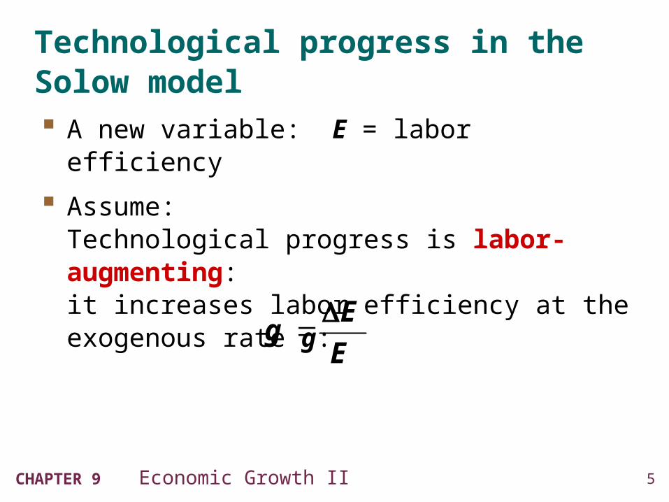
Technological progress in the Solow model A new variable: E = labor efficiency
Assume: Technological progress is labor-augmenting: it increases labor efficiency at the exogenous rate g:
Eg
E
6CHAPTER 9 Economic Growth II
Technological progress in the Solow model
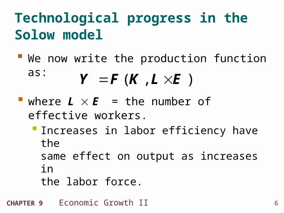
We now write the production function as:
where L E = the number of effective workers. Increases in labor efficiency have the
same effect on output as increases in the labor force.
( , )Y F K L E
7CHAPTER 9 Economic Growth II
Technological progress in the Solow model
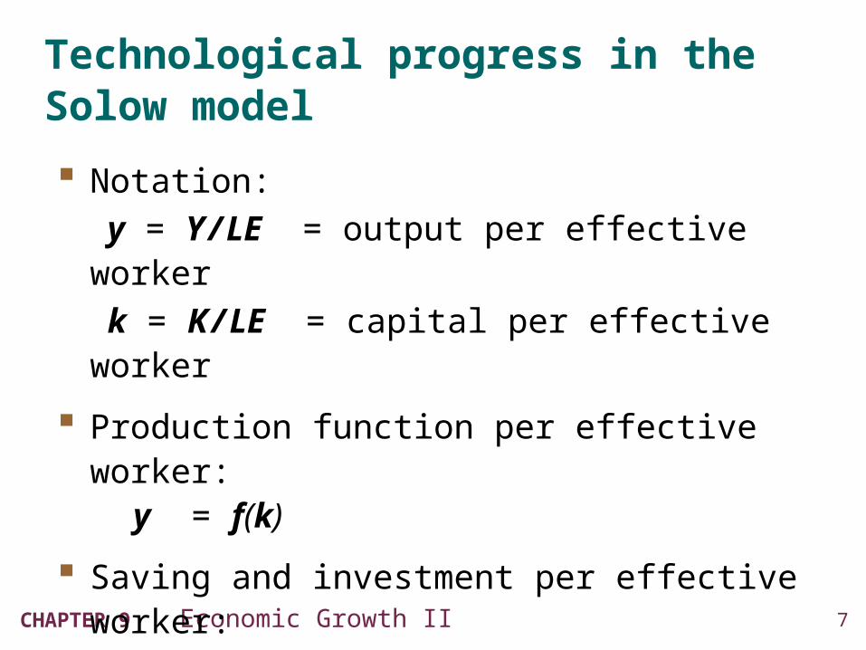
Notation:
y = Y / LE = output per effective worker
k = K / LE = capital per effective worker
Production function per effective worker:y = f(k)
Saving and investment per effective worker:s y = s f(k)
8CHAPTER 9 Economic Growth II
Technological progress in the Solow model
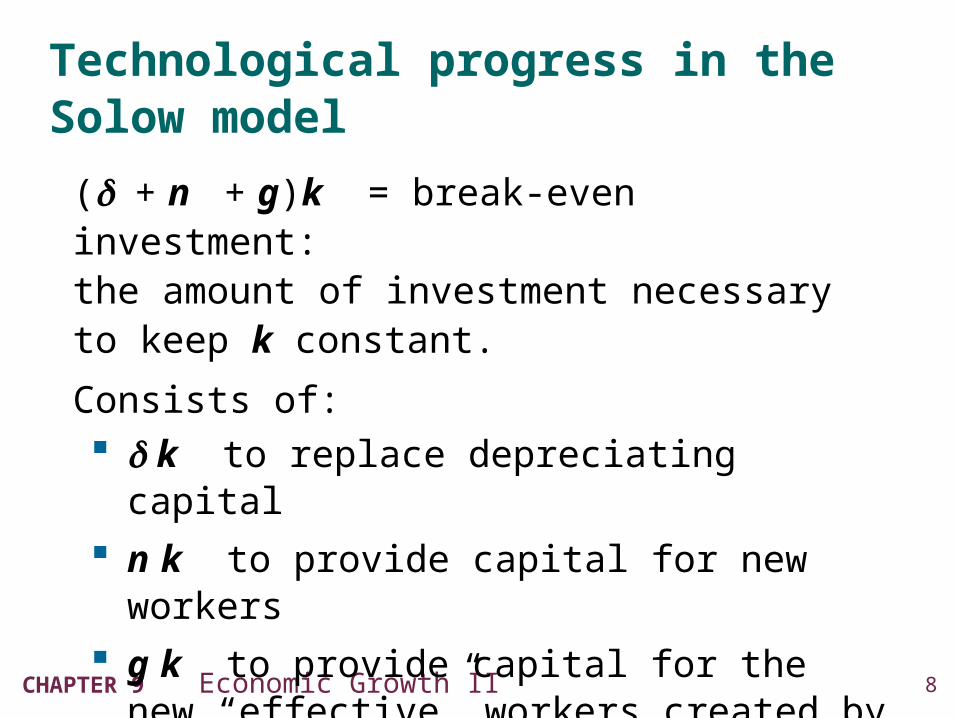
( + n + g)k = break-even investment: the amount of investment necessary to keep k constant.
Consists of: k to replace depreciating capital
n k to provide capital for new workers
g k to provide capital for the new “effective” workers created by technological progress
9CHAPTER 9 Economic Growth II
Technological progress in the Solow model
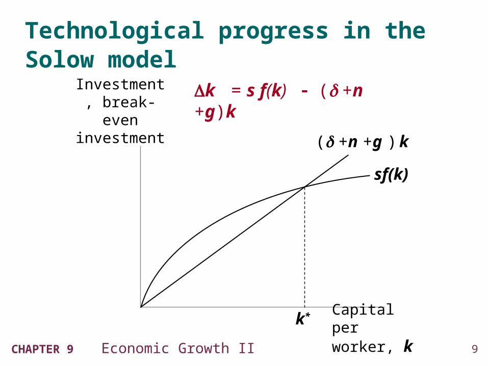
Investment, break-even investment
Capital per worker, k
sf(k)
( +n +g ) k
k*
k = s f(k) ( +n +g)k
10CHAPTER 9 Economic Growth II
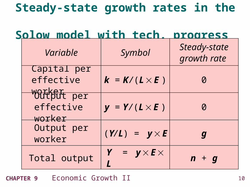
Steady-state growth rates in the Solow model with tech. progress
n + gY = y E L Total output
g(Y/ L) = y E Output per worker
0y = Y / (L E )Output per effective worker
0k = K / (L E )Capital per effective worker
Steady-state growth rate
SymbolVariable
11CHAPTER 9 Economic Growth II
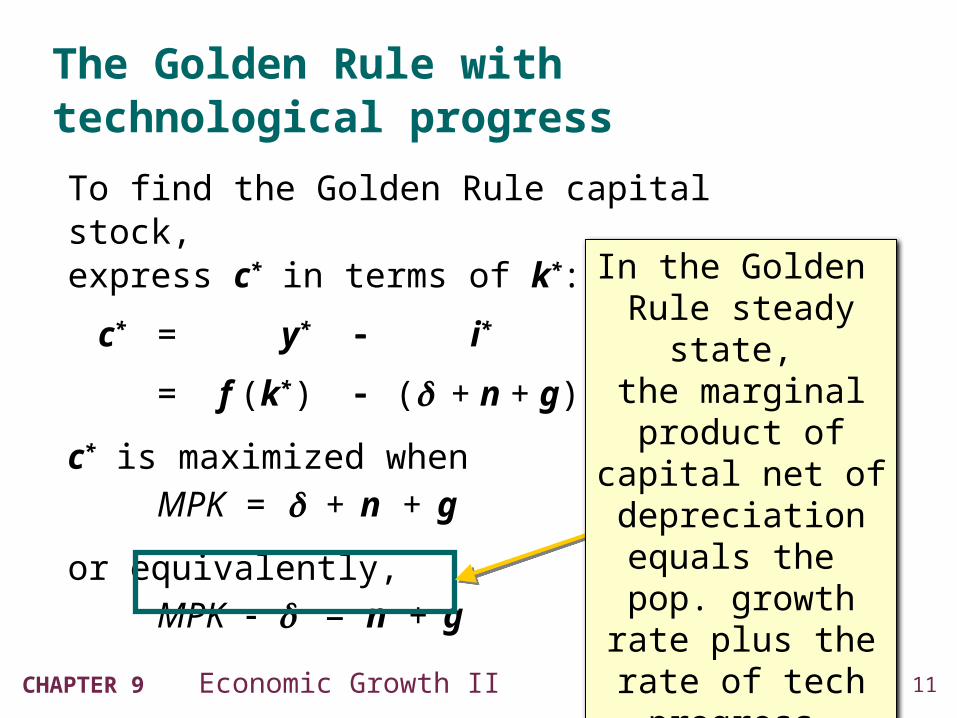
The Golden Rule with technological progress
To find the Golden Rule capital stock, express c* in terms of k*:
c* = y* i*
= f (k* ) ( + n + g) k*
c* is maximized when MPK = + n + g
or equivalently, MPK = n + g
In the Golden Rule steady state,
the marginal product of capital
net of depreciation equals the
pop. growth rate plus the rate of tech progress.
12CHAPTER 9 Economic Growth II
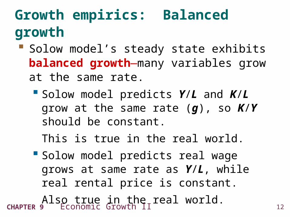
Growth empirics: Balanced growth Solow model’s steady state exhibits
balanced growth—many variables grow at the same rate.
Solow model predicts Y/L and K/L grow at the same rate (g), so K/Y should be constant.
This is true in the real world.
Solow model predicts real wage grows at same rate as Y/L, while real rental price is constant.
Also true in the real world.
13CHAPTER 9 Economic Growth II
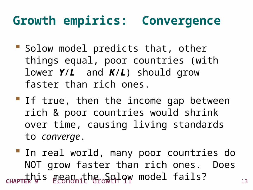
Growth empirics: Convergence
Solow model predicts that, other things equal, poor countries (with lower Y/L and K/L) should grow faster than rich ones.
If true, then the income gap between rich & poor countries would shrink over time, causing living standards to converge.
In real world, many poor countries do NOT grow faster than rich ones. Does this mean the Solow model fails?
14CHAPTER 9 Economic Growth II
Growth empirics: Convergence
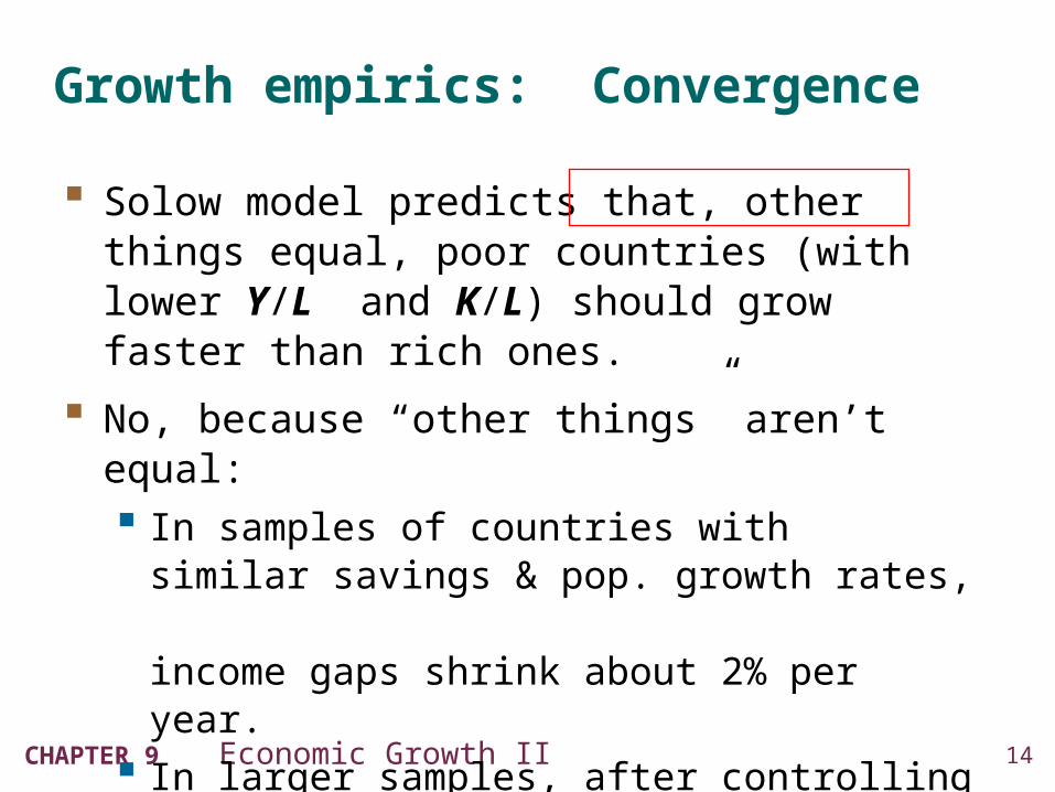
Solow model predicts that, other things equal, poor countries (with lower Y/L and K/L) should grow faster than rich ones.
No, because “other things” aren’t equal: In samples of countries with
similar savings & pop. growth rates, income gaps shrink about 2% per year.
In larger samples, after controlling for differences in saving, pop. growth, and human capital, incomes converge by about 2% per year.
15CHAPTER 9 Economic Growth II
Growth empirics: Convergence
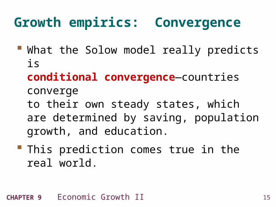
What the Solow model really predicts is conditional convergence—countries converge to their own steady states, which are determined by saving, population growth, and education.
This prediction comes true in the real world.
16CHAPTER 9 Economic Growth II
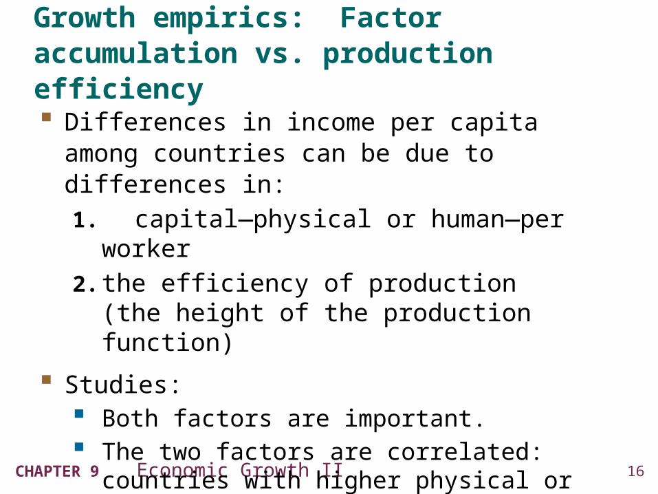
Growth empirics: Factor accumulation vs. production efficiency Differences in income per capita among countries
can be due to differences in:
1. capital—physical or human—per worker
2. the efficiency of production (the height of the production function)
Studies: Both factors are important. The two factors are correlated: countries with
higher physical or human capital per worker also tend to have higher production efficiency.
17CHAPTER 9 Economic Growth II
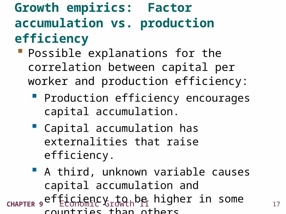
Growth empirics: Factor accumulation vs. production efficiency Possible explanations for the correlation
between capital per worker and production efficiency:
Production efficiency encourages capital accumulation.
Capital accumulation has externalities that raise efficiency.
A third, unknown variable causes capital accumulation and efficiency to be higher in some countries than others.
18CHAPTER 9 Economic Growth II
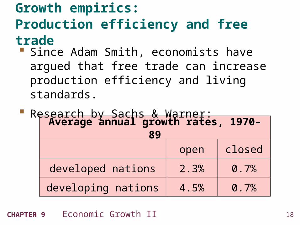
Average annual growth rates, 1970–89
closedopen
Growth empirics: Production efficiency and free trade Since Adam Smith, economists have argued that
free trade can increase production efficiency and living standards.
Research by Sachs & Warner:
0.7%4.5%developing nations
0.7%2.3%developed nations
19CHAPTER 9 Economic Growth II
Growth empirics: Production efficiency and free trade
To determine causation, Frankel and Romer exploit geographic differences among countries: Some nations trade less because they are farther
from other nations, or landlocked. Such geographical differences are correlated with
trade but not with other determinants of income. Hence, they can be used to isolate the impact of
trade on income.
Findings: increasing trade/GDP by 2% causes GDP per capita to rise 1%, other things equal.
20CHAPTER 9 Economic Growth II
Policy issues
Are we saving enough? Too much?
What policies might change the saving rate?
How should we allocate our investment between privately owned physical capital, public infrastructure, and human capital?
How do a country’s institutions affect production efficiency and capital accumulation?
What policies might encourage faster technological progress?
21CHAPTER 9 Economic Growth II
Policy issues: Evaluating the rate of saving Use the Golden Rule to determine whether
the U.S. saving rate and capital stock are too high, too low, or about right.
If (MPK ) > (n + g ), U.S. economy is below the Golden Rule steady state and should increase s.
If (MPK ) < (n + g ), U.S. economy is above the Golden Rule steady state and should reduce s.
22CHAPTER 9 Economic Growth II
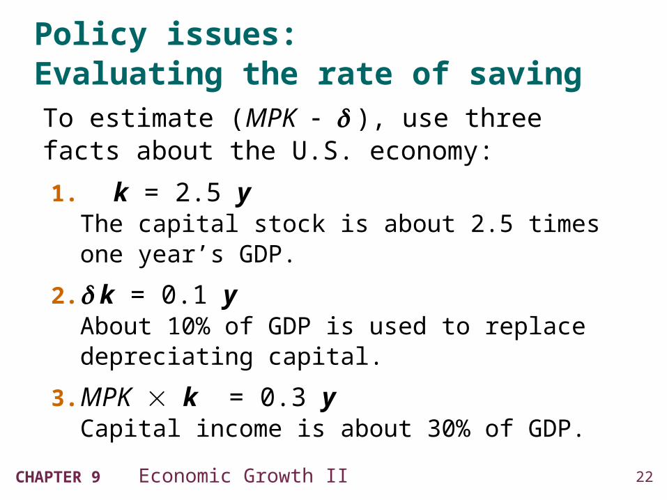
Policy issues: Evaluating the rate of savingTo estimate (MPK ), use three facts about the U.S. economy:
1. k = 2.5 yThe capital stock is about 2.5 times one year’s GDP.
2. k = 0.1 yAbout 10% of GDP is used to replace depreciating capital.
3. MPK k = 0.3 yCapital income is about 30% of GDP.
23CHAPTER 9 Economic Growth II
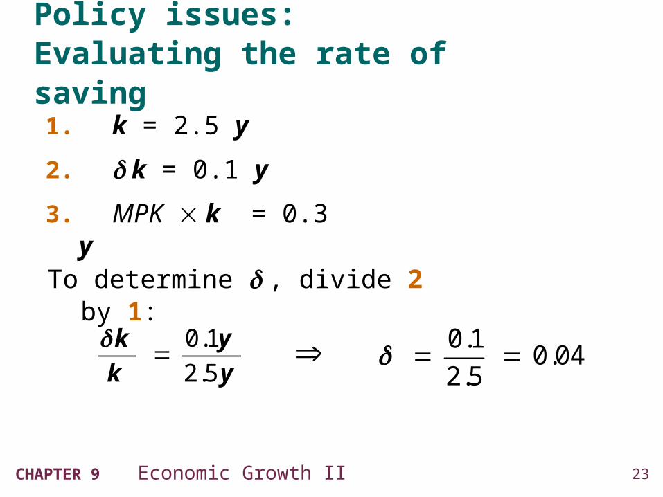
Policy issues: Evaluating the rate of saving1. k = 2.5 y
2. k = 0.1 y
3. MPK k = 0.3 y
0.1
2.5
k yk y
0.1
0.042.5
To determine , divide 2 by 1:
24CHAPTER 9 Economic Growth II
Policy issues: Evaluating the rate of saving
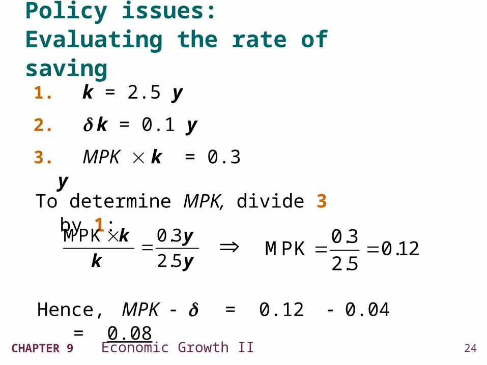
MPK 0.3
2.5
k yk y
0.3
MPK 0.122.5
To determine MPK, divide 3 by 1:
Hence, MPK = 0.12 0.04 = 0.08
1. k = 2.5 y
2. k = 0.1 y
3. MPK k = 0.3 y
25CHAPTER 9 Economic Growth II
Policy issues: Evaluating the rate of saving
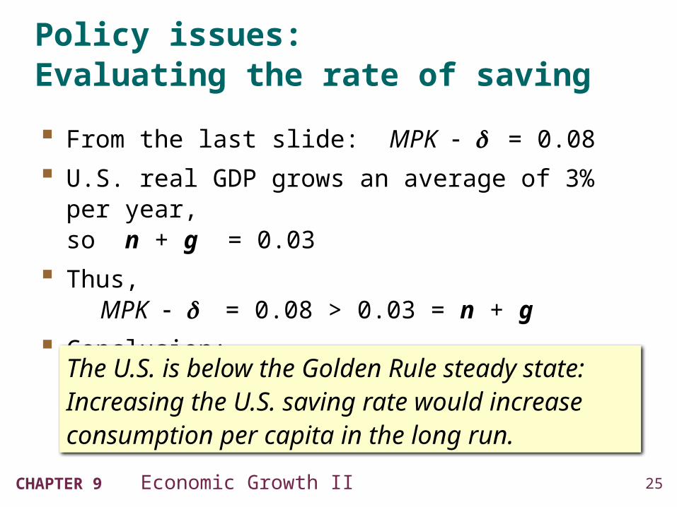
From the last slide: MPK = 0.08
U.S. real GDP grows an average of 3% per year, so n + g = 0.03
Thus, MPK = 0.08 > 0.03 = n + g
Conclusion:
The U.S. is below the Golden Rule steady state: Increasing the U.S. saving rate would increase consumption per capita in the long run.
26CHAPTER 9 Economic Growth II
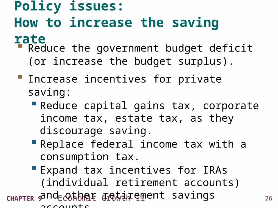
Policy issues: How to increase the saving rate Reduce the government budget deficit
(or increase the budget surplus).
Increase incentives for private saving: Reduce capital gains tax, corporate income tax,
estate tax, as they discourage saving. Replace federal income tax with a consumption
tax. Expand tax incentives for IRAs (individual
retirement accounts) and other retirement savings accounts.
27CHAPTER 9 Economic Growth II
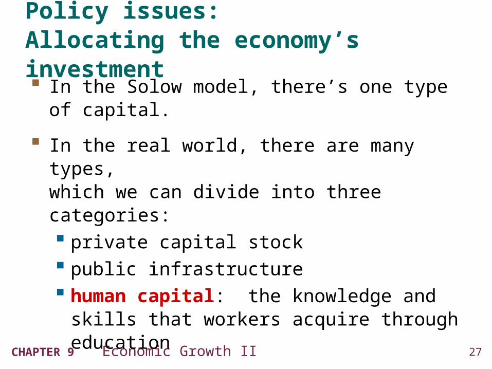
Policy issues: Allocating the economy’s investment In the Solow model, there’s one type of capital.
In the real world, there are many types,which we can divide into three categories: private capital stock public infrastructure human capital: the knowledge and skills that
workers acquire through education
How should we allocate investment among these types?
28CHAPTER 9 Economic Growth II
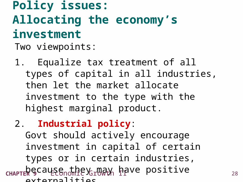
Policy issues: Allocating the economy’s investmentTwo viewpoints:
1. Equalize tax treatment of all types of capital in all industries, then let the market allocate investment to the type with the highest marginal product.
2. Industrial policy: Govt should actively encourage investment in capital of certain types or in certain industries, because they may have positive externalities that private investors don’t consider.
29CHAPTER 9 Economic Growth II
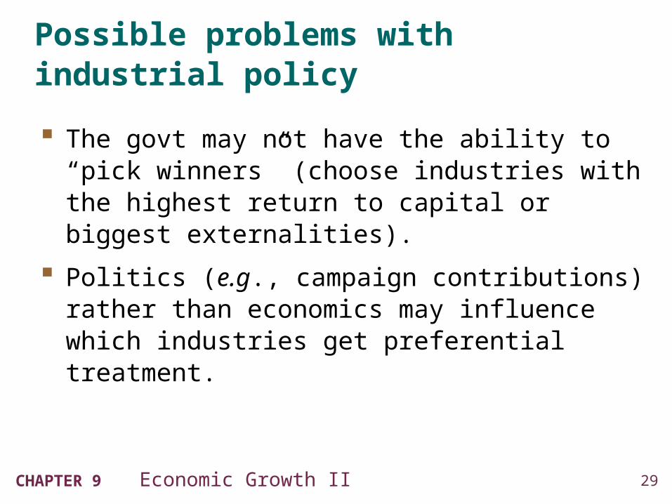
Possible problems with industrial policy
The govt may not have the ability to “pick winners” (choose industries with the highest return to capital or biggest externalities).
Politics (e.g., campaign contributions) rather than economics may influence which industries get preferential treatment.

30CHAPTER 9 Economic Growth II
Policy issues: Establishing the right institutions
Creating the right institutions is important for ensuring that resources are allocated to their best use. Examples:
Legal institutions, to protect property rights.
Capital markets, to help financial capital flow to the best investment projects.
A corruption-free government, to promote competition, enforce contracts, etc.
31CHAPTER 9 Economic Growth II
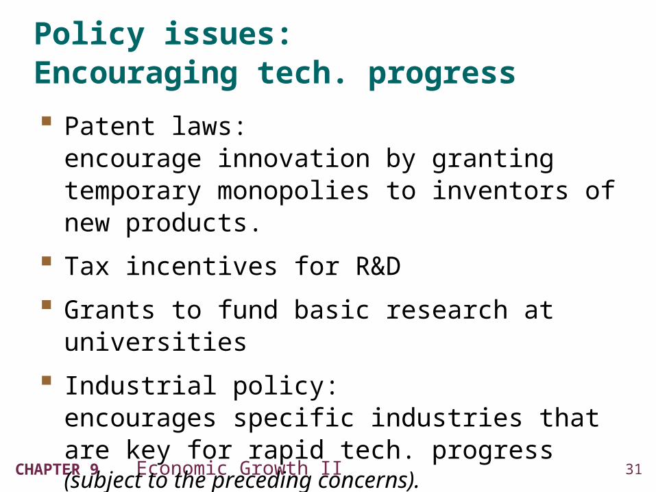
Policy issues: Encouraging tech. progress
Patent laws:encourage innovation by granting temporary monopolies to inventors of new products.
Tax incentives for R&D
Grants to fund basic research at universities
Industrial policy: encourages specific industries that are key for rapid tech. progress (subject to the preceding concerns).
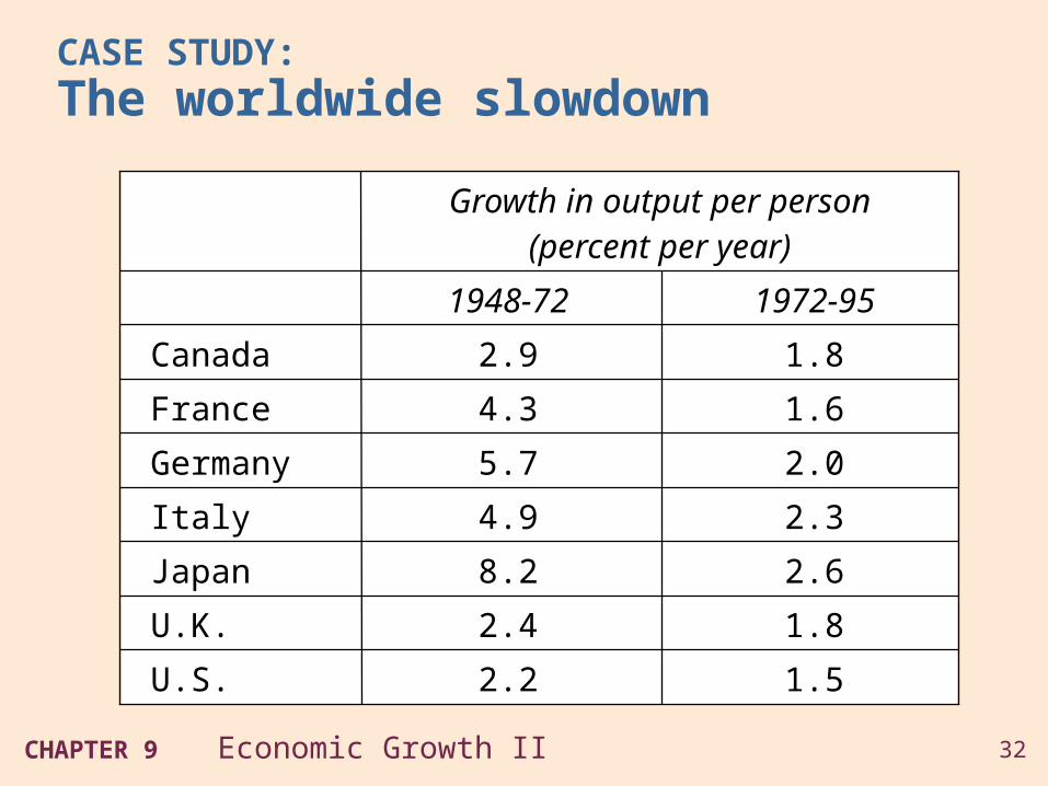
CASE STUDY: The worldwide slowdown
1.5
1.8
2.6
2.3
2.0
1.6
1.8
2.2
2.4
8.2
4.9
5.7
4.3
2.9
1972-951948-72
U.S.
U.K.
Japan
Italy
Germany
France
Canada
Growth in output per person(percent per year)
33CHAPTER 9 Economic Growth II
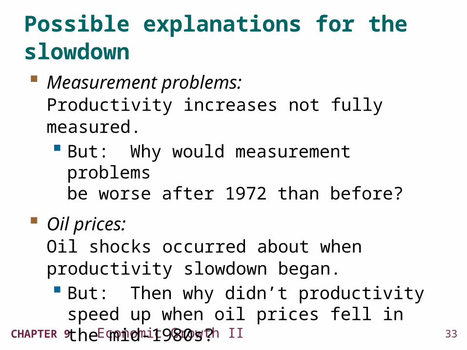
Possible explanations for the slowdown Measurement problems:
Productivity increases not fully measured. But: Why would measurement problems
be worse after 1972 than before?
Oil prices:Oil shocks occurred about when productivity slowdown began. But: Then why didn’t productivity speed up
when oil prices fell in the mid-1980s?
34CHAPTER 9 Economic Growth II
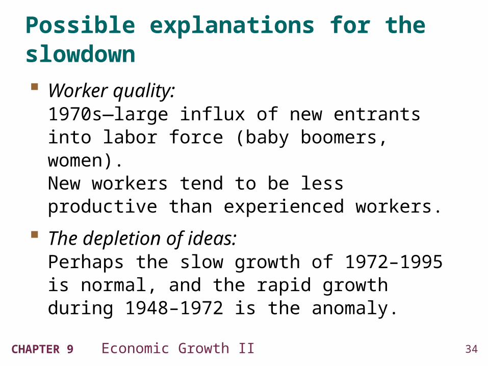
Possible explanations for the slowdown Worker quality:
1970s—large influx of new entrants into labor force (baby boomers, women).New workers tend to be less productive than experienced workers.
The depletion of ideas:Perhaps the slow growth of 1972–1995 is normal, and the rapid growth during 1948–1972 is the anomaly.

35CHAPTER 9 Economic Growth II
Which of these suspects is the culprit?
All of them are plausible, but it’s difficult to prove
that any one of them is guilty.
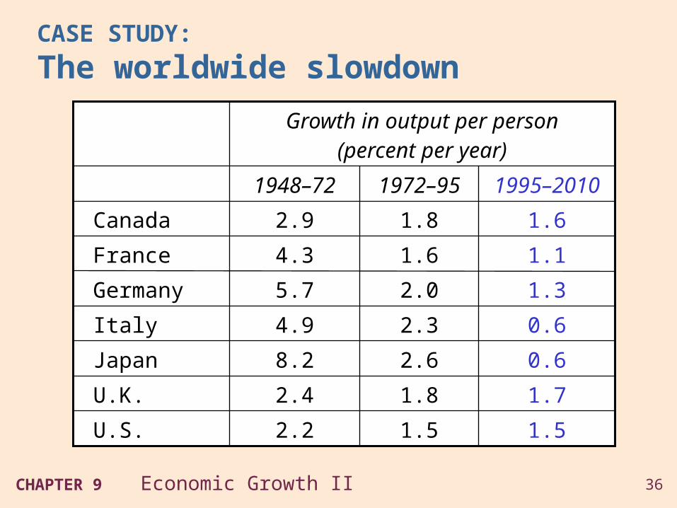
CASE STUDY:
The worldwide slowdown
1.5
1.7
0.6
0.6
1.3
1.1
1.6
1.5
1.8
2.6
2.3
2.0
1.6
1.8
2.2
2.4
8.2
4.9
5.7
4.3
2.9
1995–20101972–951948–72
U.S.
U.K.
Japan
Italy
Germany
France
Canada
Growth in output per person(percent per year)
37CHAPTER 9 Economic Growth II
CASE STUDY:
The worldwide slowdown
The computer revolution and Internet began to affect aggregate productivity in mid-1990s continuing into the mid 2000s.
This period was then offset by the financial crisis and deep recession of 2008–2009.
38CHAPTER 9 Economic Growth II
Endogenous growth theory
Solow model: sustained growth in living standards is due to
tech progress. the rate of tech progress is exogenous.
Endogenous growth theory: a set of models in which the growth rate of
productivity and living standards is endogenous.
39CHAPTER 9 Economic Growth II
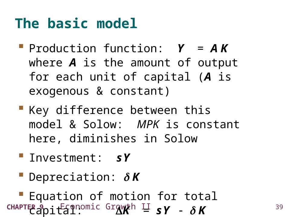
The basic model
Production function: Y = A Kwhere A is the amount of output for each unit of capital (A is exogenous & constant)
Key difference between this model & Solow: MPK is constant here, diminishes in Solow
Investment: s Y
Depreciation: K
Equation of motion for total capital: K = s Y K
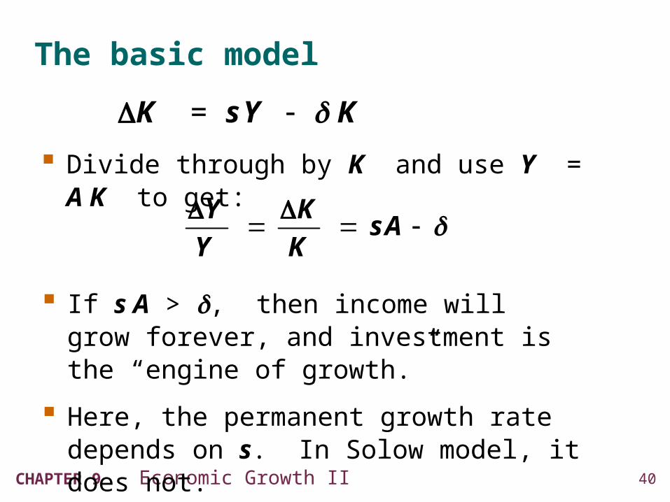
40CHAPTER 9 Economic Growth II
The basic model
K = s Y K
Y KsA
Y K
If s A > , then income will grow forever, and investment is the “engine of growth.”
Here, the permanent growth rate depends on s. In Solow model, it does not.
Divide through by K and use Y = A K to get:
41CHAPTER 9 Economic Growth II
Does capital have diminishing returns or not?
Depends on definition of capital.
If capital is narrowly defined (only plant & equipment), then yes.
Advocates of endogenous growth theory argue that knowledge is a type of capital.
If so, then constant returns to capital is more plausible, and this model may be a good description of economic growth.
42CHAPTER 9 Economic Growth II
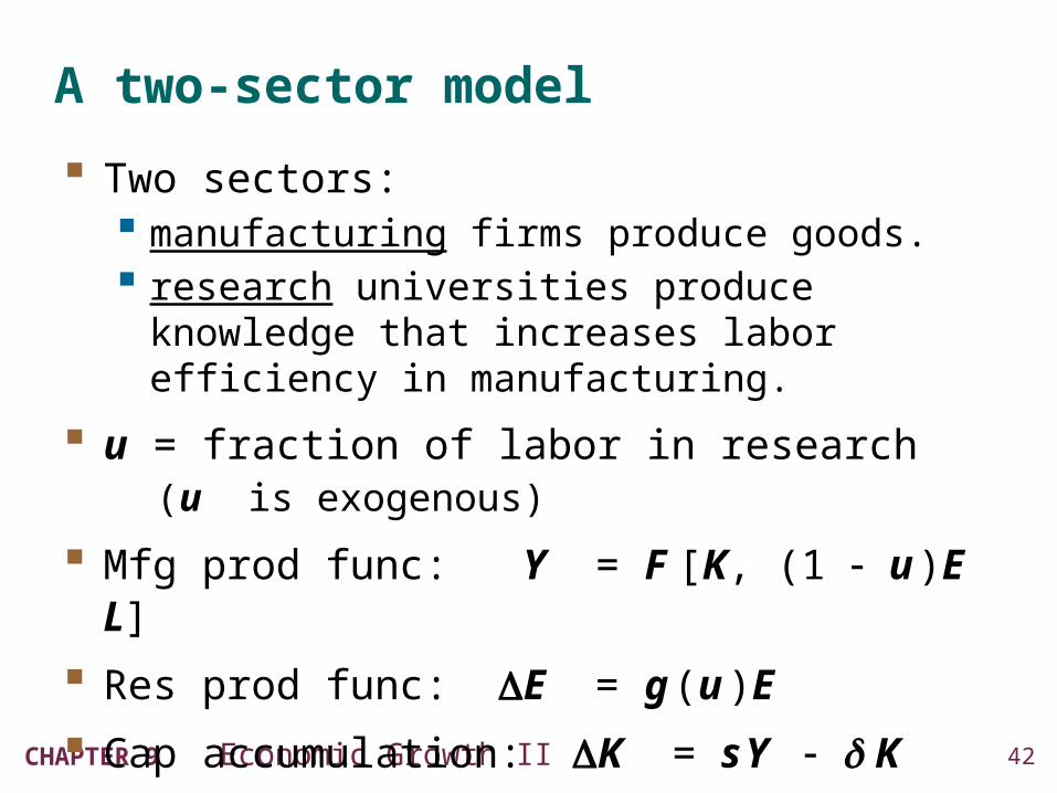
A two-sector model
Two sectors: manufacturing firms produce goods. research universities produce knowledge that
increases labor efficiency in manufacturing.
u = fraction of labor in research (u is exogenous)
Mfg prod func: Y = F [K, (1 u )E L]
Res prod func: E = g (u )E
Cap accumulation: K = s Y K
43CHAPTER 9 Economic Growth II
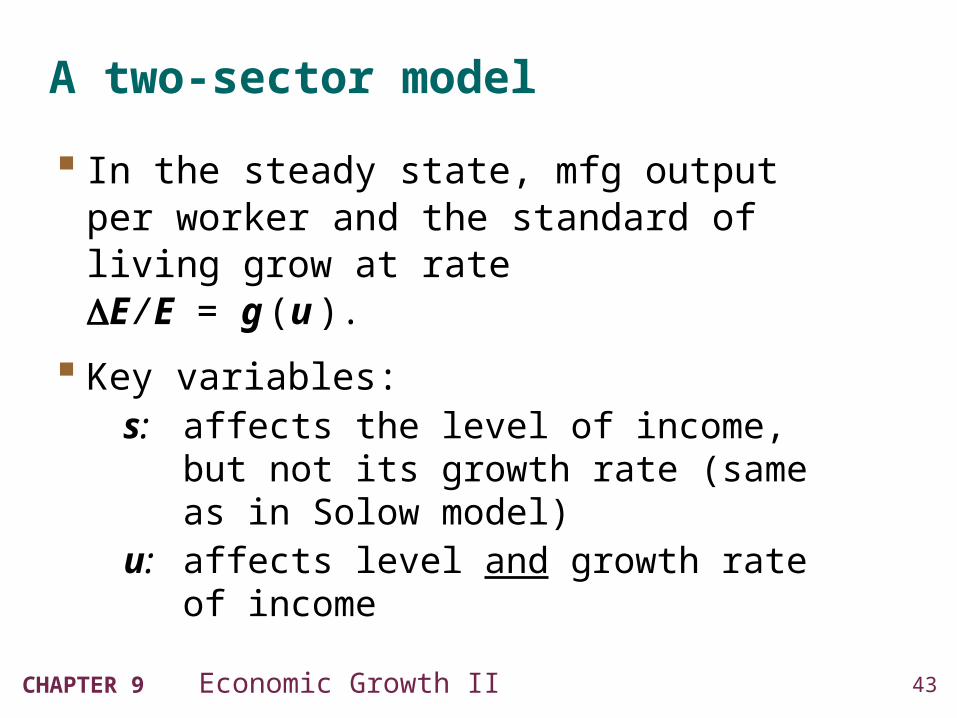
A two-sector model
In the steady state, mfg output per worker and the standard of living grow at rate E / E = g (u ).
Key variables:s: affects the level of income, but not its
growth rate (same as in Solow model)u: affects level and growth rate of income

DISCUSSION QUESTION
The merits of raising u
Question:
Would an increase in u (i.e. devoting more labor to research) be unambiguously good for the economy?
Why or why not?
44
45CHAPTER 9 Economic Growth II
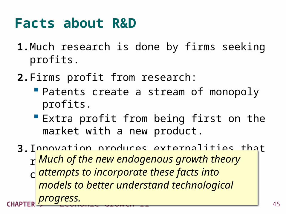
Facts about R&D
1. Much research is done by firms seeking profits.
2. Firms profit from research: Patents create a stream of monopoly profits. Extra profit from being first on the market with a
new product.
3. Innovation produces externalities that reduce the cost of subsequent innovation.
Much of the new endogenous growth theory attempts to incorporate these facts into models to better understand technological progress.
46CHAPTER 9 Economic Growth II
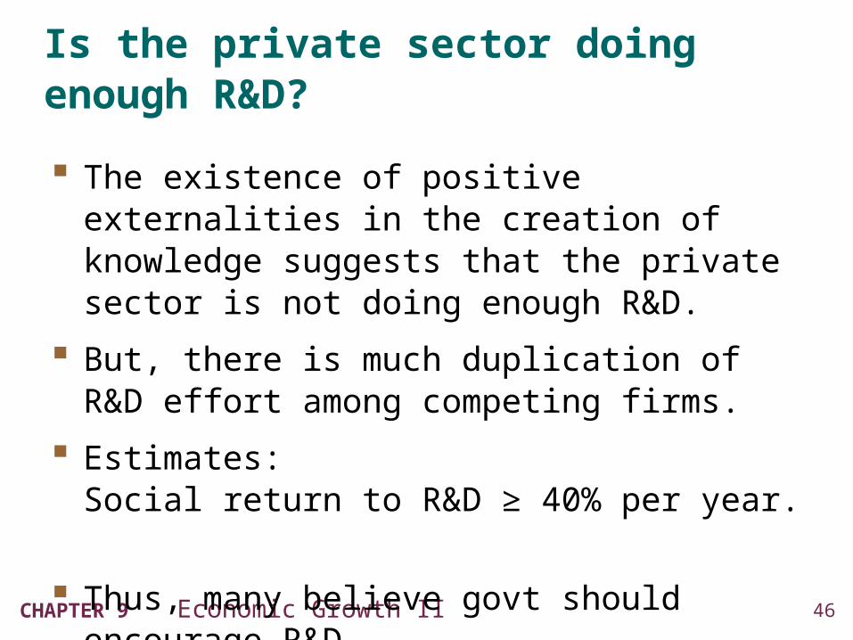
Is the private sector doing enough R&D?
The existence of positive externalities in the creation of knowledge suggests that the private sector is not doing enough R&D.
But, there is much duplication of R&D effort among competing firms.
Estimates: Social return to R&D ≥ 40% per year.
Thus, many believe govt should encourage R&D.

47CHAPTER 9 Economic Growth II
Economic growth as “creative destruction”
Schumpeter (1942) coined term “creative destruction” to describe displacements resulting from technological progress: the introduction of a new product is good for
consumers but often bad for incumbent producers, who may be forced out of the market.
Examples: Luddites (1811–12) destroyed machines that
displaced skilled knitting workers in England. Walmart displaces many mom-and-pop stores.
C H A P T E R S U M M A R Y
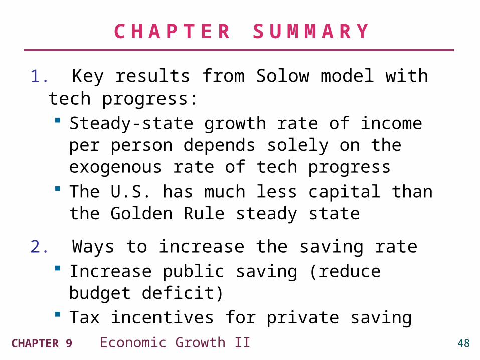
1. Key results from Solow model with tech progress: Steady-state growth rate of income per person
depends solely on the exogenous rate of tech progress
The U.S. has much less capital than the Golden Rule steady state
2. Ways to increase the saving rate Increase public saving (reduce budget deficit) Tax incentives for private saving
48
C H A P T E R S U M M A R Y
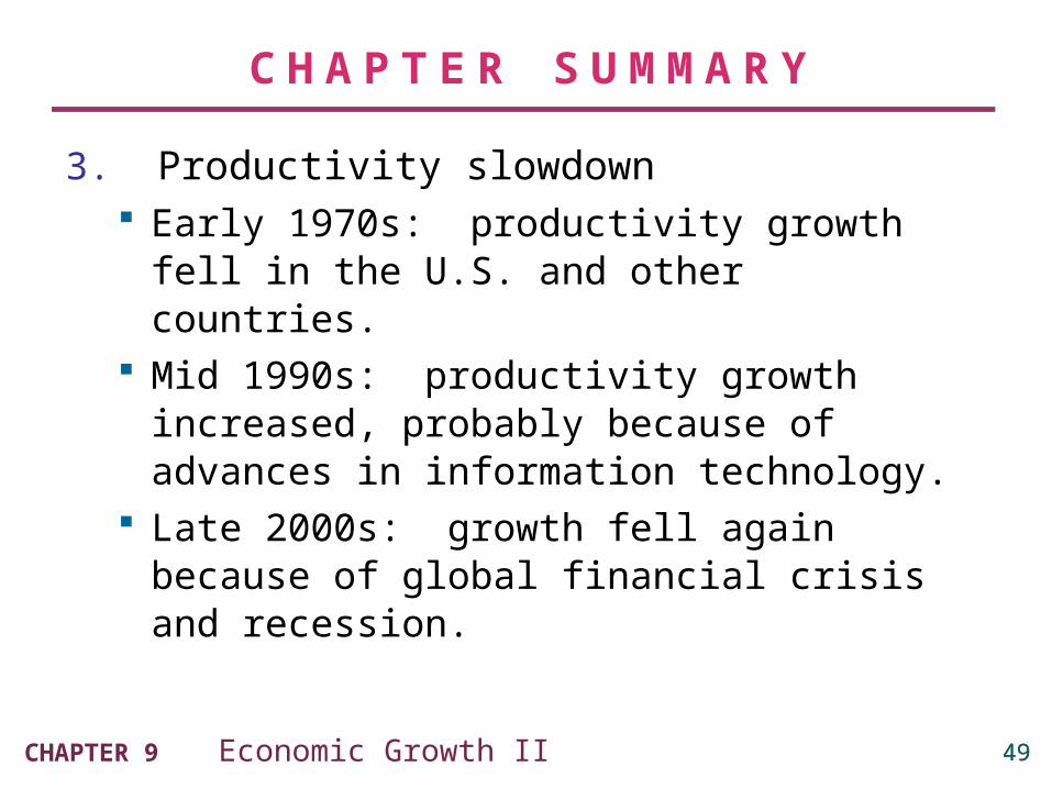
3. Productivity slowdown Early 1970s: productivity growth fell in the U.S.
and other countries. Mid 1990s: productivity growth increased,
probably because of advances in information technology.
Late 2000s: growth fell again because of global financial crisis and recession.
49
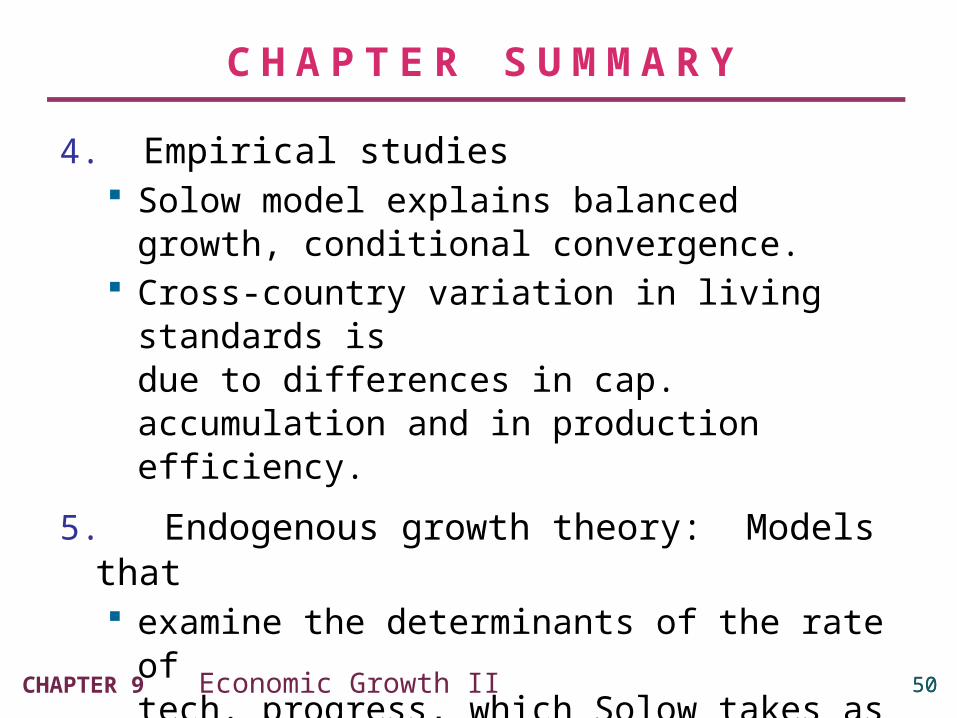
C H A P T E R S U M M A R Y
4. Empirical studies Solow model explains balanced growth,
conditional convergence. Cross-country variation in living standards is
due to differences in cap. accumulation and in production efficiency.
5. Endogenous growth theory: Models that examine the determinants of the rate of
tech. progress, which Solow takes as given. explain decisions that determine the creation of
knowledge through R&D.
50


![[PPT] Mankiw 6e PowerPoints€¦ · Web viewTitle Mankiw 6e PowerPoints Author Ron Cronovich Last modified by usuario Created Date 4/29/2006 12:50:43 AM Document presentation format](https://img.pdfslide.us/doc/110x75/5eba8f71dde7f6377925430c/ppt-mankiw-6e-powerpoints-web-view-title-mankiw-6e-powerpoints-author-ron-cronovich.jpg)


![[PPT]Mankiw 6e PowerPoints · Web viewTitle Mankiw 6e PowerPoints Author Ron Cronovich Last modified by usuario Created Date 4/29/2006 12:50:43 AM Document presentation format Presentación](https://img.pdfslide.us/doc/110x75/5bd3f63109d3f29b578b7917/pptmankiw-6e-powerpoints-web-viewtitle-mankiw-6e-powerpoints-author-ron-cronovich.jpg)