Macroeconomic Uncertainty and Expected Stock Returns

Turan G. Bali∗

Georgetown UniversityStephen J. Brown†

New York UniversityYi Tang‡

Fordham University

Abstract

This paper introduces a broad index of macroeconomic uncertainty based on the ex-antemeasures of cross-sectional dispersion in economic forecasts by the Survey of ProfessionalForecasters. We estimate individual stock exposures to a newly proposed measure of eco-nomic uncertainty index and find that the resulting uncertainty beta predicts a significantproportion of the cross-sectional dispersion in stock returns. After controlling for a largeset of stock characteristics and risk factors, we find the predicted negative relation betweenuncertainty beta and future stock returns remains economically and statistically significant.The significantly negative uncertainty premium is robust to alternative measures of uncer-tainty index and distinct from the negative market volatility risk premium identified byearlier studies.

This draft: December 2014

JEL classification: G11, G12, C13, E20, E30.

Keywords: Macroeconomic uncertainty, dispersion in economic forecasts, cross-section of stock returns, re-turn predictability.

∗Robert S. Parker Professor of Business Administration, McDonough School of Business, Georgetown University, Washington, D.C.20057. Email: tgb27@georgetown.edu. Phone: (202) 687-5388. Fax: (202) 687-4031.

†David S. Loeb Professor of Finance, Stern School of Business, New York University, New York, NY 10012, and Professorial Fellow,University of Melbourne, Email: sbrown@stern.nyu.edu.

‡Associate Professor of Finance, Schools of Business, Fordham University, 1790 Broadway, New York, NY 10019. Email:ytang@fordham.edu. Phone: (646) 312-8292. Fax: (646) 312-8295.

An earlier draft of this paper was circulated under the title “Cross-Sectional Dispersion in Economic Forecasts and Expected Stock Re-turns.” We thank Jennie Bai, Geert Bekaert, Nick Bloom, John Campbell, and Sydney Ludvigson for their extremely helpful comments andsuggestions. We also benefited from discussions with Senay Agca, Reena Aggarwal, Oya Altinkilic, Bill Baber, Audra Boone, Yong Chen,Jess Cornaggia, Michael Gordy, Shane Johnson, Gergana Jostova, Hagen Kim, James Kolari, Yan Liu, Arvind Mahajan, Paul Peyser, LeePinkowitz, Christo Pirinsky, Marco Rossi, Kevin Sheppard, Wei Tang, Ashley Wang, Sumudu Watugala, Rohan Williamson, Kamil Yilmaz,and seminar participants at the Federal Reserve Board, George Washington University, Georgetown University, Koc University, the Office ofFinancial Research at the U.S. Department of the Treasury, and Texas A&M University. All errors remain our responsibility.

1. Introduction

Merton’s (1973) seminal paper indicates that, in a multi-period economy, investors have incentive to

hedge against future stochastic shifts in consumption and investment opportunity sets. This implies that

state variables that are correlated with changes in consumption and investment opportunities are priced

in capital markets such that an asset’s covariance with these state variables is related to its expected

returns.

Macroeconomic variables are widely accepted candidates for these systematic risk factors because

innovations in economic indicators can generate global impacts on stock fundamentals, such as cash

flows, risk-adjusted discount factors, and investment opportunities. There are several channels by which

macroeconomic fundamentals such as output growth, inflation, and unemployment have significant

impacts on expected returns. To the extent that investors pursue opportunities arising from changing

economic circumstances, we would expect that returns from investment in risky assets are influenced

by the extent to which investors vary their exposure to leading economic indicators.

According to the intertemporal capital asset pricing model (ICAPM) of Merton (1973), investors are

concerned not only with the terminal wealth that their portfolio produces, but also with the investment

and consumption opportunities that they will have in the future. Hence, when choosing a portfolio at

time t, ICAPM investors consider how their wealth at time t +1 might vary with future state variables.

This implies that like CAPM investors, ICAPM investors prefer high expected return and low return

variance, but they are also concerned with the covariances of portfolio returns with state variables that

affect future investment opportunities. Bloom, Bond, and Reenen (2007), Bloom (2009), Chen (2010),

Allen, Bali, and Tang (2012), Bloom, Floetotto, Jaimovich, Saporta-Eksten, and Terry (2012), and

Stock and Watson (2012) provide theoretical and empirical support for the idea that time variation in

the conditional volatility of macroeconomic shocks is linked to real economic activity. Thus, economic

uncertainty is a relevant state variable affecting future consumption and investment decisions.

Motivated by the aforementioned studies, we examine the role of macroeconomic uncertainty in

the cross-sectional pricing of individual stocks. We argue that disagreement over changes in macroe-

conomic fundamentals can be considered a source of macroeconomic uncertainty. We quantify this

1

uncertainty with ex-ante measures of cross-sectional dispersion in economic forecasts from the Sur-

vey of Professional Forecasters. These uncertainty measures provided by the Federal Reserve Bank of

Philadelphia determine the degree of disagreement between the expectations of professional forecast-

ers. In our empirical analysis, we use seven different measures of cross-sectional dispersion in quarterly

forecasts for output, inflation, and unemployment as alternative proxies for economic uncertainty.

We quantify an unexpected change in economic predictions of professional forecasters by esti-

mating an autoregressive process for each dispersion measure. The standardized residuals from the

autoregressive model remove the predictable component of the dispersion measures and can be viewed

as a measure of uncertainty shock. We estimate individual stock exposure to the standardized residuals

and find that the resulting uncertainty betas from all seven measures of uncertainty shock predict a

significant proportion of the cross-sectional dispersion in stock returns.

In addition to individual measures of disagreement over macroeconomic fundamentals, we intro-

duce two broad indices of economic uncertainty based on the average and the first principal component

of the standardized residuals for the seven dispersion measures. These economic uncertainty indices

are generated using the past information only, so that there is no look-ahead bias in our empirical anal-

yses. Moreover, these uncertainty indices are formed based on the ex-ante predictions of professional

forecasters so that we provide out-of-sample performance of the ex-ante measure of the uncertainty

beta in predicting the cross-sectional variation in future stock returns.

First, we estimate time-varying uncertainty betas using 20-quarter (and 60-month) rolling regres-

sions of excess returns on the newly proposed economic uncertainty index for each stock trading at

the NYSE, Amex, and Nasdaq. Then, we examine the performance of these quarterly (and monthly)

uncertainty betas in predicting the cross-sectional dispersion in future stock returns. Specifically, we

sort stocks into decile portfolios by their uncertainty beta during the previous quarter (or month) and

examine the monthly returns on the resulting portfolios from October 1973 to December 2012. Stocks

in the lowest uncertainty beta decile generate about 8% more annual returns compared to stocks in the

highest uncertainty beta decile. After controlling for the well-known market, size, book-to-market, and

momentum factors of Fama and French (1993) and Carhart (1997), we find the difference between the

2

returns on the portfolios with the highest and lowest uncertainty beta (4-factor alpha) remains negative

and highly significant.

The significantly negative uncertainty premium is consistent with the intertemporal capital asset

pricing models of Merton (1973) and Campbell (1993, 1996). An increase in economic uncertainty

reduces future investment and consumption opportunities. To hedge against unfavorable shifts in in-

vestment opportunity sets, investors prefer to hold stocks that have higher covariance with economic

uncertainty (stocks with higher uncertainty beta). This is because an increase in economic uncertainty

increases the return on high uncertainty beta stocks due to positive intertemporal correlation. Hence,

when economic uncertainty increases, although their optimal consumption and future investment op-

portunities decline, investors compensate for this loss by obtaining a stronger wealth effect through the

increase in the returns of stocks that have a positive correlation with economic uncertainty. Therefore,

through the intertemporal hedging demand, investors prefer to hold stocks with higher uncertainty beta,

and accept lower compensation from these stocks in the form of lower expected returns.

In addition to the rational asset pricing explanation of the negative uncertainty premium, there

exists a behavioral explanation based on differences of opinion and short-sales constraints along the

lines of Miller (1977).1 Suppose that stocks with high uncertainty beta are subject to overpricing

because investor opinions differ about their prospects and they are hard to short. When macroeconomic

uncertainty increases, the range of investor opinions about their prospects broadens. More extreme

optimists end up holding these stocks, and their prices increase. The uncertainty beta can thus be

viewed as an indirect way to measure dispersed opinion and overpricing. This view suggests that these

stocks should have particularly low returns when economic uncertainty is high. Although exploring

Miller’s hypothesis itself is beyond the scope of this paper, we show later in the paper that stocks with

high uncertainty beta have particularly low returns during economic recessions with larger differences

of opinion.

1Miller (1977) hypothesizes that stock prices reflect an upward bias as long as divergence of opinion exists among in-vestors about stock value and pessimistic investors do not hold sufficient short positions because of institutional or behavioralreasons. In Miller’s model, overvaluation of securities is observed because pessimists are restricted to holding zero sharesalthough they prefer holding a negative quantity, and the prices of securities are mainly determined by the beliefs of the mostoptimistic investors. Since divergence of opinion is likely to increase with firm-specific uncertainty, Miller predicts a negativerelation between firm-specific uncertainty and expected stock returns.

3

To ensure that it is the uncertainty beta that is driving documented return differences rather than

well-known stock characteristics or risk factors, we perform bivariate portfolio sorts and re-examine

the raw return and alpha differences. We control for size and book-to-market (Fama and French

1992, 1993), momentum (Jegadeesh and Titman 1993), short-term reversal (Jegadeesh 1990), illiq-

uidity (Amihud 2002), co-skewness (Harvey and Siddique 2000), idiosyncratic volatility (Ang, Ho-

drick, Xing, and Zhang 2006), analyst earnings forecast dispersion (Diether, Malloy, Scherbina 2002),

market volatility beta (Ang et al. 2006 and Campbell et al. 2012), firm age (Shumway 2001), and

leverage (Bhandari 1988). After controlling for this large set of stock return predictors, we find the

negative relation between uncertainty beta and future returns remains highly significant. We also ex-

amine the cross-sectional relation between uncertainty beta and expected returns at the stock-level

using the Fama-MacBeth (1973) regressions. After all variables are controlled for simultaneously, the

cross-sectional regressions provide strong corroborating evidence for an economically and statistically

significant negative relation between the uncertainty beta and future stock returns.

We provide a battery of robustness checks. We investigate whether our results are driven by small,

illiquid, and low-priced stocks, or stocks trading at the Amex and Nasdaq exchanges. We find that neg-

ative uncertainty premium is highly significant in the cross-section of NYSE stocks, S&P 500 stocks,

and the 1,000 and 500 largest and most liquid stocks in the Center for Research in Security Prices

(CRSP) universe. We show that the cross-sectional predictability results are robust across different

time periods, and for both economic recessions and expansions. However, consistent with theoretical

predictions, the uncertainty premium is higher during bad states of the economy. We also examine

the long-term predictive power of uncertainty beta and find that the negative relation between the un-

certainty beta and future stock returns is not just a one-month affair. The economic uncertainty beta

predicts cross-sectional variations in stock returns nine months into the future. Finally, we show that

the negative uncertainty premium is significant when we use the alternative measures of the economic

uncertainty index developed by Jurado, Ludvigson, and Ng (2013). Moreover, this negative uncertainty

premium is distinct from the negative volatility risk premium identified by earlier studies.

The paper is organized as follows. Section 2 describes the data and variables. Section 3 presents

a simple extension of Merton’s (1973) conditional asset pricing model with economic uncertainty.

4

Section 4 provides portfolio-level analyses and stock-level cross-sectional regressions that examine

a comprehensive list of control variables. Section 5 controls for exposure to stock market volatility.

Section 6 investigates whether our main findings remain intact when we use alternative measures of the

economic uncertainty index proposed by other studies. Section 7 concludes the paper.

2. Data and variable definitions

This section first describes the data on cross-sectional dispersion in economic forecasts, and then in-

troduces an index of macroeconomic uncertainty. Finally, we provide the definitions of the stock-level

predictive variables used in cross-sectional return predictability.

2.1. Cross-sectional dispersion in economic forecasts

The Federal Reserve Bank of Philadelphia releases measures of cross-sectional dispersion in economic

forecasts from the Survey of Professional Forecasters, calculating the degree of disagreement between

the expectations of different forecasters.2 In our empirical analyses, we use the cross-sectional disper-

sion in quarterly forecasts for the U.S. real gross domestic product (GDP) growth, real GDP (RGDP)

level, nominal GDP (NGDP) level, NGDP growth, GDP price index level, GDP price index growth

(inflation rate forecast), and unemployment rate. These dispersion measures are model-independent,

nonparametric measures of economic uncertainty obtained from disagreements among professional

forecasters.3 The cross-sectional dispersion measures are defined as the percent difference between the

75th and 25th percentiles (the interquartile range) of the projections for quarterly growth or levels:

Dispersion Measure(Growth) = 100× log(75th Growth/25th Growth), (1)

Dispersion Measure(Level) = 100× log(75th Level/25th Level). (2)

2The Survey of Professional Forecasters is the oldest quarterly survey of macroeconomic forecasts in the United States.The survey began in 1968 and was conducted by the American Statistical Association and the National Bureau of EconomicResearch. The Federal Reserve Bank of Philadelphia took over the survey in 1990.

3The Federal Reserve Bank of Philadelphia provides a partial list of the forecasters who participated in the survey. Pro-fessional forecasters are generally academics at research institutions and economists at major investment banks, consultingfirms, and central banks in the United States and abroad. The number of professional forecasters who participate in thesurvey changes over time. Figure A1 of the online appendix presents the number of forecasts for the current quarter’s realGDP growth over the sample period 1968:Q4−2012:Q4. The number of forecasts for the other six macro variables is almostidentical for the period 1968−2012.

5

Panel A in Table A1 of the online appendix presents the descriptive statistics of the quarterly cross-

sectional dispersion measures for the sample period 1968:Q4−2012:Q4. The volatility and max-min

differences of the dispersion measures are quite high compared to their means, implying significant

time-series variation in the economic uncertainty measures. Panel B of Table A1 shows that the

cross-sectional dispersion measures are generally highly correlated with each other (in the range of

0.74−0.95), and reflect common sources of ambiguity about the state of the aggregate economy. On

the other hand, some of the correlations reported in Panel B of Table A1 are lower, in the range of

0.34−0.59, implying that each dispersion measure has the potential to capture different aspects of un-

certainty and disagreement over financial and macroeconomic fundamentals.

Figure A2 of the online appendix displays the quarterly time-series plots of the cross-sectional

dispersion measures for the sample period 1968:Q4−2012:Q4. The visual depiction of the dispersion

measures in Figure A2 indicates that these economic uncertainty measures closely follow large falls and

rises in financial and economic activity. Specifically, economic uncertainty is higher during economic

and financial market downturns. Similarly, uncertainty is higher during periods corresponding to high

levels of default and credit risk as well as stock market crashes. Lastly, uncertainty about inflation,

uncertainty about output growth, and uncertainty about unemployment are generally higher during bad

states of the economy corresponding to periods of high unemployment, low output growth, and low

economic activity.4

2.2. Economic uncertainty index

In this section, we introduce a broad index of economic uncertainty based on innovations in the cross-

sectional dispersion in economic forecasts. As presented in the last column of Table A1, Panel A, the

cross-sectional dispersion measures are highly persistent. The first-order autocorrelation coefficients

are in the range of 0.28 and 0.73, but they are significantly below one. Therefore, unexpected change

(or shock) to economic predictions of professional forecasters is not defined with a simple change in

4Specifically, the spikes in Figure A2 closely follow major economic and financial crisis such as the 1973 oil crisis, the1973−1974 stock market crash, the 1979−1982 high interest rate period, the 1980s Latin American debt crisis, the 1989-1991savings and loan crisis in the United States, the recession of the early 1990s, the 1997−1998 Asian and Russian financialcrises, the recession of the early 2000s, and the recent global financial crisis (2007-2009).

6

dispersion measures. Instead, we estimate the following autoregressive of order one, AR(1), process

for each dispersion measure:

Zt = ω0 +ω1Zt−1 + εt , (3)

where Zt is one of the seven measures of cross-sectional dispersion in economic forecasts; the real GDP

growth and level, the nominal GDP growth and level, the GDP price index growth and level (proxying

for the inflation rate), and the unemployment rate.

For each dispersion measure and for each quarter, we estimate equation (3) using the quarterly

rolling regressions over a 20-quarter fixed window period. Then, we generate the standardized resid-

uals from the AR(1) model for each dispersion measure. The economic uncertainty index (UNCAV G)

is defined as the average of the standardized residuals for the seven dispersion measures, and it can be

viewed as a broad measure of the shock to dispersion in the forecasts of output, inflation and unem-

ployment.

The first-order autocorrelation coefficients of the innovations in dispersion measures are in the

range of −0.04 and −0.18, much lower than the serial correlations in raw measures of dispersion

(in absolute magnitude). This result indicates that the standardized residuals from the AR(1) model

successfully remove the predictable component of the dispersion measures so that the economic uncer-

tainty index (UNCAV G) is a measure of uncertainty shock capturing different aspects of disagreement

over macroeconomic fundamentals and also reflecting unexpected news or surprise about the state of

the aggregate economy.

It is important to note that the economic uncertainty index is generated for each quarter using the

past information only, so that there is no look-ahead bias in our empirical analyses. Moreover, the eco-

nomic uncertainty index is formed based on the ex-ante predictions of professional forecasters so that

exposure of stocks to innovations in dispersion measures is an ex-ante measure of the uncertainty beta.

Thus, we investigate purely out-of-sample cross-sectional predictive power of economic uncertainty.

7

One may argue that not all dispersion measures contribute equally to overall uncertainty in the

macro economy. To address this potential concern, we introduce an alternative measure of the economic

uncertainty index using the principal component analysis (PCA). Specifically, we extract the first prin-

cipal component of the innovations in seven dispersion measures without imposing equal weights. This

alternative economic uncertainty index is defined as the first principal component of the standardized

residuals from AR(1) regressions, Stdres, for the seven dispersion measures. Our results indicate that

the first principal component of the innovations in seven dispersion measures explains about two thirds

of the total variation in these measures. Hence, we obtain a broad measure of economic uncertainty

using this first component:5

UNCPCAt = w1,t ×StdresRGDP−growth

t +w2,t ×StdresRGDP−levelt + (4)

w3,t ×StdresNGDP−growtht +w4,t ×StdresNGDP−level

t +

w5,t ×StdresPGDP−growtht +w6,t ×StdresPGDP−level

t +

w7,t ×StdresUNEMPt .

Although the weights attached to the standardized residuals are not reported, the economic uncer-

tainty index obtained from the first principal component (UNCPCA) loads fairly evenly on the innova-

tions in seven dispersion measures, suggesting a strong correlation with the simpler uncertainty index

(UNCAV G) defined as the average of the standardized residuals for the seven dispersion measures.

Figure 1 depicts the two broad indices of economic uncertainty (UNCAV G and UNCPCA) which are

almost identical (with a sample correlation of 0.986). Similar to our findings for individual dispersion

measures (shown in Figure A2), the broad index of economic uncertainty is generally higher during

bad states of the economy corresponding to periods of high unemployment, low output growth, and low

economic activity. The economic uncertainty index also tracks large fluctuations in business conditions.

5Note that we do not have a look-ahead bias when estimating the first principal component of the residuals because weuse the expanding window with the first estimation window set to be the first 20 quarters and then updated on a quarterlybasis. Hence, the weights (w1,t ...w7,t ) attached to the standardized residuals in equation (4) are time dependent.

8

2.3. Cross-sectional return predictors

Our stock sample includes all common stocks traded on the NYSE, Amex, and Nasdaq exchanges from

July 1963 through December 2012. We eliminate stocks with a price per share less than $5 or more

than $1,000. The daily and monthly return and volume data are from CRSP. We adjust stock returns

for delisting to avoid survivorship bias (Shumway 1997).6 Accounting variables are obtained from the

merged CRSP-Computstat database. Analysts’ earnings forecasts come from the Institutional Brokers’

Estimate System (I/B/E/S) dataset and cover the period from 1983 to 2012. In this section, we provide

the definitions of the stock-level variables used in predicting cross-sectional returns.

For each stock and for each quarter in our sample, we estimate the economic uncertainty beta from

the time-series rolling regressions of excess stock returns on the economic uncertainty index over a

20-quarter fixed window period:

Ri,t = αi,t +βUNCi,t ·UNCAV G

t + εi,t , (5)

where Ri,t is the excess return on stock i in quarter t, UNCAV Gt is the economic uncertainty index in

quarter t, defined as the average of the standardized residuals in equation (3) for seven dispersion

measures, and βUNCi,t is the economic uncertainty beta for stock i in quarter t.7

Following Fama and French (1992), we estimate the market beta of individual stocks using monthly

returns over the prior 60 months if available (or a minimum of 24 months). The size (SIZE) is computed

as the natural logarithm of the product of the price per share and the number of shares outstanding (in

million dollars). Following Fama and French (1992, 1993, 2000), the natural logarithm of the book-

to-market equity ratio at the end of June of year t, denoted BM, is computed as the book value of

stockholders’ equity, plus deferred taxes and investment tax credit (if available), minus the book value

of preferred stock at the end of last fiscal year, t− 1, scaled by the market value of equity at the end

6Specifically, when a stock is delisted, we use the delisting return from CRSP, if available. Otherwise, we assume thedelisting return is -100%, unless the reason for delisting is coded as 500 (reason unavailable), 520 (went to over-the-counter),551–573, 580 (various reasons), 574 (bankruptcy), or 584 (does not meet exchange financial guidelines). For these observa-tions, we assume that the delisting return is -30%.

7As discussed in Section4.5 and Section 5, we use alternative specifications of equation (5) when estimating βUNC.Specifically, we control for market return and market volatility factors and show that alternative measures of uncertainty betagenerate very similar results in cross-sectional return predictability. Section 4.5 also shows that our main findings remainintact when we replace UNCAV G with UNCPCA in the estimation of the uncertainty beta.

9

of December of year t−1. Depending on availability, the redemption, liquidation, or par value (in that

order) is used to estimate the book value of preferred stock.

Following Jegadeesh and Titman (1993), momentum (MOM) is the cumulative return of a stock

over a period of 11 months ending one month prior to the portfolio formation month. Following Je-

gadeesh (1990), short-term reversal (REV) is defined as the stock return over the prior month.

Following Amihud (2002), we measure the illiquidity of stock i in month t, denoted ILLIQ, as the

ratio of daily absolute stock return to daily dollar trading volume averaged within the month:

ILLIQi,t = Avg[|Ri,d |

VOLDi,d

], (6)

where Ri,d and VOLDi,d are the daily return and dollar trading volume for stock i on day d, respectively.8

A stock is required to have at least 15 daily return observations in month t. Amihud’s illiquidity measure

is scaled by 106.

Following Harvey and Siddique (2000), the stock’s monthly co-skewness (COSKEW) is defined

as:

COSKEWi,t =E[εi,tR2

m,t]√

E[ε2

i,t

]E[R2

m,t] , (7)

where εi,t = Ri,t − (αi +βiRm,t) is the residual from the regression of the excess stock return (Ri,t)

against the contemporaneous excess return on the CRSP value-weighted index (Rm,t) using the monthly

return observations over the prior 60 months (if at least 24 months are available). The risk-free rate is

measured by the return on one-month Treasury bills.9

8Following Gao and Ritter (2010), we adjust for institutional features so that Nasdaq and NYSE/Amex volumes arecounted. Specifically, divisors of 2.0, 1.8, 1.6, and 1 are applied to the Nasdaq volume for the periods prior to February 2001,between February 2001 and December 2001, between January 2002 and December 2003, and in January 2004 and later years,respectively.

9At an earlier stage of the study, following Mitton and Vorkink (2007), co-skewness is defined as the estimate of γi,t inthe regression using the monthly return observations over the prior 60 months with at least 24 monthly return observationsavailable: Ri,t = αi + βiRm,t + γi,tR2

m,t + εi,t , where Ri,t and Rm,t are the monthly excess returns on stock i and the CRSPvalue-weighted index, respectively. The risk-free rate is measured by the return on one-month Treasury bills. In addition tousing monthly returns over the past five years, we use continuously compounded daily returns over the past 12 months whenestimating co-skewness of individual stocks. Our main findings from these two alternative measures of the co-skewness turnout to be very similar to those reported in our tables and they are available upon request.

10

Following Ang, Hodrick, Xing, and Zhang (2006), the monthly idiosyncratic volatility of stock i

(IVOL) is computed as the standard deviation of the daily residuals in a month from the regression:

Ri,d = αi +βiRm,d + γiSMBd +ϕiHMLd + εi,d , (8)

where Ri,d and Rm,d are, respectively, the excess daily returns on stock i and the CRSP value-weighted

index, and SMBd and HMLd are the daily size and book-to-market factors of Fama and French (1993).

Following Diether, Malloy, and Scherbina (2002), analyst earnings forecast dispersion (DISP) is the

standard deviation of annual earnings-per-share forecasts scaled by the absolute value of the average

outstanding forecast.

Following earlier studies, we also control for firm age, leverage and industry dummy. Firm age

(AGE) is defined as the total number of months between the date when a stock first appears on the

CRSP database and the portfolio formation month. We use a proxy for leverage (LEV) defined as

the ratio of net total asset to the market capitalization of a stock. We control for the industry effect

by assigning each stock to one of the 10 industries based on its four-digit SIC code. The industry

definitions are obtained from the online data library of Kenneth French.

3. A conditional asset pricing model with economic uncertainty

Merton’s (1973) ICAPM implies the following equilibrium relation between expected return and risk

for any risky asset i:

µi = A ·σim +B ·σix, (9)

where µi denotes the unconditional expected excess return on risky asset i, σim denotes the uncondi-

tional covariance between the excess returns on risky asset i and market portfolio m, and σix denotes

the (1× k)th row of unconditional covariances between the excess returns on risky asset i and the

k-dimensional state variables x. The variable A is the relative risk aversion of market investors and

B measures the market’s aggregate reaction to shifts in a k-dimensional state vector that governs the

stochastic investment opportunity set. Equation (9) states that in equilibrium, investors are compen-

11

sated in terms of expected returns for bearing market risk and the risk of unfavorable shifts in the

investment opportunity set.

The second term in equation (9) reflects investors’ demand for the asset as a vehicle to hedge against

unfavorable shifts in the investment opportunity set. Merton (1973) uses the example of stochastic inter-

est rate to illustrate the role of intertemporal hedging demand. He points out that a positive covariance

of asset returns with interest rate shocks (or innovations in interest rate) predicts a lower return on the

risky asset. In the context of Merton’s ICAPM, an increase in interest rate predicts a decrease in invest-

ment demand (since the cost of borrowing is high) and a decrease in optimal consumption, which leads

to an unfavorable shift in the investment opportunity set. Risk-averse investors will demand more of an

asset, the more positively correlated the asset’s return is with changes in the interest rate because they

will be compensated by a higher level of wealth through the positive correlation of the returns. That

asset can be viewed as a hedging instrument. In other words, an increase in the covariance of returns

with interest rate risk leads to an increase in the hedging demand, which in equilibrium reduces the

expected return on the asset.10,11

There is substantial evidence that economic uncertainty is a relevant state variable affecting fu-

ture consumption and investment decisions. Bloom (2009), Bloom, Bond, and Reenen (2007), and

Bloom et al. (2012) introduce a theoretical model linking macroeconomic shocks to aggregate output,

employment and investment dynamics. Chen (2010) proposes a model that shows how business cy-

cle variations in economic uncertainty and risk premiums influence stocks’ financing decisions. Chen

(2010) also shows that countercyclical fluctuations in risk prices arise through stocks’ responses to

macroeconomic conditions. Stock and Watson (2012) find that the decline in aggregate output and em-

ployment during the recent crisis period is driven by financial and macroeconomic shocks. Allen, Bali,

10Assets that covary positively with interest rates may have higher or lower average returns (controlling for their covariancewith current wealth) depending on whether the coefficient of relative risk aversion is greater or less than one. Thus, Merton(1973) points out that the relation between changes in interest rates and optimal consumption depends on preferences, but hisfootnote 34 (Merton 1973, p.885) indicates that the relation holds “for most people.”

11We should note that the consumption-based interpretation of the role of intertemporal hedging demand is not generalbecause with Epstein-Zin preferences, investors may either choose to increase current consumption, lower it, or keep itunchanged (for a given level of wealth) in response to unfavorable shifts in investment opportunities. Hence, our discussionhere depends on investor preferences in the context of a consumption-based asset pricing model too.

12

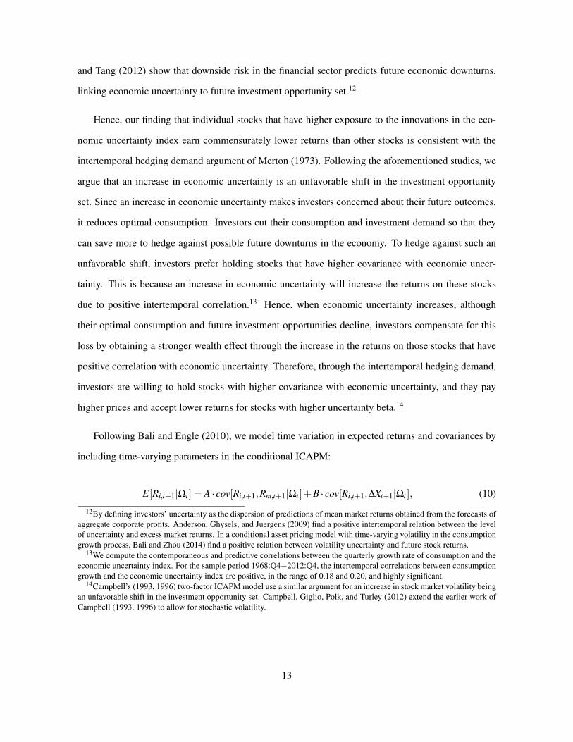
and Tang (2012) show that downside risk in the financial sector predicts future economic downturns,

linking economic uncertainty to future investment opportunity set.12

Hence, our finding that individual stocks that have higher exposure to the innovations in the eco-

nomic uncertainty index earn commensurately lower returns than other stocks is consistent with the

intertemporal hedging demand argument of Merton (1973). Following the aforementioned studies, we

argue that an increase in economic uncertainty is an unfavorable shift in the investment opportunity

set. Since an increase in economic uncertainty makes investors concerned about their future outcomes,

it reduces optimal consumption. Investors cut their consumption and investment demand so that they

can save more to hedge against possible future downturns in the economy. To hedge against such an

unfavorable shift, investors prefer holding stocks that have higher covariance with economic uncer-

tainty. This is because an increase in economic uncertainty will increase the returns on these stocks

due to positive intertemporal correlation.13 Hence, when economic uncertainty increases, although

their optimal consumption and future investment opportunities decline, investors compensate for this

loss by obtaining a stronger wealth effect through the increase in the returns on those stocks that have

positive correlation with economic uncertainty. Therefore, through the intertemporal hedging demand,

investors are willing to hold stocks with higher covariance with economic uncertainty, and they pay

higher prices and accept lower returns for stocks with higher uncertainty beta.14

Following Bali and Engle (2010), we model time variation in expected returns and covariances by

including time-varying parameters in the conditional ICAPM:

E[Ri,t+1|Ωt ] = A · cov[Ri,t+1,Rm,t+1|Ωt ]+B · cov[Ri,t+1,∆Xt+1|Ωt ], (10)

12By defining investors’ uncertainty as the dispersion of predictions of mean market returns obtained from the forecasts ofaggregate corporate profits. Anderson, Ghysels, and Juergens (2009) find a positive intertemporal relation between the levelof uncertainty and excess market returns. In a conditional asset pricing model with time-varying volatility in the consumptiongrowth process, Bali and Zhou (2014) find a positive relation between volatility uncertainty and future stock returns.

13We compute the contemporaneous and predictive correlations between the quarterly growth rate of consumption and theeconomic uncertainty index. For the sample period 1968:Q4−2012:Q4, the intertemporal correlations between consumptiongrowth and the economic uncertainty index are positive, in the range of 0.18 and 0.20, and highly significant.

14Campbell’s (1993, 1996) two-factor ICAPM model use a similar argument for an increase in stock market volatility beingan unfavorable shift in the investment opportunity set. Campbell, Giglio, Polk, and Turley (2012) extend the earlier work ofCampbell (1993, 1996) to allow for stochastic volatility.

13

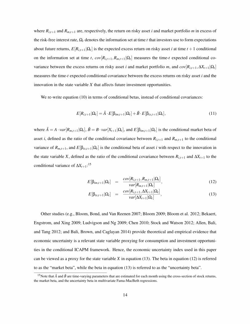
where Ri,t+1 and Rm,t+1 are, respectively, the return on risky asset i and market portfolio m in excess of

the risk-free interest rate, Ωt denotes the information set at time t that investors use to form expectations

about future returns, E[Ri,t+1|Ωt ] is the expected excess return on risky asset i at time t +1 conditional

on the information set at time t, cov[Ri,t+1,Rm,t+1|Ωt ] measures the time-t expected conditional co-

variance between the excess returns on risky asset i and market portfolio m, and cov[Ri,t+1,∆Xt+1|Ωt ]

measures the time-t expected conditional covariance between the excess returns on risky asset i and the

innovation in the state variable X that affects future investment opportunities.

We re-write equation (10) in terms of conditional betas, instead of conditional covariances:

E[Ri,t+1|Ωt ] = A ·E[βim,t+1|Ωt ]+ B ·E[βix,t+1|Ωt ], (11)

where A = A · var[Rm,t+1|Ωt ], B = B · var[Xt+1|Ωt ], and E[βim,t+1|Ωt ] is the conditional market beta of

asset i, defined as the ratio of the conditional covariance between Ri,t+1 and Rm,t+1 to the conditional

variance of Rm,t+1, and E[βix,t+1|Ωt ] is the conditional beta of asset i with respect to the innovation in

the state variable X , defined as the ratio of the conditional covariance between Ri,t+1 and ∆Xt+1 to the

conditional variance of ∆Xt+1:15

E[βim,t+1|Ωt ] =cov[Ri,t+1,Rm,t+1|Ωt ]

var[Rm,t+1|Ωt ], (12)

E[βix,t+1|Ωt ] =cov[Ri,t+1,∆Xt+1|Ωt ]

var[∆Xt+1|Ωt ], (13)

Other studies (e.g., Bloom, Bond, and Van Reenen 2007; Bloom 2009; Bloom et al. 2012; Bekaert,

Engstrom, and Xing 2009; Ludvigson and Ng 2009; Chen 2010; Stock and Watson 2012; Allen, Bali,

and Tang 2012; and Bali, Brown, and Caglayan 2014) provide theoretical and empirical evidence that

economic uncertainty is a relevant state variable proxying for consumption and investment opportuni-

ties in the conditional ICAPM framework. Hence, the economic uncertainty index used in this paper

can be viewed as a proxy for the state variable X in equation (13). The beta in equation (12) is referred

to as the “market beta”, while the beta in equation (13) is referred to as the “uncertainty beta”.

15Note that A and B are time-varying parameters that are estimated for each month using the cross-section of stock returns,the market beta, and the uncertainty beta in multivariate Fama-MacBeth regressions.

14

4. Empirical results

In this section, we conduct parametric and nonparametric tests to assess the predictive power of eco-

nomic uncertainty betas over future stock returns. First, we start with univariate portfolio-level analy-

ses. Second, we discuss average portfolio characteristics to obtain a clear picture of the composition

of uncertainty beta portfolios. Third, we conduct bivariate portfolio-level analyses to examine the

predictive power of uncertainty betas after controlling for well-known stock characteristics and risk

factors. Fourth, we present the univariate and multivariate cross-sectional regression results. Finally,

we provide the results from a battery of robustness checks.

4.1. Univariate portfolio-level analysis

Exposures of individual stocks to macroeconomic uncertainty are obtained from quarterly rolling re-

gressions of excess stock returns on the economic uncertainty index using a 20-quarter fixed window

estimation. The first set of uncertainty betas (βUNC) are obtained using the sample from 1968:Q4 to

1973:Q3. Then, these quarterly uncertainty betas are used to predict the monthly cross-sectional stock

returns in the following three months (October 1973, November 1973, and December 1973). This

quarterly rolling regression approach is used until the sample is exhausted in December 2012. The

cross-sectional return predictability results are reported from October 1973 to December 2012.

Table 1 presents the univariate portfolio results. For each month, we form decile portfolios by

sorting individual stocks based on their uncertainty betas (βUNC), where decile 1 contains stocks with

the lowest βUNC during the past quarter, and decile 10 contains stocks with the highest βUNC during

the previous quarter. The first column in Table 1 reports the average uncertainty betas for the decile

portfolios formed on βUNC using the CRSP breakpoints with equal numbers of stocks in the decile

portfolios. The last four columns in Table 1 present the average excess returns and the 4-factor alphas

on the value-weighted and equal-weighted portfolios.

The first column of Table 1 shows that when moving from decile 1 to decile 10, there is significant

cross-sectional variation in the average values of βUNC; the average uncertainty beta increases from

−22.70 to 26.06. Another notable point in Table 1 is that for the value-weighted portfolio, the next-

month average excess return decreases almost monotonically from 0.98% to 0.32% per month, when

15

moving from the lowest βUNC to the highest βUNC decile. The average return difference between decile

10 (high-βUNC) and decile 1 (low-βUNC) is −0.66% per month with a Newey-West (1987) t-statistic of

−2.75. This result indicates that stocks in the lowest βUNC decile generate about 7.92% higher annual

returns compared to stocks in the highest βUNC decile.

In addition to the average raw returns, Table 1 presents the magnitude and statistical significance of

the difference in intercepts (Fama-French-Carhart, or FFC, four factor alphas) from the regression of

the high-minus-low portfolio returns on a constant, excess market returns (MKT), a size factor (SMB),

a book-to-market factor (HML), and a momentum factor (MOM), following Fama and French (1993)

and Carhart (1997).16 As shown in the third column of Table 1, for the value-weighted portfolio, the

4-factor (FFC) alpha decreases almost monotonically from 0.44% to−0.33% per month, when moving

from the lowest βUNC to the highest βUNC decile. The difference in alphas between the high-βUNC and

low-βUNC portfolios is -0.77% per month with a Newey-West t-statistic of −2.99. This indicates that

after controlling for the well-known size, book-to-market, and momentum factors, the return difference

between the high-βUNC and low-βUNC stocks remains negative and statistically significant.

The last two columns of Table 1 show that similar results are obtained from the equal-weighted

portfolios of βUNC. The average excess returns and the FFC alphas on the uncertainty beta portfolios

decrease almost monotonically. The average return and alpha differences between the high-βUNC and

low-βUNC portfolios are about the same, −0.58% per month, and highly significant with Newey-West

t-statistics larger than 3 in absolute magnitude.

Next, we investigate the source of risk-adjusted return differences between the high-βUNC and low-

βUNC portfolios: Is it due to outperformance by low-βUNC stocks, or underperformance by high-βUNC

stocks, or both? For this, we focus on the economic and statistical significance of the risk-adjusted

returns of decile 1 vs. decile 10. As reported in Table 1, for both value-weighted and equal-weighted

portfolios, the FFC alphas of stocks in decile 1 (low-βUNC stocks) are significantly positive, whereas the

FFC alphas of stocks in decile 10 (high-βUNC stocks) are significantly negative. Hence, we conclude

16SMB (small minus big), HML (high minus low), and MOM (winner minus loser) are described in and obtained fromKenneth French’s data library: http://mba.tuck.dartmouth.edu/pages/faculty/ken.french/.

16

that the significantly negative alpha spreads between high-βUNC and low-βUNC stocks is due to both the

outperformance by low-βUNC stocks and the underperformance by high-βUNC stocks.17

Of course, the economic uncertainty betas documented in Table 1 are for the portfolio formation

month, not for the subsequent month over which we measure average returns. Investors may pay

high prices for stocks that have exhibited high uncertainty beta in the past in the expectation that this

behavior will be repeated in the future, but a natural question is whether these expectations are rational.

Table A2 of the online appendix investigates this issue by presenting the average quarter-to-quarter

portfolio transition matrix. Specifically, Panel A of Table A2 presents the average probability that a

stock in decile i (defined by the rows) in one quarter will be in decile j (defined by the columns) in

the subsequent quarter. If the uncertainty betas were completely random, then all the probabilities

should be approximately 10%, since a high or low uncertainty beta in one quarter should say nothing

about the uncertainty beta in the following quarter. Instead, all the diagonal elements of the transition

matrix exceed 10%, illustrating that the uncertainty beta is highly persistent. Of greater importance,

this persistence is especially strong for the extreme portfolios. Panel A shows that for the one-quarter

ahead persistence of βUNC, stocks in decile 1 (decile 10) have a 73.95% (73.53%) chance of appearing

in the same decile next quarter. Similarly, Panel D of Table A2 shows that for the four-quarter ahead

persistence of βUNC, stocks in decile 1 (decile 10) have a 54.03% (54.68%) chance of appearing in the

same decile next four quarters.18

These results indicate that the estimated historical uncertainty betas successfully predict future

uncertainty betas and hence they are good proxies for the true conditional betas, which is important

for interpretations of the results in terms of an equilibrium model such as the ICAPM. These results

also show that the uncertainty betas are not simply characteristics of firms that result in differences in

expected returns, but they are proxies for a source of macroeconomic uncertainty.

17As shown in Table A3 of the online appendix, very similar results are obtained when decile portfolios are formed basedon the NYSE breakpoints, which are used to alleviate the concerns that the CRSP decile breakpoints are distorted by the largenumber of small Nasdaq and Amex stocks (Fama and French, 1992).

18Note that stocks in decile 1 have about 74% probability of being in deciles 1-2, all of which exhibit low uncertainty betain the portfolio formation month and high returns in the subsequent month. Similarly, stocks in decile 10 have about 72%probability of being in deciles 9−10, all of which exhibit high uncertainty beta in the portfolio formation month and lowreturns in the subsequent month.

17

4.2. Average portfolio characteristics

To obtain a clearer picture of the composition of the uncertainty beta portfolios, Table 2 presents sum-

mary statistics for the stocks in the deciles. Specifically, Table 2 reports the cross-sectional averages

of various characteristics for the stocks in each decile averaged across the months. We report average

values for the uncertainty beta (βUNC), the market share (Mkt. shr.), the market beta (BETA), the log

market capitalization (SIZE), the log book-to-market ratio (BM), the return over the 11 months prior to

portfolio formation (MOM), the return in the portfolio formation month (REV), a measure of illiquidity

(ILLIQ), co-skewness (COSKEW), idiosyncratic volatility (IVOL), analyst dispersion (DISP), firm age

(AGE), leverage (LEV), and the price in dollars (PRC). The definitions of these variables are given in

Section 2.3.

The portfolios exhibit interesting patterns. Average market betas are higher for the low-βUNC and

high-βUNC portfolios, compared to deciles 2 to 9. Not surprisingly, stocks in the high-βUNC portfolio

have somewhat higher market betas than those in the low-βUNC portfolio. Stocks in the extreme deciles

(deciles 1 and 10) are relatively smaller compared to those in deciles 2 to 9. As expected, the last

column of Table 2 shows that stocks in the low-βUNC and high-βUNC portfolios have somewhat lower

share prices compared to those in deciles 2 to 9, but there is no monotonically increasing or decreasing

pattern in the average prices of the stocks in the uncertainty beta portfolios. Average book-to-market

and leverage ratios are lower for the low-βUNC and high-βUNC portfolios, compared to deciles 2 to 9.

Since there is no significant difference between the size, value, and leverage characteristics of stocks

in the low-βUNC and high-βUNC portfolios, the predictive power of the uncertainty beta cannot be

explained by size, book-to-market, and distress risk.

A notable point in Table 1 is that stocks in the extreme deciles (deciles 1 and 10) have higher

past one year returns, that is, stocks in the low-βUNC and high-βUNC portfolios are momentum winners

compared to those in deciles 2 to 9. Since there is no monotonically increasing or decreasing pattern in

the past one year return of uncertainty portfolios, momentum cannot be an explanation for the predictive

power of the uncertainty beta either.

18

Interestingly, stocks in the extreme deciles (deciles 1 and 10) have higher past one month returns

as well, that is, stocks in the low-βUNC and high-βUNC portfolios are short-term winners compared to

those in deciles 2 to 9. But again there is no monotonically increasing or decreasing pattern in the past

one month return of the uncertainty beta portfolios. Hence, short-term reversal cannot explain the high

(low) returns on low (high) uncertainty beta stocks.

There are no significant differences in the liquidity, idiosyncratic volatility, analyst dispersion, and

firm age of average stocks in the low-βUNC and high-βUNC portfolios, but consistent with earlier studies,

small and lower-priced stocks in the low-βUNC and high-βUNC portfolios are somewhat more volatile,

illiquid, younger, and have a higher analyst dispersion compared to those in deciles 2 to 9. However, the

differences in the liquidity, volatility, dispersion, and age of stocks in deciles 1 and 10 are so trivial that

similar to our findings for size, price, value, leverage, momentum, and reversal effects, the liquidity,

volatility, dispersion, and age cannot explain the return predictability of the uncertainty beta.

The only variable that seems to have a strong correlation with the uncertainty beta (at the portfolio

level) is co-skewness. When moving from the low-βUNC to the high-βUNC portfolios, average co-

skewness increases monotonically from −0.09 to −0.02. Harvey and Siddique (2000) find that stocks

with high co-skewness generate low returns. Hence, co-skewness may potentially explain the high

(low) returns on low (high) uncertainty beta stocks.

We address this potential concern in the following two sections. Although there are no striking pat-

terns in average portfolio characteristics (with the exception of co-skewness), in the following sections,

we provide different ways of dealing with the potential interaction of the uncertainty beta with the mar-

ket beta, size, book-to-market, momentum, short-term reversal, liquidity, co-skewness, idiosyncratic

volatility, analyst dispersion, firm age, and leverage. Specifically, we test whether the negative relation

between the economic uncertainty beta and the cross-section of expected returns still holds once we

control for the usual suspects using bivariate portfolio sorts and Fama-MacBeth (1973) regressions.

4.3. Bivariate portfolio-level analysis

This section examines the relation between the uncertainty beta and future stock returns after control-

ling for well-known cross-sectional return predictors. We perform bivariate portfolio sorts on the eco-

19

nomic uncertainty beta (βUNC) in combination with the market beta (BETA), the log market capitaliza-

tion (SIZE), the log book-to-market ratio (BM), momentum (MOM), short-term reversal (REV), illiq-

uidity (ILLIQ), co-skewness (COSKEW), idiosyncratic volatility (IVOL), analyst dispersion (DISP),

firm age (AGE), and leverage (LEV). Table 3 reports the value-weighted portfolio results of these con-

ditional bivariate sorts.

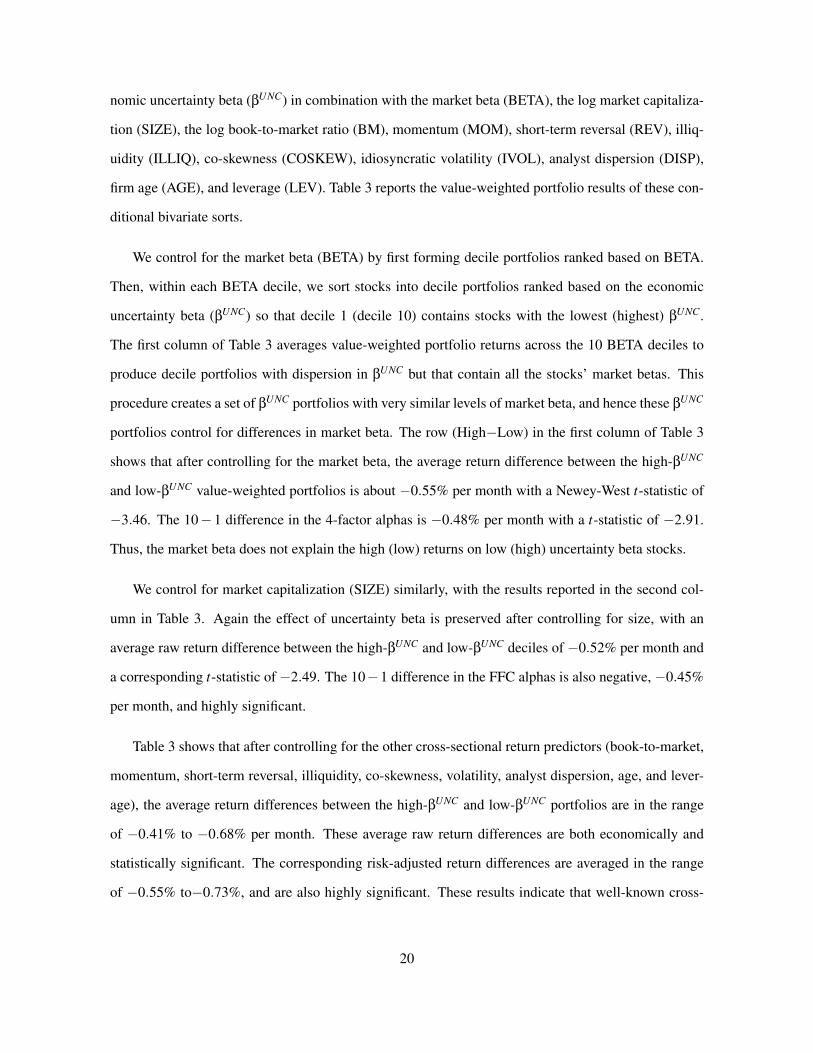
We control for the market beta (BETA) by first forming decile portfolios ranked based on BETA.

Then, within each BETA decile, we sort stocks into decile portfolios ranked based on the economic

uncertainty beta (βUNC) so that decile 1 (decile 10) contains stocks with the lowest (highest) βUNC.

The first column of Table 3 averages value-weighted portfolio returns across the 10 BETA deciles to

produce decile portfolios with dispersion in βUNC but that contain all the stocks’ market betas. This

procedure creates a set of βUNC portfolios with very similar levels of market beta, and hence these βUNC

portfolios control for differences in market beta. The row (High−Low) in the first column of Table 3

shows that after controlling for the market beta, the average return difference between the high-βUNC

and low-βUNC value-weighted portfolios is about −0.55% per month with a Newey-West t-statistic of

−3.46. The 10− 1 difference in the 4-factor alphas is −0.48% per month with a t-statistic of −2.91.

Thus, the market beta does not explain the high (low) returns on low (high) uncertainty beta stocks.

We control for market capitalization (SIZE) similarly, with the results reported in the second col-

umn in Table 3. Again the effect of uncertainty beta is preserved after controlling for size, with an

average raw return difference between the high-βUNC and low-βUNC deciles of −0.52% per month and

a corresponding t-statistic of −2.49. The 10−1 difference in the FFC alphas is also negative, −0.45%

per month, and highly significant.

Table 3 shows that after controlling for the other cross-sectional return predictors (book-to-market,

momentum, short-term reversal, illiquidity, co-skewness, volatility, analyst dispersion, age, and lever-

age), the average return differences between the high-βUNC and low-βUNC portfolios are in the range

of −0.41% to −0.68% per month. These average raw return differences are both economically and

statistically significant. The corresponding risk-adjusted return differences are averaged in the range

of −0.55% to−0.73%, and are also highly significant. These results indicate that well-known cross-

20

sectional effects (including co-skewness) cannot explain the low returns to stocks with high uncertainty

beta.

4.4. Stock level cross-sectional regressions

So far we have tested the significance of the economic uncertainty beta as a determinant of the cross-

section of future returns at the portfolio level. This portfolio-level analysis has the advantage of being

nonparametric in the sense that we do not impose a functional form on the relation between uncertainty

betas and future returns. The portfolio-level analysis also has two potentially significant disadvantages.

First, it throws away a large amount of information in the cross-section via aggregation. Second, it is

a difficult setting in which to control for multiple effects or factors simultaneously. Consequently, we

now examine the cross-sectional relation between the uncertainty beta and expected returns at the stock

level using the Fama and MacBeth (1973) regressions.

We present the time-series averages of the slope coefficients from the regressions of one-month

ahead stock returns on the economic uncertainty beta (βUNC) with and without control variables. The

average slopes provide standard Fama-MacBeth tests for determining which explanatory variables on

average have non-zero premiums. Monthly cross-sectional regressions are run for the following econo-

metric specification and nested versions thereof:

Ri,t+1 = λ0,t +λ1,t ·βUNCi,t +λ2,t ·Xi,t + εi,t+1, (14)

where Ri,t+1 is the realized return on stock i in month t + 1, βUNCi,t is the quarterly economic uncer-

tainty beta of stock i in months t, t − 1, and t − 2, and Xi,t is a collection of stock-specific control

variables observable at time t for stock i (market beta, size, book-to-market, momentum, short-term

reversal, illiquidity, co-skewness, idiosyncratic volatility, analyst dispersion, age, and leverage). The

cross-sectional regressions are run at a monthly frequency from October 1973 to December 2012.

When calculating the standard errors of the average slope coefficients, we take into account autocorre-

lation and heteroscedasticity in the time-series slope coefficients from cross-sectional regressions. The

Newey-West (1987) adjusted standard errors are computed with six lags.

21

Panel A of Table 4 reports the time series averages of the slope coefficients and the Newey-West

t-statistics in parentheses. The univariate regression results reported in the first column indicate a

negative and statistically significant relation between the economic uncertainty beta and the cross-

section of future stock returns. The average slope from the monthly regressions of realized returns on

βUNCi,t alone is −0.016 with a t-statistic of −3.37.

To delineate the economic significance of this average slope coefficient, we use the average values

of the uncertainty betas in the decile portfolios. Table 1 shows that the difference in βUNCi,t values

between average stocks in the first and 10th deciles is 48.76[= 26.06− (−22.70)]. If a stock were to

move from the first to the 10th decile of βUNCi,t , what would be the change in that stock’s expected return?

The average slope coefficient of −0.016 on βUNCi,t in Panel A of Table 4 represents an economically

significant decrease of−0.016×48.76 =−0.78% per month in the average stock’s expected return for

moving from the first to the 10th decile of βUNCi,t .

The second column in Panel A of Table 4 controls for the market beta (BETA), market capitalization

(SIZE), and the book-to-market (BM), a cross-sectional regression specification corresponding to the 3-

factor model of Fama and French (1993). The third column controls for the market beta (BETA), market

capitalization (SIZE), the book-to-market (BM), and momentum (MOM), a cross-sectional regression

specification corresponding to the 4-factor model of Fama and French (1993) and Carhart (1997). In

both specifications, the average slopes from the monthly regressions of realized returns on βUNCi,t are

negative and highly significant; −0.014 and−0.012 with Newey-West t-statistics of−3.80 and−3.64,

respectively.

Column (4) controls for all variables (except for age and leverage) simultaneously, including the

market beta, size, the book-to-market, momentum, short-term reversal, illiquidity, co-skewness, id-

iosyncratic volatility, analyst dispersion, age, and leverage. In this more general specification, the

average slope of βUNCi,t remains negative, −0.011, and highly significant with a Newey-West t-statistic

of−4.50. The average slope coefficient of−0.011 for βUNCi,t implies that a portfolio short-selling stocks

with the highest uncertainty beta (stocks in decile 10) and buying stocks with the lowest uncertainty

beta (stocks in decile 1) generates a return in the following month of about 0.54%, controlling for ev-

22

erything else. The last column includes firm age and leverage to a large set of controls, and the main

findings remain intact.

In general, the coefficients of the individual control variables are also as expected; the size effect

is negative and significant, the value effect is positive and significant, stocks exhibit intermediate-

term momentum and short-term reversals, and the average slopes of idiosyncratic volatility and analyst

dispersion are negative and significant. The average slope of the market beta (BETA) is positive but

statistically insignificant, which contradicts the implications of the CAPM but is consistent with prior

empirical evidence. The average slope of co-skewness is negative but statistically insignificant. The

average slope of illiquidity is negative and significant, contradicting the positive illiquidity premium

identified by earlier studies. The average slope coefficients on firm age and leverage are statistically

insignificant because they are correlated with some of the control variables such as firm size and book-

to-market.19

In Panel B of Table 4, we control for the industry effect. For each month, we assign each stock to

one of the 10 industries based on the four-digit SIC code and replicate our firm-level cross-sectional

regressions with and without the large set of firm characteristics and risk factors.

The univariate regression results reported in the first column of Table 4, Panel B indicate a negative

and statistically significant relation between the uncertainty beta and future stock returns after control-

ling for the industry effect; the average slope coefficient is −0.014 with a Newey-West t-statistic of

−3.64. As expected, the average slope on βUNC is somewhat smaller in absolute magnitude (−0.014

in Panel B vs. −0.016 in Panel A) after controlling for the industry effect. However, the average slope

of −0.014 still represents an economically significant decrease of −0.68% per month in the average

stock’s expected return for moving from the first to the 10th decile of βUNC.

The last four columns in Panel B of Table 4 examines the significance of uncertainty beta after

controlling for the industry effect and a sequential set of other cross-sectional predictors. Columns

19In the online appendix, we replicate multivariate Fama-MacBeth regressions with standardized residuals for each disper-sion measure separately. Table A4 shows that the average slope coefficients on each component of UNCAV G are negative andstatistically significant, indicating that our main findings hold for individual measures of economic uncertainty. These resultsalso imply that all seven measures of dispersion in economic forecasts (i.e., output, inflation, and unemployment) contributesignificantly to the predictability of stock returns.

23

(2) and (3) show that when controlling for the industry as well as the size, book-to-market and mo-

mentum effects, the average slopes from the monthly regressions of returns on βUNC are negative and

highly significant; −0.013 and −0.011 with t-statistics of −3.77 and −3.76, respectively. The last

two columns present results from the more general specifications including all other control variables

along with the industry effect. As shown in Columns (4) and (5), the average slope of βUNC remains

negative at −0.009 and highly significant. The average slope coefficient of −0.009 for βUNC implies

that a portfolio short-selling stocks with the highest uncertainty beta and buying stocks with the lowest

uncertainty beta generates a return in the following month of about 0.44%, controlling for the industry

effect and everything else.20

Finally, we test whether the economic uncertainty beta remains significant in multivariate Fama-

MacBeth regressions after controlling for the betas with respect to the Fama-French-Carhart factors.

For each month from October 1968 to December 2012, we estimate the Fama-French-Carhart model

using a 60-month rolling window with a minimum of 24 observations and updated monthly:

Ri,t = αi,t +βMKTi,t ·Rm,t +β

SMBi,t ·SMBt +β

HMLi,t ·HMLt +β

MOMi,t ·MOMt + εi,t , (15)

and then control for βMKTi , βSMB

i , βHMLi , and βMOM

i simultaneously.

Panel C of Table 4 shows that the average slopes on βUNC remains negative, in the range of−0.013

and −0.009, and highly significant after controlling for the betas with respect to the Fama-French-

Carhart factors along with the other firm characteristics (short-term reversal, illiquidity, co-skewness,

idiosyncratic volatility, dispersion, age, and leverage). In general, the coefficients of the individual

control variables in Panel C are similar to those reported in Panel A and B of Table 4. The only

exceptions are firm age and leverage. The last column of Panel C shows that the average slope on

AGE is negative and significant, indicating higher average return on younger firms. The average slope

20At an earlier stage of the study, we replicate our main finding using the value-weighted 38 and 48 industry portfolios ofFama and French (1997). We first estimate exposures of the industry portfolios to the economic uncertainty index (βUNC)and then form univariate value-weighted portfolios based on βUNC

ind . Table A5 of the online appendix shows that the averagereturn and alpha differences between the high-βUNC

ind and low-βUNCind portfolios are negative and significant, indicating that the

negative uncertainty premium is prevalent in the cross-section of industry portfolios as well.

24

on LEV is positive and marginally significant, indicating higher average return on firms with higher

leverage.

4.5. Robustness check

In this section, we summarize empirical findings from a battery of robustness checks. The results are

reported in Tables A6−A11 of the online appendix.

4.5.1. Subsample analysis

First, we investigate whether our results are sensitive to different stock samples. As discussed in Sec-

tion 2.3, our original sample includes all common stocks traded on the NYSE, Amex, and Nasdaq

exchanges. We further investigate whether our results are driven by small, low-priced, and illiquid

stocks, or stocks trading at the Amex and Nasdaq exchanges. The sensitivity of our main findings is

tested for seven different stock samples: (i) NYSE stocks only; (ii) Large stocks, defined as those with

market capitalization greater than the 50th NYSE size percentile at the beginning of each month; (iii)

S&P 500 stocks; (iv) The largest 500 stocks in the CRSP universe, based on the market capitalization;

(v) The largest 1,000 stocks in the CRSP universe, based on the market capitalization; (vi) The most

liquid 500 stocks in the CRSP universe, based on Amihud’s (2002) illiquidity measure; and (vii) The

most liquid 1,000 stocks in the CRSP universe, based on Amihud’s (2002) illiquidity measure. We

replicate our main findings for these seven different stock samples based on the value-weighted port-

folios. As shown in Table A6 of the online appendix, our main findings hold for all stock samples

considered in the paper; the FFC alpha spread between the high-βUNC and low-βUNC portfolios is in the

range of −0.47% and −0.62% per month and statistically significant for the NYSE stocks, and S&P

500 stocks, and large and liquid stocks.

4.5.2. Subperiod analysis

We now test whether our findings are robust across different time periods. Since the original data on the

cross-sectional dispersion in economic forecasts provided by the Federal Reserve Bank of Philadelphia

cover the period 1968:Q4 to 2012:Q4, the cross-sectional return predictability results are based on the

25

sample period from October 1973 to December 2012. The first two columns of Table A7 in the online

appendix shows that the cross-sectional return predictability results are robust across the two subsample

periods. Although the FFC alpha spreads between the high-βUNC and low-βUNC portfolios are negative

and significant for both subperiods, the FFC alpha spread is larger for the second subperiod with more

severe economic and market downturns, compared to the first subperiod; −0.97% per month for June

1993−December 2012 vs. −0.58% per month for October 1973−May 1993.

4.5.3. Recessions vs. expansions

In this section, we examine whether the macroeconomic uncertainty premium is higher during reces-

sions in which economic activity (including investment and consumption) is low and the marginal util-

ity of wealth is high. We determine states of the economy based on the Chicago FED National Activity

Index (CFNAI)21 and the National Bureau of Economic Research (NBER) recession dummy taking the

value of one if the U.S. economy is in recession in a month as determined by the NBER. Table A8 of the

online appendix shows that the uncertainty premium is much higher when the CFNAI index is below

−0.7 and during the NBER recession months. These results are consistent with the intertemporal cap-

ital asset pricing models of Merton (1973) and Campbell (1993, 1996). During economic downturns,

ICAPM investors are more concerned about potential declines in their consumption and investment

opportunities. Because of elevated fear and uncertainty during downturns of the economy, investors

cut their investment and consumption demand. To compensate for this loss, they prefer to hold stocks

that have high covariance with economic uncertainty (stocks with high uncertainty beta) because when

uncertainty increases, the returns of high uncertainty beta stocks increase and generate an additional

wealth effect that compensates for the loss in consumption. Thus, investors increase their intertemporal

hedging demand even further when economic uncertainty is high during recessions and they are willing

to accept lower expected returns for hedging purposes. The empirical results in Table A8 are consistent

21The CFNAI is a monthly index designed to assess overall economic activity and related inflationary pressure. It is theweighted average of 85 existing monthly indicators of national economic activity. It is constructed to have an average valueof zero and a standard deviation of one. Since economic activity tends toward the trend growth rate over time, a positiveindex reading corresponds to growth above the trend and a negative index reading corresponds to growth below the trend. ACFNAI index value below −0.7 following a period of economic expansion indicates an increasing likelihood that a recessionhas begun.

26

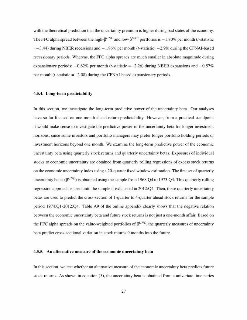
with the theoretical prediction that the uncertainty premium is higher during bad states of the economy.

The FFC alpha spread between the high-βUNC and low-βUNC portfolios is−1.80% per month (t-statistic

=−3.44) during NBER recessions and−1.86% per month (t-statistic=−2.98) during the CFNAI-based

recessionary periods. Whereas, the FFC alpha spreads are much smaller in absolute magnitude during

expansionary periods; −0.62% per month (t-statistic =−2.26) during NBER expansions and −0.57%

per month (t-statistic =−2.08) during the CFNAI-based expansionary periods.

4.5.4. Long-term predictability

In this section, we investigate the long-term predictive power of the uncertainty beta. Our analyses

have so far focused on one-month ahead return predictability. However, from a practical standpoint

it would make sense to investigate the predictive power of the uncertainty beta for longer investment

horizons, since some investors and portfolio managers may prefer longer portfolio holding periods or

investment horizons beyond one month. We examine the long-term predictive power of the economic

uncertainty beta using quarterly stock returns and quarterly uncertainty betas. Exposures of individual

stocks to economic uncertainty are obtained from quarterly rolling regressions of excess stock returns

on the economic uncertainty index using a 20-quarter fixed window estimation. The first set of quarterly

uncertainty betas (βUNC) is obtained using the sample from 1968:Q4 to 1973:Q3. This quarterly rolling

regression approach is used until the sample is exhausted in 2012:Q4. Then, these quarterly uncertainty

betas are used to predict the cross-section of 1-quarter to 4-quarter ahead stock returns for the sample

period 1974:Q1-2012:Q4. Table A9 of the online appendix clearly shows that the negative relation

between the economic uncertainty beta and future stock returns is not just a one-month affair. Based on

the FFC alpha spreads on the value-weighted portfolios of βUNC, the quarterly measures of uncertainty

beta predict cross-sectional variation in stock returns 9 months into the future.

4.5.5. An alternative measure of the economic uncertainty beta

In this section, we test whether an alternative measure of the economic uncertainty beta predicts future

stock returns. As shown in equation (5), the uncertainty beta is obtained from a univariate time-series

27

regression of excess stock returns on the economic uncertainty index. We now estimate the uncertainty

beta controlling for the market factor. Specifically, for each stock and for each quarter, we estimate

the uncertainty beta from the quarterly rolling regressions of excess stock returns on the economic

uncertainty index and the excess market return over a 20-quarter fixed window period:

Ri,t = αi,t +βUNCi,t ·UNCAV G

t +βMKTi,t ·Rm,t + εi,t , (16)

where Ri,t is the excess return on stock i, Rm,t is the excess market return, and UNCAV Gt is the economic

uncertainty index defined as the average of the standardized residuals from the AR(1) model for the

seven dispersion measures.

Table A10 of the online appendix presents the time-series averages of the slope coefficients from the

cross-sectional regressions of one-month ahead stock returns on the economic uncertainty beta (βUNCi,t )

and the market beta (βMKTi,t ) obtained from equation (16) plus the control variables. Monthly cross-

sectional regressions are run for the following econometric specification and nested versions thereof:

Ri,t+1 = λ0,t +λ1,t ·βUNCi,t +λ2,t ·βMKT

i,t +λ3,t ·Xi,t + εi,t , (17)

Similar to our findings in Panel A of Table 4, the average slope coefficients on βUNCi are negative, in

the range of −0.012 and −0.016, and significant with Newey-West t-statistics ranging from −3.14 to

−4.77. In general, the coefficients of the individual control variables are very similar to those presented

in Table 4, Panel A. The only exception is the market beta. The last two columns of Table A10 show

that the average slope on βMKTi is positive and marginally significant in some of the specifications

controlling for βUNCi and firm characteristics.

4.5.6. An alternative measure of the economic uncertainty index

As discussed in Section 2.2, we introduce an alternative measure of the economic uncertainty index

based on the first principal component of the standardized residuals from AR(1) regressions for the

seven dispersion measures. In this section, we test if this alternative measure of the uncertainty index

28

affects our main findings. Specifically, for each stock and for each quarter, we estimate the uncer-

tainty beta from the quarterly rolling regressions of excess stock returns on the PCA-based economic

uncertainty index (UNCPCAt ) over a 20-quarter fixed window period:

Ri,t = αi,t +βUNCi,t ·UNCPCA

t + εi,t . (18)

Table A11 of the online appendix presents the time-series averages of the slope coefficients from

the Fama-MacBeth cross-sectional regressions of one-month ahead stock returns on the alternative

measure of the uncertainty beta (βUNCi ) obtained from equation (18) plus the control variables. Similar

to our findings in Panel A of Table 4, the average slope coefficients on βUNCi are negative, in the range of

-0.041 and -0.032, and significant with Newey-West t-statistics ranging from 3.21 to 4.45. In general,

the coefficients of the individual control variables are very similar to those presented in Table 4, Panel

A. Overall, these results indicate that the cross-sectional predictive power of economic uncertainty

remains intact when we replace UNCAV Gt with UNCPCA

t in the estimation of the uncertainty beta.

5. Controlling for Exposure to Stock Market Volatility

Campbell (1993, 1996) provides a two-factor ICAPM in which an unexpected increase in market

volatility represents deterioration in the investment opportunity set or a decrease in optimal consump-

tion. In this setting, a positive covariance of returns with volatility shocks (or innovations in market

volatility) predicts a lower return on the stock. In the context of Campbell’s ICAPM, an increase in

market volatility predicts a decrease in optimal consumption and hence an unfavorable shift in the

investment opportunity set. Risk-averse investors will demand more of a stock, the more positively

correlated the stock’s return is with changes in market volatility because they will be compensated by

a higher level of wealth through the positive correlation of the returns. That stock can be viewed as a

hedging instrument. In other words, an increase in the covariance of returns with volatility risk leads

to an increase in the hedging demand, which in equilibrium reduces expected return on the stock.22

22Campbell et al. (2012), extending the earlier work of Campbell (1993, 1996), estimate market variance innovationsbased on a vector autoregression approach, and find a negative market variance risk premium in the cross-section of equityportfolios.

29

Ang et al. (2006) test whether the exposure of individual stocks to changes in market volatility

predict cross-sectional variation in future stock returns. They first estimate the exposure of individual

stocks to changes in the S&P 100 index option implied volatility (VXO). Then, they sort stocks into

quintile portfolios based on these implied volatility betas. They find a negative cross-sectional relation

between the volatility betas and future stock returns, that is, stocks with higher (lower) exposure to

changes in the VXO generate lower (higher) returns in the next month. Bali and Engle (2010) investi-

gate the significance of a negative market volatility risk premium in the conditional ICAPM framework

and find that equity portfolios with higher conditional covariance with changes in expected future mar-

ket volatility yield lower expected returns. Coval and Shumway (2001) and Bakshi and Kapadia (2003)

find the volatility risk premium to be negative in equity option markets. Adrian and Rosenberg (2008)

decompose equity market volatility into short- and long-term components and show that the prices of

both components are significantly negative. Bansal, Kiku, Shaliastovich, and Yaron (2014) show that

equities have negative volatility betas and hence equities carry positive volatility risk premia.

In this section, motivated by the aforementioned studies, we test whether the predictive power

of economic uncertainty beta remains intact after controlling for the exposure of individual stocks to

changes in aggregate stock market volatility. Following Ang et al. (2006), we use the VXO as a proxy

for market volatility.

In addition to option implied volatility, we use expected realized market variance to generate an

alternative measure of volatility innovation. Specifically, market variance innovation (∆VARRealizedt )

is defined as the residual from the time-series regression of the realized market variance in quarter

t against a vector of lagged quarterly state variables over the period 1968:Q4−2012:Q4. Following

Campbell, Giglio, Polk, and Turley (2012), the state variables include (i) the log real return on the

market (Rm), defined as the difference between the log return on the CRSP value-weighted stock index

and the log return on the Consumer Price Index (CPI); (ii) the market variance itself (VAR), defined

as the sum of the squared daily returns on the CRSP value-weighted stock index in a quarter; (iii) the

log price-earnings ratio (P/E) of Shiller (2000), constructed as the price of the S&P 500 index divided

by a one-quarter lagged 10-year trailing moving average of aggregate earnings of companies in the

S&P500 index; (iv) the term yield spread (TERM), computed as the difference between the log yield

30

on the 10-year US Constant Maturity Bond and the log yield on the 3-month US Treasury Bill; (v)

the small-stock value spread (VS), constructed following Campbell and Vuolteenaho (2004); and (vi)

the default spread (DEF), calculated as the difference between the log yields on Moody’s BAA and

AAA bonds. Daily and monthly stock market returns are obtained from the CRSP database; the CPI,

Treasury yields, and yields on Moody’s BAA and AAA are downloaded from the Federal Reserve Bank

of St. Louis; data used to calculate P/E are obtained from Robert Shiller’s website; and data used to

measure VS are obtained from Kenneth French’s website.

First, we investigate the potential interaction between the economic uncertainty beta and the market

volatility beta by controlling for the realized and implied market volatility innovations in the estimation

of the uncertainty beta. Specifically, for each stock and for each quarter, we estimate the uncertainty

beta from the quarterly rolling regressions of excess stock returns on the economic uncertainty index

and the change in market volatility over a 20-quarter fixed window period:

Model 1 : Ri,t = αi,t +βUNCi,t ·UNCAV G

t +βRVOLi,t ·∆VARRealized

t + εi,t , (19)

Model 2 : Ri,t = αi,t +βUNCi,t ·UNCAV G

t +βV XOi,t ·∆VARV XO

t + εi,t , (20)

where Ri,t is the excess return on stock i, UNCAV Gt is the economic uncertainty index defined as the aver-

age of the standardized residuals from the AR(1) model for the seven dispersion measures, ∆VARRealizedt

is the change in the expected realized market variance, ∆VARV XOt is the change in the S&P 100 index

option implied variance, and βUNCi , βRVOL

i , and βV XOi are the measures of the economic uncertainty

beta, the expected realized market volatility beta, and the implied market volatility beta, respectively.23

We use two more specifications to control for the market volatility factor and the excess market

return simultaneously in the estimation of the uncertainty beta:

Model 3 : Ri,t = αi,t +βUNCi,t ·UNCAV G

t +βRVOLi,t ·∆VARRealized

t +βMKTi,t ·Rm,t + εi,t , (21)

Model 4 : Ri,t = αi,t +βUNCi,t ·UNCAV G

t +βV XOi,t ·∆VARV XO

t +βMKTi,t ·Rm,t + εi,t , (22)

23We should note that the daily data on the VXO are available from January 2, 1986. Thus, our cross-sectional returnpredictability results from the VXO data are based on the sample period from January 1986 to December 2012.

31

Once we estimate the economic uncertainty beta from Model 1, 2, 3, and 4, we form the value-

weighted decile portfolios by sorting individual stocks based on βUNCi . Panel A of Table 5 shows that

the FFC alpha differences between the high-βUNCi and low-βUNC

i portfolios are negative, in the range

−0.53% and −0.89% per month, and highly significant with Newey-West t-statistics ranging from

−2.19 to−2.91. These results indicate that the predictive power of the uncertainty beta remains highly

significant after accounting for the interaction between the uncertainty beta and the market volatility

beta.

Next, we test whether the predictive power of βUNCi remains intact when controlling for βRVOL

i and

βV XOi in conditional bivariate sorts. Panel B of Table 5 shows that after controlling for the expected

realized market volatility beta (βRVOLi ), the significantly negative link between the uncertainty beta and

future stock returns remains intact. The FFC alpha difference between the high-βUNCi and low-βUNC

i

portfolios is −0.71% per month with a t-statistic of −3.67 when βUNCi and βRVOL

i are estimated with

Model 1, and −0.70% per month with a t-statistic of −3.46 when βUNCi and βRVOL

i are estimated with

Model 3. The last two columns of Table 5, Panel B shows that similar findings are obtained when

we control for the implied volatility beta (βV XOi ). The FFC alpha difference between the high-βUNC

i

and low-βUNCi portfolios is −0.85% per month with a t-statistic of −3.11 when βUNC

i and βV XOi are

estimated with Model 2, and −0.73% per month with a t-statistic of −2.83 when βUNCi and βV XO

i are

estimated with Model 4. These results clearly show that exposure of individual stocks to changes in

market volatility does not diminish the predictive power of the uncertainty beta.

Finally, we examine the predictive power of the uncertainty beta after controlling for the market

volatility beta and firm characteristics in multivariate Fama-MacBeth regressions. In Panel C of Table

5, we re-run the earlier cross-sectional regressions (reported in Table 4, Panel A) with βUNCi , βMKT

i ,

βRVOLi and βV XO

i estimated from Models 1, 2, 3, and 4. The results indicate that after accounting

for the expected realized volatility beta, the implied volatility beta, market beta, and all other control

variables, the average slope of the economic uncertainty beta remains negative and highly significant. In

general, the coefficients of the individual control variables are very similar to those presented in Table

4. A notable point in Table 5, Panel C is that the average slope on βRVOLi and βV XO

i are statistically

32

insignificant, indicating that the negative volatility risk premium is subsumed by the highly significant

negative premium of economic uncertainty.

Portfolio level analyses and cross-sectional regressions provide clear evidence that the predictive

power of the uncertainty beta is not driven by the exposure of individual stocks to changes in market

volatility. We identify a significant negative premium of economic uncertainty in the cross-section of

individual stocks, and that is distinct from the volatility risk premium identified by earlier studies.

6. Alternative Measures of the Economic Uncertainty Index

In this section, we test whether our main findings are robust to alternative measures of the economic

uncertainty index proposed by other studies.

Jurado, Ludvigson, and Ng (2013) use a large number of financial and macroeconomic variables

to provide a new measure of macroeconomic uncertainty, defined as the common variation in the un-

forecastable component of a large number of economic indicators.24 Their empirical analysis forms

forecasts and common uncertainty from this large dataset covering the period January 1959−December

2011. The correlation between the quarterly measure of the economic uncertainty index proposed in

this paper and the quarterly macroeconomic uncertainty measure of Jurado et al. (2013) is 0.37 for the

common sample period from 1968:Q4 to 2011:Q4.

Bali, Brown, and Caglayan (2014) propose alternative measures of macroeconomic risk by estimat-

ing the time-varying conditional volatility of eight macroeconomic variables based on the multivariate

asymmetric GARCH model with a vector autoregressive process.25 Since macroeconomic risk factors

introduced by Bali et al. (2014) are measures of conditional volatility, they are highly persistent and

correlated with each other. To sufficiently capture the common variation among correlated factors of

economic uncertainty, they develop a broad index of macroeconomic risk using principal component

24Jurado, Ludvigson, and Ng (2013) combine the macro and financial monthly datasets used by Ludvigson and Ng (2007,2010). Specifically, the first dataset used by Jurado et al. (2013) is an updated version of the 132 macroeconomic seriesused by Ludvigson and Ng (2010). The second dataset is an updated monthly version of the 147 financial time seriesused by Ludvigson and Ng (2007). Jurado et al. (2013) combine the macro and financial datasets together into one largemacroeconomic dataset to estimate forecasting factors in these 279 (= 132+147) series.

25The macroeconomic variables used by Bali, Brown, and Caglayan (2014) are the default spread, the term spread, thede-trended short-term interest rate, the aggregate dividend yield, the aggregate stock market index, the growth rate of realGDP per capita, the inflation rate, and the unemployment rate.

33

analysis. The correlation between the quarterly measure of the economic uncertainty index proposed

in this paper and the quarterly macroeconomic risk index of Bali et al. (2014) is 0.42 for the common

sample period, 1994:Q1−2012:Q1.

Figure 2 plots the quarterly measures of the economic uncertainty index proposed in this paper,

the macroeconomic uncertainty measure of Jurado, Ludvigson, and Ng (2013), denoted JLN, and the

macroeconomic risk index of Bali, Brown, and Caglayan (2014), denoted BBC. Figure 2 clearly shows

that all three measures of the economic uncertainty index are highly correlated and they closely follow

large fluctuations in business conditions including major economic and financial crises. However, the

economic uncertainty index proposed in this paper UNCAV G has stronger time-series variation.

Since the economic uncertainty indices of Jurado, Ludvigson, and Ng (2013) and Bali, Brown, and

Caglayan (2014) are available at the monthly frequency with large number of observations (compared

to quarterly data), we perform portfolio-level analyses to assess the cross-sectional predictive power

of JLN and BBC using monthly data. Exposures of individual stocks to economic uncertainty are

obtained from monthly rolling regressions of excess stock returns on monthly measures of the economic

uncertainty index using a 60-month fixed window estimation. Monthly economic uncertainty is proxied

by 1-month to 12-month macroeconomic uncertainty measures of Jurado, Ludvigson, and Ng (2013)

(denoted JLN1 to JLN12) and the macroeconomic risk index of Bali, Brown, and Caglayan (2014)

(denoted BBC). Then, these monthly uncertainty betas are used to predict cross-sectional variation in

one-month-ahead returns.

Table 6 reports average monthly returns for the decile portfolios formed on economic uncertainty

betas using the CRSP breakpoints. As presented in the last row of Table 6, for the uncertainty measures

of Jurado, Ludvigson, and Ng (2013), the Fama-French-Carhart 4-factor alpha differences between

decile 1 and decile 10 are in the range of −0.52% to −0.56% per annum with t-statistics ranging

from −2.66 to −3.07. As shown in the last column of Table 6, for the macroeconomic risk index of

Bali, Brown, and Caglayan (2014), the FFC 4-factor alpha difference between decile 1 and decile 10 is

economically large, −0.90% per annum, and significant with a t-statistic of −1.80.26

26Note that the monthly index of macroeconomic risk proposed by Bali, Brown, and Caglayan (2014) is available for themuch shorter sample period from January 1994 to March 2012. Besides, we use the first 60 observations to estimate the

34

Overall, these results show that the negative relation between the uncertainty beta and future stock

returns is economically and statistically significant, and robust across different measures of the eco-

nomic uncertainty index.

7. Conclusion

This paper investigates the role of economic uncertainty in the cross-sectional pricing of individual

stocks. Economic uncertainty is quantified with ex-ante measures of cross-sectional dispersion in eco-

nomic forecasts from the Survey of Professional Forecasters, determining the degree of disagreement

among professional forecasters over changes in macroeconomic fundamentals. Seven different mea-

sures of economic uncertainty are used in our empirical analyses: the cross-sectional dispersion in

quarterly forecasts for the real GDP growth/level, the nominal GDP growth/level, the GDP price index

growth/level, and the unemployment rate.

We introduce a broad index of economic uncertainty based on the innovations in the cross-sectional

dispersion of economic forecasts so that the index is a measure of uncertainty shock capturing different

aspects of disagreement over macroeconomic fundamentals and also reflecting unexpected news or sur-

prise about the state of the aggregate economy. After building the broad index of economic uncertainty,

we test its out-of-sample performance in predicting the cross-sectional variation in future stock returns.

Univariate portfolio-level analyses indicate that decile portfolios that are long in stocks with the

lowest uncertainty beta and short in stocks with the highest uncertainty beta yield average raw and

risk-adjusted returns of 7.9% to 9.2% per annum. Bivariate portfolio-level analyses and stock-level

cross-sectional regressions that control for well-known pricing effects, including size, book-to-market,

momentum, short-term reversal, liquidity, co-skewness, idiosyncratic volatility, dispersion in analysts’

earnings estimates, firm age, and leverage generate similar results. After controlling for each of these

variables one-by-one and then controlling for all variables simultaneously, the results provide evidence

of a significantly negative link between the uncertainty beta and future stock returns. Our main findings

also hold for different time periods including recessions and expansions, and for different stock samples

uncertainty beta. Hence, the long-short portfolio analysis for the macroeconomic risk index of Bali et al. (2014) covers theperiod from January 1999 through March 2012. Due to the relatively small number of observations (n = 159), the t-statisticof the FFC 4-factor alpha difference (t-statistic=−1.80) is smaller than those reported for the economic uncertainty indexproposed in this paper and by Jurado, Ludvigson, and Ng (2013).

35

including the NYSE stocks, the S&P 500 stocks, and large and liquid stocks. The results also indicate

the significant long-term forecasting performance of the uncertainty beta, predicting the cross-section

of expected returns nine months into the future.

We also test whether the predictive power of the uncertainty beta remains intact after controlling

for the exposure of individual stocks to changes in aggregate stock market volatility. The results show

that the predictive power of the uncertainty beta is not driven by the market volatility beta, implying a

significantly negative premium of economic uncertainty in the cross-section of individual stocks that is

distinct from the negative volatility risk premium identified by earlier studies.

Finally, we test whether the negative relation between the uncertainty beta and future stock returns

is robust to alternative measures of the economic uncertainty index generated by large macroeconomic

datasets or by sophisticated econometric methodologies. The results indicate that the broad index of

economic uncertainty proposed by other studies also provides accurate predictions of future returns.

Hence, macroeconomic uncertainty is a powerful determinant of cross-sectional differences in stock

returns.

36

References

Adrian, T., and J. Rosenberg, 2008, “Stock Returns and Volatility: Pricing the Short-Run and Long-RunComponents of Market Risk,” Journal of Finance, 63, 2997–3030.

Allen, L., T. G. Bali, and Y. Tang, 2012, “Does systemic risk in the financial sector predict futureeconomic downturns?,” Review of Financial Studies, 25, 3000–3036.

Amihud, Y., 2002, “Illiquidity and stock returns: Cross-section and time-series effects,” Journal ofFinancial Markets, 5, 31–56.

Anderson, E. W., E. Ghysels, and J. L. Juergens, 2009, “The impact of risk and uncertainty on expectedreturns,” Journal of Financial Economics, 94, 233263.

Ang, A., R. Hodrick, Y. Xing, and X. Zhang, 2006, “The cross-section of volatility and expectedreturns,” Journal of Finance, 61, 259–299.

Bakshi, G., and N. Kapadia, 2003, “Delta Hedged Gains and the Negative Market Volatility RiskPremium,” Review of Financial Studies, 16, 527–566.

Bali, T. G., S. J. Brown, and M. O. Caglayan, 2014, “Macroeconomic Risk and Hedge Fund Returns,”Journal of Financial Economics, 114, 1–19.

Bali, T. G., and R. F. Engle, 2010, “The intertemporal capital asset pricing model with dynamic condi-tional correlations,” Journal of Monetary Economics, 57, 377–390.

Bali, T. G., and H. Zhou, 2014, “Risk, Uncertainty, and Expected Returns,” Journal of Financial andQuantitative Analysis, forthcoming.

Bansal, R., D. Kiku, I. Shaliastovich, and A. Yaron, 2014, “Volatility, the Macroeconomy and AssetPrices,” Journal of Finance, 69, 2471–2511.

Bekaert, G., E. Engstrom, and Y. Xing, 2009, “Risk, uncertainty, and asset prices,” Journal of FinancialEconomics, 91, 59–82.

Bhandari, L. C., 1988, “Debt/Equity Ratio and Expected Common Stock Returns: Empirical Evi-dence,” Journal of Finance, 43, 507–528.

Bloom, N., 2009, “The impact of uncertainty shocks,” Econometrica, 77, 623–685.

Bloom, N., S. Bond, and J. V. Reenen, 2007, “Uncertainty and investment dynamics,” Review of Eco-nomic Studies, 74, 391–415.

Bloom, N., M. Floetotto, N. Jaimovich, I. Saporta-Eksten, and S. J. Terry, 2012, “Really UncertainBusiness Cycles,” NBER working Paper 18245.

Campbell, J. Y., 1993, “Intertemporal Asset Pricing Without Consumption Data,” American EconomicReview, 83, 487–512.

, 1996, “Understanding Risk and Return,” Journal of Political Economy, 104, 298–345.

Campbell, J. Y., S. Giglio, C. Polk, and R. Turley, 2012, “An Intertemporal CAPM with StochasticVolatility,” Working paper, Harvard University.

Campbell, J. Y., and T. Vuolteenaho, 2004, “Bad Beta, Good Beta,” American Economic Review, 94,1249–1275.

Carhart, M. M., 1997, “On persistence in mutual fund performance,” Journal of Finance, 52(1), 57–82.

37

Chen, H., 2010, “Macroeconomic conditions and the puzzles of credit spreads and capital structure,”Journal of Finance, 65, 2171–2212.

Coval, J., and T. Shumway, 2001, “Expected Option Returns,” Journal of Finance, 56, 983–1009.

Diether, K., C. Malloy, and A. Scherbina, 2002, “Differences of opinion and the cross-section of stockreturns,” Journal of Finance, 57, 2113–2141.

Fama, E. F., and K. R. French, 1992, “The cross-section of expected stock returns,” Journal of Finance,46, 427–466.

, 1993, “Common risk factors in the returns of stocks and bonds,” Journal of Financial Eco-nomics, 33, 3–56.

, 2000, “Characteristics, covariances, and average returns: 1929-1997,” Journal of Finance, 55,389–406.

Fama, E. F., and J. MacBeth, 1973, “Risk, return and equilibrium: Empirical tests,” Journal of PoliticalEconomy, 51, 55–84.

Gao, X., and J. R. Ritter, 2010, “The Marketing of Seasoned Equity Offerings,” Journal of FinancialEconomics, 97, 33–52.

Harvey, C. R., and A. Siddique, 2000, “Conditional skewness in asset pricing tests,” Journal of Finance,55, 1263–1295.

Jegadeesh, N., 1990, “Evidence of predictable behavior of security returns,” Journal of Finance, 45,881–898.

Jegadeesh, N., and S. Titman, 1993, “Returns to buying winners and selling losers: Implications forstock market efficiency,” Journal of Finance, 48, 65–91.

Jurado, K., S. C. Ludvigson, and S. Ng, 2013, “Measuring Uncertainty,” Working paper, ColumbiaUniversity and New York University.

Ludvigson, S. C., and S. Ng, 2007, “The Empirical Risk-Return Relation: A Factor Analysis Ap-proach,” Journal of Financial Economics, 83, 171–222.

, 2009, “Macro Factors in Bond Risk Premia,” Review of Financial Studies, 22, 5027–5067.

, 2010, “A Factor Analysis of Bond Risk Premia,” Handbook of Empirical Economics andFinance, ed. by A. Ulah, and D. E. A. Giles, 1, 313–372.

Merton, R. C., 1973, “An intertemporal capital asset pricing model,” Econometrica, 41(5), 867–887.

Miller, E., 1977, “Risk, uncertainty, and divergence of opinion,” Journal of Finance, 32(4), 1151–1168.

Mitton, T., and K. Vorkink, 2007, “Equilibrium underdiversification and the preference for skewness,”Review of Financial Studies, 20, 1255–1288.

Shiller, R. J., 2000, Irrational exuberance. Princeton University Press, Princeton, New Jersey.

Shumway, T., 1997, “The delisting bias in CRSP data,” Journal of Finance, 52, 327–340.

, 2001, “Forecasting Bankruptcy More Acurately: A Simple Hazard Model,” Journal of Busi-ness, 74, 101–124.

Stock, J. H., and M. W. Watson, 2012, “Disentangling the channels of the 2007-2009 recession,” Brook-ings Papers on Economic Activity, Forthcoming.

38

Figure 1. Economic uncertainty index. In the figure, the solid line depicts the quarterly economicuncertainty index, defined as the average of the standardized residuals from the AR(1) model for theseven dispersion measures; the dashed line depicts the quarterly economic uncertainty index, definedas the first principal component of the standardized residuals from the AR(1) model for the sevendispersion measures. The seven dispersion measures are the cross-sectional dispersion in the currentquarter forecasts of real GDP (RGDP) growth and level, nominal GDP (NGDP) growth and level, GDPprice index (PGDP) growth and level, and unemployment rate (UNEMP). The sample period is from1968:Q4 to 2012:Q4.

39

Figure 2. Alternative Measures of Economic Uncertainty Index. This figure plots the quarterlyalternative measures of the macroeconomic uncertainty index. In the upper panel, the solid line andthe dashed line, respectively, represent the economic uncertainty index proposed in this paper and byJurado, Ludvigson, and Ng (2013), denoted JLN, for the common period 1968:Q4−2012:Q4. In thelower panel, the solid line and the dashed line, respectively, represent the economic uncertainty indexproposed in this paper and by Bali, Brown, and Caglayan (2014), denoted BBC, for the common period1994:Q1−2012:Q4..

40

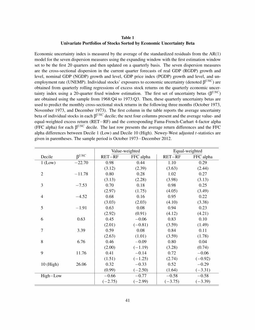
Table 1Univariate Portfolios of Stocks Sorted by Economic Uncertainty Beta

Economic uncertainty index is measured by the average of the standardized residuals from the AR(1)model for the seven dispersion measures using the expanding window with the first estimation windowset to be the first 20 quarters and then updated on a quarterly basis. The seven dispersion measuresare the cross-sectional dispersion in the current quarter forecasts of real GDP (RGDP) growth andlevel, nominal GDP (NGDP) growth and level, GDP price index (PGDP) growth and level, and un-employment rate (UNEMP). Individual stocks’ exposures to economic uncertainty (denoted βUNC) areobtained from quarterly rolling regressions of excess stock returns on the quarterly economic uncer-tainty index using a 20-quarter fixed window estimation. The first set of uncertainty betas (βUNC)are obtained using the sample from 1968:Q4 to 1973:Q3. Then, these quarterly uncertainty betas areused to predict the monthly cross-sectional stock returns in the following three months (October 1973,November 1973, and December 1973). The first column in the table reports the average uncertaintybeta of individual stocks in each βUNC decile; the next four columns present and the average value- andequal-weighted excess return (RET−RF) and the corresponding Fama-French-Carhart 4-factor alpha(FFC alpha) for each βUNC decile. The last row presents the average return differences and the FFCalpha differences between Decile 1 (Low) and Decile 10 (High). Newey-West adjusted t-statistics aregiven in parentheses. The sample period is October 1973−December 2012.

Value-weighted Equal-weightedDecile βUNC RET−RF FFC alpha RET−RF FFC alpha1 (Low) −22.70 0.98 0.44 1.10 0.29

(3.12) (2.39) (3.63) (2.44)2 −11.78 0.80 0.28 1.02 0.27

(3.13) (2.28) (3.98) (3.13)3 −7.53 0.70 0.18 0.98 0.25

(2.97) (1.75) (4.05) (3.49)4 −4.52 0.68 0.16 0.95 0.22

(3.03) (2.03) (4.10) (3.38)5 −1.91 0.63 0.08 0.94 0.23

(2.92) (0.91) (4.12) (4.21)6 0.63 0.45 −0.06 0.83 0.10

(2.01) (−0.81) (3.59) (1.49)7 3.39 0.59 0.08 0.84 0.11

(2.63) (1.01) (3.59) (1.78)8 6.76 0.46 −0.09 0.80 0.04

(2.00) (−1.19) (3.28) (0.74)9 11.76 0.41 −0.14 0.72 −0.06

(1.51) (−1.25) (2.74) (−0.92)10 (High) 26.06 0.32 −0.33 0.52 −0.29

(0.99) (−2.50) (1.64) (−3.31)High−Low −0.66 −0.77 −0.58 −0.58

(−2.75) (−2.99) (−3.75) (−3.39)

41

Table 2Portfolio Characteristics

This table reports averages of the average values of various characteristics of individual stocks in each βUNC decile, including the uncertainty beta(βUNC), market share (Mkt. shr.), stock price per share (PRC), market beta (BETA), market capitalization measured in million dollars (SIZE),book-to-market equity ratio (BM), momentum (MOM), reversal (REV), illiquidity ratio (ILLIQ), co-skewness measure (COSKEW), idiosyn-cratic volatility (IVOL), analyst forecast dispersion (DISP), firm age (AGE), and leverage (LEV). The sample period is October 1973−December2012.

Variables 1 (Low) 2 3 4 5 6 7 8 9 10 (High)βUNC −22.7 −11.78 −7.53 −4.52 −1.91 0.63 3.39 6.76 11.76 26.06Mkt. shr. 6.29% 9.63% 10.88% 11.98% 12.52% 12.84% 12.06% 10.25% 8.7% 4.85%PRC 20.29 24.52 26.35 26.76 27.26 27.44 26.46 24.96 22.68 17.94BETA 1.40 1.14 1.07 1.03 1.02 1.04 1.08 1.15 1.29 1.67SIZE 1,125 1,955 2,456 2,827 2,905 3,139 2,938 2,431 1,913 980BM 0.88 0.92 0.93 0.94 0.94 0.94 0.94 0.93 0.92 0.89MOM 33.72 21.39 18.68 17.70 17.03 16.61 16.71 17.17 18.98 32.20REV 2.69 2.00 1.77 1.69 1.68 1.63 1.71 1.72 1.87 2.53ILLIQ 1.02 0.94 0.82 0.81 0.78 0.80 0.83 0.85 0.92 1.12COSKEW −0.09 −0.08 −0.07 −0.06 −0.05 −0.04 −0.04 −0.03 −0.03 −0.02IVOL 2.45 2.04 1.88 1.80 1.79 1.80 1.86 1.95 2.14 2.60DISP 0.15 0.12 0.10 0.10 0.10 0.10 0.12 0.13 0.14 0.18AGE 201 236 249 259 266 265 260 249 227 187LEV 3.44 3.82 4.05 4.16 4.00 3.85 3.59 3.40 3.34 2.93

42

Table 3Bivariate Portfolio Sorts

In this table, stocks are first sorted into deciles based on one control variable, and then stocks within each control variable decile are furthersorted into deciles based on uncertainty beta (βUNC). The bivariate portfolios are formed based on the CRSP breakpoints. This table reports theaverage monthly returns (in percentage) for each uncertainty beta decile, averaged across the ten control groups within the same uncertainty betadecile. The control variables are market beta (BETA), log market capitalization (SIZE), log book-to-market ratio (BM), momentum (MOM),short-term reversal (REV), illiquidity (ILLIQ), co-skewness (COSKEW), idiosyncratic volatility (IVOL), analyst dispersion (DISP), firm age(AGE), and leverage (LEV). The control variables are defined in Section 2.3. The last two rows present the average return differences and theFama-French-Carhart 4-factor alpha (FFC alpha) differences between Decile 1 (Low) and Decile 10 (High). Newey-West adjusted t-statisticsare given in parentheses. The sample period is October 1973−December 2012.

Decile BETA SIZE BM MOM REV ILLIQ COSKEW IVOL DISP AGE LEVLow-βUNC 0.99 1.01 0.95 0.78 1.02 0.98 0.99 0.97 0.97 0.97 0.922 0.84 1.09 0.86 0.71 0.77 0.93 0.81 0.78 0.86 0.76 0.823 0.70 0.99 0.76 0.72 0.64 0.92 0.80 0.72 0.76 0.81 0.684 0.77 0.96 0.76 0.75 0.82 0.87 0.75 0.83 0.79 0.67 0.865 0.66 0.90 0.78 0.53 0.70 0.83 0.75 0.58 0.67 0.75 0.676 0.60 0.83 0.56 0.62 0.57 0.73 0.62 0.58 0.60 0.63 0.637 0.58 0.84 0.67 0.65 0.55 0.72 0.60 0.53 0.64 0.58 0.568 0.59 0.80 0.68 0.46 0.50 0.72 0.62 0.48 0.51 0.51 0.629 0.46 0.69 0.62 0.45 0.55 0.56 0.54 0.36 0.43 0.43 0.57High-βUNC 0.44 0.50 0.52 0.36 0.43 0.41 0.33 0.29 0.36 0.36 0.51High−Low −0.55 −0.52 −0.42 −0.42 −0.59 −0.57 −0.66 −0.68 −0.61 −0.61 −0.41

(−3.46) (−2.49) (−3.54) (−4.02) (−3.12) (−2.98) (−3.34) (−3.60) (−2.86) (−3.67) (−2.28)FFC alpha −0.48 −0.45 −0.55 −0.72 −0.65 −0.68 −0.66 −0.63 −0.70 −0.71 −0.73

(−2.91) (−2.66) (−3.16) (−4.08) (−3.29) (−3.74) (−3.44) (−3.66) (−3.50) (−3.67) (−2.83)

43

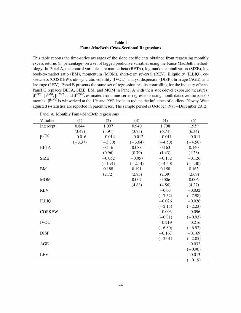
Table 4Fama-MacBeth Cross-Sectional Regressions

This table reports the time-series averages of the slope coefficients obtained from regressing monthlyexcess returns (in percentage) on a set of lagged predictive variables using the Fama-MacBeth method-ology. In Panel A, the control variables are market beta (BETA), log market capitalization (SIZE), logbook-to-market ratio (BM), momentum (MOM), short-term reversal (REV), illiquidity (ILLIQ), co-skewness (COSKEW), idiosyncratic volatility (IVOL), analyst dispersion (DISP), firm age (AGE), andleverage (LEV). Panel B presents the same set of regression results controlling for the industry effects.Panel C replaces BETA, SIZE, BM, and MOM in Panel A with their stock-level exposure measures:βMKT , βSMB, βHML, and βMOM, estimated from time-series regressions using month data over the past 60months. βUNC is winsorized at the 1% and 99% levels to reduce the influence of outliers. Newey-Westadjusted t-statistics are reported in parentheses. The sample period is October 1973−December 2012.

Panel A. Monthly Fama-MacBeth regressionsVariable (1) (2) (3) (4) (5)Intercept 0.844 1.007 0.940 1.798 1.959

(3.47) (3.91) (3.73) (6.74) (6.34)βUNC −0.016 −0.014 −0.012 −0.011 −0.011

(−3.37) (−3.80) (−3.64) (−4.50) (−4.50)BETA 0.116 0.088 0.163 0.140

(0.96) (0.79) (1.43) (1.28)SIZE −0.052 −0.057 −0.132 −0.126

(−1.91) (−2.14) (−4.50) (−4.40)BM 0.188 0.191 0.158 0.163

(2.72) (2.85) (2.39) (2.69)MOM 0.007 0.006 0.006

(4.88) (4.56) (4.27)REV −0.03 −0.032

(−7.52) (−7.98)ILLIQ −0.026 −0.026

(−2.15) (−2.23)COSKEW −0.093 −0.096

(−0.81) (−0.93)IVOL −0.219 −0.216

(−6.80) (−6.92)DISP −0.167 −0.169

(−2.01) (−2.05)AGE −0.032

(−0.90)LEV −0.013

(−0.19)

44

Table 4 – continued

Panel B. Controlling for the industry effectsVariable (1) (2) (3) (4) (5)Intercept 0.793 0.962 0.898 1.845 1.949

(3.10) (3.51) (3.33) (6.07) (6.23)βUNC −0.014 −0.013 −0.011 −0.009 −0.009

(−3.64) (−3.77) (−3.76) (−4.37) (−4.29)BETA 0.100 0.074 0.127 0.114

(0.95) (0.75) (1.30) (1.21)SIZE −0.051 −0.055 −0.130 −0.123

(−1.94) (−2.09) (−4.50) (−4.29)BM 0.219 0.219 0.217 0.184

(3.67) (3.73) (3.66) (3.36)MOM 0.006 0.005 0.005

(4.67) (4.29) (4.10)REV −0.035 −0.036

(−9.06) (−9.35)ILLIQ −0.026 −0.026

(−2.21) (−2.25)COSKEW −0.017 −0.027

(−0.19) (−0.29)IVOL −0.221 −0.219

(−7.47) (−7.54)DISP −0.185 −0.187

(−2.20) (−2.23)AGE −0.038

(−1.18)LEV 0.035

(0.63)

45

Table 4 – continued

Panel C. Using exposures to the Market, SMB, HML, and MOM factorsVariable (1) (2) (3) (4) (5)Intercept 0.844 0.726 0.686 0.930 1.503

(3.47) (4.09) (3.93) (5.59) (5.27)βUNC −0.016 −0.013 −0.013 −0.011 −0.009

(−3.37) (−3.50) (−3.35) (−4.12) (−3.75)βMKT 0.051 0.063 0.160 0.158

(0.42) (0.48) (1.11) (1.13)βSMB 0.073 0.097 0.137 0.104

(0.91) (1.15) (1.66) (1.32)βHML 0.131 0.141 0.130 0.076

(1.53) (1.62) (1.49) (1.05)βMOM −0.181 −0.16 −0.121

(−1.91) (−1.66) (−1.28)REV −0.033 −0.036

(−8.17) (−8.78)ILLIQ 0.001 −0.004

(0.06) (−0.37)COSKEW −0.2 −0.173

(−1.63) (−1.47)IVOL −0.157 −0.156

(−4.51) (−4.80)DISP −0.264 −0.247

(−2.36) (−2.33)AGE −0.116

(−2.81)LEV 0.090

(1.68)

46

Table 5Alternative Measures of Uncertainty Betas Estimated after Controlling for Market Returns and

Market Variance

In this table, individual stocks’ exposures to economic uncertainty (denoted βUNC) are obtained fromquarterly rolling regressions of excess stock returns on the quarterly economic uncertainty index aftercontrolling innovations in expected realized volatility (∆RVOL) in Model 1, ∆RVOL and excess marketreturns (Rm) in Model 2, innovations in option implied variance (∆V XO) in Model 3, and ∆V XO andRm in Model 4 using a 20-quarter fixed window estimation:

Model 1 : Ri,t = αi,t +βUNCi,t ·UNCAV G

t +βRVOLi,t ·∆VARRealized

t + εi,t ,

Model 2 : Ri,t = αi,t +βUNCi,t ·UNCAV G

t +βV XOi,t ·∆VARV XO

t + εi,t ,

Model 3 : Ri,t = αi,t +βUNCi,t ·UNCAV G

t +βRVOLi,t ·∆VARRealized

t +βMKTi,t ·Rm,t + εi,t ,

Model 4 : Ri,t = αi,t +βUNCi,t ·UNCAV G

t +βV XOi,t ·∆VARV XO

t +βMKTi,t ·Rm,t + εi,t .

These quarterly uncertainty betas are used to predict the monthly cross-sectional stock returns in thefollowing three months based on (i)univariate portfolio analysis, (ii) conditional bivariate analysis aftercontrolling for stock’s exposures to innovations in expected market variance (βRVOL estimated fromModels 1 and 2 and exposures to innovations in option implied variance (βV XO) estimated from Mod-els 3 and 4, and (iii) monthly cross-sectional Fama-MacBeth regressions. Panel A reports the averageβUNC of individual stocks within each decile sorted on βUNC and the Fama-French-Carhart 4-factoralpha (FFC alpha) for each βUNC decile and the difference between Decile 1 (Low) and Decile 10(High). Panel B reports the 4-factor alpha for each βUNC decile after controlling for exposures to inno-vations in market variance. Panel C reports the time-series averages of the slope coefficients obtainedfrom regressing monthly excess returns (in percentage) on a set of lagged predictive variables usingthe Fama-MacBeth methodology, including market beta (BETA), log market capitalization (SIZE),log book-to-market ratio (BM), momentum (MOM), short-term reversal (REV), illiquidity (ILLIQ),co-skewness (COSKEW), idiosyncratic volatility (IVOL), analyst dispersion (DISP), firm age (AGE),leverage (LEV), exposures to innovations in market variance. βUNC is winsorized at the 1% and 99%levels to reduce the influence of outliers. Newey-West adjusted t-statistics are reported in parentheses.The sample period is October 1973−December 2012.

47

Table 5 – continued

Panel A. Univariate portfolios sorted by βUNC

Decile Model (1) Model (2) Model (3) Model (4)βUNC FFC alpha βUNC FFC alpha βUNC FFC alpha βUNC FFC alpha

1 (Low) −22.96 0.40 −22.66 0.22 −29.57 0.51 −30.55 0.37(2.43) (1.45) (1.91) (1.32)

2 −11.84 0.22 −11.21 0.27 −14.46 0.33 −14.7 0.41(2.20) (2.37) (1.94) (2.14)

3 −7.52 0.22 −6.83 0.23 −8.79 0.17 −8.81 0.14(2.22) (3.07) (1.15) (1.03)

4 −4.47 0.18 −3.74 0.10 −4.82 0.19 −4.71 0.15(1.67) (1.02) (1.55) (1.19)

5 −1.8 0.01 −1.1 0.09 −1.39 0.15 −1.29 0.05(0.13) (1.16) (1.15) (0.40)

6 0.84 −0.03 1.49 −0.08 1.96 0.10 2.00 0.19(−0.51) (−1.15) (0.93) (2.21)

7 3.68 0.10 4.31 0.09 5.66 0.13 5.62 0.02(1.18) (1.18) (1.36) (0.17)

8 7.17 −0.17 7.72 −0.14 10.23 −0.11 10.05 −0.1(−2.35) (−1.77) (−1.07) (−0.92)

9 12.34 −0.18 12.90 −0.13 17.19 −0.15 16.85 −0.2(−1.50) (−1.31) (−0.93) (−1.49)

10 (High) 27.21 −0.28 27.88 −0.31 38.06 −0.38 37.58 −0.41(−2.06) (−2.37) (−2.01) (−2.07)

High−Low −0.68 −0.53 −0.89 −0.78(−2.91) (−2.46) (−2.45) (−2.19)

48

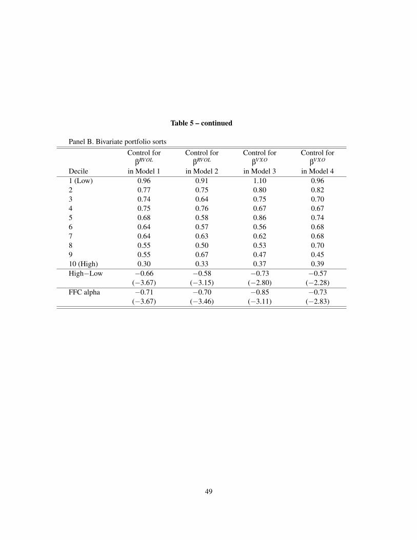
Table 5 – continued

Panel B. Bivariate portfolio sortsControl for Control for Control for Control for

βRVOL βRVOL βV XO βV XO

Decile in Model 1 in Model 2 in Model 3 in Model 41 (Low) 0.96 0.91 1.10 0.962 0.77 0.75 0.80 0.823 0.74 0.64 0.75 0.704 0.75 0.76 0.67 0.675 0.68 0.58 0.86 0.746 0.64 0.57 0.56 0.687 0.64 0.63 0.62 0.688 0.55 0.50 0.53 0.709 0.55 0.67 0.47 0.4510 (High) 0.30 0.33 0.37 0.39High−Low −0.66 −0.58 −0.73 −0.57

(−3.67) (−3.15) (−2.80) (−2.28)FFC alpha −0.71 −0.70 −0.85 −0.73

(−3.67) (−3.46) (−3.11) (−2.83)

49

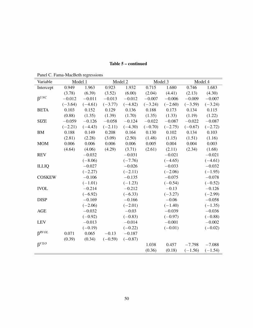
Table 5 – continued

Panel C. Fama-MacBeth regressionsVariable Model 1 Model 2 Model 3 Model 4Intercept 0.949 1.963 0.923 1.932 0.715 1.680 0.746 1.683

(3.78) (6.39) (3.52) (6.00) (2.04) (4.41) (2.13) (4.30)βUNC −0.012 −0.011 −0.013 −0.012 −0.007 −0.006 −0.009 −0.007

(−3.64) (−4.61) (−3.77) (−4.82) (−3.24) (−2.60) (−3.59) (−3.24)BETA 0.103 0.152 0.129 0.136 0.188 0.173 0.134 0.115

(0.88) (1.35) (1.39) (1.70) (1.35) (1.33) (1.19) (1.22)SIZE −0.059 −0.126 −0.058 −0.124 −0.022 −0.087 −0.022 −0.087

(−2.21) (−4.43) (−2.11) (−4.30) (−0.70) (−2.75) (−0.67) (−2.72)BM 0.188 0.149 0.208 0.164 0.130 0.102 0.134 0.103

(2.81) (2.28) (3.09) (2.50) (1.48) (1.15) (1.51) (1.16)MOM 0.006 0.006 0.006 0.006 0.005 0.004 0.004 0.003

(4.64) (4.06) (4.29) (3.71) (2.61) (2.11) (2.34) (1.68)REV −0.032 −0.031 −0.021 −0.021

(−8.06) (−7.76) (−4.65) (−4.61)ILLIQ −0.027 −0.026 −0.033 −0.032

(−2.27) (−2.11) (−2.06) (−1.95)COSKEW −0.106 −0.135 −0.075 −0.078

(−1.01) (−1.23) (−0.54) (−0.52)IVOL −0.214 −0.212 −0.13 −0.126

(−6.92) (−6.33) (−3.27) (−2.99)DISP −0.169 −0.166 −0.06 −0.058

(−2.06) (−2.01) (−1.40) (−1.35)AGE −0.032 −0.03 −0.039 −0.036

(−0.92) (−0.83) (−0.97) (−0.88)LEV −0.013 −0.014 −0.001 −0.002

(−0.19) (−0.22) (−0.01) (−0.02)βRVOL 0.071 0.065 −0.13 −0.187

(0.39) (0.34) (−0.59) (−0.87)βV XO 1.038 0.457 −7.798 −7.088

(0.36) (0.18) (−1.56) (−1.54)

50

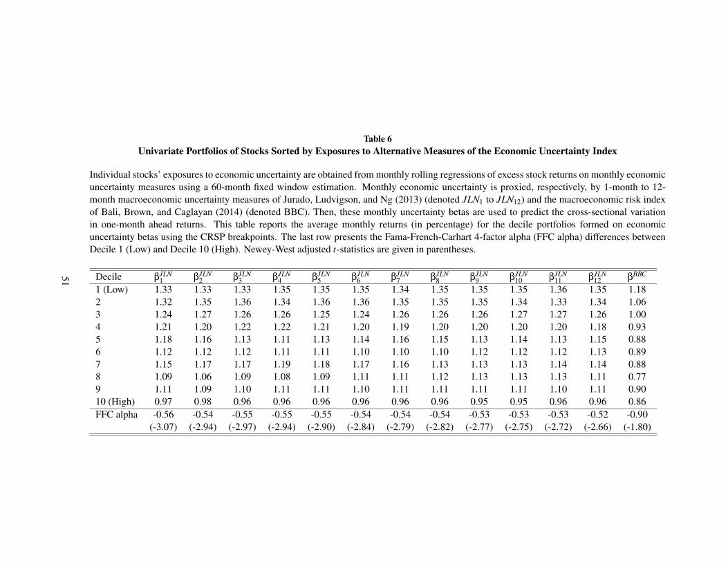
Table 6Univariate Portfolios of Stocks Sorted by Exposures to Alternative Measures of the Economic Uncertainty Index

Individual stocks’ exposures to economic uncertainty are obtained from monthly rolling regressions of excess stock returns on monthly economicuncertainty measures using a 60-month fixed window estimation. Monthly economic uncertainty is proxied, respectively, by 1-month to 12-month macroeconomic uncertainty measures of Jurado, Ludvigson, and Ng (2013) (denoted JLN1 to JLN12) and the macroeconomic risk indexof Bali, Brown, and Caglayan (2014) (denoted BBC). Then, these monthly uncertainty betas are used to predict the cross-sectional variationin one-month ahead returns. This table reports the average monthly returns (in percentage) for the decile portfolios formed on economicuncertainty betas using the CRSP breakpoints. The last row presents the Fama-French-Carhart 4-factor alpha (FFC alpha) differences betweenDecile 1 (Low) and Decile 10 (High). Newey-West adjusted t-statistics are given in parentheses.

Decile βJLN1 βJLN

2 βJLN3 βJLN

4 βJLN5 βJLN

6 βJLN7 βJLN

8 βJLN9 βJLN

10 βJLN11 βJLN

12 βBBC

1 (Low) 1.33 1.33 1.33 1.35 1.35 1.35 1.34 1.35 1.35 1.35 1.36 1.35 1.182 1.32 1.35 1.36 1.34 1.36 1.36 1.35 1.35 1.35 1.34 1.33 1.34 1.063 1.24 1.27 1.26 1.26 1.25 1.24 1.26 1.26 1.26 1.27 1.27 1.26 1.004 1.21 1.20 1.22 1.22 1.21 1.20 1.19 1.20 1.20 1.20 1.20 1.18 0.935 1.18 1.16 1.13 1.11 1.13 1.14 1.16 1.15 1.13 1.14 1.13 1.15 0.886 1.12 1.12 1.12 1.11 1.11 1.10 1.10 1.10 1.12 1.12 1.12 1.13 0.897 1.15 1.17 1.17 1.19 1.18 1.17 1.16 1.13 1.13 1.13 1.14 1.14 0.888 1.09 1.06 1.09 1.08 1.09 1.11 1.11 1.12 1.13 1.13 1.13 1.11 0.779 1.11 1.09 1.10 1.11 1.11 1.10 1.11 1.11 1.11 1.11 1.10 1.11 0.9010 (High) 0.97 0.98 0.96 0.96 0.96 0.96 0.96 0.96 0.95 0.95 0.96 0.96 0.86FFC alpha -0.56 -0.54 -0.55 -0.55 -0.55 -0.54 -0.54 -0.54 -0.53 -0.53 -0.53 -0.52 -0.90

(-3.07) (-2.94) (-2.97) (-2.94) (-2.90) (-2.84) (-2.79) (-2.82) (-2.77) (-2.75) (-2.72) (-2.66) (-1.80)

51

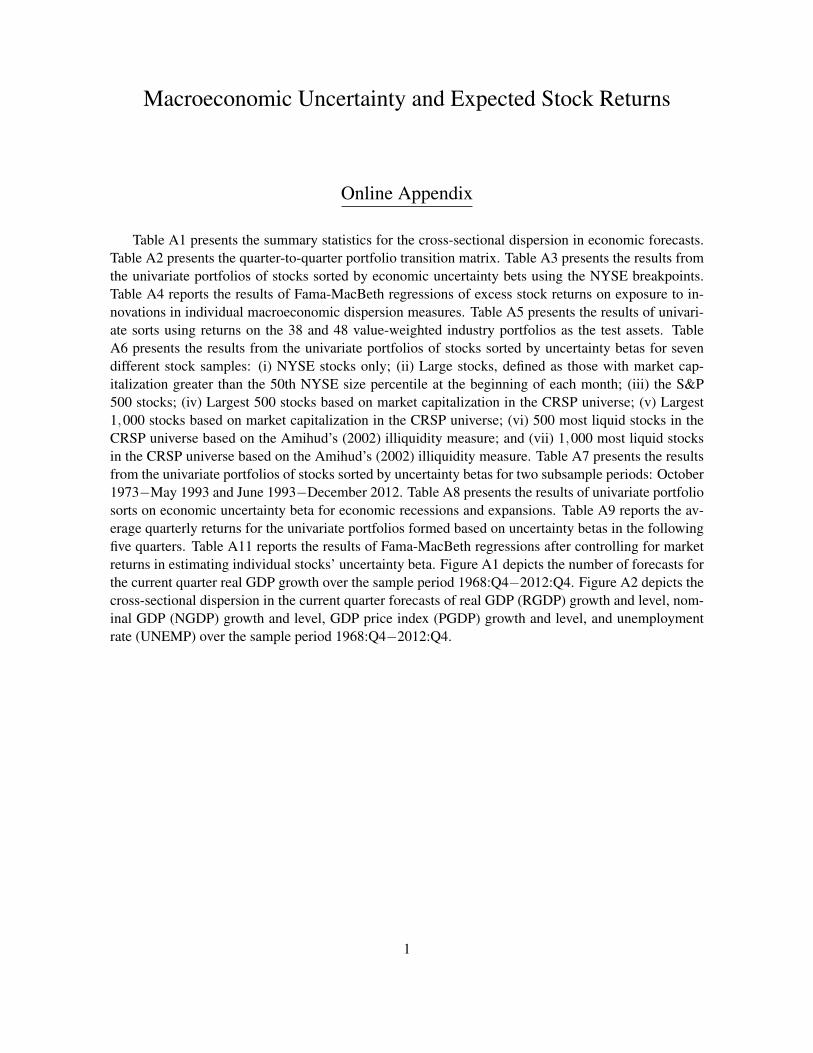
Macroeconomic Uncertainty and Expected Stock Returns

Online Appendix

Table A1 presents the summary statistics for the cross-sectional dispersion in economic forecasts.Table A2 presents the quarter-to-quarter portfolio transition matrix. Table A3 presents the results fromthe univariate portfolios of stocks sorted by economic uncertainty bets using the NYSE breakpoints.Table A4 reports the results of Fama-MacBeth regressions of excess stock returns on exposure to in-novations in individual macroeconomic dispersion measures. Table A5 presents the results of univari-ate sorts using returns on the 38 and 48 value-weighted industry portfolios as the test assets. TableA6 presents the results from the univariate portfolios of stocks sorted by uncertainty betas for sevendifferent stock samples: (i) NYSE stocks only; (ii) Large stocks, defined as those with market cap-italization greater than the 50th NYSE size percentile at the beginning of each month; (iii) the S&P500 stocks; (iv) Largest 500 stocks based on market capitalization in the CRSP universe; (v) Largest1,000 stocks based on market capitalization in the CRSP universe; (vi) 500 most liquid stocks in theCRSP universe based on the Amihud’s (2002) illiquidity measure; and (vii) 1,000 most liquid stocksin the CRSP universe based on the Amihud’s (2002) illiquidity measure. Table A7 presents the resultsfrom the univariate portfolios of stocks sorted by uncertainty betas for two subsample periods: October1973−May 1993 and June 1993−December 2012. Table A8 presents the results of univariate portfoliosorts on economic uncertainty beta for economic recessions and expansions. Table A9 reports the av-erage quarterly returns for the univariate portfolios formed based on uncertainty betas in the followingfive quarters. Table A11 reports the results of Fama-MacBeth regressions after controlling for marketreturns in estimating individual stocks’ uncertainty beta. Figure A1 depicts the number of forecasts forthe current quarter real GDP growth over the sample period 1968:Q4−2012:Q4. Figure A2 depicts thecross-sectional dispersion in the current quarter forecasts of real GDP (RGDP) growth and level, nom-inal GDP (NGDP) growth and level, GDP price index (PGDP) growth and level, and unemploymentrate (UNEMP) over the sample period 1968:Q4−2012:Q4.

1

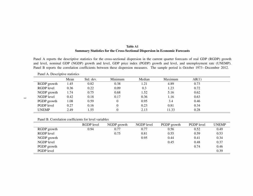
Table A1Summary Statistics for the Cross-Sectional Dispersion in Economic Forecasts

Panel A reports the descriptive statistics for the cross-sectional dispersion in the current quarter forecasts of real GDP (RGDP) growthand level, nominal GDP (NGDP) growth and level, GDP price index (PGDP) growth and level, and unemployment rate (UNEMP).Panel B reports the correlation coefficients between these dispersion measures. The sample period is October 1973−December 2012.

Panel A. Descriptive statisticsMean Std. dev. Minimum Median Maximum AR(1)

RGDP growth 1.45 0.82 0.38 1.21 4.89 0.73RGDP level 0.36 0.22 0.09 0.3 1.23 0.72NGDP growth 1.74 0.75 0.68 1.52 5.16 0.62NGDP level 0.42 0.18 0.17 0.36 1.16 0.63PGDP growth 1.08 0.59 0 0.95 3.4 0.46PGDP level 0.27 0.16 0 0.23 0.81 0.34UNEMP 2.49 1.55 0 2.13 11.33 0.28

Panel B. Correlation coefficients for level variablesRGDP level NGDP growth NGDP level PGDP growth PGDP level UNEMP

RGDP growth 0.94 0.77 0.77 0.56 0.52 0.49RGDP level 0.75 0.81 0.55 0.59 0.53NGDP growth 0.95 0.44 0.41 0.34NGDP level 0.45 0.48 0.37PGDP growth 0.74 0.46PGDP level 0.39

1

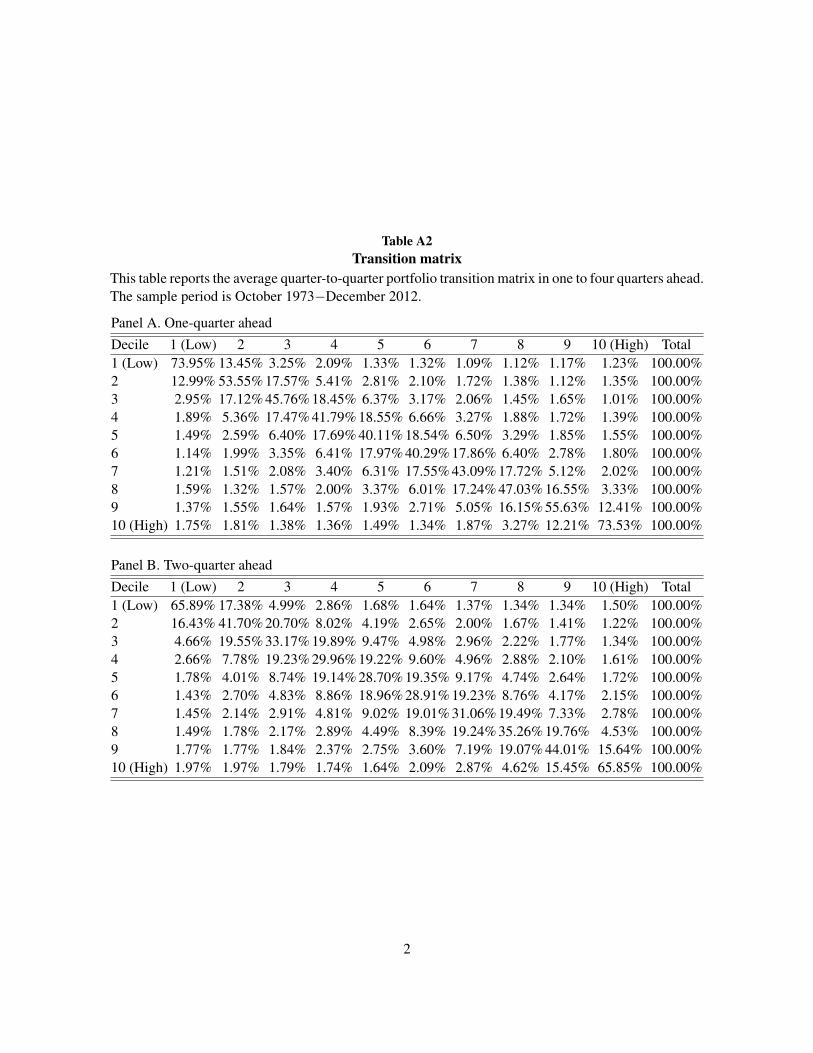
Table A2Transition matrix

This table reports the average quarter-to-quarter portfolio transition matrix in one to four quarters ahead.The sample period is October 1973−December 2012.

Panel A. One-quarter aheadDecile 1 (Low) 2 3 4 5 6 7 8 9 10 (High) Total1 (Low) 73.95% 13.45% 3.25% 2.09% 1.33% 1.32% 1.09% 1.12% 1.17% 1.23% 100.00%2 12.99% 53.55% 17.57% 5.41% 2.81% 2.10% 1.72% 1.38% 1.12% 1.35% 100.00%3 2.95% 17.12% 45.76% 18.45% 6.37% 3.17% 2.06% 1.45% 1.65% 1.01% 100.00%4 1.89% 5.36% 17.47% 41.79% 18.55% 6.66% 3.27% 1.88% 1.72% 1.39% 100.00%5 1.49% 2.59% 6.40% 17.69% 40.11% 18.54% 6.50% 3.29% 1.85% 1.55% 100.00%6 1.14% 1.99% 3.35% 6.41% 17.97% 40.29% 17.86% 6.40% 2.78% 1.80% 100.00%7 1.21% 1.51% 2.08% 3.40% 6.31% 17.55% 43.09% 17.72% 5.12% 2.02% 100.00%8 1.59% 1.32% 1.57% 2.00% 3.37% 6.01% 17.24% 47.03% 16.55% 3.33% 100.00%9 1.37% 1.55% 1.64% 1.57% 1.93% 2.71% 5.05% 16.15% 55.63% 12.41% 100.00%10 (High) 1.75% 1.81% 1.38% 1.36% 1.49% 1.34% 1.87% 3.27% 12.21% 73.53% 100.00%

Panel B. Two-quarter aheadDecile 1 (Low) 2 3 4 5 6 7 8 9 10 (High) Total1 (Low) 65.89% 17.38% 4.99% 2.86% 1.68% 1.64% 1.37% 1.34% 1.34% 1.50% 100.00%2 16.43% 41.70% 20.70% 8.02% 4.19% 2.65% 2.00% 1.67% 1.41% 1.22% 100.00%3 4.66% 19.55% 33.17% 19.89% 9.47% 4.98% 2.96% 2.22% 1.77% 1.34% 100.00%4 2.66% 7.78% 19.23% 29.96% 19.22% 9.60% 4.96% 2.88% 2.10% 1.61% 100.00%5 1.78% 4.01% 8.74% 19.14% 28.70% 19.35% 9.17% 4.74% 2.64% 1.72% 100.00%6 1.43% 2.70% 4.83% 8.86% 18.96% 28.91% 19.23% 8.76% 4.17% 2.15% 100.00%7 1.45% 2.14% 2.91% 4.81% 9.02% 19.01% 31.06% 19.49% 7.33% 2.78% 100.00%8 1.49% 1.78% 2.17% 2.89% 4.49% 8.39% 19.24% 35.26% 19.76% 4.53% 100.00%9 1.77% 1.77% 1.84% 2.37% 2.75% 3.60% 7.19% 19.07% 44.01% 15.64% 100.00%10 (High) 1.97% 1.97% 1.79% 1.74% 1.64% 2.09% 2.87% 4.62% 15.45% 65.85% 100.00%

2

Table A2 – continued

Panel C. Three-quarter aheadDecile 1 (Low) 2 3 4 5 6 7 8 9 10 (High) Total1 (Low) 59.60% 18.96% 6.68% 3.69% 2.42% 2.01% 1.64% 1.65% 1.58% 1.75% 100.00%2 17.39% 34.74% 20.60% 9.89% 5.58% 3.63% 2.65% 2.18% 1.86% 1.48% 100.00%3 6.12% 19.26% 27.52% 19.20% 11.05% 6.23% 3.75% 2.98% 2.10% 1.79% 100.00%4 3.30% 9.65% 18.53% 24.51% 18.32% 11.00% 6.36% 3.84% 2.53% 1.96% 100.00%5 2.21% 5.21% 10.15% 18.24% 23.49% 18.16% 10.78% 6.06% 3.54% 2.17% 100.00%6 1.79% 3.35% 6.14% 10.50% 17.96% 23.98% 18.36% 10.08% 5.38% 2.46% 100.00%7 1.64% 2.59% 3.82% 6.20% 10.33% 18.21% 25.71% 19.02% 9.05% 3.43% 100.00%8 1.66% 2.16% 2.91% 3.74% 5.95% 9.84% 18.99% 29.10% 20.00% 5.65% 100.00%9 2.08% 1.99% 2.21% 2.76% 3.50% 4.92% 8.79% 19.74% 37.19% 16.84% 100.00%10 (High) 2.24% 2.56% 2.02% 2.10% 2.18% 2.75% 3.79% 5.90% 16.90% 59.55% 100.00%

Panel D. Four-quarter aheadDecile 1 (Low) 2 3 4 5 6 7 8 9 10 (High) Total1 (Low) 54.03% 19.66% 8.21% 4.65% 3.15% 2.42% 2.00% 1.92% 1.88% 2.08% 100.00%2 17.53% 29.72% 19.81% 11.23% 6.76% 4.40% 3.53% 2.72% 2.36% 1.96% 100.00%3 7.36% 18.44% 23.52% 18.32% 11.88% 7.26% 4.71% 3.66% 2.74% 2.10% 100.00%4 3.96% 10.49% 17.60% 21.24% 17.25% 11.69% 7.48% 4.85% 3.25% 2.20% 100.00%5 2.72% 6.59% 11.06% 16.58% 20.12% 17.40% 11.41% 7.02% 4.34% 2.76% 100.00%6 2.12% 4.22% 7.18% 11.45% 16.90% 20.55% 17.58% 10.95% 6.09% 2.98% 100.00%7 2.09% 3.11% 4.94% 7.30% 11.07% 16.91% 22.08% 18.19% 10.08% 4.23% 100.00%8 1.93% 2.84% 3.48% 4.47% 7.07% 11.20% 17.94% 25.13% 19.31% 6.63% 100.00%9 2.42% 2.27% 2.62% 3.50% 4.17% 6.13% 10.05% 19.25% 32.39% 17.21% 100.00%10 (High) 2.71% 2.59% 2.51% 2.44% 2.68% 3.26% 4.32% 7.05% 17.76% 54.68% 100.00%

3

Table A3Univariate Portfolios of Stocks Sorted by Economic Uncertainty Betas using the NYSE

Breakpoints

In this table, individual stocks’ exposures to economic uncertainty (denoted βUNC) are obtainedfrom quarterly rolling regressions of excess stock returns on the quarterly economic uncer-tainty index using a 20-quarter fixed window estimation. The first set of uncertainty betas(βUNC) are obtained using the sample from 1968:Q4 to 1973:Q3. Then, these quarterly un-certainty betas are used to predict the monthly cross-sectional stock returns in the followingthree months (October 1973, November 1973, and December 1973). This table reports thevalue-weighted and equal-weighted monthly returns (in percentage) and the Fama-French-Carhart4-factor alpha for the decile portfolios formed on βUNC using the NYSE breakpoints. The lasttwo rows present the average return differences and the Fama-French-Carhart 4-factor alpha(FFC alpha) differences between Decile 1 (Low) and Decile 10 (High). Newey-West adjustedt-statistics are given in parentheses. The sample period is October 1973−December 2012.

Value-weighted Equal-weightedDecile RET−RF FFC4 alpha RET−RF FFC4 alpha1 (Low) 0.91 0.39 1.10 0.30

(3.00) (2.25) (3.73) (2.62)2 0.81 0.27 0.98 0.23

(3.43) (2.67) (3.88) (2.61)3 0.67 0.10 0.99 0.26

(2.85) (1.16) (4.10) (3.64)4 0.71 0.22 0.95 0.24

(3.19) (2.44) (4.15) (3.71)5 0.56 0.00 0.90 0.19

(2.60) (−0.04) (3.96) (3.33)6 0.43 −0.06 0.83 0.12

(1.96) (−0.80) (3.63) (1.67)7 0.61 0.13 0.89 0.16

(2.79) (1.61) (3.80) (2.68)8 0.46 −0.07 0.80 0.05

(1.96) (−0.90) (3.29) (0.75)9 0.49 −0.07 0.78 0.01

(2.00) (−0.67) (3.07) (0.17)10 (High) 0.37 −0.26 0.59 −0.21

(1.22) (−2.32) (1.96) (−2.91)High−Low −0.54 −0.65 −0.51 −0.51

(−2.40) (−2.76) (−3.81) (−3.37)

4

Table A4Fama-MacBeth Cross-Sectional Regressions

Economic uncertainty index is measured by the standardized residuals from the AR(1) model for adispersion measure using the expanding window with the first estimation window set to be the first20 quarters and then updated on a quarterly basis. The seven dispersion measures are the cross-sectional dispersion in the current quarter forecasts of real GDP (RGDP) growth and level, nomi-nal GDP (NGDP) growth and level, GDP price index (PGDP) growth and level, and unemploymentrate (UNEMP). The Individual stocks’ exposures to economic uncertainty (denoted βUNC) are ob-tained from quarterly rolling regressions of excess stock returns on the quarterly economic uncer-tainty index using a 20-quarter fixed window estimation. These quarterly uncertainty betas are usedto predict the monthly cross-sectional stock returns in the following three months after controllingfor a large set of stock return predictors after controlling for a large set of stock return predictors,including market beta (BETA), log market capitalization (SIZE), log book-to-market ratio (BM), mo-mentum (MOM), short-term reversal (REV), illiquidity (ILLIQ), co-skewness (COSKEW), idiosyn-cratic volatility (IVOL), analyst dispersion (DISP), firm age (AGE), and leverage (LEV). This tablereports the time-series averages of the slope coefficients obtained from regressing monthly excess re-turns (in percentage) on a set of lagged predictive variables using the Fama-MacBeth methodology.βUNC is winsorized at the 1% and 99% levels to reduce the influence of outliers. Newey-West ad-justed t-statistics are reported in parentheses. The sample period is October 1973−December 2012.

RGDP NGDP PGDP UNEMPVariable Growth Level Growth Level Growth LevelIntercept 1.953 1.938 1.959 1.947 1.975 1.975 1.992

(6.32) (6.28) (6.29) (6.25) (6.29) (6.27) (6.38)βUNC -0.011 -0.003 -0.008 -0.002 -0.002 -0.001 -0.013

(-3.55) (-3.28) (-3.38) (-2.60) (-1.94) (-1.85) (-1.90)BETA 0.125 0.126 0.148 0.145 0.126 0.126 0.141

(1.15) (1.16) (1.32) (1.31) (1.17) (1.15) (1.28)LNME -0.124 -0.124 -0.124 -0.124 -0.120 -0.122 -0.127

(-4.28) (-4.30) (-4.27) (-4.30) (-4.15) (-4.22) (-4.36)LNBM 0.159 0.171 0.161 0.159 0.160 0.162 0.166

(2.62) (2.82) (2.68) (2.63) (2.67) (2.68) (2.74)MOM 0.006 0.006 0.006 0.006 0.006 0.006 0.006

(4.49) (4.45) (4.41) (4.39) (4.03) (3.97) (4.13)REV -0.032 -0.032 -0.031 -0.032 -0.032 -0.032 -0.032

(-7.92) (-7.89) (-7.98) (-7.98) (-8.02) (-8.09) (-7.98)ILLIQ -0.027 -0.027 -0.026 -0.027 -0.027 -0.027 -0.028

(-2.29) (-2.25) (-2.23) (-2.24) (-2.30) (-2.32) (-2.34)COSKEW -0.127 -0.091 -0.113 -0.107 -0.121 -0.104 -0.151

(-1.24) (-0.87) (-1.06) (-1.00) (-1.21) (-1.02) (-1.42)IVOL -0.215 -0.216 -0.217 -0.217 -0.218 -0.218 -0.216

(-6.93) (-6.93) (-6.96) (-6.96) (-7.04) (-7.04) (-6.98)DISP -0.171 -0.167 -0.171 -0.171 -0.170 -0.168 -0.168

(-2.06) (-2.03) (-2.08) (-2.09) (-2.05) (-2.09) (-2.07)LNAGE -0.031 -0.030 -0.033 -0.031 -0.036 -0.035 -0.034

(-0.89) (-0.86) (-0.93) (-0.89) (-1.01) (-0.97) (-0.96)LNAM -0.004 -0.008 -0.009 -0.007 -0.012 -0.011 -0.009

(-0.07) (-0.12) (-0.13) (-0.10) (-0.18) (-0.16) (-0.14)5

Table A5Univariate Portfolios Using Industry Portfolios as Test Assets

In this table, individual industries’ exposures to economic uncertainty (denoted βUNC) are ob-tained from quarterly rolling regressions of excess returns for the 38 and 48 Fama-French value-weighted industry portfolios on the quarterly economic uncertainty index using a 20-quarter fixedwindow estimation. The first set of uncertainty betas (βUNC) are obtained using the sample from1968:Q4 to 1973:Q3. Then, these quarterly uncertainty betas are used to predict the monthly cross-sectional stock returns in the following three months (October 1973, November 1973, and Decem-ber 1973). This table reports the average uncertainty beta (βUNC), average monthly returns (in per-centage), and the Fama-French-Carhart 4-factor alpha for the decile portfolios formed on βUNC.The last two rows present the average return differences and the Fama-French-Carhart 4-factor al-pha (FFC alpha) differences between Decile 1 (Low) and Decile 10 (High). Newey-West ad-justed t-statistics are given in parentheses. The sample period is October 1973−December 2012.

38 industries 48 industriesDecile βUNC RET−RF FFC alpha βUNC RET−RF FFC alpha1 (Low) −8.25 1.06 0.44 −8.89 1.10 0.41

(3.83) (2.35) (4.28) (2.47)2 −4.73 0.69 0.09 −4.73 0.67 0.04

(2.70) (0.65) (2.76) (0.30)3 −3.22 0.66 0.01 −3.08 0.71 0.01

(2.55) (0.05) (2.73) (0.10)4 −2.12 0.76 0.12 −1.76 0.63 0.04

(3.25) (1.00) (2.55) (0.41)5 −0.95 0.62 0.04 −0.65 0.68 0.01

(2.35) (0.39) (2.51) (0.09)6 0.12 0.56 −0.06 0.39 0.65 0.03

(2.02) (−0.61) (2.63) (0.37)7 1.13 0.58 0.01 1.69 0.60 0.00

(2.34) (0.04) (2.33) (−0.01)8 2.37 0.60 0.02 3.14 0.56 −0.05

(2.68) (0.15) (2.31) (−0.47)9 3.90 0.53 −0.06 4.85 0.52 −0.13

(2.13) (−0.52) (1.96) (−1.06)10 (High) 7.35 0.52 −0.22 8.77 0.46 −0.29

(1.76) (−1.36) (1.60) (−1.96)High−Low −0.54 −0.67 −0.63 −0.70

(−1.99) (−2.31) (−2.90) (−2.92)

6

Table A6Different Stock Samples

In this table, individual stocks’ exposures to economic uncertainty (denoted βUNC) are obtained from quarterly rolling regressions of excessstock returns on the quarterly economic uncertainty index using a 20-quarter fixed window estimation. These quarterly uncertainty betas areused to predict the monthly cross-sectional stock returns in the following three months. Sensitivity of our main findings is tested for sevendifferent stock samples: (i) NYSE stocks only; (ii) Large stocks, defined as those with market capitalization greater than the 50th NYSEsize percentile at the beginning of each month; (iii) the S&P 500 stocks; (iv) Largest 500 stocks based on market capitalization in the CRSPuniverse; (v) Largest 1,000 stocks based on market capitalization in the CRSP universe; (vi) 500 most liquid stocks in the CRSP universe basedon the Amihud’s (2002) illiquidity measure; and (vii) 1,000 most liquid stocks in the CRSP universe based on the Amihud’s (2002) illiquiditymeasure. This table reports the average monthly returns (in percentage) for the decile portfolios formed on βUNC using the CRSP breakpoints.The last two rows present the average return differences and the Fama-French-Carhart 4-factor alpha (FFC alpha) differences between Decile 1(Low) and Decile 10 (High). Newey-West adjusted t-statistics are given in parentheses. The sample period is October 1973−December 2012.

Decile NYSE Large S&P500 500 largest 1,000 largest 500 most liquid 1,000 most liquid1 (Low) 0.29 0.37 0.45 0.34 0.36 0.40 0.41

(1.66) (2.32) (2.62) (2.19) (2.31) (2.52) (2.41)2 0.16 0.18 0.18 0.27 0.22 0.29 0.25

(1.43) (1.79) (1.86) (2.44) (2.28) (2.53) (2.39)3 0.10 0.23 0.27 0.19 0.22 0.24 0.23

(0.99) (2.46) (2.65) (1.98) (2.45) (2.58) (2.40)4 0.14 0.16 0.11 0.12 0.18 0.09 0.20

(1.58) (1.76) (1.06) (1.21) (1.94) (0.96) (2.19)5 0.00 −0.01 0.00 0.02 0.00 −0.02 −0.01

(−0.02) (−0.21) (0.01) (0.30) (−0.01) (−0.29) (−0.11)6 −0.11 −0.05 −0.02 −0.06 0.01 −0.04 0.01

(−1.51) (−0.61) (−0.23) (−0.68) (0.19) (−0.42) (0.07)7 0.09 0.05 −0.03 0.01 −0.06 0.00 −0.04

(1.02) (0.77) (−0.37) (0.18) (−0.73) (−0.01) (−0.55)8 −0.05 −0.09 −0.06 −0.12 −0.02 −0.14 −0.05

(−0.62) (−0.95) (−0.52) (−1.32) (−0.26) (−1.45) (−0.59)9 −0.16 −0.15 −0.01 −0.14 −0.13 −0.1 −0.11

(−1.66) (−1.37) (−0.07) (−1.29) (−1.17) (−0.90) (−0.98)10 (High) −0.22 −0.15 −0.14 −0.13 −0.23 −0.17 −0.21

(−1.81) (−1.27) (−1.07) (−1.03) (−1.97) (−1.38) (−1.78)High−Low −0.51 −0.52 −0.59 −0.47 −0.59 −0.56 −0.62

(−2.35) (−2.30) (−2.26) (−2.04) (−2.69) (−2.53) (−2.73)

7

Table A7Subsample Analysis

In this table, individual stocks’ exposures to economic uncertainty (denoted βUNC) are obtained fromquarterly rolling regressions of excess stock returns on the quarterly economic uncertainty index us-ing a 20-quarter fixed window estimation. These quarterly uncertainty betas are used to predict themonthly cross-sectional stock returns in the following three months. This table reports the averagemonthly returns (in percentage) for the decile portfolios formed on βUNC for two subsample peri-ods: October 1973−May 1993 and June 1993−December 2012. The last two rows present the aver-age return differences and the Fama-French-Carhart 4-factor alpha (FFC alpha) differences betweenDecile 1 (Low) and Decile 10 (High). Newey-West adjusted t-statistics are given in parentheses.

Decile Oct 1973−May 1993 June 1993−Dec 20121 (Low) 0.19 0.57

(1.40) (1.86)2 0.29 0.25

(2.87) (1.25)3 0.21 0.18

(2.16) (1.10)4 0.14 0.22

(1.69) (1.80)5 −0.03 0.23

(−0.25) (1.76)6 −0.12 0.02

(−1.46) (0.19)7 0.03 0.14

(0.24) (1.40)8 −0.05 −0.11

(−0.55) (−1.12)9 −0.2 −0.16

(−1.48) (−0.93)10 (High) −0.38 −0.41

(−2.41) (−1.98)High−Low −0.58 −0.97

(−2.45) (−2.34)

8

Table A8Univariate portfolio analysis for economic recessions and expansions

In this table, individual stocks’ exposures to economic uncertainty (denoted βUNC) are ob-tained from quarterly rolling regressions of excess stock returns on the quarterly economic un-certainty index using a 20-quarter fixed window estimation. These quarterly uncertainty be-tas are used to predict the monthly cross-sectional stock returns in the following three months.This table reports the Fama-French-Carhart 4-factor alpha (in percentage) for the decile portfo-lios formed on βUNC and the 4-factor alpha (FFC alpha) differences between Decile 1 (Low) andDecile 10 (High) for economic recessions and expansions. Monthly observations over the pe-riod October 1973−December 2012 are divided into the normal (bad) state in which the three-month moving average of the Chicago Fed National Activity Index (CFNAIMA3) is above (be-low) −0.7 or the U.S. economy in expansion (recession) as marked by the National Bureauof Economic Research (NBER). Newey-West adjusted t-statistics are given in parentheses.

Decile Recession−NBER Expansion−NBER Recession−CFNAI Recession−CFNAI1 (Low) 0.85 0.34 0.93 0.35

(1.95) (1.86) (1.77) (2.01)2 0.63 0.24 0.46 0.26

(2.95) (1.76) (1.60) (1.92)3 0.80 0.04 0.87 0.06

(3.52) (0.41) (3.31) (0.59)4 0.36 0.15 0.28 0.10

(2.11) (1.62) (1.67) (1.14)5 −0.01 0.08 0.08 0.07

(−0.05) (0.86) (0.45) (0.79)6 −0.21 −0.03 −0.13 −0.04

(−0.87) (−0.42) (−0.67) (−0.55)7 −0.11 0.12 0.07 0.11

(−0.47) (1.64) (0.34) (1.55)8 −0.2 −0.08 −0.09 −0.07

(−1.00) (−1.14) (−0.47) (−0.94)9 −0.64 −0.09 −0.87 −0.02

(−1.85) (−0.77) (−3.45) (−0.20)10 (High) −0.95 −0.28 −0.93 −0.22

(−3.51) (−1.86) (−3.13) (−1.46)High−Low −1.8 −0.62 −1.86 −0.57

(−3.44) (−2.26) (−2.98) (−2.08)

9

Table A9Long-term Predictive Power of Economic Uncertainty Betas

In this table, individual stocks’ exposures to economic uncertainty (denoted βUNC) are obtainedfrom quarterly rolling regressions of excess stock returns on the quarterly economic uncertainty in-dex using a 20-quarter fixed window estimation. These quarterly uncertainty betas are used topredict the quarterly cross-sectional stock returns in the following one to five quarters ahead (i.e.,quarters 1−5). This table reports the Fama-French-Carhart 4-factor alpha (in percentage) of thequarterly returns for the decile portfolios formed on βUNC as well as the 4-factor alpha (FFC al-pha) differences in quarterly returns between Decile 1 (Low) and Decile 10 (High). Newey-West adjusted t-statistics are given in parentheses. The sample period is 1973:Q4−2012:Q4.

Decile QTR1 QTR2 QTR3 QTR41 (Low) 1.60 0.73 0.67 0.60

(2.38) (1.59) (1.71) (1.68)2 0.63 1.32 0.82 0.75

(1.59) (2.27) (2.43) (2.45)3 0.43 0.38 −0.08 0.71

(1.18) (1.55) (−0.39) (2.61)4 0.47 0.25 0.56 0.51

(2.01) (0.92) (1.97) (2.15)5 0.45 0.39 0.08 0.13

(1.49) (1.41) (0.42) (0.49)6 −0.34 −0.07 −0.11 0.06

(−1.34) (−0.28) (−0.58) (0.29)7 0.12 −0.26 0.09 0.33

(0.60) (−1.11) (0.39) (1.02)8 −0.31 −0.09 0.12 0.13

(−1.57) (−0.31) (0.58) (0.41)9 −0.68 −0.71 −0.25 −0.19

(−1.88) (−2.06) (−0.78) (−0.55)10 (High) −0.48 −0.97 −0.6 −0.31

(−1.21) (−2.07) (−1.51) (−0.85)High−Low −2.08 −1.70 −1.27 −0.92

(−2.40) (−2.33) (−1.99) (−1.64)

10

Table A10Fama-MacBeth Cross-Sectional Regressions after Controlling for Market Return

In this table, individual stocks’ exposures to economic uncertainty (denoted βUNC) are obtainedfrom quarterly rolling regressions of excess stock returns on the quarterly economic uncertainty in-dex after controlling for excess quarterly market returns using a 20-quarter fixed window estima-tion. These quarterly uncertainty betas are used to predict the monthly cross-sectional stock re-turns in the following three months after controlling for a large set of stock return predictors af-ter controlling for a large set of stock return predictors, including market beta (BETA), log mar-ket capitalization (SIZE), log book-to-market ratio (BM), momentum (MOM), short-term rever-sal (REV), illiquidity (ILLIQ), co-skewness (COSKEW), idiosyncratic volatility (IVOL), analystdispersion (DISP), firm age (AGE), and leverage (LEV). This table reports the time-series av-erages of the slope coefficients obtained from regressing monthly excess returns (in percentage)on a set of lagged predictive variables using the Fama-MacBeth methodology. βUNC is win-sorized at the 1% and 99% levels to reduce the influence of outliers. Newey-West adjusted t-statistics are reported in parentheses. The sample period is October 1973−December 2012.

Variable (1) (2) (3) (4) (5) (6)Intercept 0.880 0.744 0.994 0.908 1.774 1.917

(3.60) (3.94) (3.72) (3.44) (6.56) (5.93)βUNC −0.012 −0.017 −0.016 −0.014 −0.013 −0.012

(−3.14) (−3.89) (−4.07) (−3.76) (−4.77) (−4.76)BETA 0.125 0.155 0.129 0.162 0.144

(1.18) (1.60) (1.43) (1.95) (1.84)SIZE −0.052 −0.056 −0.129 −0.123

(−1.83) (−2.02) (−4.31) (−4.26)BM 0.209 0.209 0.174 0.180

(2.93) (3.06) (2.60) (2.89)MOM 0.006 0.006 0.006

(4.43) (4.21) (3.83)REV −0.029 −0.030

(−7.15) (−7.64)ILLIQ −0.025 −0.025

(−1.98) (−2.06)COSKEW −0.122 −0.122

(−1.02) (−1.11)IVOL −0.218 −0.214

(−6.24) (−6.33)DISP −0.164 −0.166

(−1.95) (−1.99)AGE −0.028

(−0.78)LEV −0.014

(−0.21)

11

Table A11Fama-MacBeth Cross-Sectional Regressions with beta on UNCPCA

Economic uncertainty index is measured by the first principal component of the standardized residualsfrom the AR(1) model for the seven dispersion measures using the expanding window with the firstestimation window set to be the first 20 quarters and then updated on a quarterly basis. The Individualstocks’ exposures to economic uncertainty (denoted βUNC) are obtained from quarterly rolling regres-sions of excess stock returns on the quarterly economic uncertainty index after controlling for excessquarterly market returns using a 20-quarter fixed window estimation. These quarterly uncertainty be-tas are used to predict the monthly cross-sectional stock returns in the following three months aftercontrolling for a large set of stock return predictors after controlling for a large set of stock returnpredictors, including market beta (BETA), log market capitalization (SIZE), log book-to-market ratio(BM), momentum (MOM), short-term reversal (REV), illiquidity (ILLIQ), co-skewness (COSKEW),idiosyncratic volatility (IVOL), analyst dispersion (DISP), firm age (AGE), and leverage (LEV). Thistable reports the time-series averages of the slope coefficients obtained from regressing monthly excessreturns (in percentage) on a set of lagged predictive variables using the Fama-MacBeth methodology.βUNC is winsorized at the 1% and 99% levels to reduce the influence of outliers. Newey-West ad-justed t-statistics are reported in parentheses. The sample period is October 1973−December 2012.

Variable (1) (2) (3) (4) (5)Intercept 0.849 1.001 0.936 1.796 1.955

(3.48) (3.87) (3.70) (6.71) (6.33)βUNC −0.041 −0.037 −0.033 −0.032 −0.032

(−3.21) (−3.60) (−3.55) (−4.45) (−4.45)BETA 0.122 0.093 0.164 0.142

(1.01) (0.82) (1.45) (1.29)LNME −0.052 −0.057 −0.132 −0.126

(−1.89) (−2.11) (−4.49) (−4.38)LNBM 0.192 0.193 0.159 0.163

(2.77) (2.88) (2.39) (2.68)MOM 0.007 0.006 0.006

(4.90) (4.63) (4.35)REV −0.030 −0.032

(−7.50) (−7.96)ILLIQ −0.026 −0.026

(−2.15) (−2.23)COSKEW −0.090 −0.094

(−0.77) (−0.90)IVOL −0.219 −0.215

(−6.80) (−6.91)DISP −0.168 −0.170

(−2.02) (−2.05)AGE −0.031

(−0.89)LEV −0.011

(−0.17)

12

Figure A1. Number of Forecasts This figure depicts the number of forecasts for the current quarterreal GDP growth over the sample period 1968:Q4−2012:Q4.

13

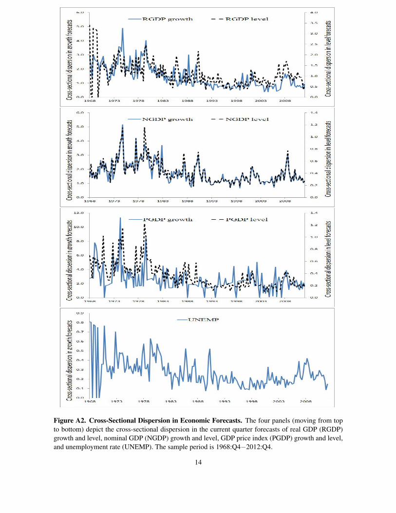
Figure A2. Cross-Sectional Dispersion in Economic Forecasts. The four panels (moving from topto bottom) depict the cross-sectional dispersion in the current quarter forecasts of real GDP (RGDP)growth and level, nominal GDP (NGDP) growth and level, GDP price index (PGDP) growth and level,and unemployment rate (UNEMP). The sample period is 1968:Q4−2012:Q4.

14