Macro Variables Do Drive Exchange Rate Movements:Evidence from a No-Arbitrage Model∗

Sen Dong†

Columbia University

This Draft: July 16, 2006

∗I thank Asim Ansari,Amitabh Arora, Jean Boivin, Mikhail Chernov, Sid Dastidar, Marc Giannoni,Po-Hsuan Hsu, Raghu Iyengar, Wei Jiang, Michael Johannes, Marco Naldi, Monika Piazzesi, TanoSantos, and seminar participants at Columbia University and SED Annual Meeting for helpfulcomments. I especially thank Andrew Ang, Geert Bekaert, and Robert Hodrick for detailed commentsand encouragement. An earlier version of the paper was titled as “Monetary Policy Rules and ExchangeRates: A Structural VAR Identified by No Arbitrage”. All remaining errors are my own.

†Columbia Business School, 311 Uris Hall, 3022 Broadway, New York, NY 10027;Phone: (646) 354 8611; Fax: (212) 662 8474; Email: sd2068@columbia.edu; WWW:http://www.columbia.edu/∼sd2068.

Abstract

Expected exchange rate changes are determined by interest rate differentials across countries

and risk premia, while unexpected changes are driven by innovations to macroeconomic

variables, which are amplified by time-varying market prices of risk. In a model where short

rates respond to the output gap and inflation in each country, I identify macro and monetary

policy risk premia by specifying no-arbitrage dynamics of each country’s term structure of

interest rates and the exchange rate. Estimating the model with US/German data, I find that

the correlation between the model-implied exchange rate changes and the data is over 60%.

The model implies a countercyclical foreign exchange risk premium with macro risk premia

playing an important role in matching the deviations from Uncovered Interest Rate Parity. I find

that the output gap and inflation drive about 70% of the variance of forecasting the conditional

mean of exchange rate changes.

1 Introduction

This paper studies the role of macro variables in explaining the foreign exchange risk premium

and the dynamics of exchange rates. One puzzling observation in foreign exchange markets

is the tendency of high yield currencies to appreciate. This departure from Uncovered Interest

Rate Parity (UIRP) implies a volatile foreign exchange risk premium, which many consumption

and money-based general equilibrium models based on Lucas (1982) fail to generate (see, e.g.,

Hodrick, 1989; Backus, Gregory, and Telmer, 1993; Bansal et al., 1995; Bekaert, 1996).1

Moreover, previous studies find that exchange rate movements are largely disconnected from

macro fundamentals (see Meese, 1990; Frankel and Rose, 1995). In this paper, I study the

dynamics of exchange rates with macro variables in a no-arbitrage term structure model. I find

that macro risk premia can generate deviations from UIRP and after taking into account risk

premia, macro variables and exchange rates are connected more tightly than previous studies

have found.

I incorporate macro variables as factors in a two-country term structure model by assuming

that central banks set short term interest rates in response to the output gap and inflation and

using a factor representation for the stochastic discount factor (SDF). In the model, interest rate

differentials across countries and risk premia determine expected exchange rate changes, which

is a typical finance perspective on the returns of risky assets. In addition, similar to monetary

models of exchange rates, such as Dornbusch (1976) and Frankel (1979), innovations to macro

fundamentals drive unexpected exchange rate changes. Thus, a key feature of the model in this

paper is the way that macro shocks are mapped into exchange rate movements.

In my no-arbitrage setting, the exposure of exchange rate changes to macro innovations is

amplified by time-varying market prices of risk, which I identify with term structure data.

Ignoring these risk premia or assuming constant market prices of risk, as many empirical

studies based on monetary models or New Open Economy Macroeconomics (NOEM) models

do, may lead to the conclusion that exchange rates are disconnected from macro fundamentals,

even when there is a tight link between macro risks and exchange rate dynamics.

Since shocks to macro variables directly affect exchange rates in the model, and monetary

1 UIRP states that the conditional expected value of the depreciation rate of a currency relative to another isequal to the interest rate differential between the two currencies. A related concept is the Unbiasedness Hypothesis(UH), which states that the logarithm of the forward exchange rate is an unbiased predictor of the logarithm ofthe future spot exchange rate. Because of covered interest rate arbitrage, the interest rate differential equals thedifference between the forward exchange rate and the spot exchange rate. Hence, UIRP and the UH are equivalentconcepts and I will use them interchangeably.

1

policy shocks are important in driving exchange rate movements (see, e.g., Clarida and Galı,

1994; Eichenbaum and Evans, 1995), I use a structural Vector Autoregression (VAR) to model

the joint dynamics of the output gap, inflation, and the short term interest rate. From the

structural VAR, I identify shocks to the output gap, inflation, and monetary policy with standard

recursive identification assumptions and derive the dynamics of state variables. In particular, I

assume that the short term interest rate follows a backward-looking monetary policy rule, from

which I identify monetary policy shocks. Importantly, the backward-looking policy rule for

the US places weights only on the US output gap and US inflation, whereas for Germany, the

policy rule also reacts to the US interest rate.2

I estimate the model with US/German data over the post-Bretton Woods era with Markov

Chain Monte Carlo (MCMC) methods. The estimation reveals three major results. First, the

time-varying macro risk premia are important in generating deviations from UIRP, where the

model matches the data. The model implies a countercyclical foreign exchange risk premium,

which is mostly driven by the output gap and inflation. After attributing the total deviation

from UIRP to the risk premium associated with each macro shock, I find that monetary policy

shocks, and in particular, German monetary policy shocks, account for more than 90% of the

deviation from UIRP in the data.

Second, the time-varying market prices of macro risks are essential to link exchange rate

movements to macro variables. In the model, macro variables account for about 38% of the

variation of exchange rate changes, much higher thanR2s of around 10% found in previous

studies (see, e.g., Engel and West, 2004; Lubik and Schorfheide, 2005). The correlation

between the model-implied exchange rate changes and the data is over 60%. I find that the

output gap and inflation account for about 70% of the variance of forecasting the conditional

mean of exchange rate changes. About 50% of the variance of forecasting exchange rate

changes is due to monetary policy shocks, especially, US monetary policy shocks.

Third, the model produces economically reasonable responses of the exchange rate to

various macro shocks. These impulse responses are dependent on the current state of the

economy, since the effects of macro shocks to the exchange rate are amplified by the time-

varying market prices of macro risks. I find that the responses of the exchange rate exhibit over-

2 Recently, Engel and West (2004) and Mark (2005) also explore the empirical implication for exchange ratesif central banks follow Taylor (1993) rules for setting interest rates instead of focusing on stock of monetaryaggregates as in traditional monetary models of exchange rates. However, neither of these studies impose no-arbitrage conditions and price the term structure of interest rates. Instead, both of them derive the exchange ratedynamics by assuming that UIRP holds. They find that their model cannot match the variance of the exchangerate and macro variables explain a small proportion of exchange rate movements.

2

shooting to monetary policy shocks and are consistent with the deviations from UIRP. Impulse

responses under constant market prices of risk differ significantly from responses produced by

the model with time-varying market prices of risk.

This paper is related to the literature addressing the forward premium anomaly using two-

country term structure models of interest rates. Early work includes Amin and Jarrow (1991)

and Nielsen and Saa-Requejo (1993). Although Bansal (1997) and Backus, Foresi, and Telmer

(2001) advocate tying the SDF in the term structure models to monetary policy, output growth,

and other economic variables, subsequent studies (e.g., Dewachter and Maes, 2001; Han and

Hammond, 2003; Leippold and Wu, 2004; Graveline, 2006) only introduce more latent factors

or explicit exchange rate latent factors. Models with only latent factors do not address the

underlying question of what economic factors are responsible for driving the variation in

interest rates, exchange rates, risk premia, and the deviations from UIRP. In comparison, this

paper builds upon the recent literature linking the term structure of interest rates with macro

variables (e.g., Ang and Piazzesi, 2003; Dai and Philippon, 2004; Ang, Dong, and Piazzesi,

2004; Bikbov and Chernov, 2005) and explicitly links the exchange rate and the term structure

of interest rates to macroeconomic variables using a structural VAR, monetary policy rules,

and no-arbitrage conditions.

The rest of the paper is organized as follows. In Section 2, I outline the model and show

how to price bonds and exchange rates under no-arbitrage conditions. I discuss the data used

in the paper and the econometric estimation methodology in Section 3. In Section 4, I report

empirical results. Section 5 concludes.

2 The Model

In this section, I present a model with both observable macro variables and latent factors, where

the central bank sets the short term interest rate by following a monetary policy rule and bonds

and exchange rates are priced under no-arbitrage conditions.

2.1 Stochastic Discount Factors

I denote the US as the domestic country and Germany as the foreign country. Let the vector of

state variables beXt = [Zt Z∗t ft f ∗t ]>, whereZt = [gt πt]

> with gt standing for the US output

gap andπt standing for the US inflation rate. I denote German variables with an asterisk. The

factorsft andf ∗t are latent and I identify shocks toft (f ∗t ) as monetary policy shocks of the US

3

(Germany) using additional assumptions for the factor dynamics, which I outline below.

In the absence of a generally accepted equilibrium model for asset pricing, many

researchers adopt flexible factor models as they impose only no-arbitrage conditions.3 In

this paper, I use a factor representation for the SDF to model the exchange rate and the term

structure. I specify the SDF for countryi as

M it+1 = exp

(mi

t+1

)

= exp

(−ri

t −1

2λi>

t λit − λi>

t εt+1

), (1)

whereri is the short term interest rate of countryi andεt+1 is a6× 1 vector of shocks toXt+1.

λit is a6×1 vector of the time-varying market prices ofε risk assigned by countryi’s investors.

I follow Dai and Singleton (2002) and Duffee (2002) and assume that the market prices of

risk are affine functions ofXt:

λit = λi

0 + λi1Xt, (2)

whereλi0 is a6× 1 vector andλi

1 is a6× 6 matrix with the following parameterization:

λi1 =

λizz 02×1 λi

zf 02×1

02×2 λiz∗z∗ 02×1 λi

z∗f∗

λifz 01×2 λi

ff 01×1

01×2 λif∗z∗ 01×1 λi

f∗f∗

. (3)

The parameterization ofλi1 implies that the market prices of the US (German) risk are linear

functions of only US (German) factors. Hence, the risk premia of US (German) macro variable

shocks are time-varying in US (German) factors only. The parameterization ofλit also implies

that the US and German SDFs are correlated. This is important because Brandt, Cochrane, and

Santa-Clara (2005) show that the volatility of exchange rates and the volatility of SDFs based

on asset market data imply that SDFs are highly correlated across countries.

2.2 Exchange Rate Dynamics

The law of one price implies that the rate of depreciation of one currency relative to another is

related to the SDFs of the two countries. LetP nt be the price of ann-period domestic bond at

3 For example, Ang and Piazzesi (2003), Dai and Philippon (2004), Ang, Dong, and Piazzesi (2004) andBikbov and Chernov (2005) use factor models with both observed and latent factors to study how yields respondto macroeconomic variables. Hordahl, Tristani, and Vestin (2004) and Rudebusch and Wu (2004) impose morestructure, but use a reduced-form SDF, which is not consistent with the intertemporal marginal rate of substitutionunderlying the Euler equation. In contrast, Bekaert, Cho, and Moreno (2004) derive the term structure model withthe SDF implicit in the IS curve for the macro model, but only for the case of constant market prices of risk.

4

time t, so that

Et(Mt+1Pn−1t+1 ) = P n

t . (4)

The price of the same bond denominated in foreign currency isP nt /St, whereSt is the spot

exchange rate (US Dollars per Deutsche Mark). Under no arbitrage, we must have

Et(M∗t+1P

n−1t+1 /St+1) = P n

t /St.

If markets are complete, orM i is the minimum variance SDF in countryi, we have

St+1

St

=M∗

t+1

Mt+1

. (5)

Equation (5) has been derived in various papers (see, e.g., Bekaert, 1996; Bansal, 1997;

Backus, Foresi, and Telmer, 2001; Brandt, Cochrane, and Santa-Clara, 2005), and it must

hold in equilibrium.4 With the definition forMt+1 andM∗t+1 in equation (1), taking natural

logarithms of both sides of equation (5) yields the depreciation rate

∆st+1 ≡ st+1 − st = m∗t+1 −mt+1 (6)

= rt − r∗t +1

2(λ>t λt − λ∗>t λ∗t ) + (λ>t − λ∗>t )εt+1

= µst + σs

t εt+1, (7)

wheres is the natural logarithm ofS, ∆ stands for first difference,µst = rt − r∗t + 1

2(λ>t λt −

λ∗>t λ∗t ) andσst = λ>t − λ∗>t .

At first glance, equation (7) suggests that a regression with time-varying coefficients and

volatility can characterize the depreciation rate. However,µst andσs

t in equation (7) are not

free parameters but are severely constrained, as they are functions of the market prices of risk

related to macro variables, which price the entire term structure in each country.

It is worthwhile to note several features of the depreciation rate process in equation (7).

First, the conditional expected value of the exchange rate change,µst , is composed of the

foreign exchange risk premium and the interest rate differential between the US and Germany.

From the perspective of a US investor, the excess return from investing in foreign exchange

markets isst+1 − st − rt + r∗t . Thus, the one-period expected excess return or the foreign

exchange risk premium is

rpt = Et(st+1 − st − rt + r∗t ) = (λ>t − λ∗>t )λt − 1

2(λ>t − λ∗>t )(λ>t − λ∗>t )>, (8)

4 Graveline (2006) takes a different but equivalent approach. He chooses to specify a SDF that prices payoffsdenominated in domestic currency and the stochastic process of the exchange rate. Under no -arbitrage constraint,the domestic SDF and the exchange rate process imply a SDF that prices payoffs denominated in foreign currency.When markets are complete or the SDFs are the minimum variance SDFs, the two approaches are equivalent.

5

where the quadratic term is a Jensen’s inequality term. Time-varying risk premiumrpt implies

deviations from UIRP. If investors are risk-neutral, i.e.,λt = λ∗t = 0, the expected rate of

depreciation is simplyrt − r∗t and UIRP holds. Ifλt andλ∗t are constants, risk premia are

constant and UIRP also holds.

The time-varying conditional mean,µst , implies predictable variation in returns in foreign

exchange markets. This is consistent with the empirical finding that the forward rate is not an

unbiased predictor of the future spot rate. However, the weak predictability of exchange rate

changes implies thatµst can explain only a small portion of the variation of the depreciation

rate. Shocks to macro variables may be important in explaining the variation of the depreciation

rate, after taking into account risk premia.

The innovations to the depreciation rate share the same shocks toXt as implied by the

no-arbitrage condition in equation (5). It is intuitive and appealing to think that shocks to the

output gap, inflation, and monetary policy also drive variations in the exchange rate, which is

the case in monetary models of exchange rates. In comparison, traditional finance exchange

rate models using only latent factors do not have this economically meaningful interpretation.

Moreover, in equation (7), the market prices of risk are not only important in determining

the conditional mean of exchange rate changes, but also directly affect the conditional volatility

of exchange rate changes. The exchange rate exposure to macro innovations is amplified by

the prices of risk,σst = λ>t − λ∗>t . This exposure to macro risk also varies over time. Thus, in

the model, exchange rates are heteroskedastic.

In comparison, existing structural models of exchange rates, such as the monetary

models and NOEM models, typically assume that UIRP holds and dictate a static and linear

relationship between macro variables and exchange rates. Compared to the time-varying

mapping from macro shocks to exchange rate movements in equation (7), a static and linear

relationship may be misspecified and may lead to the conclusion that exchange rates are

disconnected from macro fundamentals, even when there is a tight link between them. I confirm

this conjecture in Section 4.3.

Since bond returns do not necessarily span returns in foreign exchange markets, a common

modelling assumption is to introduce an exchange rate factor that is orthogonal to bond market

factors (see, e.g., Brandt and Santa-Clara, 2002; Leippold and Wu, 2004; and Graveline,

2006). I purposely choose not to do this here. My goal is to attribute as much variation of

the exchange rate as possible to the output gap, inflation, and monetary policy shocks without

resorting to latent exchange rate factors. This approach ties my hands by not assigning a

6

specific latent factor to explain the exchange rate dynamics, but instead I break the singularity

of the depreciation rate equation by assigning only an IID measurement error to equation (7). In

Appendix A, I show that under common modelling assumptions, an additive IID measurement

error to∆s can approximate the effect of foreign exchange factors on the exchange rate in

a parsimonious way and does not affect the inference of issues such as the forward premium

anomaly. The model-implied∆s then represents the maximum explanatory power of the output

gap, inflation, and monetary policy shocks on the exchange rate dynamics.

2.3 Short Rates and Factor Dynamics

In this section, I specify the short rates for the US and Germany as linear functions of the output

gap, inflation, and a latent factor. Following Ang, Dong, and Piazzesi (2004), I relate the short

rate equation to a backward-looking monetary policy rule. The innovation to the latent factor

is identified as the monetary policy shock. I derive the dynamics of the state variableXt from

a structural VAR describing the joint dynamics of the output gap, inflation, and short term

interest rate. This structural VAR serves three purposes. First, it identifies shocks to the output

gap, inflation, and monetary policy. Second, it helps to reduce the number of parameters of the

model through imposing economically meaningful restrictions. Third, it relates a factor model

to a typical monetary economics model. In Appendix B, I derive the factor dynamics from the

structural VAR. I focus on the short rate equations below.

US Short Rate Equation

The Taylor (1993) rule captures the notion that central banks set short term interest rates in

response to movements in the output and inflation. I follow Ang, Dong, and Piazzesi (2004)

and assume that the short rate equation for the domestic country is an affine function of the

output gap, inflation and a latent factorft:

rt = γ0 + γ>1 Zt + ft, (9)

where the latent factor,ft, follows the process

ft = µf + φ>Zt−1 + ρft−1 + εt,MP , (10)

whereεt,MP ∼ IID N (0, σ2f ) is a monetary policy shock.

Equation (9) is a factor representation of the US short rate. The latent factorft can be

interpreted as the effect of the lagged US macro factors and the US monetary policy shock

7

εt,MP on rt while controlling for the persistence of the short rate. The latent factor also allows

the model to capture movements in the US term structure not directly captured by the output

gap and inflation. To see this, I substitute equation (10) into equation (9) and apply equation

(9) at timet− 1, which leads to a equivalent representation to equations (9) and (10):

rt = (1− ρ)γ0 + µf + γ>1 Zt + (φ− ργ1)>Zt−1 + ρrt−1 + εt,MP . (11)

As the Fed directly controls the level of the short term interest rate, equation (11) has a

structural interpretation of the Fed’s reaction function, in which the short rate is a combination

of a systematic reaction function of the central bank,γ>1 Zt + (φ− ργ1)>Zt−1 + ρrt−1, and the

monetary policy shock,εt,MP (see, Bernanke and Blinder, 1992; Christiano, Eichenbaum, and

Evans, 1996).

German Short Rate Equation

For Germany, which is a relatively small economy compared to the US, the central bank

takes US monetary policy as an external constraint and may react systematically to US

monetary conditions, summarized by the US short rate. This could be the result of two effects:

First, since the US is a large country, higher US interest rates tend to increase German interest

rates due to the integration of the global capital markets. This effect treats the US factors as

global factors, to which Germany has some exposure. Second, the Bundesbank may respond to

an increase in the US short rate by increasing its own short rate to avoid the inflationary effect

of the devaluation of the Deutsche Mark. There is empirical evidence supporting the second

effect. For example, Clarida, Galı, and Gertler (1998) find that the US Federal Funds rate

significantly affects the Bundesbank’s reaction function. Hence, I assume that the Bundesbank

reacts to the German output gap, inflation, and the US short rate. I write the German short rate

equation as

r∗t = γ∗0 + γ∗>1 Z∗t + γ∗2rt + f ∗t , (12)

whereZ∗t = [g∗t π∗t ]

>, with g∗ and π∗ representing the German output gap and inflation,

respectively.rt is the US short rate andf ∗t is a latent factor that follows the process

f ∗t = µf∗ + φ∗>Z∗t−1 + ρ∗f ∗t−1 + ε∗t,MP , (13)

whereε∗t,MP ∼ IID N (0, σ2f∗) can be identified as the German monetary policy shock.

Substituting equation (13) into equation (12) and applying equation (12) at timet − 1,

I obtain a monetary reaction function for the Bundesbank similar to the backward-looking

monetary policy rule for the US (see equation 11):

r∗t = (1−ρ∗)γ∗0 +µf∗ +γ∗>1 Z∗t +(φ∗−ρ∗γ∗1)

>Z∗t−1 +γ∗2rt−ρ∗γ∗2rt−1 +ρ∗r∗t−1 +ε∗t,MP . (14)

8

Whereas equation (12) expresses the German short rate as a linear function of factors,Z∗t ,

f ∗t andrt, which is in turn a linear function ofZt andft, equation (14) is a backward-looking

monetary policy rule, in which the Bundesbank setsr∗ by systematically responding to the

German output gap, inflation, and the US short rate. By comparing the two equations, we can

interpret the latent factorf ∗t as representing the effect of the lagged German macro factors, the

US short rate, and the German monetary policy shockε∗t,MP on r∗t while controlling for the

persistence of the German short rate.

Dynamics of the State Variables

I derive the dynamics of state variablesXt from a structural VAR of[Zt, Z∗t , rt, r

∗t ]>. Full

details are provided in in Appendix B. Briefly, by introducingf andf ∗, I map the identified

VAR for [Zt, Z∗t , rt, r

∗t ]> into the reduced-form VAR of[Zt, Z

∗t , ft, f

∗t ]> while maintaining the

structural interpretation of the short rate equations as backward-looking monetary policy rules.

The two latent factors have a clear economic interpretation, as they allow the monetary policy

shocks to be identified by controlling for the effect of lagged macro variables and lagged short

rates in the backward-looking monetary policy rules. With a mapping of the reduced form

parameters to the structural VAR parameters, the dynamics ofXt follow a reduced-form VAR:

Xt = µ + ΦXt−1 + Σεt (15)

Zt

Z∗t

ft

f ∗t

=

µz

µz∗

µf

µf∗

+

Φzz 0 Φzf 0

Φz∗z Φz∗z∗ Φz∗f Φz∗f∗

φ> 0 ρ 0

0 φ∗> 0 ρ∗

Zt−1

Z∗t−1

ft−1

f ∗t−1

+

Σz 0 0 0

0 Σz∗ 0 0

0 0 σf 0

0 0 0 σf∗

εt

ε∗tεt,MP

ε∗t,MP

,

where the zeros inΦ are the results of the assumption in the underlying structural VAR, in

which the German variables do not affect the US variables, but that the US short rate affects the

German macro variables. The block diagonalΣ matrix is the result of the structural monetary

policy shocks in equations (11) and (14), and the standard recursive identification assumption

for the structural VAR (see Appendix B for details).

I can express the US short rate in terms ofXt as

rt = δ0 + δ>1 Xt, (16)

9

where as in equation (9)

δ0 = γ0, (17)

δ1 = [δ>1z, 0, δ1f , 0]> = [γ>1 , 0, 1, 0]>. (18)

For Germany, the short rate equation takes the form

r∗t = δ∗0 + δ∗>1 Xt. (19)

The dependence of the German short rate on the US short rate, as in equation (12), implies

that the German short rate has an exposure to the US output gap, inflation, andf . Given the

US short rate equation in equation (16), no arbitrage then imposes the following constraints on

the German short rate coefficients onXt:

δ∗0 = γ∗0 + γ0γ∗2 (20)

δ∗1 = [δ∗>1z , δ∗>1z∗ , δ∗1f , δ∗f∗ ]> = [ γ1γ

∗2 , γ∗1 , γ∗2 , 1]>. (21)

In particular, no arbitrage imposes the following constraint onδ∗1,z, the coefficient onZt:

δ∗1,z = δ1,zδ∗1,f , (22)

as indicated by boxes in equation (21). This constraint is imposed in the estimation.

2.4 Pricing Long Term Bonds

In this section, I describe the pricing of long term bonds. Estimating the system with long

term yields is important for two reasons. First, long term yields help identify market prices of

risk. As equation (7) shows, the market prices of risk play an important role in determining

the depreciation rate. Without the term structure information, the market prices of risk are not

well identified with only short rates and the exchange rate. Second, the model’s fit to long term

yields serves as an over-identifying test, given that the SDFs must be constrained to be highly

correlated to price the exchange rate (Brandt, Cochrane, and Santa-Clara, 2005).

Using the SDFs introduced in Section 2.1, I can compute the price of ann-period zero

coupon bond of countryi recursively by the Euler equation in equation (4). Ang and Piazzesi

(2003) show that equations (1), (2), and (15) – (19) imply that the yield on ann-period zero

coupon bond for countryi is

yi,nt = ai

n + bi>n Xt. (23)

10

The scalarain and the6 × 1 vectorbi

n are given byain = −Ai

n/n andbin = −Bi

n/n, whereAin

andBin satisfy the following recursive relations:

Ain+1 = Ai

n + Bi>n (µ− Σλi

0) +1

2Bi>

n ΣΣ>Bin − δi

0, (24)

Bi>n+1 = Bi>

n (Φ− Σλi1)− δi>

1 , (25)

with Ai1 = δi

0 andBi1 = δi

1.

From the difference equations (24) and (25), we can see that the constant market price

of risk parameterλi0 only affect the constant yield coefficientai

n while the parameterλi1 also

affects the factor loadingbin. The parameterλi

0 therefore only affects average term spreads

and average expected bond returns, whileλi1 controls the time variation in term spreads and

expected bond returns. If there are no risk premia, i.e.,λi0 = 0 andλi

1 = 0, a local version

of the Expectations Hypothesis (EH) holds. Note that the US bond prices depend only on US

factors because of the parameterization ofΦ andΣ in equation (15), and the market prices of

risk in equation (3). The German bond prices depend on both US and German factors.

Together, the SDFs in equation (1), the market prices of risk in equation (2), the factor

dynamics in equation (15), and the short rate equations (16) and (19) lead to a Duffie and Kan

(1996) affine term structure model, but with both latent and observable macro variables.

3 Data and Econometric Methodology

This section describes the data and econometric methodology used to estimate the model. I

relegate all technical issues to Appendix C.

3.1 Data

Over time, there has been a fundamental shift in the way the central banks of the US and

Germany conduct monetary policy. Clarida, Galı, and Gertler (1998) provide some guidance on

when controlling inflation became a major focus of those central banks. For the Bundesbank,

Clarida, Galı, and Gertler (1998) pick March 1979, the time Germany entered the European

Monetary System. They choose October 1979 for the Federal Reserve, when Volcker clearly

signalled his intention to rein in inflation. They also experiment with a post-1982 sample

period, as the operating procedures of the Fed prior to 1982 focused on meeting non-borrowed

aggregate reserve targets instead of managing short interest rates in the post-Volcker era. I

focus on a sample period starting from 1983 to avoid the possible change of monetary policy

11

regimes in the US and Germany. The sample period ends on December 1998, since the Euro

became the common currency for the European Union in January 1999. Hence, the dataset

used in this paper has 192 monthly observations.

To estimate the model, I use continuously compounded yields of maturities 1, 3, 12, 24,

36, 48, and 60 months for the US and maturities 1, 3, 12, 36, and 60 months for Germany.

The US bond yields of 12-month maturity and longer are from the CRSP Fama-Bliss discount

bond file, while the 1-month and 3-month rates are from the CRSP Fama risk-free rate file.

For Germany, I use the 1-month EuroMoney deposit rate (after converting to a continuously

compounded rate) as the 1-month interest rate for Germany. For yields with maturities longer

than 3 months, I update the Jorion and Mishkin (1991) German yields dataset used in Bekaert,

Wei, and Xing (2003) with the EuroMoney deposit rates for the period of 1996-1997 and the

German zero yield curve data (after 1997) from Datastream.

I follow Bekaert and Hodrick (2001) and compute the US Dollar/Deutsche Mark exchange

rate from the quoted sterling exchange rates obtained from Datastream, which are closing

middle rates provided by Reuters. The exchange rate and the zero coupon bond yields are

sampled at the end of month.

I take seasonally adjusted CPI and Industrial Production Index for the US and Germany

from the International Finance Statistics database. The German Industrial Production Index

falls and rises over 10% in June 1984. I follow Engel and West (2004) and replace it with the

average of the neighboring months. For both the US and Germany, I compute the inflation rate

as the 12-month change in CPI.5 To estimate the output gap, I apply the Hodrick and Prescott

(1997) filter to the monthly series of Industrial Production Index using a smoothing parameter

of 129,600 as suggested by Ravn and Uhlig (2002). I demean the gap measure and impose

the zero mean constraint in estimation. Moreover, I divide both the inflation measure and the

output gap measure by 12 so that both sides of the short rate equation are monthly quantities.

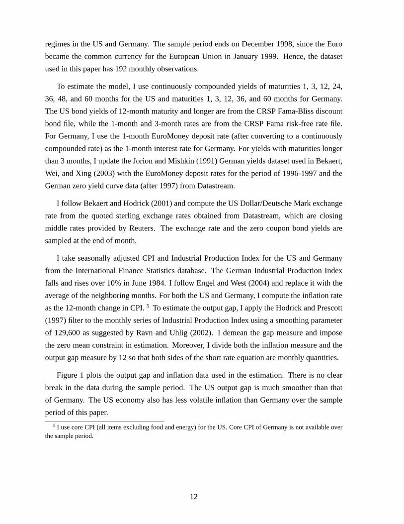
Figure 1 plots the output gap and inflation data used in the estimation. There is no clear

break in the data during the sample period. The US output gap is much smoother than that

of Germany. The US economy also has less volatile inflation than Germany over the sample

period of this paper.

5 I use core CPI (all items excluding food and energy) for the US. Core CPI of Germany is not available overthe sample period.

12

3.2 Identification and Estimation

The structural VAR is not sufficient to exactly identify all the parameters, because latent factors

can be arbitrarily scaled and rotated to produce observationally equivalent systems. To exactly

identify the latent factor processes, I pin the mean of each latent factor to be zero and ensure

that the model matches the mean of the short rate in the data (see Appendix C).

I estimate the model with MCMC. There are three main reasons why I use a Bayesian

estimation method. First, the Bayesian estimation method can handle the nonlinear observation

equation of the depreciation rate without any approximation. Previous papers, such as Han

and Hammond (2003) and Inci and Lu (2004), use the maximum likelihood estimator and an

extended Kalman filter, and they must linearize the observation equation for the depreciation

rate. This approximation essentially violates the no-arbitrage condition used to derive the

depreciation rate process, which could introduce large errors.

Second, the Bayesian estimation method is computationally much more tractable. The

model in this paper is high-dimensional and nonlinear in parameters. The parameters are also

constrained, for example, in equation (22). These complexities make a likelihood function with

latent factors hard to optimize. The Bayesian estimation method also infers the latent factors

from all yields and the depreciation rate by assigning a measurement error to each observation

equation.

Third, the Bayesian estimation method provides a posterior distribution of the parameters

and the time-series paths of latent factorsft andf ∗t . From the posterior distribution, I can

compute the finite sample moments of yields and the best estimates (the posterior mean) of the

model-implied depreciation rate and the foreign exchange risk premium.

The Bayesian estimation method also allows the use of prior distribution to incorporate

additional information into the parameter estimation. I follow the literature of Bayesian

estimation of monetary policy rules (e.g., Justiniano and Preston, 2004; Lubik and Schorfheide,

2005) and impose positivity ofδi1,zi andΦf i. and assume a normal prior distribution forΦf i.

with mean[.02, .04, .95] and a diagonal covariance matrix with[.01, .02, 10] on the diagonal.6

6 Compared to the priors used in Justiniano and Preston (2004) and Lubik and Schorfheide (2005) (90% interval[0.12, 0.87] for the long-run response to output and[1.09, 1.89] for long-run response to inflation), the priors inthis paper are much less informative. AssumingΦfifi is fixed at .95, the prior distribution forΦfizi has a 90%interval [0, 3.69] for the long-run response to output gap and[0, 5.45] for long-run response to inflation. Theprior distribution onΦfifi is also noninformative with a variance of 10. Hence, the only informative priors usedin this paper are the positivity of the short rate’s responses to output gap and inflation and the stationarity of theVAR.

13

As in equation (7), the innovations to the depreciation rate are the same shocks toXt as

implied by the no-arbitrage condition. However, previous studies treat the innovations to the

deprecation rate separately from the innovations to the state variables. For example, papers

using Kalman filter techniques, such as Han and Hammond (2003) and Dewachter and Maes

(2001), simply take the conditional variance of the depreciation rate in their estimation and

assume that the innovations to the depreciation rate are unrelated to the factor dynamics. This

approach overlooks the fact that the same shocks to the state variables drive the depreciation

rate as implied by the no-arbitrage condition.

In this study, I ensure that the shocks to macro variables in equation (7) enter the

depreciation rate. With the state variable process defined in equation (15), I can write equation

(7) as

∆st+1 = µst + σs

t εt+1

= µst + σs

t Σ−1(Xt+1 − µ− ΦXt), (26)

where the vector of unobservable shocksεt+1 is replaced by the implied residuals using the

dynamics of the VAR. To break the stochastic singularity for the depreciation rate equation, I

assume an additive measurement error for∆s,

∆st = ∆st + η∆st , (27)

whereη∆st ∼ IID N (0, σ2

η,∆s).

I also assume that all yields are observed with errors, which avoids the arbitrary choice of

selecting a few yields to be measured without errors as in Chen and Scott (1993). Hence, the

observation equations for bond yields are

y(n)t = y

(n)t + η

(n)t , (28)

y∗(n)t = y

∗(n)t + η

∗(n)t , (29)

wherey(n)t andy

∗(n)t are the model-implied yields from equation (23),η

(n)t ∼ IID N (0, σ2

η,n),

andη∗(n)t ∼ IID N (0, σ∗2η,n).

4 Empirical Results

4.1 Parameter Estimates

In Panel A of Table 1, I report the posterior mean and standard deviation of the factor dynamics

of equation (15). The first (second) row ofΦ shows that the US output gap (inflation) can be

14

forecasted by the lagged US output gap (inflation) and lagged latent factor,ft−1. Lagged US

variables significantly enter the German output gap equation. Consistent with Figure 1, the US

output gap process is much smoother than the German output gap process, which is seen by

theΦgg estimate (0.93), compared to the estimatedΦg∗g∗ (0.85). The German macro variables

also have larger conditional variances.

Panel B reports the estimates of the short rate equation parameters. The US short rate

loads positively on the US output gap and US inflation with coefficients 0.171 and 0.636,

respectively. This suggests that the Fed usually increases the short rate when the economy

is operating over its potential and is facing an potentially high inflation. In particular, a 1%

inflation leads to a 63.6 basis points (bp) contemporaneous increase in the US short rate.

The German short rate also loads positively on the German output gap and German

inflation. Consistent with Clarida, Galı, and Gertler (1998), the US short rate significantly

enters the German short rate equation. The coefficient onft is 0.177,7 which suggests that the

Bundesbank increases the German short rate by 17.7 bp per 1% increase of the US short rate

by the Fed.8

To check whether the model in this paper can capture the response to inflation as implied by

the data in a simple OLS regression, I compute the model-implied coefficients of the following

standard Taylor rule

rit = βi

0 + βi1g

it + βi

2πit + νi

t . (30)

The model-implied coefficient is 0.511 (1.157) for the output gap (inflation) for the US. The

corresponding OLS regression coefficient is 0.309 (1.068). For Germany, the model-implied

coefficient is 0.240 (1.150) for the output gap (inflation), which is also very close to the

corresponding OLS regression coefficient 0.148 (1.021). Therefore, the model in this paper

can capture the response to inflation implied by the data in an OLS regression of standard

Taylor rules.

I report the estimates of the market prices of risk in Panel C of Table 1. The estimates ofλ0

andλ∗0 are very close to each other. Moreover, the elements ofλ1 andλ∗1 are also estimated to

7 As in Section 2.3, we can write the German short rate equation asr∗t = δ∗0 + δ∗>1,Z∗Z∗t + δ∗1,rrt + f∗t =

δ∗0 + δ∗>1,ZZt + δ∗>1,Z∗Z∗t + δ∗1,fft + f∗t , whereδ∗1,f = δ∗1,r andδ∗>1,Z = δ>1,Zδ∗1,r. Panel B of Table 1 reports the

estimated parameters with the constraints imposed. Therefore, the coefficient onft is the same as the coefficienton rt.

8 The long-run response to US inflation, as in equation (11), isφfπ

1−φff+ δ1,π = 0.954, which is very close to

1. The long run response to German inflation is estimated atφf∗π∗1−φf∗f∗

+ δ∗1,π∗ = 0.441, which is smaller than 1.However, German inflation is positively correlated with US inflation and this ignores the inclusion of the US shortrate, with its implied policy loading on US inflation, in the German short rate equation.

15

be very close to each other. This is expected from Brandt, Cochrane, and Santa-Clara (2005),

who show that the volatility of the exchange rate and the volatility of the SDFs based on asset

markets imply that the SDFs must be highly correlated across countries. Therefore, the market

prices of risk on the common source of risk assigned by investors in different countries must

be very close to each other. In Brandt, Cochrane, and Santa-Clara (2005), the domestic and

foreign SDFs load equally on priced shocks, and their estimates of the correlation coefficients

between the US SDF and the SDFs of the UK, Germany, and Japan are all above 0.98 with

standard errors of 0.01 or smaller. The correlation between the SDFs of the US and Germany

estimated from my model is 0.99 with a standard error smaller than 0.01. Backus, Foresi, and

Telmer (2001) also report very close estimates of the market prices of risk on the common

factor in their 3-factor interdependence affine term structure model. Market incompleteness or

missing priced risk does not significantly reduce the high correlation between SDFs, as Brandt,

Cochrane, and Santa-Clara (2005) show.

In Panel D of Table 1, I report the estimates of the standard deviations (per month) of the

measurement errors. The standard deviations of the measurement errors are fairly small for all

yields. For the US, the estimates range from 7.01 bp for the one-month yield to 4.50 bp for the

60-month yield. The German yield curve is fitted even better, with the standard deviations of

the measurement errors all around 4 bp. The standard deviation of the measurement error of

∆s has a posterior mean of 3.07% and standard deviation of 0.19%. These estimates suggest

that the model provides a very good fit to the yield curves and a reasonable fit to exchange rate

dynamics.

In Figure 2, I plot the estimated time series of the latent factors and contrast them with

the demeaned short rates. Simple eyeballing suggests that the estimated latent factors do not

resemble the exchange rate level or changes, but in common with many term structure models

with latent and macro factors, the latent factors closely follow interest rate levels. This suggests

that it is not with the latent factors that the model captures the exchange rate dynamics, but with

macro risks.

Matching Moments of Macro Variables and Yields

Table 2 reports the first and second unconditional moments of macro variables and yields

in the data and implied by the model. I compute the standard errors of the data moments using

the General Method of Moments (GMM) with 4 lags. For the moments implied by the model, I

report their posterior standard deviation. Panel A shows that the model provides a close match

to the means, standard deviations, and autocorrelations of the output gap and inflation for both

16

the US and Germany. Note that the output gaps data are demeaned and I impose the zero mean

constraint in the estimation. In summary, Panel A suggests that the factor dynamics in equation

(15) produce a good fit to the dynamics of macro variables in the data.

Panels B and C of Table 2 show that the model of this paper provides a close match to

the means, standard deviations, and autocorrelations of the US and German yields. Because

of the additive IID measurement errors in equations (28) and (29), the standard deviations of

model-implied yields are always slightly lower than their data counterparts by construction.

The extremely high term spread found in the complete affine models of Backus, Foresi, and

Telmer (2001) does not show up in the more flexible essential affine model of this paper.

4.2 Model-Implied Exchange Rate Dynamics

The model-implied depreciation rate∆s in this paper represents the maximum explanatory

power of the included macro variables. In Panel D of Table 2, I present moments of the model-

implied depreciation rate∆s and contrast them with the data. The mean of∆s matches the

mean of the data depreciation rate∆s. The standard deviation of∆s is about 2.3 times smaller

than the data. This is the result of the additive measurement error. The lower volatility of

the model-implied depreciation rate implies that there are factors affecting exchange rates

not included in the model. Some of these may be variables like the current account (see

Hooper and Morton, 1978), or market incompleteness (see Brandt and Santa-Clara, 2002).

The autocorrelation of∆s is 0.206, higher than the 0.021 autocorrelation in the data. This

is becauseµst is very persistent (with an autocorrelation of 0.911), while the model-implied

exchange rate changes are not as volatile as the data. The standard deviation ofµst is estimated

at 0.374, about one-ninth of the standard deviation of the data exchange rate changes∆s,

and one-fourth of the standard deviation of the model implied∆s. Thus, most model-implied

exchange rate movements are unexpected.

In the top panel of Figure 3, I plot the posterior mean of the model-implied depreciation

rate∆s, which is a function of macro variables, together with the data depreciation rate.9 The

correlation between∆s and∆s is 0.616, and theR2 of regressing∆s onto∆s (with a constant)

is 38%. Therefore, a significant proportion of exchange rate movements is explained by macro

9 The model-implied exchange rate change,∆s, successfully reproduces several large movements of the USDollar/Deutsche Mark exchange rate. One interesting episode is the 8.75% depreciation of the Deutsche Mark inOctober 1992, which is associated with the turmoil of the British Pound’s withdrawal from the European MonetarySystem. The model-implied exchange rate change in October 1992 is -4.69%. After decomposing the∆s intothe contributions of each shock toXt in this month, the US (German) monetary policy shock accounts for 21.8%(44.3%) of the 4.69% depreciation. In addition, the German inflation shock accounts for 38.4%.

17

fundamentals. In comparison, empirical studies based on monetary models or NOEM models

find that macro variables can only explain about 10% of the variation of exchange rate changes

in the data. For example, Engel and West (2004) estimate a monetary model using monthly

US/German data and report a correlation of 10% between the model-implied exchange rate

changes and the data. Lubik and Schorfheide (2005) look at US/Euro exchange rate and find

that their estimated model explains 10% of the variation of the exchange rate changes in the

data. The model in this paper improves the fit to the exchange rate by deriving the depreciate

rate process under no arbitrage. Unlike Engel and West (2004) and Lubik and Schorfheide

(2005), UIRP does not hold and thus the exchange rate exposure to macro innovations is

amplified and varies over time due to the time-varying market prices of risk. I explore the

importance of time-varying risk premia with a simulation study below.

The model in this paper links exchange rate changes, instead of the exchange rate level,

to macro fundamentals. However, I can compute the model-implied exchange rate levels from

∆s. In the bottom panel of Figure 3, I plot the level of the exchange rate in the data and that

implied by the model. I define the model-implied exchange rate level as the cumulative sum of

the posterior mean of the exchange rate changes,St = S1 + exp(∑t

i=2 ∆si), whereS1 is the

data exchange rate level at the beginning of the sample period. As we can see in Figure 3, the

model-implied exchange rate level,S, shares the same trend as the exchange rate level in the

dataS and largely tracks the movement ofS. The correlation betweenS andS is 0.874.

Panel D of Table 2 also reports the first and second moments of the exchange rate level in

the data and implied by the model.S matches the autocorrelation of the data exchange rate

level, but has a slightly lower mean. The volatility ofS is about half that of the data, as∆s

has a smaller standard deviation than the depreciation rate in the data. Although not directly

comparable to this paper due to different modeling assumptions, Engel and West (2004) find

that the exchange rate level implied by their model has a variance of about 1/16 of that observed

in the data, while Mark (2005) finds that the model-implied exchange rate level is much more

volatile than the data.

4.3 How Important are Time-Varying Market Prices of Risk?

In monetary models and NOEM models, the exchange rate is a linear function of macro

variables, which we can rewrite in first differences as

∆st = β0 + β1∆rt + β∗1∆r∗t + β2∆gt + β∗2∆g∗t + β3∆πt + β∗3∆π∗t + νt, (31)

18

whereνt is an IID residual. In these models, domestic and foreign macro variables typically

enter the exchange rate equation in differences (see, e.g., Meese and Rogoff, 1983; Engel and

West, 2004). Hence, the coefficients in equation (31) are typically constrained, i.e.,βi = −β∗ifor i = 1, 2, 3.

When estimating the regression (31) on the data used in this paper, I find anR2 of 10.1%

for the unconstrained regression and anR2 of 8.2% for the constrained regression, respectively.

We can view theR2 of unconstrained regression as the upper bound for theR2 that any

model dictating a static linear relationship between the exchange rate and macro variables

can produce. Thus, although macro factors account for 38% of the variation of exchange

rate changes in the model, we cannot capture this link between macro factors and exchange

rates using a standard macro regression like equation (31). I conduct simulation exercises to

illustrate how important this time-varying mapping is and why the static linear regressions as

in (31) typically find little evidence of macroeconomic determination of exchange rates.

I simulate two datasets using the posterior mean of parameters listed in Table 1. First,

I simulate a very long sample (10,000 monthly observations) to compute the population

regression coefficients. Second, I simulate 1,000 samples each with 192 monthly observations.

By construction, the simulated depreciation rate is completely determined by macro variables

since it is generated using equation (7) without measurement error. I find that the mean,

standard deviation, and autocorrelation of the simulated data closely match those of the real

data. The only exception is that the model-generated∆s has lower volatility than observed in

the data, as the model-implied depreciation rate∆s accounts for about 38% of variation of the

data depreciation rate. This is expected from the match of the model-implied exchange rate to

the data in Table 2.

In Table 3, I report the coefficient estimates and theR2 of the regression based on (31)

using the simulated samples. In Panel A, I report the results for unconstrained regressions.

The populationR2 is only 45.2%, even though the depreciation rate is generated under the null

that the depreciation rate is completely determined by macro variables. This suggests that even

with a large amount of observations, the linear regression cannot capture the time-varying link

between macro shocks and the exchange rate.

The small sample regression results suggest that the coefficient estimates have large

standard deviations. The meanR2 is 44.4% with a standard deviation of 12.7%. When the

regression is constrained, the coefficients on the output gap differential and the interest rate

differential are statistically significant. If the US output gap (short rate) increases faster than

the German output gap (short rate) and∆g−∆g∗ (∆i−∆i∗) is above its mean, the dollar tends

19

to appreciate relative to its mean. In the constrained regression, theR2 decreases to 38.0% for

the population regression and the meanR2 of small sample regressions is 29.2%. Taking into

account the fact that the model explains about 38% of the depreciation rate variation in the data,

theR2s of the simulation studies roughly translate into 16.9% (= 0.38× 0.444) and 11.1% (=

0.38× 0.292) for the unconstrained and constrained regressions, respectively. This is a similar

order of magnitude to theR2 of 10.1% (8.2%) for the unconstrained (constrained) regression

when applying equation (31) to the data.

To further illustrate the importance of the time-varying market prices of risk, I simulate

another dataset withλi1 set equal to zero. In this case, the market prices of risk are constant and

the depreciation rate is linked to macro variables in a static and linear fashion. In Panel C of

Table 3, I report the regression results using the second set of simulated samples with no time-

varying risk premia. The standard deviation of the coefficient estimates in small samples are

much smaller and closer to the long sample estimates than the case whenλi1 is not constrained

to be zero as in Panels A and B. TheR2 has a mean of 94.1% and a standard deviation of 0.02,

but is biased upward in small sample compared to the 87.5%R2 for the population regression.

Overall, this suggests that the relation between exchange rate changes and macro variables

can be well captured by the regression based on equation (31), but only in the absence of time-

varying risk premia. However, the signs of coefficients in Panel C do not make much economic

sense, which suggests that the model cannot pick up the true relation between macro variables

and exchange rate movements without the time-varying market prices of risk.

In conclusion, time-varying market prices of risk are important in the mapping of macro

shocks to unexpected exchange rate movements. The static linear relationship dictated by

the monetary models and NOEM models overlooks this important feature. Consequently,

empirical studies based on these linear models tend to find little evidence that exchange rates

are related to macro fundamentals, even though there may be a tight link between macro

variables and exchange rates.

4.4 The Foreign Exchange Risk Premium

In this section, I study the time series property of the model-implied foreign exchange risk

premium. Fama (1984) shows that the deviations from UIRP translate into two necessary

conditions on the moments of the foreign exchange risk premium. First, the foreign exchange

risk premiumrpt is negatively correlated with the interest rate differentialrt − r∗t . Second, the

20

foreign exchange risk premiumrpt has a larger variance thanrt − r∗t :

Corr(rpt, rt − r∗t ) < 0, (32)

|Cov(rpt, rt − r∗t )| > V ar(rt − r∗t ). (33)

In Panel A of Figure 4, I plot the model-implied conditional mean of the exchange rate

changeµs and its components – the interest rate differentialr − r∗ and the foreign exchange

risk premiumrp. The Deutsche Mark is expected to appreciate most of the time in the sample

period, asµs tends to be greater than zero. This is in line with the ex post pattern of the US

Dollar/Deutsch Mark in Figure 3. The foreign exchange risk premiumrp moves closely with

µs, while the interest rate differential is much smoother than bothrp andµs. The standard

deviation ofrp is 1.44% per year, larger than 1.35% per year forµs. Moreover, the foreign

exchange risk premiumrp is negatively correlated with the interest rate differentialr− r∗ with

a correlation coefficient equal to−0.40. These statistics satisfy the Fama (1984) conditions in

equations (32) and (33).

The negative correlation betweenr − r∗ and rp suggests that on average, the currency

carry trade (borrow in currencies with low interest rates and invest in currencies with high

interest rates) is profitable, especially in the early 1990’s during which the US interest rates

are falling and are low relative to German interest rates. Panel B of Figure 4 suggests that the

expected carry trade profit is related to the countercyclical property of the foreign exchange

risk premium. The foreign exchange risk premium has peaks and troughs, and it moves closely

with the output gap differential,g∗ − g. The correlation betweenrp andg∗ − g is 67.8%.

Therefore, when the US economy is sluggish relative to Germany, i.e., wheng∗− g is positive,

the dollar is expected to depreciate and the carry trade of borrowing in the dollar and investing

in the Deutsche Mark commands a higher expected return. Hence, the foreign exchange risk

premium is countercyclical.

In Panel C of Figure 4, I plot the foreign exchange risk premium,rp, together with the

inflation differential between Germany and the US,π∗−π. The inflation differential is negative

most of the time during the sample period. The foreign exchange risk premiumrp tends to

move together withπ∗ − π. The correlation between them is 54.4%, which is lower than the

correlation betweenrp and the output gap differential. Nevertheless, this suggests that a large

proportion of the variation ofrp is due to shocks to the output gap and inflation.

21

4.5 Deviations From the Unbiasedness Hypothesis

According to the UH, the forward premium (equal to the interest rate differential with covered

interest rate parity arbitrage) is an unbiased predictor of future exchange rate changes. It is

often empirically tested by a regression of the following form:

1

n(st+n − st) = αn + βn(yn

t − y∗nt ) + vt,t+n. (34)

If the UH (or UIRP) holds,βn should be equal to one.

Empirical studies find thatβn is negative (see Hodrick, 1987; Engel, 1996), which means

when the interest rate differential is greater than its sample average, currency depreciation is

greater than its sample average (i.e.,∆s is below its sample average).10 This departure from

UIRP is known as forward premium anomaly, as many asset pricing models fail to meet the

Fama (1984) conditions in equations (32) and (33) for a negativeβn coefficient.

Recent studies find that latent factor term structure models can generate negativeβn (see,

e.g., Bansal, 1997; Dewachter and Maes, 2001; Han and Hammond, 2003; Ahn, 2004).

However, these studies use only latent factors and cannot attribute the deviations from UIRP

to macro fundamentals. In comparison, VAR studies (e.g., Eichenbaum and Evans, 1995)

find monetary policy shocks induce a departure from UIRP, but their finding only implies

a deviation from UIRP conditional on a monetary policy shock. Since their VARs do not

explicitly specify and identify the risk premium, they cannot quantify how important monetary

policy shocks are for the unconditional deviation from UIRP studied in the literature, which is

the deviation ofβ1 coefficient from 1. In this section, I quantify the relative contributions of

macro shocks to the deviations from UIRP.

I compute the model-impliedβn coefficient by running the UH regressions in equation (34)

using interest rates and exchange rate changes fitted using the time series of latent factors and

parameters drawn in each iteration of the MCMC estimation. I compute the fitted exchange

rate changes over horizons beyond one month as the sum of fitted one month changes.

In Panel A of Table 4, I report the UH test results. The point estimate of UH test coefficient

estimated with the data is negative at the one-month horizon, then gradually turns positive. This

is consistent with the finding in Chinn and Meredith (2005). The model-implied coefficients

show similar pattern. For example, the one-month horizon coefficient is -0.014 for the model

and -0.262 for the data.11 For the 12-month horizon, the model implied coefficient is 0.218,

10 It is worth noting that Boudoukh, Richardson, and Whitelaw (2006) recast the UIRP condition in terms offuture exchange rate changes against forward interest rate differentials and find much more support for the theory.

11 The β1 based on the simple regression in equation (34) is not statistically significant from one. However,

22

compared to 0.517 estimated with the data.

I can quantify the relative contributions of macro shocks to the deviation from UIRP by

decomposing and attributing the total deviation to the risk premium associated with each macro

shock. SinceEt(∆st+1) = rt− r∗t + rpt, I can express the slope coefficientβ1 in equation (34)

as

β1 =Cov(rt − r∗t + rpt, rt − r∗t )

V ar(rt − r∗t )= 1 +

Cov(rpt, rt − r∗t )V ar(rt − r∗t )

. (35)

It is easy to see that the slope coefficientβ1 can be negative as found in the data only if the

Fama (1984) conditions in equations (32) and (33) are satisfied.

Note that the total foreign exchange risk premium is the sum of the risk premium assigned

to each macro shock, i.e.,rpt =∑

j rpjt , whererpj

t = (λ>t,j − λ∗>t,j )λt,j andλit,j is the element

on thej-th row of λit for j = g, π, g∗, π∗, f, f ∗. Since the covariance operator is linear, we

have

β1 = 1 +Cov(rpt, rt − r∗t )

V ar(rt − r∗t )= 1 +

∑j Cov(rpj

t , rt − r∗t )

V ar(rt − r∗t ). (36)

In Panel B of Table 4, I present the decomposition results.12 The risk premium associated

with the US output gap shocks contributes little to the deviation ofβ1 from 1, while the German

output gap risk premium makes the deviation less severe by contributing a positive number to

β1. The US (German) inflation risk premium contributes about 12% (13%) of the deviation

from UIRP. Risk premia associated with monetary policy shocks are most important in driving

β1 from 1. The risk premium associated with US monetary policy shocks leads to a deviation

of −0.187 ofβ1 from 1, about 18% of the total deviation. The risk premium associated with

German monetary policy shocks have the lion’s share onβ1 by contributing−0.831 to the

total deviation of−1.055. Eichenbaum and Evans (1995) find that US monetary policy shocks

induce a departure from UIRP. The results in this paper reveal that in terms of contribution

to the deviations from UIRP, German monetary policy shocks are more important than US

monetary policy shocks, and that inflation shocks also play an important role.

this does not mean that UIRP holds. A Bayes factor test strongly rejects the hypothesis of constant risk premium,under which UIRP holds, in favor of time-varying risk premium. Failing to reject the UH in a univariate regressionmay due to the low power of the test. Chinn and Meredith (2005) and Bekaert, Wei, and Xing (2003) use eitherlonger sample or VAR-based tests and reject the short horizon UH using US/German data. Recently, Dittmarand Thornton (2004) shows that adding macro information increases the power of EH tests. In Section 4.4, theoutput gap differential and inflation differential clearly contain information of the foreign exchange risk premium.Therefore, I addg∗ − g andπ∗ − π to the right hand of the UH regression. I find that the short horizon UH isrejected at the 10% level in the expanded regression test with Hodrick (1992) standard errors.

12 I compute the decomposition of the deviation ofβ1 from 1 computed using the estimated model. The Jensen’sterm as in equation (8) has minimal effect (less than 1%) on the deviation ofβ1 from 1, thus I do not include it inthe decomposition.

23

4.6 What Drives Exchange Rate Dynamics?

I now investigate the source of variation in exchange rate changes. Specifically, I compute

variance decompositions ofµst , rpt, ∆st, andfpn

t from the model. I ignore measurement

error in the depreciation rate when computing the variance decompositions. Asµst , rpt, and

∆st are nonlinear functions ofXt, I compute the variance decompositions using Monte Carlo

simulations conditional on each observation in my sample as in Iwata and Wu (2005). I

simulate the model by drawing random shocksεt+i (i = 1, . . . , 120) fromN (0, I). Conditional

on an observation ofXt, I compute the evolution ofX using equation (15). I use equations

(7) and (8) and compute the forecast errors,Vt+n − Et(Vt+n) for V = µs, rp, and∆s, due

to each component ofε for n = 1, 3, 12, 60, 120. This process is repeated1, 000 times. The

variance decompositions are computed as the percentage of the sample variance of the forecast

error due to each element ofε of the variance of the total forecast errors. The simulation-based

variance decomposition method produces the same results for linear systems as standard VAR

technique.13

Panel A of Table 5 reports the variance decompositions ofµs for various forecast horizons.

At short horizons, shocks to output gaps and inflations are responsible for more than 75% of

the variation inµs. The latent factorsft andf ∗t , whose shocks are monetary policy shocks,

explains more variation inµs as the horizon increases, ranging from 24.1% for the 1-month

horizon to about 34.9% for the 120-month horizon. The last column of Panel A reports the

total mean squared forecast errors (MSE), which increases as the forecast horizon increases

and converges to the unconditional variance ofµs.

In Panel B of Table 5, I report the variance decompositions of the foreign exchange risk

premiumrpt, whose variance indicates deviations from UIRP, for various forecast horizons.

Together, the output gap and inflation account for about 80% (70%) of the variation of the

foreign exchange risk premium over the 1 (120) month forecast horizon. This is consistent

with Panels B and C of Figure 4. Note that this result is not in conflict with the finding in

Section 4.5 that risk premia associated with monetary policy shocks are responsible for most

of the deviation ofβ1 from 1 at the one-month horizon, as it is the covariance betweenrpt and

rt − r∗t that determines the deviation ofβ1 from 1. The MSE increases over forecast horizons

and converges to the unconditional variance ofrp. Moreover, the MSE of forecastingrpt is

larger than that ofmust for all horizons and the unconditional variance ofrpt is also larger than

13 An alternative approach is linearizingµst+n, rpt+n, and∆st+n by Taylor expansion and applying the VAR

techniques for variance decompositions. I find that it delivers variance decomposition results similar to thesimulation approach used in this paper.

24

µst , which implies thatrpt is negatively correlated withrt − r∗t . This is consistent with the

negative slope coefficient in the UH test regression and the statistics reported in Section 4.4.

I report the variance decompositions of∆s for various forecast horizons in Panel C of Table

5. The MSEs over various horizons are close to each other and also close to the unconditional

variance of∆s, because most of the variation of∆s is due to unexpected movements. The

output gap and inflation each accounts for about 10-17% variation of∆s. Monetary policy

shocks (innovations toft and f ∗t ) are responsible for about 60% (50%) of the variance of

forecasting∆s for short (long) horizons. US monetary policy shocks alone account for about

40% of the variance of forecast errors. This finding is consistent with previous studies. For

example, Clarida and Galı (1994) find that above 40% of the variance of forecasting the change

in the real US Dollar/Deutsche Mark exchange rate for various horizons (ranging from 1 to 20

quarters) is due to monetary shocks. Eichenbaum and Evans (1995) also find that shocks to US

monetary policy contribute 43% to the variability of the US Dollar/Deutsche Mark exchange

rate in their benchmark specification. However, VARs studies cannot gauge how important

the risk premium is in driving the variation of exchange rates, while the departure from UIRP

implies volatile risk premia. Panel B and Panel C suggest thatrp unconditionally accounts

for about 10% of the total variation of∆s. However, over short forecast horizons, the foreign

exchange risk premium is less important. For example, over a 1-month horizon,rp accounts

for only 1.3% of the total variation of exchange rate changes.

In Panel D of Table 5, I report the unconditional variance decomposition of the forward

premium,fpnt = fn

t − st = ynt − y∗nt . I compute the unconditional forecast variance using a

horizon of 240 months. Monetary policy shocks account for more than 55% of the variation of

the forward premium across all maturities. The German output gap is also important in driving

variations in the forward premium, accounting for 40% (30%) of the variation of the forward

premium in the short (long) run. The US output gap and inflation account for little variation

in the forward premium, as they enter both the US interest rates and German interest rates and

their effects tend to cancel out.

The last column of Panel D of Table 5 reports the proportion of the unconditional variance

decompositions of the forward premium due to risk premia. Sincefpnt = yn

t − y∗nt = an +

bnXt−(a∗n +b∗nXt), I follow Ang, Dong, and Piazzesi (2004) and partition the bond coefficient

bin onXt into an EH term and into a risk-premia term:

bin = bi,EH

n + bi,RPn ,

where I compute thebEHn bond pricing coefficient by setting the market prices of riskλi

1 = 0. I

let ΩF,h stand for the forecast variance of the factorsXt at horizonh, whereΩF,h = var(Xt+h−

25

Et(Xt+h)). Since yields are given byyi,nt = ai

n +bi>n Xt, the forecast variance of then-maturity

forward premium at horizonh is given by(bn−b∗n)>ΩF,h(bn−b∗n). I compute the unconditional

forecast variance using a horizon of 240 months.

I decompose the forecast variance of yields as follows:

Risk Premia Proportion=(bRP

n − b∗,RPn )>ΩF,h(bRP

n − b∗,RPn )

(bn − b∗n)>ΩF,h(bn − b∗n).

This risk premia proportion reports only the pure risk premia term and ignores any covariances

of the risk premia with the state variables.

The column under the heading “Proportion Risk Premia” in Panel E of Table 5 reports the

proportion of the forecast variance attributable to time-varying risk premia. The remainder

is the proportion of the variance implied by the predictability embedded in the VAR dynamics

without risk premia, under the EH. As the maturity increases, the importance of the risk premia

increases. Risk premia play important roles in explaining the forward premium over longer

maturities. Unconditionally, the pure risk premia proportion of the 60-month forward premium

is 28.7%.

4.7 Impulse Responses of Exchange rates

In this section, I compute impulse response functions to gauge the effect of various macro

shocks on the exchange rate. As∆st and rpt are nonlinear functions ofXt, I follow the

literature on nonlinear impulse responses (Gallant, Rossi, and Tauchen, 1993; Koop, Pesaran,

and Potter, 1996; Potter, 2000) and treat the nonlinear impulse response function as the

difference between a pair of conditional expectations while averaging out the future shocks.

For example, the response ofst+h to a current shockνt is

E(st+h|Ωt−1, νt)− E(st+h|Ωt−1), (37)

whereΩt−1 stands for the set of information available att− 1.

I follow Koop, Pesaran, and Potter (1996) and generate random shocksεt+h fromN (0, I)

to compute sample paths ofst+h for h = 1, 2, 3, . . . 60, from the given initial conditionsΩt−1

andνt. For example, for responses to 1% shock tog, νt is the scaled column corresponding

to g in Σ in equation (15) so that the shock tog is 1% (annualized). Each sample path is

repeated ten times and the two averages of the 10 paths (with and withoutνt) are recorded as

one outcome. This process is repeated 500 times and the conditional expectation in equation

(37) is estimated as the average of the outcomes. I compute the impulse response functions

26

conditional on each observation ofXt. I plot the mean and one-standard-deviation bands for

the impulse response functions.

Impulse Responses of the Exchange Rate Level

Figure 5 plots the responses of the exchange rate to 1% shocks to the output gap, inflation,

and monetary policy. On average, a 1% shock to the US (German) output gap leads to an

immediate 0.6% (0.3%) appreciation for the dollar (Mark). After the shock, the dollar (Mark)

keeps appreciating up to 2.2% (1%) after 20 months. Therefore, economic growth strengthens

the currency. On average, the Mark depreciates by 0.8% immediately after a 1% shock to

German inflation and keep depreciating up to 3.2% after 20 months. In contrast, a 1% shock to

US inflation appreciates the dollar, which is not consistent with the Dornbusch (1976) model,

as the long run PPP condition in the Dornbusch (1976) model will lead to a depreciation of

the dollar in both the short run and the long run. One explanation is related to the monetary

policy rule. An increase of US inflation leads to a 67 bp contemporaneous increase of the US

short rate, as the Fed sets the short rate following the reaction function in equation (11) in the

model. The Fed increases the US short rate in the future from an initial shock to US inflation

today due to the policy inertia in equation (11), which may lead to long run appreciation of

the dollar. Therefore, bad news about inflation may be good news for the exchange rate. This

phenomenon arises in the model of Clarida (2004), who shows that if central banks follow

Taylor rules, a shock that pushes up inflation may trigger an aggressive rise in nominal interest

rates that causes the nominal exchange rate to appreciate in the short run and long run.

I overlay the impulse response function withλit set to be its sample mean in thin solid lines

in Figure 5.14 Constant market prices of risk lead to very different impulse responses after

the initial shock, which are often in opposite directions compared to responses under time-

varying risk premia. This discrepancy is because under constant risk premia, the exposure of

the exchange rate to the macro shocks is no longer state-dependent, and the conditional mean of

∆s is simply the interest rate differential (plus constant risk premia). Again, this suggests that

the time-varying market prices of risk are important in driving the dynamics of the exchange

rate.

In the last column of Figure 5, a contractionary US (German) monetary policy shock

appreciates the dollar (Mark). Both exhibit overshooting as in the model of Dornbusch (1976).

The US dollar achieves its maximal response contemporaneously. In comparison, the Mark

14 I find similar impulse response functions based on a separate estimation of the model under constant marketprices of risk.

27

exhibits a delayed overshooting, as it achieves its maximal response about 20 months after

the shock. In a VAR study, Eichenbaum and Evans (1995) find a delayed overshooting of US

monetary policy shock but Faust and Rogers (2003) find that the delayed overshooting result is

sensitive to identification assumptions. The last column of Figure 5 suggests that the delayed

overshooting result is also sensitive to the nature of the risk premia. With constant risk premia,

there is no delay in the responses the dollar/Mark exchange rate to monetary policy shocks.

The last row of Figure 5 plots the responses of the exchange rate to 1% shocks to the US

short rate, German short rate, and the interest rate differential. I construct a 1% interest rate

shock by shocking all of the state variables in proportion to their Cholesky decomposition

so that the sum of the shocks leads to a 1% (annualized) interest rate shock. These impulse

responses all have wide one-standard-deviation bands, which is in line with the large standard

errors and smallR2 in the UH regression tests. On average, a 1% shock to the US short rate

leads to a 2.2% appreciation of the dollar and the dollar keeps appreciating up to about 3.3%

after 60 months. A 1% shock to the German short rate leads to a 1.8% depreciation of the

Deutsche Mark, which may reflect the influence of the increase of the US short rate after the

shock. To get a better measure, I construct a 1% shock to the interest rate differentialrt−r∗t . In

the last plot, a 1% shock tort − r∗t makes the dollar appreciate about 7% and the appreciation

lasts for a long time, which is consistent with the persistent deviations from UIRP observed in

the data.

Impulse Responses of the Deviations from UIRP

Under UIRP, the impulse response functions of foreign exchange risk premium,rpt, as in

equation (8), should be identically equal to zero. Therefore, large responses ofrpt represent

deviations from UIRP, which the model generates through the prices of riskλt andλ∗t . Figure

6 plots the responses of the foreign exchange risk premiumrpt to output gap shocks, inflation

shocks, and monetary policy shocks conditional on each observation ofXt.15 Shocks to the

output gap, inflation, and monetary policy all generate nonzero initial responses ofrp. Therp

responses fade out monotonically, but are persistent and converge to zero only around 20 to 30

months. The output gap shocks and German monetary policy shocks have the most persistent

effect onrp, lasting about 60 months. The impulse response results are consistent with the

finding in Section 4.5 that deviations from UIRP are larger at short horizons and the UH holds

better over longer horizons. Eichenbaum and Evans (1995) and Faust and Rogers (2003) also

find that monetary policy shocks lead to deviations from UIRP in the sense that responses of

15 I include the Jensen’s inequality term in therpt as in equation (8), but excluding the Jensen’s inequality termmakes very little difference to the impulse response functions.

28

the VAR-implied expectation of ex post excess returns are nonzero. Since their VARs do not

price the term structure together with exchange rates, they cannot link term structure responses

to exchange rate movements. However, an interesting question is what happens to the term

premia when the foreign exchange risk premium responds to shocks that push up the short rate

by 1%. I now investigate the responses ofrpt and the term spread to 1% interest rate shocks.

The third row of Figure 6 plots the responses of the foreign exchange risk premium to a 1%

shock to the US short ratert, German short rater∗t , and the interest rate differentialrt − r∗t .

A 1% shock to the US short rate leads to a decrease inrp. In comparison, a 1% shock to the

German short rate makes therp slightly increase, but this increase is not significant from zero.

Both cases imply a negative correlation betweenrt − r∗t andrpt. A 1% shock to the interest

rate differential produces a−0.7% decrease on average inrpt and converges to zero in about

12 months. The wide one-standard-deviation bands suggest a large amount of uncertainty and

a variable foreign exchange risk premium.

The last row of Figure 6 plots the responses of the term spread,spit = yi,60

t − rit, to a 1%

short rate shock. Note that the foreign exchange risk premiumrpt is from the perspective of

a US investor. From the perspective of a German investor, the foreign exchange risk premium

is rp∗t = −rpt. By comparing the last two rows of Figure 6, we can see that the term spreads

move in the same direction as the foreign exchange risk premium in response to a 1% short rate

shock. For example, a 1% shock to the US (German) short ratert (r∗t ) leads to a decrease of the

term spreadspt (sp∗t ) and at the same time decreases therpt (rp∗t ). As the German interest rates

have a exposure to the US short rate in the model, I compute the responses of the German term

spread to a 1% shock to the US short rate. In the last column, we can see that 1% shock to the

US short rate increasessp∗t , while it also increases (decreases)rp∗t (rpt). These results suggest

that interest rate risk premia and the foreign exchange risk premium tend to move together as

they are driven by the same macro fundamentals.

4.8 Deviations From Purchasing Power Parity

In this section, I investigate the model-implied deviations from the relative PPP in expectation.

If relative PPP in expectation holds, we have:

Et(st+n − st) = Et(πt,t+n − π∗t,t+n), (38)

whereπt,t+n stands for inflation over the period fromt to t + n.

Relative PPP in expectation is a weak form PPP among various PPP definitions, as it

29

dictates that expected exchange rate changes are equal to the expected inflation differential.

Froot and Ramadorai (2005), among others, assume that relative PPP in expectation holds in

the long run as a transversality condition. How good is this assumption? What drives deviations

from relative PPP in expectation? To investigate these questions, I define the deviation from

relative PPP in expectation overn months, DPPPn, as:

DPPPn ≡ 1

n[Et(st+n − st)− Et(πt,t+n − π∗t,t+n)], (39)

In Figure 7, I plot the model-implied deviations from relative PPP in expectation over

1, 12, and 120 months. Clearly, for the 1-month horizon, the deviation from relative PPP in

expectation is large and volatile, and resembles the conditional mean of exchange rate changes,

µs. DPPP monotonically becomes less volatile as the horizon gets longer. For the 120-month

horizon, the deviation is much smaller, ranging from -2% to 6% per year. It shows some mean

reversion property in the 1980’s but it does not show a clear tendency to damp to zero in the

late 1990’s. The deviation from relative PPP implied by the model is in line with the finding in

the literature that short-run deviations from PPP are large and volatile, and that exchange rates

tend toward PPP in the long run but the speed of convergence is extremely slow (see, Rogoff,

1996). However, the model implies that the mean of long run deviation,E(DPPP∞), is 3.29%

with a standard deviation of 0.146%.

I investigate the source of variation in deviations from relative PPP over different horizons

by computing variance decompositions. In Panel E of Table 5, I report the unconditional

variance decompositions of DPPPn using a forecast horizon of 120 months. The variance

decompositions for DPPP1 are very close to that ofµs, including the total MSE. This is

consistent with the fact that the deviation from PPP is large at short horizons and DPPP1

resemblesµs, as shown in Figure 7. Consistent with Figure 7, the total MSE drops

monotonically asn increases. Overall, shocks to German output gap and US monetary policy

shocks drive most of the variation in DPPP over all horizons. Shocks to US output gap are

important for the short horizon deviation from PPP, accounting for about 20% of the forecast

variance of DPPP1, but are less important over longer horizons.

5 Conclusion

This paper builds a no-arbitrage model to understand the dynamics of exchange rates with

macro risks and monetary policy. I incorporate macro variables as factors in a term structure

model by assuming that central banks set short term interest rates in response to the output

30

gap and inflation and using a factor representation for the stochastic discount factors. In the

model, exchange rate changes are the ratio of domestic and foreign stochastic discount factors.

Interest rate differentials across countries and risk premia determine expected exchange rate

changes, similar to finance models of exchange rates. Innovations to macro variables drive

the unexpected exchange rate changes as in monetary models of exchange rates, but scaled by

time-varying market prices of risk.

I estimate the model with US/German data. The model implies a countercyclical foreign

exchange risk premium with macro risk premia playing an important role in matching

deviations from UIRP. After decomposing the total deviation to each macro shock, I find that

monetary policy shocks account for about 90% of the deviation from UIRP at short horizons.

I find that more than 70% of the variance of forecasting the foreign exchange risk premium is

due to the output gap and inflation of both countries. About 50% of the variance of forecasting

exchange rate changes is due to monetary policy shocks. I also compute impulse response

functions of the exchange rate to macro shocks. The responses of the exchange rate exhibit

over-shooting to monetary policy shocks and are consistent with the deviations from UIRP.

The time-varying market prices of risk are essential to link the macro shocks to unexpected

exchange rate movements. The static linear relationship dictated by many monetary models

overlooks the relation, and consequently, tends to find little evidence of the relationship

between macro variables and exchange rates. I find that the correlation between model-implied

exchange rate changes and the data is over 60%. I compute variance decompositions from the

model and find that time-varying risk premia unconditionally account for about 10% of the

variation of the exchange rate changes and 28.7% of the variation of the long-term forward

premium.

Interesting extensions of the model considered in this paper are to impose more structure

on the stochastic discount factor and the factor dynamics, for example, allowing the exchange

rate to also affect output and inflation. Other interesting extensions include expanding the state

variable vector to include other factors that may affect the exchange rates.

31

Appendix

A Exchange Rate Factors

In this appendix, I discuss how statistical inference based on the SDFs introduced in Section 2.1 will be affectedif there are factors orthogonal toXt affecting exchange rates. I assume that the SDFs have an exchange ratecomponent,N i

t+1, defined aslog(N it+1) = − 1

2ωi>ωi − ωi>ξt+1, whereξ is related to certain exchange ratefactors. A common modeling assumption is thatξ is orthogonal toε in equation (1) (see, e.g., Brandt and Santa-Clara, 2002; Leippold and Wu, 2004).

Brandt and Santa-Clara (2002) point out that the exchange rate riskξ and its market prices of riskωi arenot well identified. Some economic sources forωi could be the current account, terms of trade or marketincompleteness. Without loss of generality, I assumeξ is a scalar summarizing all risks related to exchangerates but orthogonal toε andωi is a scalar constant. The depreciation rate with the presence of exchange ratefactors is then

∆st+1 ≡ st+1 − st = m∗t+1 −mt+1 + n∗t+1 − nt+1 (A-1)

= rt − r∗t +12(λ>t λt − λ∗>t λ∗t ) + (λ>t − λ∗>t )εt+1 +

12(ω2 − ω∗2) + (ω − ω∗)ξt+1

= ∆st+1 +12(ω2 − ω∗2) + (ω − ω∗)ξt+1

where I denote the model-implied (as in Section 2.2) depreciation rate as∆st+1.

As ωi is constant and only enters the drift of∆s through the Jensen’s inequality term, andξ is orthogonalto ε, they will not affect studying issues that involve only the drift, such as the forward premium anomaly (seeBrandt and Santa-Clara, 2002). Therefore, I can treat the unspecified residual of∆s, (ω − ω∗)ξt+1, as an IIDmeasurement error of∆s.

The measurement error not only captures model misspecification by serving as a proxy for unspecifiedexchange rate factors, but also breaks the stochastic singularity of the depreciation rate equation. Without themeasurement error, the estimation procedure attempts to fit the depreciation rate based on the tightly restrictedequation (6), which may result in implausible estimates. Effectively, I focus on how much variation of∆s in thedata can be explained by the output gap, inflation, and monetary policy shocks, while leaving the unexplainedvariation of∆s to a measurement error.

B Factor Dynamics from a Structural VAR

To specify the the process forZt, I model the US economy as being represented by the following structural VAR:[

Azz0 Azr

0

−γ>1 1

] [Zt

rt

]=

[Az

1µr

]+

[Azz

2 Azr2

(φ− ργ1)> ρ

] [Zt−1

rt−1

]+

[εt

εt,MP

](B-2)

whereµr = (1− ρ)γ0 +µf , andεt ∼ N (0, I) is a structural shock toZt. These structural shocks are assumed tobe uncorrelated, i.e.,E(εtεt,MP ) = 0. The equation in the structural VAR for the short rate is directly from thebackward-looking monetary policy rule in equation (11).

Without additional constraints, the structural VAR in equation (B-2) is not identified. I follow Bernankeand Blinder (1992) and assumeAzr

0 = 0. That is, monetary policy actions affect output and inflation with alag. As this paper uses monthly data, this is a plausible identification assumption. Furthermore,Azz

0 is assumedto be a lower-triangular matrix. This is a common assumption in recursive identification schemes used in manymonetary structural VAR papers, such as Christiano, Eichenbaum and Evans (1996). With the above identificationassumptions, theZt equation in the structural VAR can be written as

Zt = a1 + a>2 Zt−1 + a3rt−1 + Σzεt, (B-3)

wherea1 = (Azz0 )−1Az

1, a>2 = (Azz0 )−1Azz

2 , a3 = (Azz0 )−1Azr

2 , andΣz = (Azz0 )−1. Σz is a lower-triangular

matrix as a result of the lower-triangularAzz0 . Thert equation in (B-2) remains unchanged withεt,MP identified

32

as the monetary policy shock in the backward-looking monetary policy rule. I refer to equation (B-3) as theidentified VAR.

Replacingrt−1 in equation (B-3) withZt−1 andft−1 as in equation (9), I can write the joint dynamics ofZt

andft, the factors driving the US short rate, as[

Zt

ft

]=

[a1 + a3γ0

µf

]+

[a>2 + a3γ

>1 a3

φ> ρ

] [Zt−1

ft−1

]+

[Σz 00 σf

] [εt

εt,MP

]. (B-4)

In Section 2.3, I discuss the advantages of using equations (B-4) and (9) instead of their equivalentrepresentation of equations (10) and (B-2).

I assume that the German economy can be represented by the following structural VAR:[

Bz∗r0 Bz∗z∗

0 Bz∗r∗0

−γ∗2 −γ∗>1 1

] [rt

Z∗tr∗t

]

=[

Bz1

µr∗

]+

[Bz∗r

2 Bz∗z∗2 Bz∗r∗

2

−ρ∗γ∗2 (φ∗ − ρ∗γ∗1)> ρ∗

][rt−1

Z∗t−1r∗t−1

]+

[ε∗t

ε∗t,MP

], (B-5)

whereµr∗ = (1 − ρ∗)γ∗0 + µ∗f , andε∗t ∼ N (0, I) is a structural shock toZ∗t . I assume that the structural shockε∗t is uncorrelated with the monetary policy shocksε∗t,MP , i.e.,E(ε∗t ε

∗t,MP ) = 0. Furthermore, I assume thatε∗t

andε∗t,MP are orthogonal to the US structural shocksεt andεt,MP , i.e.,E(εtε∗t ) = 0 andE(εt,MP ε∗t,MP ) = 0.

I assume the same recursive identification scheme for the German structural VAR as for the US, but I furtherassume that the German economy is affected by the US short term interest rate only with a lag, so thatBz∗r

0 = 0.Hence, the identified VAR for the German macro variableZ∗ takes the form:

Z∗t = b1 + b>2 Z∗t−1 + b3rt−1 + b4r∗t−1 + Σz∗ε

∗t , (B-6)

whereb1 = (Bz∗z∗0 )−1Bz

1 , b>2 = (Bz∗z∗0 )−1Bz∗z∗

2 , b3 = (Bz∗z∗0 )−1Bz∗r

2 , b4 = (Bz∗z∗0 )−1Bz∗r∗

2 , andΣz∗ =(Bz∗z∗

0 )−1. Σz∗ is a lower-triangular matrix as a result of the lower-triangularBz∗z∗0 .

Substitutingrt−1 andr∗t−1 in equation (B-6) with equations (9) and (12), and collecting equations (B-4) and(13), I can write the joint dynamics ofXt = [Zt, Z

∗t , ft, f

∗t ]> as follows:

Xt = µ + ΦXt−1 + Σεt (B-7)

Zt

Z∗tft

f∗t

=

µz

µz∗

µf

µf∗

+

a>2 + a3γ>1 0 a3 0

κγ>1 b>2 + b4γ∗>1 κ b4

φ> 0 ρ 00 φ∗> 0 ρ∗

Zt−1

Z∗t−1ft−1

f∗t−1

+

Σz 0 0 00 Σz∗ 0 00 0 σf 00 0 0 σf∗

εt

ε∗tεt,MP

ε∗t,MP

,

whereµz = a1 + a3γ0, µz∗ = b1 + b4γ∗0 + κγ0, κ = (b3 + b4γ

∗2 ).

The parameters in equation (B-7) are constrained. In particular, one constraint is

Φz∗z = Φz∗fγ>1 , (B-8)

as indicated by boxes in equation (B-7). The constraint is the result of mapping from the SVAR to the reducedVAR by substituting the lagged short rate in equation (B-6) with the short rate equation (9). This constraint isimposed in the estimation.

C Econometric Identification

Dai and Singleton (2000) provides identification conditions for latent factor affine term structure models. For thetwo-country Gaussian model considered in this paper, my identification strategy is to set the mean of the latent

33

factorsFt ≡ [ft f∗t ] to zero and pin downδ1,f andδ∗1,f∗ , while letting the conditional varianceσ2f andσ2

f∗ be

unconstrained. To ensure thatFt is mean zero, I parameterizeµ =[

µz µ∗z µf µ∗f]>

so thatµf andµ∗f satisfy

the equation:e>i (I − Φ)−1µ = 0, i = 5, 6

whereei is a vector of zeros with a one in thei-th position. I setδ1,f = 1 andδ∗1,f∗ = 1 as implied by equations(9) and (12). Similar identification strategies have been applied in Ang, Dong, and Piazzesi (2004), Dai andPhilippon (2004), and Bikbov and Chernov (2005). I also impose zero mean on output gapsg andg∗.

To match the mean of the short rate in the sample, I setδ0 in each Gibbs iteration so that

δ0 = r − δ>1 X, δ∗0 = r∗ − δ∗,>1 X, (C-9)

wherer (r∗) is the average US (German) short rate in the data andX is the time-series average of the factorsXt.This means thatδ0 andδ∗0 are not individually drawn as separate parameters, butδ0 andδ∗0 change their value ineach Gibbs iteration because they are functions ofδ1 andδ∗1 .

D Estimating the Model

I estimate the model by MCMC with a Gibbs sampling algorithm. Lamoureux and Witte (2002), Mikkelsen(2002), Bester (2003), and Johannes and Polson (2005) develop similar Bayesian methods for estimating termstructure models, but their settings do not have macro variables. Ang, Dong, and Piazzesi (2004) develop Bayesianmethods for estimating term structure models with both latent and macro variables, but their observation equationsare all linear.

The parameters of the model areΘ = [ µ, Φ, Σ, δ0, δ1, λ0, λ1, δ∗0 , δ∗1 , λ∗0, λ∗1, ση], whereση denotes the

vector of measurement error volatilities[ σ(n)η , σ

(n)η∗ , σ∆s

η ]. The latent factor vectorF is also generated in eachiteration of the Gibbs sampler. I simulate 50,000 iterations of the Gibbs sampler after an initial burn-in period of10,000 iterations.

I now detail the procedure for drawing each of these variables. I denote the factorsX = [Z,Z∗, F ] =XtT

t=1, the set of yields for all maturities in data asY = ynt T

t=1, andY ∗ = y∗,nt Tt=1, and∆s = ∆stT

t=1.

Drawing the latent factor Ft

The factor dynamics (15), together with the observation equations (27) – (28), imply that the model in this papercan be written as a state-space system. The state equation for the system are Gaussian and linear inFt, but alsoinvolve the macro variablesZt andZ∗t . The observation equations for the yields are linear inFt

y(n)t = an + b>n Xt + η

(n)t , (D-1)

y∗(n)t = a∗n + b∗>n Xt + η

∗(n)t . (D-2)

However, the observation equation for∆s is not a linear function ofFt

∆st+1 = rt − r∗t +12(λ>t λt − λ∗>t λ∗t ) + (λ>t − λ∗>t )Σ−1(Xt+1 − µ− ΦXt) + η∆ss

t . (D-3)

As λt = λ0 + λ1Xt andλ∗t = λ∗0 + λ∗1Xt, ∆st+1 is quadratic inFt and contains cross terms ofFt andFt+1.Classic methods such as MLE and Kalman filter must linearize the∆st+1 equation. The Bayesian estimationmethod can drawFt by single state updating without linearization (see Jacquier, Polson, and Rossi, 1994 and2004).

The joint posterior for the latent factor vectorFt can be written as

P (Ft|F−t, Z, Z∗, Y, Y ∗, ∆s,Θ) ∝Ps|Ft︷ ︸︸ ︷

P (∆st|Xt, Xt−1, Θ)P (∆st+1|Xt+1, Xt,Θ)P (Ft|Xt−1, µ, Φ, Σ)P (Ft+1|Xt, µ, Φ, Σ)P (Yt|Xt, Θ)P (Y ∗

t |Xt, Θ)︸ ︷︷ ︸PF Y |Ft

P (Ft), (D-4)

34

whereF−t stands for the vectorF exceptFt, andP (.|µ, Φ, Θ−, X) is the likelihood function forYt ( Y ∗t and

∆st), which is normally distributed from the assumption of normality for the measurement errors in equations(27)–(29).

As the distribution ofFt, P (Ft|F−t, Y, Y ∗, ∆s, Z, Z∗,Θ), is not standard, I use Metropolis-Hastings tosample from it. I assume a flat normal priorP (Ft) for Ft, which is reasonable given thatFt is conditionally normalas in equation (15). The normal distributionPFY |Ft

combined withP (Ft) is a bivariate normal distribution, whichI use as a proposal density forFt. I denote this proposal density asq(Ft) = P (Ft)PFY |Ft

. I draw a candidateFt from q(Ft) then apply a Metropolis step based on the density ofPs|Ft

. The proposal drawFm+1t for the

(m + 1)-th draw ofFt is accepted with probabilityα, where

α = min

P (Fm+1t | Θ, X, Y, Y ∗, ∆s)

P (Fmt | Θ, X, Y, Y ∗, ∆s)

q(Fmt )

q(Fm+1t )

, 1

= min

Ps|F m+1

tPFY |F m+1

tP (Fm+1

t )

Ps|F mt

PFY |F mt

P (Fmt )

P (Fmt )PFY |F m

t

P (Fm+1t )PFY |F m+1

t

, 1

= min

P (∆st|Fm+1t , Zt, Xt−1, Θ)P (∆st+1|Xt+1, F

m+1t , Zt, Θ)

P (∆st|Fmt , Zt, Xt−1, Θ)P (∆st+1|Xt+1, Fm

t , Zt,Θ), 1

. (D-5)

To drawFt at the beginning and the end of the sample, I integrate out the initial and end values ofFt bydrawing from the VAR in (15), following Jacquier, Polson, and Rossi (2004). Since I specify the mean ofF to bezero for identification, I set each generated draw ofF to have a mean of zero.

Drawing µ and Φ

Updatingµ andΦ requires Metropolis algorithms as the conditional posteriors are not standard distributions. Todrawµ andΦ, I note that the posterior ofµ andΦ conditional onX, Y , Y ∗, ∆s and the other parameters is:

P (µ, Φ | Θ−, X, Y, Y ∗, ∆s) ∝ P (Y | Θ, X)P (Y ∗ | Θ, X)P (∆s | Θ, X)P (X | µ, Φ,Σ)P (µ, Φ), (D-6)

whereΘ− denotes the set of all parameters exceptµ andΦ. This posterior suggests an Independence Metropolisdraw, where I first draw a proposal for the(m + 1)-th value ofµ andΦ (µm+1 andΦm+1, respectively) from theproposal density:

q(µ, Φ) ∝ P (X | µ,Φ,Σ)P (µ, Φ),

where I specify the priorP (µ, Φ) to be normally distributed (forΦf andΦf∗ , the prior distribution is a Normaldistribution with mean[ .02, .04, .95] and covariance matrix with diagonal as[ .01, .02, 10] and truncated frombelow at zero. For other parameters, the prior is N(0,1000), consequently,q(µ, Φ) is a natural conjugate normaldistribution. The proposal draw(µ, Φ)m+1 is then accepted with probabilityα, where

α = min

P ((µ, Φ)m+1 | Θ−, X, Y, Y ∗, ∆s)P ((µ, Φ)m | Θ−, X, Y, Y ∗, ∆s)

q(µm, Φm)q((µ, Φ)m+1)

, 1

(D-7)

= min

P (Y | (µ,Φ)m+1, Θ−, X)P (Y ∗ | (µ, Φ)m+1, Θ−, X)P (∆s | (µ, Φ)m+1, Θ−, X)P (Y | (µ, Φ)m, Θ−, X)P (Y ∗ | (µ, Φ)m, Θ−, X)P (∆s | (µ, Φ)m, Θ−, X)

, 1

.

From equation (D-7),α is just the ratio of the likelihoods of the new draw ofµ and Φ relative to the olddraw. I drawµ andΦ separately for each equation in the VAR system (15). As in Bester (2003), I combinethe Independence Metropolis algorithms with Random Walk Metropolis algorithms, but update each row ofΦtogether in both algorithms.

I impose the restriction thatFt is mean zero for identification. I setµi to satisfye>i (I − Φ)−1µ = 0 fori = 5, 6, to ensure that the factorFt has zero mean. Henceµf and µ∗f are simply a function of the otherparameters in the factor VAR in equation (15).

Drawing ΣΣ>

I draw ΣzΣ>z , Σz∗Σ>z∗ , σ2f , andσ2

f∗ separately asΣΣ> is block diagonal. I focus onΣzΣ>z since drawing theother variance parameters is similar. I note that the posterior ofΣzΣ>z conditional onX, Y , Y ∗, ∆s and the other

35

parameters is:

P (ΣzΣ>z | Θ−, X, Y, Y ∗,∆s)

∝ P (Y | Θ, X)P (Y ∗ | Θ, X)P (∆s | Θ, X)P (X | µ, Φ, Σ)P (ΣzΣ>z ), (D-8)

whereΘ− denotes the set of all parameters exceptΣz. This posterior suggests an Independence Metropolis draw.I drawΣzΣ>z from the proposal densityq(ΣzΣ>z ) = P (X | µ, Φ, Σ)P (ΣzΣ>z ), which is an Inverse Wishart (IW )distribution if I specify the priorP (ΣzΣ>z ) to beIW , so thatq(ΣzΣ>z ) is anIW natural conjugate. The proposaldraw(ΣzΣ>z )m+1 for the(m + 1)th draw is then accepted with probabilityα. The accept/reject probability forthe draws ofλs is similar to equation (D-7).

Drawing δ1 and δ∗1

I draw δ1 using a Random Walk Metropolis step:

δm+11 = δm

1 + ζδ1v (D-9)

wherev ∼ N(0, 1) and ζδ1 = .01 is the scaling factor used to adjust the acceptance rate. The acceptanceprobabilityα for δ1 is given by:

α = min

P (δm+11 | Θ−, X, Y, ∆s)

P (δm1 | Θ−, X, Y, ∆s)

q(δm1 | δm+1

1 )q(δm+1

1 | δm1 )

, 1

= min

P (δm+11 | Θ−, X, Y, ∆s)

P (δm1 | Θ−, X, Y, ∆s)

, 1

, (D-10)

where the posteriorP (δ1|Θ−, X, Y, ∆s) is given by:

P (δ1|Θ−, X, Y, ∆s) ∝ P (Y |δ1, Θ−, X)P (∆s|δ1, Θ−, X)P (δ1).

Thus, in the case of the draw forδ1, α is the posterior ratio of the new and old draws ofδ1. I setδ0 to match thesample mean of the short rate. I impose a prior thatδi

1,zi > 0.

Sinceδ∗1 is constrained as in equation (22), I drawδ∗1,3:5 using a Random Walk Metropolis step similar toδ1,but I impose the constraint thatδ∗1,z = δ1,zδ

∗1,f as in equation (22).

Drawing λ0, λ1, λ∗0 and λ∗1

I draw λs with a Random Walk Metropolis algorithm. I assume a flat prior. I draw each parameter separately inλ0 andλ∗0, and each row inλ1 andλ∗1. The accept/reject probability for the draws ofλs is similar to equation(D-10).

Drawing ση

I draw the observation variance(σ(n)η )2 separately from each yield and for the exchange rate changes. I specify

a conjugate priorIG(0, 0.00002), so that the posterior distribution ofσ2η is a natural conjugate Inverse Gamma

distribution, which can be drawn directly as Gibbs sampling. The prior distribution,IG(0, 0.00002), helps keepthe algorithm from over-fitting a certain yield.

E Robustness Checks

In this appendix, I look at several robustness checks. For a model with latent factors, a valid concern is that the fitof a model is due to the latent factors. However, the latent factors in my model have an economic interpretation asthe effect of lagged macro variables and short rate and a monetary policy shock on the current value of the shortrate. As we can see from Figure 2, it is unlikely that the two latent factorsf andf∗ have been stretched to explainthe dynamics of the exchange rate.

36

I also check whether the results are sensitive to the choice of the output gap measure. It is well-known thatthe output gap is estimated with large uncertainty. Hence, I re-estimate the model using the output gap producedby quadratic detrending, as in Clarida, Galı, and Gertler (1998 and 2000). I find the results remain qualitativelythe same. The correlation between∆s and∆s is 0.619, slightly higher than0.616 when the HP filter is used toestimate the output gap. The model still matches the UH coefficients estimated with the data. Another concernis that the output gap is estimated with the full sample data and has a looking-forward bias. As a way to checkwhether my results are robust to this concern, I use the unemployment rate instead of the pre-estimated outputgap and re-estimate the model. The results remain qualitatively the same, with the correlation between∆s and∆s equal to0.620.

As a final check, I re-estimate the model with constant market prices of risk. With constant market pricesof risk, the mapping of macro shocks onto exchange rate movements is no longer state-dependent but constantover time (see equation 7). The model-implied UH regression coefficients are unit for all horizons, since theforeign exchange risk premium is constant under the constrained model. Furthermore, the correlation between∆s and∆s is 0.407, and only 16.6% of the variation of the exchange rate changes in data can be explained bythe constrained model. The results of the constrained estimation emphasize that the time-varying market pricesof risk are responsible for the matching of the deviations from UIRP in the data and the larger proportion of theexchange rate movements explained by the model in this paper.

37

References[1] Ahn, Dong-Hyun, 2004, “Common Factors and Local Factors: Implications for Term Structures and

Exchange Rates,”Journal of Financial and Quantitative Analysis39, 1, 69-102.

[2] Amin, Kaushik, and Jarrow, Robert A.,1991, “Pricing Foreign Currency Options under Stochastic InterestRates,”Journal of International Money and Finance10, 310-29.

[3] Ang, Andrew, and Monika Piazzesi, 2003, “A No-Arbitrage Vector Autoregression of Term StructureDynamics with Macroeconomic and Latent Variables,”Journal of Monetary Economics50, 4, 745-87.

[4] Ang, Andrew, Sen Dong, and Monika Piazzesi, 2004, “No-Arbitrage Taylor Rules”, Working paper,Columbia University.

[5] Backus, David K., Allan Gregory, and Chris I. Telmer, 1993, “Accounting for Forward Rates in Markets forForeign Currency,”Journal of Finance48, 1, 1887-1908.

[6] Backus, David K., Silverio Foresi, and Chris I. Telmer, 2001, “Affine Term Structure Models and theForward Premium Anomaly,”Journal of Finance56, 1, 279-304.

[7] Bansal, Ravi, A. Ronald Gallant, Robert Hussey, and George Tauchen, 1995, “Nonparametric Estimation ofStructural Models for High Frequency Currency Market Data,”Journal of Econometrics66, 251-287.

[8] Bansal, Ravi, 1997, “An Exploration of the Forward Premium Puzzle in Currency Markets,”Review ofFinancial Studies10, 369-403.

[9] Bekaert, Geert, 1996, “The Time Variation of Risk and Return in Foreign Exchange Markets: A GeneralEquilibrium Perspective,”Review of Financial Studies, 9, 427-70.

[10] Bekaert, Geert, and Robert J. Hodrick, 2001, “Expectation Hypotheses Tests,”Journal of Finance56, 1357-94.

[11] Bekaert, Geert, Min Wei, and Yuhang Xing, 2003, “Uncovered Interest Rate Parity and the Term Structure,”Working paper, Columbia University.

[12] Bekaert, Geert, Seonghoon Cho, and Antonio Moreno, 2004, “New-Keynesian Macroeconomics and theTerm Structure,” Working paper, Columbia University.

[13] Bernanke, Ben S., and Alan S. Blinder, 1992, “The Federal Funds Rates and the Channels of MonetaryTransmission.”American Economic Review82, 4, 901-21.

[14] Bester, Alan C., 2003, “Random Fields and Affine Models of Interest Rates,” Working paper, DukeUniversity.

[15] Bikbov, Ruslan, and Mikhail Chernov, 2005, “No-Arbitrage Macroeconomic Determinants of the YieldCurve,” Working paper, Columbia University.

[16] Boudoukh, Jacob, Matthew Richardson, and Robert F. Whitelaw, 2006, “The Information in Long-MaturityForward Rates: Implications for Exchange Rates and the Forward Premium Anomaly, Working paper, NewYork University.

[17] Brandt, Michael W., and Pedro Santa-Clara, 2002, “Simulated Likelihood Estimation of Diffusions withan Application to Exchange Rate Dynamics in Incomplete Markets,”Journal of Financial Ecnonomics63,161-210.

[18] Brandt, Michael W., John H. Cochrane, and Pedro Santa-Clara, 2005, “International Risk Sharing is BetterThan You Think, or Exchange Rates are Too Smooth,” Forthcoming,Journal of Monetary Economics.

[19] Chen, Ren-Raw, and Louis Scott, 1993, “Maximum Likelihood Estimation for a Multi-factor EquilibriumModel of the Term Structure of Interest Rates,”Journal of Fixed Income, 3, 14-31.

[20] Chinn, Menzie D., and Guy Meredith, 2005, “Testing Uncovered Interest Rate Parity at Short and LongHorizons During the Post-Bretton Woods Era,” NBER Working Paper 11077.

[21] Christiano, Lawrence J., Martin Eichenbaum, and Charles Evans, 1996, “The Effects of Monetary PolicyShocks: Evidence from the Flow of Funds.”Review of Economics and Statistics78, 1, 16-34.

[22] Clarida, Richard, and Jordi Galı, 1994, “Sources of Real Exchange rate Fluctuations: How Important areNominal Shocks?”The Carnegie-Rochester Conference Series on Public Policy41, 1-55.

[23] Clarida, Richard, Jordi Galı, and Mark Gertler, 1998, “Monetary Policy Rules in Practice: SomeInternational Evidence,”European Economic Review42, 1033-67.

38

[24] Clarida, Richard, 2004, “Inflation Targeting and Exchange Rate Dynamics: A Classic Model Reinterpreted”,invited lecture at the Central Bank of Mexico, October 2004.

[25] Dai, Qiang, and Kenneth J. Singleton, 2000, “Specification Analysis of Affine Term Structure Models,”Journal of Finance55, 1943-78.

[26] Dai, Qiang, and Kenneth J. Singleton, 2002, “Expectation Puzzles, Time-Varying Risk Premia, and AffineTerm Structure Models of the Term Structure,”Journal of Financial Economics63, 415-41.

[27] Dai, Qiang, and Thomas Philippon, 2004, “Fiscal Policy and the Term Structure of Interest Rates,” Workingpaper, NYU.

[28] Dewachter, Hans, and Konstantijn Maes, 2001,“An Affine Model for International Bond Markets,” Workingpaper, Catholic University of Leuven.

[29] Dittmar, Robert D., and Daniel L. Thornton, 2004, “New Evidence on the Expectations Hypothesis of theTerm Structure of Bond Yields,” Working paper, Federal Reserve Bank of St. Louis.

[30] Dornbusch, Rudiger, 1976, “Expectations and Exchange Rate Dynamics,”Journal of Political Economy84,1161-76.

[31] Duffee, Gregory R., 2002, “Term Premia and Interest Rate Forecasts in Affine Models,”Journal of Finance57,406-43.

[32] Duffie, Darrell, and Rui Kan, 1996, “A Yield-Factor Model of Interest Rate,”Mathematical Finance6,379-406.

[33] Eichenbaum, Martin, and Charles Evans, 1995, “Some Empirical Evidence on the Effects of Shocks toMonetary Policy on Exchange Rates,”Quarterly Journal of Economics110, 4, 975-1009.

[34] Engel, Charles, 1996, “The Forward Discount Anomaly and the Risk Premium: A Survey of RecentEvidence,”Journal of Empirical Finance3, 123-92.

[35] Engel, Charles, and Kenneth D. West, 2004, “Taylor Rules and the DeutschMark-Dollar Real ExchangeRate,” Forthcoming,Journal of Money, Credit, and Banking.

[36] Fama, Euguene, 1984, “Forward and Spot Exchange Rates,”Journal of Monetary Economics14, 319-38.

[37] Faust, Jon, and John H. Rogers, 2003, “Monetary Policy’s Role in Exchange Rate Behavior,”Journal ofMonetary Economics50, 1403-24.

[38] Frankel, Jeffrey A., 1979, “On the Mark: A Theory of Floating Exchange Rates Based on Real InterestDifferentials,”American Economic Review69, 601-22.

[39] Frankel, Jeffrey A., and Andrew K. Rose, 1995, “Empirical Research on Nominal Exchange Rates,” inGrossman and Rogoff (eds.),Handbook of International EconomicsVol. 3, North Holland.

[40] Froot, Kenneth A., and Tarun Ramadorai, 2005, “Currency Returns, Intrinsic Value, and Institutional-Investor Flows,”Journal of Finance60, 3, 1535-66.

[41] Gallant, A. Ronald, Peter E. Rossi, and George Tauchen, 1993, “Nonlinear Dynamic Structures,”Econometrica61, 4, 871-907.

[42] Graveline, Jeremy J., 2006, “Exchange Rate Volatility and the Forward Premium Anomaly,” Working paper,Stanford University.

[43] Han, Bing, and Peter Hammond, 2003, “Affine Models of the Joint Dynamics of Exchange Rates and InterestRate,” Working paper, University of Calgary.

[44] Hodrick, Robert J., 1987,The Empirical Evidence on the Efficiency of Forward and Futures ForeignExchange Markets(Harwood Academic Publishers, Chur, Switzerland).

[45] Hodrick, Robert J., 1989, “Risk, Uncertainty, and Exchange Rates,”Journal of Monetary Economics23,433-59.

[46] Hodrick, Robert J., 1992, “Dividend Yields and Expected Stock Returns: Alternative Procedures forInference and Measurement,”Review of Financial Studies5,3, 357-86.

[47] Hodrick, Robert J., and Edward C. Prescott, 1997, “Postwar U.S. Business Cycles: An EmpiricalInvestigation,”Journal of Money, Credit and Banking29, 1, 1-16.

[48] Hooper, Peter, and John E. Morton, 1978, “Flunctuations in the Dollar: A Model of Nominal and RealExchange Rate Determination,”Journal of International Money and Finance1, 39-56.

39

[49] Hordahl, Peter, Oreste Tristani, and David Vestin, 2004, “A Joint Econometric Model of Macroeconomicand Term Structure Dynamics,” Forthcoming,Journal of Econometrics.

[50] Inci, Ahmet Can, and Biao Lu, 2004, “Exchange Rates and Interest Rates: Can Term Structure ModelsExplain Currency Movements?,”Journal of Economic Dynamics and Control28, 1595-1624.

[51] Iwata, Shigeru, and Shu Wu, 2005, “What Macroeconomic Risks Are (Not) Shared by InternationalInvestors?,”Journal of Money, Credit and Banking37, 1121-41

[52] Jacquier, Eric, Nicholas G. Polson, and Peter E. Rossi, 1994,“ Bayesian Analysis of Stochastic VolatilityModels.”Journal of Business and Economic Statistics12, 4, 371-417.

[53] Jacquier, Eric, Nicholas G. Polson, and Peter E. Rossi, 2004, Bayesian Analysis of Fat-tailed StochasticVolatility Models with Correlated Errors,Journal of Econometrics122, 185-212.

[54] Johannes, Micheal, and Nicholas Polson, 2005, “MCMC methods for Financial Econometrics” Workingpaper, Columbia University.

[55] Jorion, Philippe, and Frederic Mishkin, 1991, “A Multicountry Comparision of Term Structure Forecasts atLong Horizon,”Journal of Financial Economics29, 59-80.

[56] Justiniano, Alejandro, and Bruce Preston, 2004, “Small Open Economy DSGE Models: Specification,Estimation and Model Fit,” Working paper, Columbia University.

[57] Koop, Gary, M. Hashem Pesaran, and Simon M. Potter, 1996, “Impulse Response Analysis in NonlinearMultivariate Models,”Journal of Econometrics74, 119-47.

[58] Lamoureux, Christopher G., and Douglas H. Witte, 2002, “Empirical Analysis of the Yield Curve: TheInformation in the Data Viewed through the Window of Cox, Ingersoll, and Ross,”Journal of Finance57,1479-1520.

[59] Leippold, Markus, and Liuren Wu, 2004, “Design and Estimation of Multi-Currency Quadratic Models,”Working paper, University of Zurich.

[60] Lubik, Thomas, and Frank Schorfheide, 2005, “A Bayesian Look at New Open Economy Macroeconomics,”ForthcomingNBER Macroeconomics Annual.

[61] Lucas, Robert E. Jr., 1982, “Interest Rates and Currency Prices in a Two-Country World,”Journal ofMonetary Economics10, 335-59.

[62] Mark, Nelson C., 2005, “Changing Monetary Policy Rules, Learning, and Real Exchange Rate Dynamics,”NBER Working Paper 11061.

[63] Meese, Richard A., and Kenneth Rogoff, 1983, “Empirical Exchange Rate Models of the Seventies: DoThey Fit Out of Sample?,”Journal of International Economics14, 3-24.

[64] Meese, Richard A., 1990, “Currency Fluctuations in the Post-Bretton Woods Era,”Journal of EconomicPerspectives4,1,117-34.

[65] Mikkelsen, Peter, 2002, “MCMC Based Estimation of Term Structure Models,” Working paper, AarhusSchool of Business, Denmark.

[66] Nielsen, Lars T., and Jesus Saa-Requejo, 1993, ”Exchange Rate and Term Structure Dynamics and thePricing of Derivative Securities”, Working paper, INSEAD.

[67] Potter, Simon M., 2000, “Nonlinear Impulse Response Functions,”Journal of Economic Dynamics andControl 24, 1425-46.

[68] Ravn, Morten O. and Harald Uhlig, 2002, “On adjusting the HP filter for the frequency of Observations,”CEPR Working Paper 2858.

[69] Rogoff, Kenneth, 1996, “The Purchasing Power Parity Puzzle,”Journal of Economic Perspectives34, 2,647-68.

[70] Rudebusch, Glenn D., and Tao Wu, 2004, “A Macro-Finance Model of the Term Structure, Monetary Policy,and the Economy,” Working paper, Federal Reserve Bank of San Francisco.

[71] Taylor, John B., 1993, “Discretion versus Policy Rules in Practice,”Carnegie-Rochester Conference Serieson Public Policy39, 195-214.

40

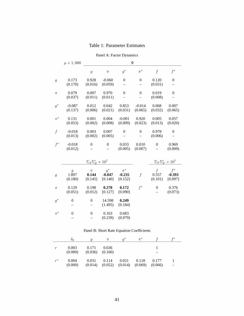
Table 1: Parameter Estimates

Panel A: Factor Dynamics

µ× 1, 000 Φ

g π g∗ π∗ f f∗

g 0.173 0.928 -0.060 0 0 0.120 0(0.170) (0.016) (0.059) – – (0.031) –

π 0.079 0.007 0.970 0 0 0.019 0(0.037) (0.011) (0.011) – – (0.008) –

g∗ -0.087 0.012 0.042 0.853 -0.014 0.068 0.007(0.137) (0.006) (0.021) (0.031) (0.065) (0.032) (0.065)

π∗ 0.131 0.001 0.004 -0.001 0.920 0.005 0.057(0.053) (0.002) (0.008) (0.009) (0.023) (0.013) (0.020)

f -0.018 0.003 0.007 0 0 0.978 0(0.013) (0.002) (0.005) – – (0.006) –

f∗ -0.018 0 0 0.033 0.010 0 0.969(0.012) – – (0.005) (0.007) – (0.009)

ΣZΣ′Z × 107 ΣF Σ′F × 107

g π g∗ π∗ f f∗g 1.897 0.144 -0.047 -0.235 f 0.557 -0.393

(0.180) [0.145] [0.140] [0.152] (0.101) [0.097]

π 0.129 0.198 0.278 0.172 f∗ 0 0.376(0.051) (0.012) [0.127] [0.090] – (0.073)

g∗ 0 0 14.598 0.249– – (1.495) [0.184]

π∗ 0 0 0.163 0.683– – (0.239) (0.079)

Panel B: Short Rate Equation Coefficients

δ0 g π g∗ π∗ f f∗

r 0.003 0.171 0.636 1(0.000) (0.036) (0.160) –

r∗ 0.004 0.031 0.114 0.021 0.118 0.177 1(0.000) (0.014) (0.052) (0.014) (0.069) (0.066) –

41

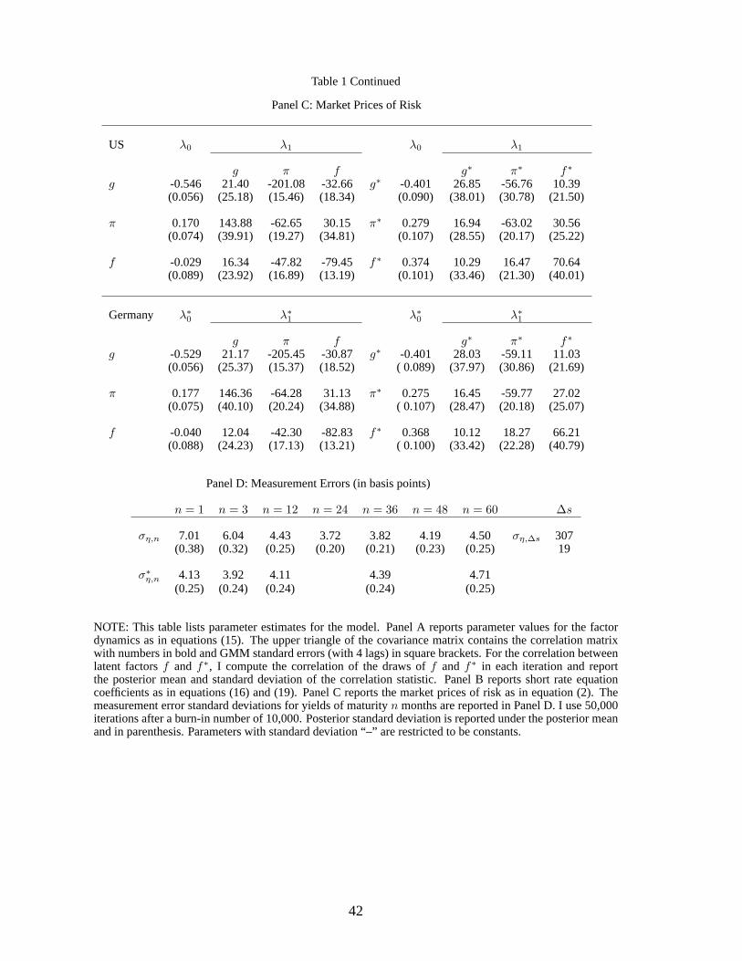
Table 1 Continued

Panel C: Market Prices of Risk

US λ0 λ1 λ0 λ1

g π f g∗ π∗ f∗g -0.546 21.40 -201.08 -32.66 g∗ -0.401 26.85 -56.76 10.39

(0.056) (25.18) (15.46) (18.34) (0.090) (38.01) (30.78) (21.50)

π 0.170 143.88 -62.65 30.15 π∗ 0.279 16.94 -63.02 30.56(0.074) (39.91) (19.27) (34.81) (0.107) (28.55) (20.17) (25.22)

f -0.029 16.34 -47.82 -79.45 f∗ 0.374 10.29 16.47 70.64(0.089) (23.92) (16.89) (13.19) (0.101) (33.46) (21.30) (40.01)

Germany λ∗0 λ∗1 λ∗0 λ∗1

g π f g∗ π∗ f∗g -0.529 21.17 -205.45 -30.87 g∗ -0.401 28.03 -59.11 11.03

(0.056) (25.37) (15.37) (18.52) ( 0.089) (37.97) (30.86) (21.69)

π 0.177 146.36 -64.28 31.13 π∗ 0.275 16.45 -59.77 27.02(0.075) (40.10) (20.24) (34.88) ( 0.107) (28.47) (20.18) (25.07)

f -0.040 12.04 -42.30 -82.83 f∗ 0.368 10.12 18.27 66.21(0.088) (24.23) (17.13) (13.21) ( 0.100) (33.42) (22.28) (40.79)

Panel D: Measurement Errors (in basis points)

n = 1 n = 3 n = 12 n = 24 n = 36 n = 48 n = 60 ∆s

ση,n 7.01 6.04 4.43 3.72 3.82 4.19 4.50 ση,∆s 307(0.38) (0.32) (0.25) (0.20) (0.21) (0.23) (0.25) 19

σ∗η,n 4.13 3.92 4.11 4.39 4.71(0.25) (0.24) (0.24) (0.24) (0.25)

NOTE: This table lists parameter estimates for the model. Panel A reports parameter values for the factordynamics as in equations (15). The upper triangle of the covariance matrix contains the correlation matrixwith numbers in bold and GMM standard errors (with 4 lags) in square brackets. For the correlation betweenlatent factorsf and f∗, I compute the correlation of the draws off and f∗ in each iteration and reportthe posterior mean and standard deviation of the correlation statistic. Panel B reports short rate equationcoefficients as in equations (16) and (19). Panel C reports the market prices of risk as in equation (2). Themeasurement error standard deviations for yields of maturityn months are reported in Panel D. I use 50,000iterations after a burn-in number of 10,000. Posterior standard deviation is reported under the posterior meanand in parenthesis. Parameters with standard deviation “–” are restricted to be constants.

42

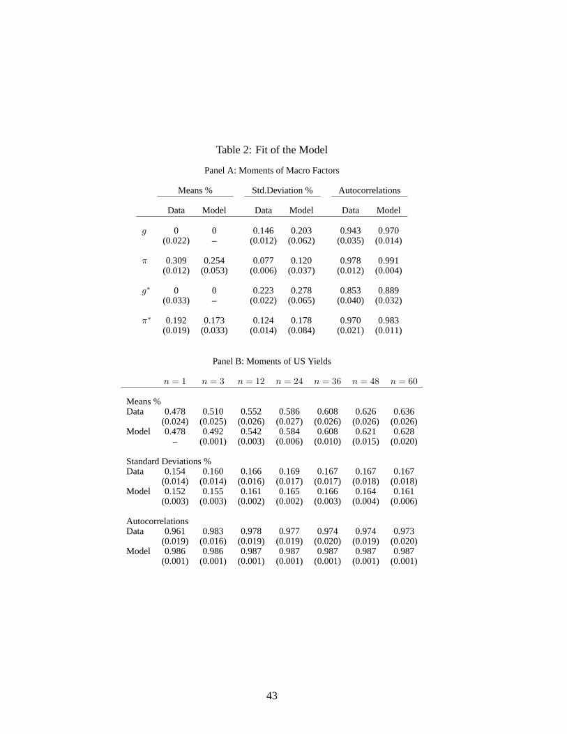
Table 2: Fit of the Model

Panel A: Moments of Macro Factors

Means % Std.Deviation % Autocorrelations

Data Model Data Model Data Model

g 0 0 0.146 0.203 0.943 0.970(0.022) – (0.012) (0.062) (0.035) (0.014)

π 0.309 0.254 0.077 0.120 0.978 0.991(0.012) (0.053) (0.006) (0.037) (0.012) (0.004)

g∗ 0 0 0.223 0.278 0.853 0.889(0.033) – (0.022) (0.065) (0.040) (0.032)

π∗ 0.192 0.173 0.124 0.178 0.970 0.983(0.019) (0.033) (0.014) (0.084) (0.021) (0.011)

Panel B: Moments of US Yields

n = 1 n = 3 n = 12 n = 24 n = 36 n = 48 n = 60

Means %Data 0.478 0.510 0.552 0.586 0.608 0.626 0.636

(0.024) (0.025) (0.026) (0.027) (0.026) (0.026) (0.026)Model 0.478 0.492 0.542 0.584 0.608 0.621 0.628

– (0.001) (0.003) (0.006) (0.010) (0.015) (0.020)

Standard Deviations %Data 0.154 0.160 0.166 0.169 0.167 0.167 0.167

(0.014) (0.014) (0.016) (0.017) (0.017) (0.018) (0.018)Model 0.152 0.155 0.161 0.165 0.166 0.164 0.161

(0.003) (0.003) (0.002) (0.002) (0.003) (0.004) (0.006)

AutocorrelationsData 0.961 0.983 0.978 0.977 0.974 0.974 0.973

(0.019) (0.016) (0.019) (0.019) (0.020) (0.019) (0.020)Model 0.986 0.986 0.987 0.987 0.987 0.987 0.987

(0.001) (0.001) (0.001) (0.001) (0.001) (0.001) (0.001)

43

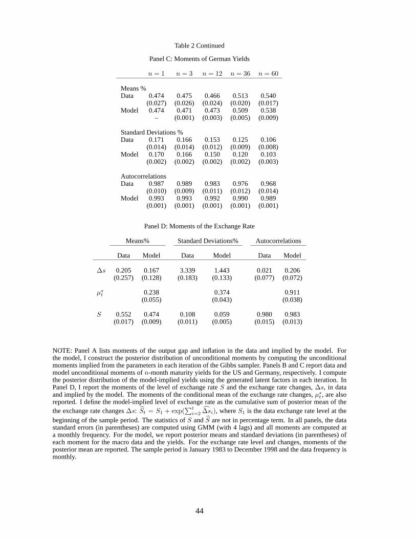
Table 2 Continued

Panel C: Moments of German Yields

n = 1 n = 3 n = 12 n = 36 n = 60

Means %Data 0.474 0.475 0.466 0.513 0.540

(0.027) (0.026) (0.024) (0.020) (0.017)Model 0.474 0.471 0.473 0.509 0.538

– (0.001) (0.003) (0.005) (0.009)

Standard Deviations %Data 0.171 0.166 0.153 0.125 0.106

(0.014) (0.014) (0.012) (0.009) (0.008)Model 0.170 0.166 0.150 0.120 0.103

(0.002) (0.002) (0.002) (0.002) (0.003)

AutocorrelationsData 0.987 0.989 0.983 0.976 0.968

(0.010) (0.009) (0.011) (0.012) (0.014)Model 0.993 0.993 0.992 0.990 0.989

(0.001) (0.001) (0.001) (0.001) (0.001)

Panel D: Moments of the Exchange Rate

Means% Standard Deviations% Autocorrelations

Data Model Data Model Data Model

∆s 0.205 0.167 3.339 1.443 0.021 0.206(0.257) (0.128) (0.183) (0.133) (0.077) (0.072)

µst 0.238 0.374 0.911

(0.055) (0.043) (0.038)

S 0.552 0.474 0.108 0.059 0.980 0.983(0.017) (0.009) (0.011) (0.005) (0.015) (0.013)

NOTE: Panel A lists moments of the output gap and inflation in the data and implied by the model. Forthe model, I construct the posterior distribution of unconditional moments by computing the unconditionalmoments implied from the parameters in each iteration of the Gibbs sampler. Panels B and C report data andmodel unconditional moments ofn-month maturity yields for the US and Germany, respectively. I computethe posterior distribution of the model-implied yields using the generated latent factors in each iteration. InPanel D, I report the moments of the level of exchange rateS and the exchange rate changes,∆s, in dataand implied by the model. The moments of the conditional mean of the exchange rate changes,µs

t , are alsoreported. I define the model-implied level of exchange rate as the cumulative sum of posterior mean of thethe exchange rate changes∆s: St = S1 + exp(

∑ti=2 ∆si), whereS1 is the data exchange rate level at the

beginning of the sample period. The statistics ofS andS are not in percentage term. In all panels, the datastandard errors (in parentheses) are computed using GMM (with 4 lags) and all moments are computed ata monthly frequency. For the model, we report posterior means and standard deviations (in parentheses) ofeach moment for the macro data and the yields. For the exchange rate level and changes, moments of theposterior mean are reported. The sample period is January 1983 to December 1998 and the data frequency ismonthly.

44

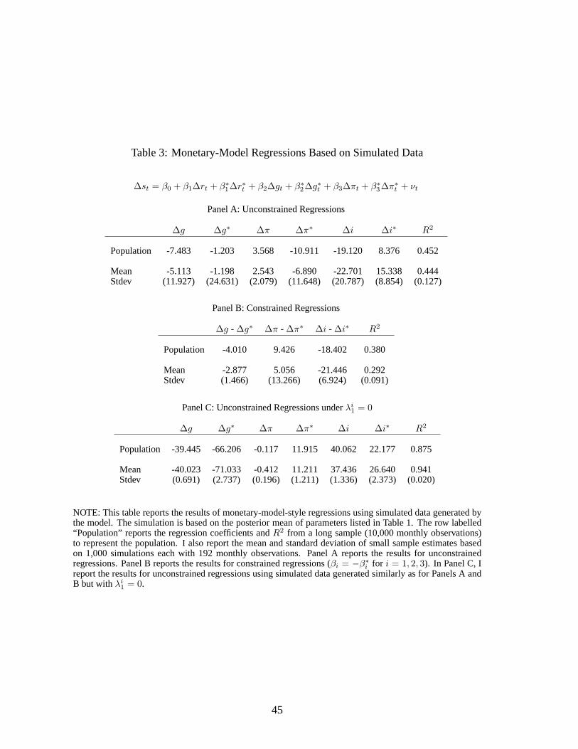
Table 3: Monetary-Model Regressions Based on Simulated Data

∆st = β0 + β1∆rt + β∗1∆r∗t + β2∆gt + β∗2∆g∗t + β3∆πt + β∗3∆π∗t + νt

Panel A: Unconstrained Regressions

∆g ∆g∗ ∆π ∆π∗ ∆i ∆i∗ R2

Population -7.483 -1.203 3.568 -10.911 -19.120 8.376 0.452

Mean -5.113 -1.198 2.543 -6.890 -22.701 15.338 0.444Stdev (11.927) (24.631) (2.079) (11.648) (20.787) (8.854) (0.127)

Panel B: Constrained Regressions

∆g - ∆g∗ ∆π - ∆π∗ ∆i - ∆i∗ R2

Population -4.010 9.426 -18.402 0.380

Mean -2.877 5.056 -21.446 0.292Stdev (1.466) (13.266) (6.924) (0.091)

Panel C: Unconstrained Regressions underλi1 = 0

∆g ∆g∗ ∆π ∆π∗ ∆i ∆i∗ R2

Population -39.445 -66.206 -0.117 11.915 40.062 22.177 0.875

Mean -40.023 -71.033 -0.412 11.211 37.436 26.640 0.941Stdev (0.691) (2.737) (0.196) (1.211) (1.336) (2.373) (0.020)

NOTE: This table reports the results of monetary-model-style regressions using simulated data generated bythe model. The simulation is based on the posterior mean of parameters listed in Table 1. The row labelled“Population” reports the regression coefficients andR2 from a long sample (10,000 monthly observations)to represent the population. I also report the mean and standard deviation of small sample estimates basedon 1,000 simulations each with 192 monthly observations. Panel A reports the results for unconstrainedregressions. Panel B reports the results for constrained regressions (βi = −β∗i for i = 1, 2, 3). In Panel C, Ireport the results for unconstrained regressions using simulated data generated similarly as for Panels A andB but withλi

1 = 0.

45

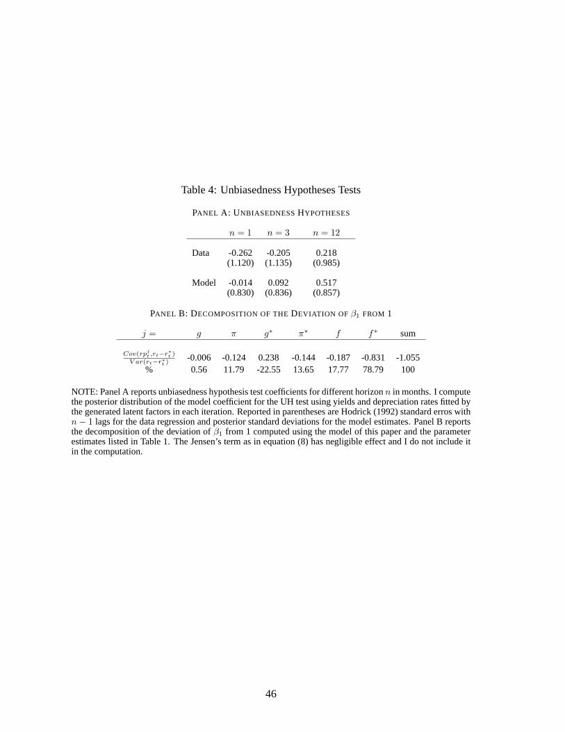
Table 4: Unbiasedness Hypotheses Tests

PANEL A: UNBIASEDNESSHYPOTHESES

n = 1 n = 3 n = 12

Data -0.262 -0.205 0.218(1.120) (1.135) (0.985)

Model -0.014 0.092 0.517(0.830) (0.836) (0.857)

PANEL B: DECOMPOSITION OF THEDEVIATION OF β1 FROM 1

j = g π g∗ π∗ f f∗ sum

Cov(rpjt ,rt−r∗t )

V ar(rt−r∗t ) -0.006 -0.124 0.238 -0.144 -0.187 -0.831 -1.055% 0.56 11.79 -22.55 13.65 17.77 78.79 100

NOTE: Panel A reports unbiasedness hypothesis test coefficients for different horizonn in months. I computethe posterior distribution of the model coefficient for the UH test using yields and depreciation rates fitted bythe generated latent factors in each iteration. Reported in parentheses are Hodrick (1992) standard erros withn− 1 lags for the data regression and posterior standard deviations for the model estimates. Panel B reportsthe decomposition of the deviation ofβ1 from 1 computed using the model of this paper and the parameterestimates listed in Table 1. The Jensen’s term as in equation (8) has negligible effect and I do not include itin the computation.

46

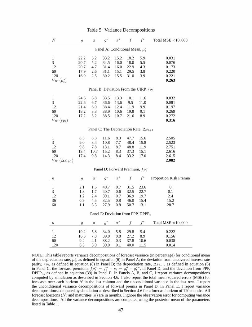
Table 5: Variance Decompositions

N g π g∗ π∗ f f∗ Total MSE×10, 000

Panel A: Conditional Mean,µst

1 22.2 5.2 33.2 15.2 18.2 5.9 0.0313 20.7 5.2 34.5 16.0 18.0 5.5 0.07612 20.7 4.7 31.4 16.0 22.9 4.3 0.17360 17.9 2.6 31.1 15.1 29.5 3.8 0.220120 16.9 2.5 30.2 15.5 31.0 3.9 0.221V ar(µs

t ) 0.263

Panel B: Deviation From the UIRP,rpt

1 24.6 6.8 33.5 13.3 10.1 11.6 0.0323 22.6 6.7 36.6 13.6 9.5 11.0 0.08112 21.4 6.0 38.4 12.4 11.9 9.9 0.19760 18.2 3.3 38.9 10.6 19.8 9.1 0.269120 17.2 3.2 38.5 10.7 21.6 8.9 0.272V ar(rpt) 0.316

Panel C: The Depreciation Rate,∆st+1

1 8.5 8.3 11.6 8.3 47.7 15.6 2.5053 9.0 8.4 10.8 7.7 48.4 15.8 2.52312 9.8 7.8 13.1 8.7 48.8 11.9 2.75160 13.4 10.7 15.2 8.3 37.3 15.1 2.616120 17.4 9.8 14.3 8.4 33.2 17.0 2.615V ar(∆st+1) 2.082

Panel D: Forward Premium,fpnt

n g π g∗ π∗ f f∗ Proportion Risk Premia

1 2.1 1.5 40.7 0.7 31.5 23.6 03 1.8 1.7 40.7 0.6 32.5 22.7 0.112 1.2 2.4 39.1 0.7 36.9 19.7 2.436 0.9 4.5 32.5 0.8 46.0 15.4 15.260 1.1 6.5 27.9 0.8 50.7 13.1 28.7

Panel E: Deviation from PPP, DPPPn

n g π g∗ π∗ f f∗ Total MSE×10, 000

1 19.2 5.8 34.0 5.8 29.8 5.4 0.22212 16.3 7.8 39.0 0.8 27.2 8.9 0.15660 9.2 4.1 38.2 0.3 37.8 10.6 0.038120 6.3 3.0 39.0 0.1 40.0 11.5 0.014

NOTE: This table reports variance decompositions of forecast variance (in percentage) for conditional meanof the depreciation rate,µs

t , as defined in equation (6) in Panel A; the deviation from uncovered interest rateparity, rpt, as defined in equation (8) in Panel B; the depreciation rate,∆st+1, as defined in equation (6)in Panel C; the forward premium,fpn

t = fnt − st = yn

t − y∗nt , in Panel D; and the deviation from PPP,DPPPn, as defined in equation (39) in Panel E. In Panels A, B, and C, I report variance decompositionscomputed by simulation as described in Section 4.6. I also report the total mean squared errors (MSE) forforecasts over each horizonN in the last column and the unconditional variance in the last row. I reportthe unconditional variance decompositions of forward premia in Panel D. In Panel E, I report variancedecompositions computed by simulation as described in Section 4.6 for a forecast horizon of120 months. Allforecast horizons (N ) and maturities (n) are in months. I ignore the observation error for computing variancedecompositions. All the variance decompositions are computed using the posterior mean of the parameterslisted in Table 1.

47

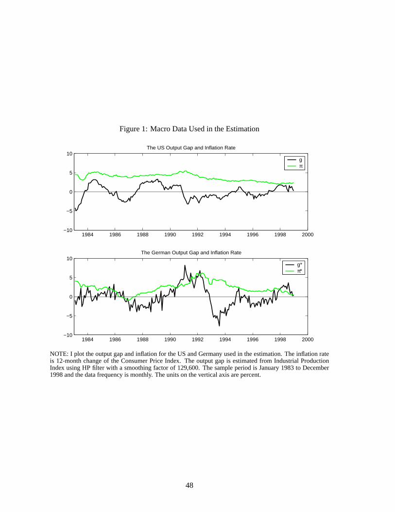
Figure 1: Macro Data Used in the Estimation

1984 1986 1988 1990 1992 1994 1996 1998 2000−10

−5

0

5

10The US Output Gap and Inflation Rate

gπ

1984 1986 1988 1990 1992 1994 1996 1998 2000−10

−5

0

5

10The German Output Gap and Inflation Rate

g*π*

NOTE: I plot the output gap and inflation for the US and Germany used in the estimation. The inflation rateis 12-month change of the Consumer Price Index. The output gap is estimated from Industrial ProductionIndex using HP filter with a smoothing factor of 129,600. The sample period is January 1983 to December1998 and the data frequency is monthly. The units on the vertical axis are percent.

48

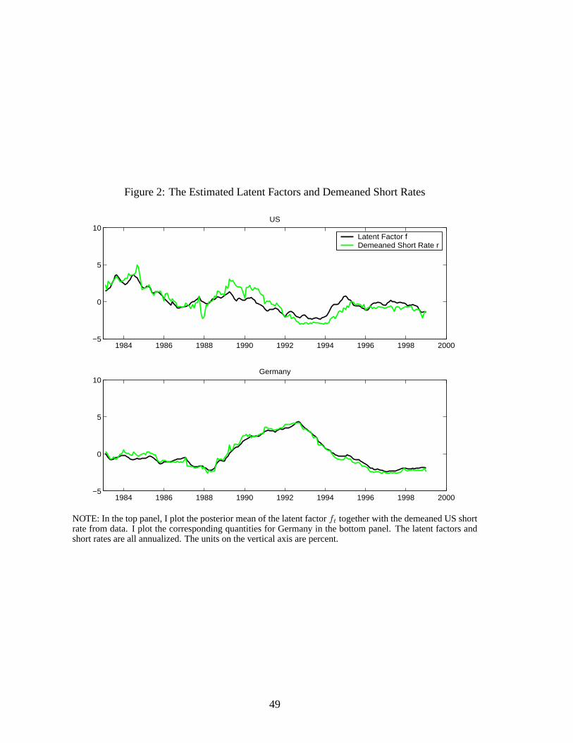
Figure 2: The Estimated Latent Factors and Demeaned Short Rates

1984 1986 1988 1990 1992 1994 1996 1998 2000−5

0

5

10 US

Latent Factor fDemeaned Short Rate r

1984 1986 1988 1990 1992 1994 1996 1998 2000−5

0

5

10 Germany

NOTE: In the top panel, I plot the posterior mean of the latent factorft together with the demeaned US shortrate from data. I plot the corresponding quantities for Germany in the bottom panel. The latent factors andshort rates are all annualized. The units on the vertical axis are percent.

49

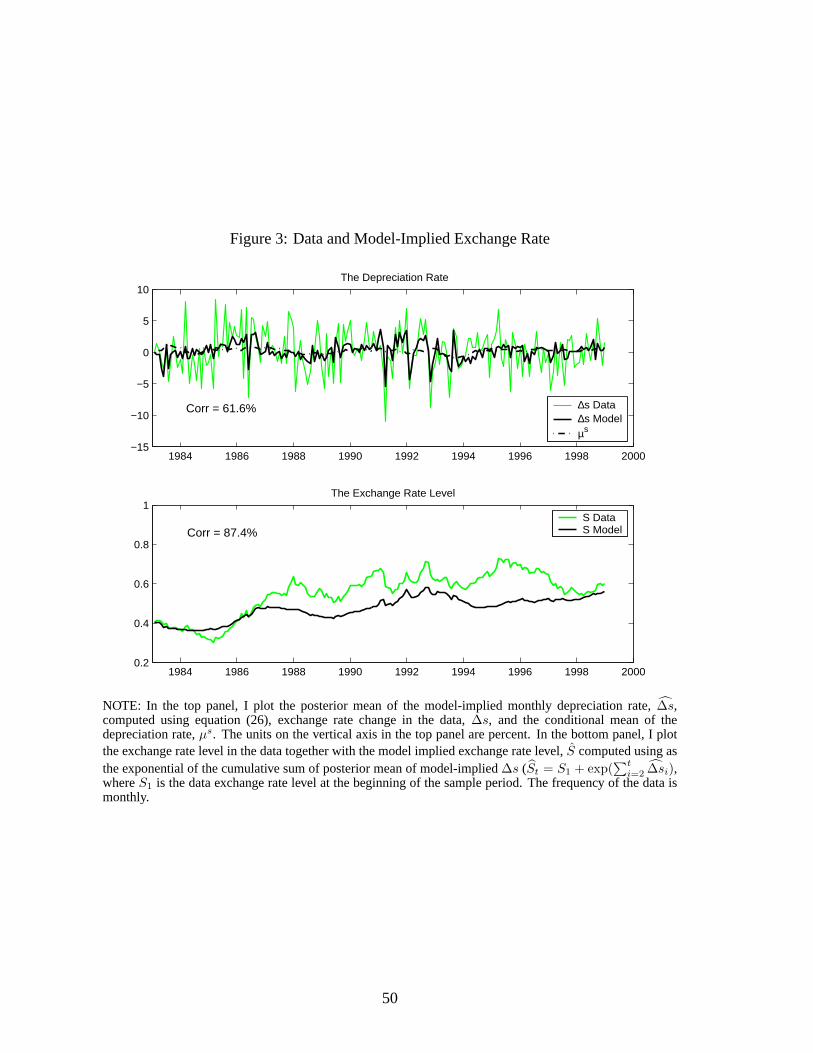
Figure 3: Data and Model-Implied Exchange Rate

1984 1986 1988 1990 1992 1994 1996 1998 2000−15

−10

−5

0

5

10 The Depreciation Rate

∆s Data∆s Modelµs

1984 1986 1988 1990 1992 1994 1996 1998 20000.2

0.4

0.6

0.8

1The Exchange Rate Level

S DataS Model

Corr = 61.6%

Corr = 87.4%

NOTE: In the top panel, I plot the posterior mean of the model-implied monthly depreciation rate,∆s,computed using equation (26), exchange rate change in the data,∆s, and the conditional mean of thedepreciation rate,µs. The units on the vertical axis in the top panel are percent. In the bottom panel, I plotthe exchange rate level in the data together with the model implied exchange rate level,S computed using asthe exponential of the cumulative sum of posterior mean of model-implied∆s (St = S1 + exp(

∑ti=2 ∆si),

whereS1 is the data exchange rate level at the beginning of the sample period. The frequency of the data ismonthly.

50

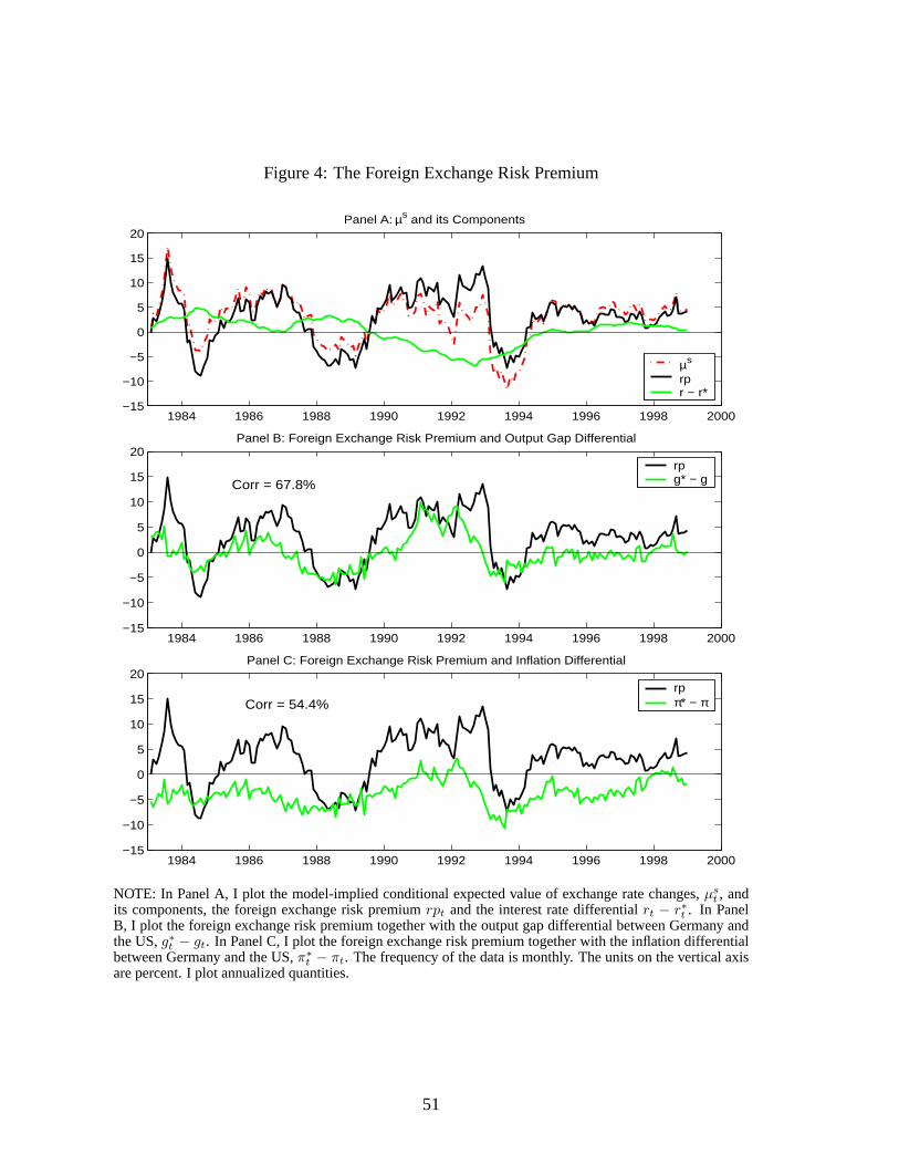
Figure 4: The Foreign Exchange Risk Premium

1984 1986 1988 1990 1992 1994 1996 1998 2000−15

−10

−5

0

5

10

15

20Panel A: µs and its Components

µs

rpr − r*

1984 1986 1988 1990 1992 1994 1996 1998 2000−15

−10

−5

0

5

10

15

20Panel B: Foreign Exchange Risk Premium and Output Gap Differential

rpg* − gCorr = 67.8%

1984 1986 1988 1990 1992 1994 1996 1998 2000−15

−10

−5

0

5

10

15

20Panel C: Foreign Exchange Risk Premium and Inflation Differential

rpπ* − πCorr = 54.4%

NOTE: In Panel A, I plot the model-implied conditional expected value of exchange rate changes,µst , and

its components, the foreign exchange risk premiumrpt and the interest rate differentialrt − r∗t . In PanelB, I plot the foreign exchange risk premium together with the output gap differential between Germany andthe US,g∗t − gt. In Panel C, I plot the foreign exchange risk premium together with the inflation differentialbetween Germany and the US,π∗t − πt. The frequency of the data is monthly. The units on the vertical axisare percent. I plot annualized quantities.

51

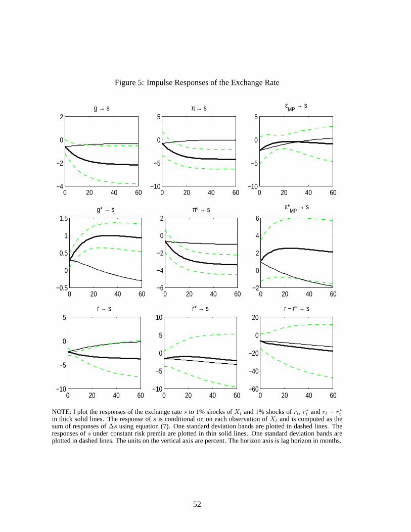
Figure 5: Impulse Responses of the Exchange Rate

0 20 40 60−4

−2

0

2g → s

0 20 40 60−10

−5

0

5π → s

0 20 40 60−10

−5

0

5

εMP

→ s

0 20 40 60−0.5

0

0.5

1

1.5g* → s

0 20 40 60−6

−4

−2

0

2π* → s

0 20 40 60−2

0

2

4

6

ε*MP

→ s

0 20 40 60−60

−40

−20

0

20r − r* → s

0 20 40 60−10

−5

0

5r → s

0 20 40 60−10

−5

0

5

10r* → s

NOTE: I plot the responses of the exchange rates to 1% shocks ofXt and 1% shocks ofrt, r∗t andrt − r∗tin thick solid lines. The response ofs is conditional on on each observation ofXt and is computed as thesum of responses of∆s using equation (7). One standard deviation bands are plotted in dashed lines. Theresponses ofs under constant risk premia are plotted in thin solid lines. One standard deviation bands areplotted in dashed lines. The units on the vertical axis are percent. The horizon axis is lag horizon in months.

52

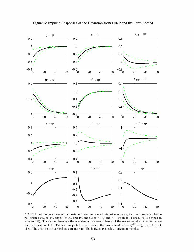
Figure 6: Impulse Responses of the Deviation from UIRP and the Term Spread

0 20 40 60−0.3

−0.2

−0.1

0

0.1g → rp

0 20 40 60−0.6

−0.4

−0.2

0

0.2π → rp

0 20 40 60−0.2

0

0.2

0.4

0.6

εMP

→ rp

0 20 40 600

0.1

0.2

0.3

0.4

ε*MP

→ rp

0 20 40 600

0.05

0.1g* → rp

0 20 40 60−0.3

−0.2

−0.1

0

0.1π* → rp

0 20 40 60−2

−1

0

1r − r* → rp

0 20 40 60−0.4

−0.2

0

0.2

0.4r* → rp

0 20 40 60−0.4

−0.2

0

0.2

0.4r → rp

0 20 40 60−0.1

0

0.1

0.2

0.3r → sp*

0 20 40 60−0.2

−0.1

0

0.1r → sp

0 20 40 60

−0.4

−0.3

−0.2

−0.1

0

0.1r* → sp*

NOTE: I plot the responses of the deviation from uncovered interest rate parity, i.e., the foreign exchangerisk premiarpt, to 1% shocks ofXt and 1% shocks ofrt, r∗t andrt − r∗t in solid lines. rp is defined inequation (8). The dashed lines are the one standard deviation bands of the responses ofrp conditional oneach observation ofXt. The last row plots the responses of the term spread,spi

t = yi,60t − ri

t, to a 1% shockof ri

t. The units on the vertical axis are percent. The horizon axis is lag horizon in months.

53

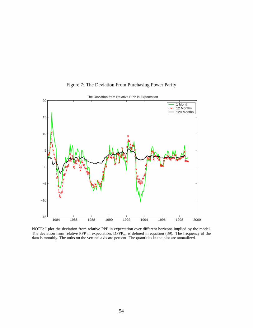
Figure 7: The Deviation From Purchasing Power Parity

1984 1986 1988 1990 1992 1994 1996 1998 2000−15

−10

−5

0

5

10

15

20The Deviation from Relative PPP in Expectation

1 Month12 Months120 Months

NOTE: I plot the deviation from relative PPP in expectation over different horizons implied by the model.The deviation from relative PPP in expectation, DPPPn, is defined in equation (39). The frequency of thedata is monthly. The units on the vertical axis are percent. The quantities in the plot are annualized.

54